Influence of Speed Limit on Roadway Safety in Indiana

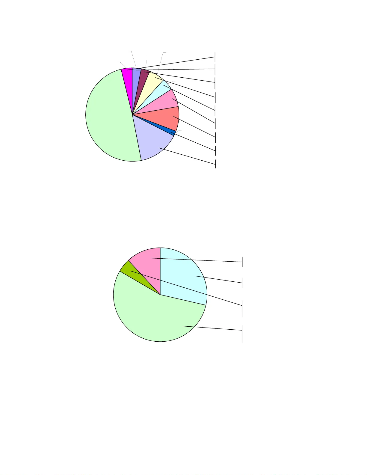
INFLUENCE OF SPEED LIMIT ON ROADWAY SAFETY IN INDIANA A Thesis Submitted to the Faculty of Purdue University by Nataliya V. Malyshkina In Partial Fulfillment of the Requirements fo r the Degree of Master of Science in Civil Engineering December 2006 Purdue University West Lafayette, Indiana ii To my mother, father and husband iii ACKNOWLEDGMENTS I would first like to thank my advisor, Professor Fred Mannering. Without his expert advice and his support none of this research would be possible. Not only has he always helped and gu ided me, but he also carefully listened t o my opinions and suggestions on the research. I am lucky to be his student. I would like to thank Professor Kristo fer Jennings and especially Professor Andrew Tarko for their very helpful comments and for carefully reading the thesis. I would also like to thank Doro thy Miller, Maeve Drummond and Marcie Duffin for their help in completing all administrative procedures and requirements for the M. S. thesis defense. I am deeply indebted to my colleagues at t he Ural State University of Railroad Transportation in Russia, where I obtained my first research and teaching experience. This thesis and my graduate studies at Purdue University would never be possible without their s upport and encouragement years ago. Finally, I feel endless grat itude and love to my wonder ful family – my mother, Nadezhda, my father, Vladimir, and my husband, Leonid. I owe everything I have to them and to thei r love and support. iv TABLE OF CONTENTS Page ACKNOWLEDGMENTS iii TABLE OF CONTENTS iv LIST OF TABLES v LIST OF FIGURES vi ABSTRACT vii CHAPTER 1. INTRODUCTION 1 CHAPTER 2. METHODOLOGY OF STATISTICAL MODELING 10 CHAPTER 3. DATA DESCRIPTION 17 3.1. Accident data for year 2004 ................................................................... 18 3.2. Accident data for year 2006 ................................................................... 23 CHAPTER 4. ACCIDENT CAUSATION STUDY 27 4.1. Modeling Procedures: accident c ausatio n .............................................. 27 4.2. Results: accident causation models ....................................................... 34 4.2.1. Effect of Speed Li mit ........................................................................ 35 4.2.2. Effect of Other Explanatory Va riables .............................................. 40 CHAPTER 5. ACCIDENT SEVERITY STUDY 42 5.1. Modeling Procedures: accident se verity ................................................. 42 5.2. Results: accident severity models .......................................................... 44 5.2.1. Effect of Speed Li mit ........................................................................ 45 5.2.2. Effect of Other Explanatory Va riables .............................................. 50 CHAPTER 6. DISCUSSION 54 LIST OF REFERENCES 59 Appendix A. ................................................................................................... 62 Appendix B. ................................................................................................... 65 Appendix C. ................................................................................................... 92 v LIST OF TABLES T a b l e P a g e Table 4.1 2004 accident causation models: results for speed limit ................... 36 Table 4.2 2006 accident causation models: results for speed limit ................... 37 Table 5.1 2004 accident severity models: results for speed limit ...................... 46 Table 5.2 2006 accident severity models: results for speed limit ...................... 47 Table 5.3 Speed limit effect on structure of 2004 acci dent severity models ...... 48 Table 5.4 Speed limit effect on structure of 2006 acci dent severity models ...... 49 Table B.1 Road classes & accident types in 2004 accident causation study .... 65 Table B.2 Road classes & accident types in 2006 accident causation study .... 66 Table B.3 Binary logit models fo r 2004 accident causatio n ............................... 67 Table B.4 Binary logit models fo r 2006 accident causatio n ............................... 78 Table B.5 Tests of car-SUV separation in 2004 accident causation study ........ 90 Table B.6 Tests of car-SUV separation in 2006 accident causation study ........ 91 Table C.1 Road classes and accident types in 2004 accident severity study.... 92 Table C.2 Road classes and accident types in 2006 accident severity study.... 93 Table C.3 Speed limit data bins chosen in 2004 accident severity study .......... 94 Table C.4 Speed limit data bins chosen in 2006 accident severity study .......... 95 Table C.5 Multinomial logit m odels for 2004 accident severity .......................... 96 Table C.6 Multinomial logit m odels for 2006 accident severity ........................ 126 Table C.7 Tests of car-SUV separation in 2004 accident severity study ......... 153 Table C.8 Tests of car-SUV separation in 2006 accident severity study ......... 154 vi LIST OF FIGURES Figure Page Figure 3.1 Percentage distribution of 2004 accidents by road class ................. 19 Figure 3.2 Percentage distribution of 2004 accidents by their type ................... 19 Figure 3.3 Percentage distribution of 2004 accidents by their causation .......... 20 Figure 3.4 Percentage distribution of 2004 accidents by their severity level ..... 21 Figure 3.5 Percentage distributions of 2004 accidents by their causation in four different speed limit data bins ...................................................................... 21 Figure 3.6 Percentage distributions of 2004 accidents by their severity level in four different speed limit data bins .............................................................. 22 Figure 3.7 Percentage distribution of 2006 accidents by road class ................. 23 Figure 3.8 Percentage distribution of 2006 accidents by their type ................... 24 Figure 3.9 Percentage distribution of 2006 accidents by their causation .......... 24 Figure 3.10 Percentage distri bution of 2006 accidents by their severity level ... 25 Figure 3.11 Percentage distri butions of 2006 accidents by their causation in four different speed limit data bins ...................................................................... 25 Figure 3.12 Percentage distri butions of 2006 accidents by their severity level in four different speed limit data bins .............................................................. 26 Figure 4.1 Data division by r oad class and by a ccident ty pe ............................. 29 Figure 4.2 Model esti mation proc edures ........................................................... 31 Figure 4.3 T-ratios of statistically si gnificant speed limit coefficients in 2004 accident causat ion model s .......................................................................... 39 Figure 4.4 T-ratios of statistically si gnificant speed limit coefficients in 2006 accident causat ion model s .......................................................................... 39 vii ABSTRACT Malyshkina, Nataliya V. M.S., Purdue University, December 2006. Influence of Speed Limit on Roadway Safety in Indiana. Major Professor: Fred Mannering. The influence of speed limits on roadway sa fety is an extremel y important social issue and is subject to an extensive debate in the State of Indiana and nationwide. With around 800- 900 fatalities and thousands of injuries annually in Indiana, traffic accidents place an incredi ble social and economic burden on the state. Still, speed limits posted on highways and ot her roads are routinely exceeded as individual driv ers try to balance safety and mobility (speed). This research explores the relationship between speed limits and roadway safety. Namely, the research focuses on the in fluence of the posted speed limit on the causation and severity of accidents. Da ta on individual accidents from the Indiana Electronic Vehicle Crash Record System is used in the research, and appropriate statistical models are estima ted for causation and severity of different types of accidents on all road classes. The results of the modeling show that speed limits do not have a statis tically significant adverse effect on unsafe-speed-related causati on of accidents on all roads, but generally increase the severity of accidents on the majori ty of roads other than highways (the accident severity on highways is unaffected by speed limits). Our findings can perhaps save both lives and travel time by helping the Indiana Department of Transportation determine optimal speed limit policies in the state. 1 CHAPTER 1. INTRODUCTION A new law, which took effect on July 1, 2005, made Indiana the 30 th U.S. state to raise interstate speed limits up to 70 mph. The top s peed limit value was increased on some portions of the stat e’s interstate highway system from 65 mph to 70 mph. This increas e intensified an important debate in the engineering community on the tradeoff between highwa y mobility (speed) and safety. On one hand, as speed increases, travel times decrease, which reduces transportation costs and leads to an incr eased productivity and a noticeable positive effect for the nat ional economy. On the ot her hand, higher speed can possibly have a negative effect on roadway safety. The relationship between speed limits and roadw ay safety is not as obvious as it seems. The reason is that there are several important i ssues in this relationship. On one hand, as speed increases, vehicles have higher kinetic energy, travel larger distances during hum an reaction times, and vehicles are exposed to stronger aerodynamic and centrifugal. This tends to increase accident frequency and severity. On the other hand, as speed increases, the variance of vehic le velocities may decrease, resulting in easier and safer driving conditions. As a result, the overall effect of a speed limit increase on road safety is complic ated, and requires a thorough study. Such a study and a detailed analysis of the relationship between speed limits and safety on Indiana roads will be undertaken in this thesis. In general, there are two measures of road safety that are commonly considered: 2 1. The first measure evaluates acci dent frequencies on roadway s ections. The accident frequency on a road section is obtained by counting the number of accidents occurring on this se ction during a specified period of time. Then count-data statistical models (e.g. Poisson, negative binomial models and their zero-inflated counter parts) are estimated for accident frequencies on different road sections. The explanatory variables used in these models are the road section characteristics (e.g. road section length, curvature, slope, type, etc). 2. The second measure evaluates accident severity outcomes as determined by the injury level sustained by the most severely injured individual (if any) involved into the a ccident. This evaluation is done by using data on individual accidents and estimating discrete outcome statistical models (e.g. ordered probit and multinomial logit models) for the accident severity outcomes. The explanatory variables used in these models are the individual accident characteristics (e.g. time and location of an accident, weather conditions and road characteristics at the accident location, characteristics of the vehicles and drivers involved, etc). These two measures of read safety are complementary. On one hand, an accident frequency study gives a statisti cal model of the probability of an accident occurring on a road section. On the other hand, an accident severity study gives a statistical model of the conditional probabilit y of a severity outcome of an accident, given an a ccident occurred. The unconditional probability of the acci dent severity outcome is the product of its conditional probability and the accident probability. The number of road safety studies that consider one or both of the two road safety measures described above is enorm ous. Some of the key studies include the following: 3 • Shankar et al. (1996) used a nested l ogit model for statistical analysis of accident severity outcomes on rural hi ghways in Washington State. They found that environment conditions, highw ay design, accident type, driver and vehicle characteristics significantly influence accident severity. They found that overturn accidents, r ear-end accidents on wet pavement, fixed-object accidents, and failures to use the restraint belt system lead to higher probabilities of inju ry or/and fatality accident outcomes, while icy pavement and single-vehicle collisions lead to higher probability of property damage only outcomes. • Shankar et al. (1997) studied the distinction between safe and unsafe road sections by estimating zero-i nflated Poisson and zero-inflated negative binomial models for accident frequencies in Washington State (for these models the zero state corresponds to near zero accident likelihood on safe road sections). • Duncan et al. (1998) applied an ordered probit model to injury severity outcomes in truck-passenger car rear-e nd collisions in North Carolina. They found that injury severity is increased by darkness, high speed differentials, high speed limits, wet grades, drunk driving, and being female. • Karlaftis and Tarko (1998) considered heterogeneous panel data for frequencies of accidents occurred in Indi ana over a 6-year period. They developed an improved me thod of accident frequen cy modeling in panel data, which is based on a two-step approach: first, heterogeneous data is divided into homogeneous groups by determining (dis)similarities and using cluster analysis; second, negative binomial models are estimated separately for each homogeneous data group. The results obtained by Karlaftis and Tarko clearly indicate t hat there are significant differences between the accident frequency models estimated for urban, suburban and rural counties. 4 • Chang and Mannering (1999) focused on the effects of trucks and vehicle occupancies on accident severities. T hey estimated nested logit models for severity outcomes of truck-in volved and non-truck-involved accidents in Washington State and found that accide nt injury severity is noticeably worsened if the accident has a tru ck involved, and that the effects of trucks are more significant for multi-occupant vehicles than for single- occupant vehicles. • Carson and Mannering (2001) studied the effect of ice warning signs on ice-accident frequencies and severiti es in Washington State. They modeled accident frequencies and severi ties by using zero-inflated negative binomial and logit models re spectively. They found that the presence of ice warning signs was not a significant factor in reducing ice- accident frequencies and severities. • Khattak (2001) estimated ordered probit models for severity outcomes of multi-vehicle rear-end accidents in No rth Carolina. In particular, the results of his research indicate that in two-vehicle collisions the leading driver is more likely to be severely injured, in three-vehicle collisions the driver in the middle is more likely to be severely injur ed, and being in a newer vehicle protects the driv er in rear-end collisions. • Ulfarsson (2001) and Ulfarsson and Manne ring (2004) focused on male and female differences in analysis of accident severity. They used multinomial logit models and accident data from Washington State. They found significant behavio ral and physiological differences between genders, and also found that probability of fatal and di sabling injuries is higher for females as compared to males. • Kockelman and Kweon ( 2002) applied ordered pr obit models to modeling of driver injury severity outcomes. They used a nationwide accident data sample and found that pickups and spor t utility vehicles are les s (more) safe than passenger cars in single-vehicle (two-vehicle) collisions. 5 • Lee and Mannering (2002) estimated zero-inflated count-data models and nested logit models for frequencies and severities of run-off-roadway accidents in Washington State. They found that run-off-roadway accident frequencies can be reduced by avoidi ng cut side slopes, decreasing (increasing) the distance from outsi de shoulder edge to guardrail (light poles), and decreasing the number of isolated trees along roadway. The results of their research also show t hat run-off-roadway accident severity is increased by alcohol impaired driving, high speeds , and the presence of a guardrail. • Abdel-Aty (2003) used ordered probit models for analysis of driver injury severity outcomes at different road locations (roadway sections, signalized intersections, toll plazas) in Central Florida. He found higher probabilities of severe accident outcomes for older drivers, male drivers, those not wearing seat belt, drivers who speed, those who drive vehicles struck at the driver’s side, those w ho drive in rural areas, and drivers using electronic toll collection device (E-Pass) at toll plazas. • Kweon and Kockelman (2003) studied probabilities of accidents and accident severity outcomes for a give n fixed driver exposure (which is defined as the total miles driven). T hey used Poisson and ordered probit models, and considered a nationwi de accident data sample. After normalizing accident rates by driver exposure, the results of their study indicate that young drivers are far more crash prone than other drivers, and that sport utility vehicles and pickups are more likely to be involved in rollover accidents. • Yamamoto and Shankar (2004) appli ed biv ariate ordered probit models to an analysis of driver’s and passenger’s injury severities in collisions with fixed objects. They considered a 4-year accident data sample from Washington State and found that collis ions with leading ends of guardrail and trees tend to cause more severe in juries, while collisions with sign posts, faces of guardrail, concrete barrier or bridge and fences tend to 6 cause less severe injuries. They also found that proper use of vehicle restraint system strongly decreases t he probability of severe injuries and fatalities. • Khorashadi et al. (2005) explored t he differences of driver injury severities in rural and urban accident s involving large trucks. Using 4- years of California accident data and multinomial logit model approach, they found considerable differences between rural and urban accident injury severities. In particular, they found that the probability of severe/fatal injury increases by 26% in rural areas and by 700% in urban areas when a tractor-trailer combinat ion is involved, as opposed to a single-unit truck being involved. They also found that in accidents where alcohol or drug use is i dentified, the probability of severe/fatal injury is increased by 250% and 800% in rural and urban areas respectively. • Islam and Mannering (2006) studied driv er aging and its effect on male and female single-vehicle accident in juries in Indiana. They employed multinomial logit models and found significant differences between different genders and age groups. Specific ally, they found an increase in probabilities of fatality for young and mi ddle-aged male driv ers when they have passengers, an increase in probabilities of injury for middle-aged female drivers in vehicles 6 years ol d or older, and an increase in fatality probabilities for males older than 65 years old. • Savolainen (2006), Savolainen and M annering (2006a) and Savolainen and Mannering (2006b) focused on an important topic of motorcycle safety on Indiana roads. He used multinomial and ne sted logit models and found that poor visibility, unsafe speed, alcohol us e, not wearing a helmet, right-angle and head-on collisions, and collisions wit h fixed objects cause more severe motorcycle-involved accidents. As far, as the relationship between s peed and road safety is concerned, it has been studied in the past by considering the two measures of road safety 7 described above. Previous em pirical studies of this relationship have generally found the following two results. First, on all road classes (urban streets, highways, etc) vehicle operating speeds exceed the posted speed limit (Renski et al., 1999; Khan, 2002). Second, ther e are no sure indications that a reasonable increase in speed limit has a c onsiderable negative impact on traffic safety. For example, O ’Donnell and Connor (1996) esti mated logit and probit models for injury severity outcomes of accidents in Austra lia and determined that effects of an increase in vehicle sp eed from 42 to 100 kilometers per hour (from 26.1 mph to 62.1 mph) are surprisi ngly small. Shankar et al. (1997) used zero-inflated Poisson and zero-inflated nega tive binomial models for a study of accident frequencies. They found that a speed limit increase reduced accident frequencies on road sections in the Wester n part of Washi ngton State, and had no statistically significant effect on accident frequencies in the Eastern part. Very similar results were obtained by Milton and Ma nnering (1998), who estimated negative binomial models for frequenc ies of accidents on sections of principal arterials in Wash ington State in 1992 and 1993 and found a reduction of the frequencies with a speed limit increase. Renski et al. (1999) specifically addressed the effect of speed limit on injury severity outcomes in single-vehicle accidents on interstate highways in North Carolina . They used a pair ed- comparison analysis and ordered probit modeling. They found that while increasing speed limits from 55 to 60 m ph and from 55 to 65 mph increased the probability of sustaining mi nor and non-incapacitating in juries, increasing speed limits from 65 to 70 mph di d not have a significant effect on accident severity. A thorough analysis of speed limit policies for Indiana was recently carried out by Khan (2002). He found that while prev ious upward changes in speed limits in Indiana during the past two decades did increase spe eds observed on roads, there was no statistically significant evidenc e to indicate that such increases had a negative impact on safety. 8 In the present study we focus on t he relationship between speed and road safety. We consider data on individua l accidents and use the methodologies of statistical modeling within the framework of the accident discrete outcome analysis (refer to the second measur e of road safety discussed on page 2 above). However, our study differs from t he previous studies in that we analyze both the severity and causation of acci dents. We will compile and use data from Indiana for different types of accidents (single-vehicle accidents, car or SUV versus truck accidents, etc) on all classe s of roads (interstate highways, urban streets, US routes, etc). To analyze and understand the effect of speed limit on roadway safety, in our study we will use the following two statistical modeling approaches: 1. In the first approach we will focus on causation of accidents. The idea is to study a relationship between the pos ted speed limit an d the probability of unsafe and/or excessive speed bei ng the primary cause of the accident. This is done by estimation of appr opriate statistical models for the unsafe-speed-related accident causation. 2. In the second approach we will undertake a traditional accident severity study. We will estimate statistical model s for the level of accident severity (determined by the injury level sustai ned by the most critically injured individual in the accident). Then we will t est whether the posted speed limit has any effect on accident severity. To reveal the effect of speed limits on sa fety, while modeling accident causation and severity, we will control for other po ssible confounding effects, such as road characteristics, weather conditions, driv er characteristics, and so on. To increase the predictive power of our models, we will consider accidents separately for each combination of acci dent type and road class (e.g. single- vehicle accidents on urban st reets will be consi dered separately from car-truck accidents on interstate highways). The use of the above two accident modeling approaches will provide important new insi ghts and sufficient statistical evidence on the effect of the posted speed limit on roadway safety. 9 The thesis is organized as follows. In the next chapter we will briefly des cribe the methodology of statisti cal modeling used in our study. Detailed descriptions and simple descriptive statistics of t he accident data used are given in CHAPTER 3. In CHAPTER 4 we consider influence of speed limit on accident causation related to uns afe and/or excessive sp eed. In CHAPTER 5 we consider influence of speed limit on acci dent severity level. Finally, in CHAPTER 6 we summarize and discuss t he main results of our study, and consider implications for optimal speed limit policies in Indiana St ate. All details on the study results, including the esti mated statistical models for accident causation and severity, are given in the appendices. 10 CHAPTER 2. METHODOLOGY OF STATISTICAL MODELING Our study deals with accident causati on and accident severity, both are non- quantitative discrete outcomes of traffi c accidents. The most widely used statistical models for non-c ount data that is composed of discrete outcomes are the multinomial logit model and the or dered probit model. Ho wever, there are two potential problems with applying ordered probability m odels to accident severity outcomes (Savolainen and Manneri ng 2006b). The first is related to the fact that non-injury accidents are lik ely to be under-reported in accident data because they are less likely to be repor ted to authorities. The presence of under-reporting in an ordered probability model can result in biased and inconsistent model coefficient estimates. In contrast, the coe fficient estimates of an unordered multinomial logit probability model are consistent except for the constant terms (Washington et. al. 2003, page 279). The second problem is related to undesirable restrictions t hat ordered probability models place on influences of the explanatory variables (Washington et. al. 2003, page 294). As a result, in our research study we use and estimate binary and multinomial logit models for accident causation and severity. The multinomial logit model can be introduced as follows. Let there be N available data observations and I possible discrete outcomes in each observation. Then in the multinom ial logit model the probability ) ( i n P of the i th outcome in the n th observation is specified by equation (Washington et al., 2003, page 263) ∑ = ′ ′ = I j i n P 1 ) ( ) exp( ) exp( jn j in i X β X β , I i ,..., 3 , 2 , 1 = , N n ,..., 3 , 2 , 1 = . Eq. 2.1 11 Here in X is the vector of expl anatory variables for the n th observation and i β is the vector of model coe fficients to be estimated ( i β ′ is the transpose of i β ). We use a conventional assumption that the first component of vector in X is equal to unity, and therefore, the fi rst component of vector i β is the intercept in linear product in i X β ′ . Note that ) ( i n P , given by Equation (2.1), is a valid probability set for I discrete outcomes because the necessary and sufficient conditions 0 ) ( ≥ i n P and 1 1 ) ( = ∑ = I i i n P are obviously satisfied 1 . We can multiply the numerator and denominat or of the fraction in Equation (2.1) by an arbitrary number without any change of the probab ilities. As a result, without any loss of generality we can se t one of the intercepts to zero. We choose the first component of vector I β to be zero in this case. Moreover, if the vector of explanatory vari ables does not depend on di screte outcomes, i.e. if n in X X ≡ , then without any loss of generality we can set one of vectors of model coefficients to zero. We choose vector I β to be zero in this case. Because accidents are independent events, t he likelihood function L and the log-likelihood function LL for the set of probabilities given in Equation (2.1) are obviously equal to ∏∏ == = N n I i in i n P L 11 ) ( ] [ δ , ) ( 11 i n N n I i in P LL ∑ ∑ == = δ , Eq. 2.2 where in δ is defined to be equal to unity if the i th discrete outcome is observed in the n th observation and to zero otherwise. 1 Equation (2.1) can form ally be derive d by using a li near specification in in U ε ~ + ′ ≡ in i X β , by defining { } ) ( max Prob ) ( jn i j in i n U U P ≠ ∀ ≥ = and by choosing the Gumbel (Type I) extreme value distribution for the i.i.d. random error terms in ε ~ . For details see Washington et al., 2003. 12 Now we assume that the explanatory variables vect or is independent of the discrete outcomes, n in X X ≡ , and consider two simple special cases of the multinomial logit model. First, if there are just two possible discrete outcomes, 2 = I and 2 , 1 = i , then in this case the model bec omes a binary logit model, and Equation (2.1) simplifies to 1 ) exp( ) exp( 1 1 ) 1 ( + ′ ′ = n n X β X β n P , 1 ) exp( 1 1 ) 2 ( + ′ = n X β n P , Eq. 2.3 where there is only o ne coefficient vector 1 β to be estimated. Second, if there are three possible discrete outcomes, 3 = I and 3 , 2 , 1 = i , then in this case Equation _ (2.1) simplifies to 1 ) exp( ) exp( ) exp( 2 1 1 ) 1 ( + ′ + ′ ′ = n n n X β X β X β n P , 1 ) exp( ) exp( ) exp( 2 1 2 ) 2 ( + ′ + ′ ′ = n n n X β X β X β n P , 1 ) exp( ) exp( 1 2 1 ) 3 ( + ′ + ′ = n n X β X β n P , Eq. 2.4 where there are two coefficient vectors 1 β and 2 β to be estimated. We will use these special-case logit models in the next two chapters. It is customary to use the maximum likelihood method to estimate unknown vectors of coefficients i β in the logit models given by Equations (2.1), (2.3) and _ (2.4). Namely, one finds such values of the unknown coefficients that the likelihood function (and correspondingly the log-likelihood function) given by Equation (2.2) reaches its global maxi mum. In the present study we use econometric software package LIMDEP for a ll model estimations by means of the maximum likelihood method 2 . We also use MATLAB software package for initial processing of data. 2 LIMDEP can be found at http://www.limdep.com , we use Versi on 7.0 in our study. 13 In the next chapters we w ill need to compare several estimated models in order to infer if there are statistically signif icant differences among these models. As a result, here we would like to demonstr ate how model comparisons are done by using a likelihood ratio test. Assume that we have divided a data sample into different data bins. The likelihood ratio test uses the model estimated for the whole data sample and the models separatel y estimated for each data bin. The test statistic is (Washington et al., 2003, page 244) ⎥ ⎦ ⎤ ⎢ ⎣ ⎡ − − ∑ = M m LL LL 1 ) ( ) ( 2 m β β ~ 2 ) 1 ( df K M × − = χ , Eq. 2.5 where ) ( β LL is the log-likelihood of the m odel estimated for the whole data sample and β is the vector of coefficients estimated for this model; ) ( m β LL is the log-likelihood of the model estimated for observations in the m th data bin and m β is the vector of coefficient s estimated for this model ( M m ,..., 3 , 2 , 1 = ); M is the number of the data bins; K is the number of coefficients estimated for each model (i.e. K is the length of vectors β and m β ) 3 ; 2 ) 1 ( df K M × − = χ is the chi- squared distribution with K M × − ) 1 ( degrees of freedom (df). The zero- hypothesis for the test statistic given by Equation (2.5) is that the model estimated for the whole data samp le and the combination of the M models separately estimated for the data bins, are statistically the same. In other words, for a chosen confidence level π if the left-hand-side of Equation (2.5) is between zero and the (1- π ) th percentile of the chi-squared distribution given on the right-hand-side, then we conclude that the division of the data into different bins makes no statistically significant difference for the model estimation. We conclude that there is a difference otherwise. 3 Note that the left-hand-side of Equation (2.5) is always non -negative because a combination of models separately estimat ed for data bins always p r ovides a fit which is at least as good as the fit for the whole data sample. 14 At the end of this chapter we describe how the magnitude of the influence of specific explanatory variables on the discrete outcome probabilities can be measured. This is done by elasticity computations (Washington et al., 2003, page _ 271). Elasticities ) ( , i n k jn P X E are computed from the par tial derivatives of the outcome probabilities for the n th observation as ) ( , , ) ( ) ( , i n k jn k jn i n P X P X X P E i n k jn ⋅ ∂ ∂ = , I j i ,..., 1 , = , N n ,..., 1 = , K k ,..., 1 = . Eq. 2.6 Here ) ( i n P is the probability of outcome i given by Equation (2.1), k jn X , is th e k th component of the vector of explanatory variables jn X that enters the formula for the probability of outcome j , and K is the length of this vector. If i j = , then the elasticity given by Equation (2.6) is called direct elasticity, otherwise, if i j ≠ , then the elasticity is called cross elasticity. The direct el asticity of the outcome probability ) ( i n P with respect to variable k in X , measures the percent change in ) ( i n P that results from an infini tesimal percentage change in k in X , . Note that k in X , directly enters the numerator of the formula for ) ( i n P , as given by Equation (2.1). The cross elasticity of ) ( i n P with respect to variable k jn X , measures the percent change in ) ( i n P that results from an infi nitesimal percentage change in k jn X , . Note that k jn X , enters the numerator of the formula fo r the probability ) ( j n P of the outcome j , which is different from outcome i . Thus, cross elasticities measure indirect effects that arise from the fact that the outcome pr obabilities must sum to unity, 1 1 ) ( = ∑ = I i i n P . If the absolute value of the computed elasticity ) ( , i n k jn P X E of explanatory variable k jn X , is less than unity, then this variable is said to be inelastic, and the resulting percent age change in the out come probability ) ( i n P will be less (in its absolute value) t han a percentage change in the variable. Otherwise, the variable is said to be elastic. 15 Using Equation (2.1) and calculating the der ivatives in Equatio n (2.6), we obtain the formulas for the direct and cross elasti cities of explanatory variables in the multinomial logit model: [] k in k i i n P X X P E i n k in , , ) ( 1 ) ( , β ⋅ − = for direct elasticities; k jn k j j n P X X P E i n k jn , , ) ( ) ( , β ⋅ − = for cross elasticities, i j ≠ . Eq. 2.7 Here k i , β is the k th component of the vector of the model estimable coefficients in the formula for the probability ) ( i n P of outcome i [refer to Equatio n (2.1)]. If the explanatory variables vector is independent of the discrete outcomes, n in X X ≡ , then Equations (2.7) stay valid with k n k jn k in X X X , , , ≡ ≡ . It is customary to report averaged elasti cities, which are the elasticities averaged over all observations (i.e. averaged over N n ,..., 3 , 2 , 1 = ). Let us consider the cases of two and three possible discrete outcomes, given by Equations (2.3) and _ (2.4) respectively, and let us average the elasticities given by Equations 2.7) over all observations. Then we find the averaged direct and cross elasticities. In the ca se of two discrete outcomes ( 2 , 1 = i ) we obtain [] n k n k n n P X X X P E E n k n k , , 1 ) 1 ( ) 1 ( ; 1 1 ) 1 ( , 1 β ⋅ − = = averaged direct elasticity; n k n k n n P X X X P E E n k n k , , 1 ) 1 ( ) 2 ( ; 1 ) 2 ( , 1 β ⋅ − = = averaged c ross elastic ity. Eq. 2.8 In the case of three discrete outcomes ( 3 , 2 , 1 = i ) we obtain [] n k n k n n P X X X P E E n k n k , , 1 ) 1 ( ) 1 ( ; 1 1 ) 1 ( , 1 β ⋅ − = = [] n k n k n n P X X X P E E n k n k , , 2 ) 2 ( ) 2 ( ; 2 1 ) 2 ( , 2 β ⋅ − = = averaged direct elasticities; n k n k n n P X X X X P E E E n k n k k , , 1 ) 1 ( ) 3 ( ; 1 ) 2 ( ; 1 ) 3 , 2 ( , 1 β ⋅ − = = = n k n k n n P X X X X P E E E n k n k k , , 2 ) 2 ( ) 3 ( ; 2 ) 1 ( ; 2 ) 3 , 1 ( , 2 β ⋅ − = = = averaged cross elasticities. Eq. 2.9 Here brackets n ... means averaging over all observations N n ,..., 3 , 2 , 1 = . 16 All elasticity formulas given above are appl icable only when explanatory variable k jn X , used in the outcome probability model is continuous. In the case when k jn X , takes on discrete values, the elastici ties given by Equation (2.6) can not be calculated, and they are replaced by pseudo-elasticities (for example, see Washington et al., 2003, page 272). Th e later are given by the following equation, which is an obvious discrete counterpart of Equation (2.6), ) ( , , ) ( ) ( , i n k jn k jn i n P X P X X P E i n k jn ⋅ ∆ ∆ = , I j i ,..., 1 , = , N n ,..., 1 = , K k ,..., 1 = . Eq. 2.10 Here ) ( i n P ∆ denotes the resulting discrete change in the probability of outcome i due to discrete change k jn X , ∆ in variable k jn X , . We will neither calculate nor use pseudo-elasticities in the present research study. 17 CHAPTER 3. DATA DESCRIPTION The accident data used in the present study is from the Indiana Electronic Vehicle Crash Record System (EVCRS). The EVCRS was launched in 2004 and includes available information on all accidents investigated by Indiana police starting from January 1, 2003. The information on accidents included into the EVCRS can be divided into three major categories 4 : 1. An Environmental Record – it includes information on circumstances related to an accident. For exampl e, weather, roadway and traffic conditions, number of dead and in jured people involved, etc. 2. A Vehicle and Driver Record – it includes information on all vehicles involved into an accident and on all drivers of these vehic les. For example, accident contributing factors by each vehicle, type and model of each vehicle, posted speed limit for each vehicle, driv er’s injury status, driver’s age and gender, driv er’s name and address, etc. 3. Non-driver Individual Record – it includes information on all people who are involved into an accident but are not drivers. This record includes only the name and address of those pe ople, but it does not include any information on their injuries (if any). 4 Note that accident data is subj ect to missing observ ations and typos. In addition, there can be misidentification errors on police cra sh reports due police officers’ mistakes an d prejudices. We eliminate obvious typos during initial data pro cessing and exclude missi ng observations, but we do not correct for concealed typos and unobserve d misidentification errors. Such corre ction can be done under the Bayesian statistics and Markov Chain Mont e Carlo (MCMC) simulati ons framework, in which one introdu ces and estimate s auxiliary u nobserved st ate variables that indicate unobserved errors (Tsay, 2002, page 41 3) . This is beyond the scope of our study. We assume that police misidentification errors are suffi ciently small not to affect our final results. 18 In our study we use only information from the first two categories above. These two categories include 127 variables for each accident, which is an abundance of data. However, we do not need to c onsider all these variables. Indeed, because our study focuses on accident ca usation and severity, we choose all information and all data variables that c an r easonably be related to the subject of our study, and we consider only t hese variables. For example, we do not consider the name of the road where an acci dent took place and the license plate numbers of the vehi cles involved because we can reasonably expect that these variables do not contribute to the accident cause and severity. The list of all variables that we cons ider and their explanation is given in Appendix A. In the present study we use data on 204, 382 accidents that occurred in 20 04 and 182,922 accidents that occurred in 2006. We do not consider 2005 accidents because in 2005 the top speed limit value was raised on some portions of Indiana interstate highways from 65 to 70 mph, and we would like to separate our research results and conclu sions from the effects of drivers’ adjustment to new speed limit values. 3.1. Accident data for year 2004 The percentage distributions of 2004 accidents by road class and by accident type are given in Figure 3. 1 and Figure 3.2 respectively 5 . 5 For convenience, from each of the percentage distribution plot we exclude accidents for which the considered descriptive variable (e.g. road class or accident type) is un known. 19 3.17% 3.88% 3.04% 4.21% 5.45% 6.24% 8.59% 1.76% 49.23% 14.43% I n terstates, ru ral U S r o ut e s , ur b a n I n terstates, u rban US rou tes, ru ral State rou tes, urban State rou tes, ru ral C o unt y m a int a ine d r o a d s , ur b a n Ci ty m ain tain ed streets, rural Ci ty m aint aine d streets, ur b a n Cou n t y m ain tain ed roads, rural Figure 3.1 Percentage distributio n of 2004 accidents by road class 4.77% 11.92% 54.68% 28.63% (Car/SUV)+tru ck acci den ts (Car/SUV)+(Car/S UV) acci den ts S ing le ve hic le a c c id e nt s Oth er accide n ts Figure 3.2 Percentage distributio n of 2004 accidents by their type 20 As stated above, the goal of our study is to analyze the effect of speed limit on unsafe-speed-related causation and severity of accidents. As a result, first, we plot the percentage distributions of a ll 2004 accident s by their causation and severity level in Figure 3.3 and Figure 3. 4 respectively. Second, we divide 2004 accidents into four different speed limit data bins, which respectively include accidents that occurred on roads with low ( 30 ≤ mph), medium-low ( 30 > mph but 50 ≤ mph), medium-high ( 50 > mph but 60 ≤ mph) and high ( 60 > mph) speed limits. Finally, we plot the percentage distributions by accident causation and severity level separately for accidents in each of these chosen speed limit bins. The plots are given in Figure 3.5 and Figure 3.6. 7.28% 92.72% an y other cau se u n safe-speed-related cau se Figure 3.3 Percentage distribution of 2004 accidents by their causation 21 0.41% 21.06% 78.53% fatal i ty inj ur y PDO "PDO" means p roperty dam age on ly (n o i n j ury ) Figure 3.4 Percentage distribution of 2004 accidents by their severity level 35.42% 41.37% 20.56% 2.64% 92.5% 7.5% 5 0 < S p . lim it ≤ 60 m ph 30 < Sp. l im i t ≤ 50 m ph Speed li m it ≤ 30 mph 10.6% 89.4% 6.0% 94.0% u n s afe- speed- related u n s afe- speed- related Speed l imit > 60 mph 19.4% 80.6% unsa fe - spee d - related unsa fe - spee d - related Figure 3.5 Percentage distributions of 2004 accidents by their causation in four different speed limit data bins 22 2.64% 35.42% 20.56% 41.37% 80.6% 0.2% 19.2% 50 < Sp. l im i t ≤ 60 m ph 30 < Sp. l im i t ≤ 50 m ph Speed li m it ≤ 30 m ph Injur y Fatality PDO 25.2% 0.4% 74.5% PD O Injur y Fatality 1.1% 76.7% 22.3% PDO S p e e d lim it > 6 0 m ph 17.7% 0.6% 81.7% PDO Injur y Fatality Injur y Fatality "PDO" m ean s property dam age on l y (n o in j ury ) Figure 3.6 Percentage distributions of 2004 accidents by their severity level in four different speed limit data bins We can make some interesting observati ons by using the plots in Figure 3.5 and Figure 3.6. First, from Figure 3.5 it seem s that the probabilit y of unsafe and/or excessive speed being the primary cause of an accident grows with speed limit. Second, from Figure 3.6 it seems that the posted sp eed limit does not have a clearly pronounced and easily understandable effect on the severity level of an accident. Indeed, the probabilities of fata lity and injury appear to decrease for very high speed limit values ( 60 > mph). However, we must keep in mind that mathematical relations (or absence of them) inferred from simple descriptive statistics can be spurious. The main r eason is that different explanatory variables can be (and usually are) mutually dependent, which greatly complicates the inference problem. Thus, it can well be the case that some other variables impact accident causation and severity, while speed limit simply happens to be correlated with these other variables. As a result, to truly understand the effect of s peed limit on accident causat ion and severity, one has to control for all other relevant variables in making an infer ence about the effect 23 of speed limit. This is done by building appr opriate statistical models, and this is the main subject of our research, whic h is presented in the next two Chapters. 3.2. Accident data for year 2006 Now let us describe 2006 accident dat a that we use. The percentage distributions of 2006 accident s by road class and by a ccident type are given in Figure 3.7 and Figure 3.8 respectively . The percent age distributions of 2006 accidents by their causati on and severity level are plotted in Figure 3.9 and Figure 3.10 respectively. We divide 2006 ac cidents into four different speed limit data bins the same way as we di vided 2004 accidents. The percentage distributions by accident causation and severity leve l are calculated for 2006 accidents that are inside each of these f our speed limit bins and are plotted in Figure 3.11 and Figure 3.12. 3.69% 3.54% 3.77% 4.72% 6.16% 6.81% 9.90% 1.62% 45.45% 14.35% I n terstates, ru ral US rou tes, u rban I n terstates, u rban US rou tes, ru ral State rou t es, u rban State rou tes, ru ral Cou n ty m ai n tai n ed roads, u rban Ci ty main tai n ed streets, ru ral Ci ty m ai ntai ned streets, u rban Cou n ty m ai n tai ned roads, ru ral Figure 3.7 Percentage distributio n of 2006 accidents by road class 24 3.88% 12.09% 52.89% 31.14% (Car/SUV)+tru ck acci den ts (Car/SUV)+(Car/SUV) acci den ts S ing le ve hic le a c c id e nt s O t her a c c id e nt s Figure 3.8 Percentage distributio n of 2006 accidents by their type 5.78% 94.22% an y other cau se u n safe-speed-rel ated cau se Figure 3.9 Percentage distribution of 2006 accidents by their causation 25 0.41% 20.56% 79.03% f a ta lit y inj ur y PDO "PDO" m eans property dam age onl y (n o i njury ) Figure 3.10 Percentage distribution of 2006 accidents by their severity level 35.67% 39.95% 20.91% 3.47% 93.4% 6.6% 5 0 < Sp . lim it ≤ 60 m ph 3 0 < Sp . lim it ≤ 50 m ph Speed l im i t ≤ 30 m ph 7.7% 92.3% 4.6% 95.4% unsa fe - sp eed - related unsa fe - sp eed - related Speed l im i t > 60 mph 11.4% 88.6% unsa fe - spee d - related unsa fe - spee d - related Figure 3.11 Percentage distributions of 2006 accidents by their causation in four different speed limit data bins 26 3.47% 35.67% 20.91% 39.95% 82.1% 0.2% 17.8% 5 0 < Sp . lim it ≤ 60 m ph 3 0 < Sp . lim it ≤ 50 m ph Speed l i m i t ≤ 30 m ph Injury Fa tali ty PDO 24.3% 0.4% 75.3% PDO Injury Fa tali ty 0.9% 77.8% 21.3% PDO Speed l i m it > 60 mph 17.4% 0.7% 81.9% PDO Injury Fa tali ty Injury Fa tali ty "PDO" m eans property dam age onl y (n o in j u ry) Figure 3.12 Percentage distri butions of 2006 accidents by their severity level in four different speed limit data bins Using the plots in Figure 3.11 and Figure 3.12, we make the same observations for 2006 accidents as those made for 2004 a ccidents. First, it again seems that the probability of unsafe and/or excessive speed being t he primary cause of an accident grows with speed limit (refer to Figure 3.11). Second, from Figure 3.12 it seems that the posted speed limit does not have a cl early pronounced effect on the severity level of an accident bec ause the probabilities of fatality and injury appear to decrease for very high speed limit values ( 60 > mph). However, we again can not make defin ite inference on the effect of the speed limit from these observations without building appropriate statisti cal models for accident causation and severity. 27 CHAPTER 4. ACCIDENT CAUSATION STUDY In this chapter we study the unsafe-s peed-related causation of accidents and its dependence on the posted sp eed limit and other expl anatory variables that characterize accidents. Below, we fi rst explain how we use the available accident data and estimate statisti cal models for unsafe-speed-related causation. Then, we pres ent the results obtained from the estimation of these models for accidents that happen ed in Indiana in 2004 and 2006. 4.1. Modeling Procedures : accident causation There exists one primary c ause of each accident, as ident ified by a police officer in his report on this accident 6 . All possible accident primary causes are classified into three categories: 1. Driver-related contributing circumst ances (e.g. unsafe speed, speed too fast for weather conditions, driver illness, improper passing, etc.). 2. Vehicle-related contributing circumstanc es (e.g. tire failure or defective, brake failure or defective, etc.). 3. Environment-related contributing ci rcumstances (e.g. animal on roadway, roadway surface conditi on, glare, etc.). Here we are interested in an unsafe and/or excess ive speed being the primary cause of an accident and its dependence on the posted speed limit. As a result, we introduce an indicator (dummy) variable that is equal to unity if the primary cause of an accident is either “unsafe speed” or “speed too fast for weather conditions” and is equal to zero for any other primary cause. We then estimate 6 For potential problems with prima ry cause identification see footnote 4 on page 17. 28 binary logit models with two possible outcomes that are determined by t his indicator variable, refer to equation (2.3). To uncover the direct influence of the pos ted speed limit on the accident primary cause, we need to control fo r other explanatory variables that might also affect accident causation. Examples of these other variables are weather conditions, accident time and date, vehicle and driv er characteristics, and so on. All explanatory variables can be divided into two distinct types. First, there are indicator (dummy) variables that are equal to unity if some particular conditions are satisfied, and are equal to zero other wise. Examples of indicator variables are driver’s gender indicator, weekend indicator and precipitation indicator. Second, there are quantitat ive variables that take on meaningf ul quantitative values, such as driver’s age, speed limit and number of fatalities. In addition, one can easily define derivative indica tor variables that are obtained from quantitative variables. For example, one can define a “young driver” indicator as being equal to unity if t he driver’s age is below 25. When estimating models, we frequently define and use the most useful (as judged by the model likelihood function) new derivative indicator va riables that are based on quantitative variables. Because results of safety analysis vary significantly across different road classes and accident types (Karlaftis and Tarko, 1998; Chang and Mannering, 1999; Khan, 2002; Kweon and Kockelman , 2003; Ulfarsson and Mannering, 2004; Khorashadi et al., 2005), we divi de accident data by r oad class and accident type as shown in Figure 4.1, and we estimate the accident causation models separately for each road-class-acci dent-type combination. Note that we do not consider accidents with two truc ks involved and with more than two vehicles involved (there are less than 12.1% of such accidents, see Figure 3.2 and Figure 3.8). For all two-vehicle accident types other than two-truck accidents, we test whether cars and SUVs can be considered together or must 29 be considered separately (refer to the additional division shown inside t he dotted box in Figure 4.1). This test is done by using the likelihood ratio test, which is explained in CHAPTER 2. The comp lete list of combinations of different road classes and accident types that we consider in ou r causation study of 2004 and 2006 accidents can be found in Table B.1 and Table B.2 in Appendix B. Ro ad class es Rura l Ur b a n I n te r s t ate s US rout es St at e rout es C o un ty m a in ta ined roads City mainta in ed str e et s Acc iden t types S ing le veh icle T wo v e hi cl e Car + S UV SUV + SUV SUV + Tr uc k (Car or S UV) + (Car or SUV) (Car or SU V ) + Truc k Car + T ru c k Car + Ca r “ SU V ” m eans sp or t utili ty v ehic les , pic kup s and v ans . “ Tr uc k” m eans an y p o ss ib le kin d o f a tr uc k or a tr ac to r. S UV s and c ars ar e co ns ider ed tog eth er u nles s their ad dit ion al div is ion , as s how n in s ide th e do t te d bo x, is req uir ed b y th e lik elih oo d ra tio tes t. Figure 4.1 Data division by road class and by accident type 7 We check statistical significance of the explanatory variables in all logit models by using 5% significance level for the two- tailed t-test of a la rge data sample. In other words, coefficients with t-ratios between -1.96 and +1. 96 are considered 7 We consider US routes and St ate routes separately even thou gh they have similar design and other properties. The rea son is that our final logit models for unsafe -speed-related accident causation on US and State routes turn out to be statistically different from each other. We us e the likelihood ratio test to ch eck this difference (but we do not report the te st results in this thesis). 30 to be statistically insignificant. Note that the explanator y variables can be mutually dependent (e.g. a quantitative variable and its derivative indicator variable are strongly mutually dependent). Statistical models are (usually) esti mated by maximizing the model’s log- likelihood function. However, one can not rely on the lo g-likelihood maximization alone in order to choose the optimal num ber of explanatory variables to be included into a statistica l model. The reason is t hat the log-likelihood (LL) function is always maximized when all available explanatory variables are included into the model. Th is is because a removal of any explanatory variable is equivalent to restricting its value to zero, which always either decreases the maximum of LL or leaves it the same. As a result, in the present study we use the Akaike Information Crit erion (AIC), minimization of which ensures an optimal choice of explanatory vari ables in a model (Tsay, 2002, page 37; Washington et al., 2003, page 212; Wikipedia). The main idea behind the AIC is to examine the complexity of a model together wit h goodness of its fit to the data sample, and to find a balance between the two. A model with too few explanatory variables will provide a poor fit to t he data sample. A model with too many variables will provide a very good fit, but will lack necessary robustness and will perform poorly in out-of-the-sample data. The preferred model with the optimal number of explanatory variab les is the model with the lo west AIC value, which is given by equation K LL AIC 2 2 + − = , Eq. 4.1 where LL is the log-like lihood value of a model, and K is the number of estimable coefficients in the model ( one coefficient fo r each explanatory variable, including the intercepts). In our research we estimate all logit models by using one of the two procedures A and B shown in Figure 4.2. Procedure A is as follows: 31 S ta r t w i th a ll v a ria bl e s inc l ud ed in t o mod el, exc l ud e miss in g obs er vati ons Ob ta i n th e fi na l m o de l R emo ve a var i abl e if we obt ai n s m al l e r AI C AND th e vari ab l e is i ns ig nif ic ant Obt ain AIC opti m al m od el R e m o ve a var i abl e i f it is ins i gn if ic a nt Add a v ariable if we obt ai n s m al l e r AI C OR th e var i abl e is s i gn if ic a n t Pr ocedu re B Sta r t w i th o nly inte r c e pt s inc lud ed in to mod el Inc lud e bac k pr evi ous l y excl uded obs e r vati ons Pro cedur e A Ex clude mi ssing obs e r v ati ons Ite r a te Add a v ari abl e if we obt ain s m al l er AIC OR th e var i abl e is s i gn if ic a nt R emo ve a var i abl e if we obt ain s m al l er AIC AND th e vari ab l e is i ns ig nif ic ant Ex clude mi ssing obs e r v at ions Inc lu d e b a c k pr evi ous ly excl uded obs e r vat i ons Ite r a te Inc lu d e b a c k pr evi ous ly excl uded obs e r vati ons I t er at e Ite r a te I t er at e Ite r a te Ite r a te Figure 4.2 Model estimation procedures 32 A. We start with all explanatory variables initially incl uded into a logit model. Note that, when estimating a model, we have to exclude observations that are missing for any of the incl uded variables. Next, we obtain the final model by using three steps of model estimation. The first step is 1. We remove the least statistica lly significant explanatory variables (as judged by their t-ratios) one by one if both of the following two conditions are satisfied: the remo val of a variable decreases the AIC value and the removed variable is statistically insignificant (under the 5% confidence level) 8 . Note that while using the Akaike information criterion, we always keep the number of data sample observations constant in order to calculate the changes of the AIC value correctly. Each time when we have removed several (usually four) least significant explanator y variables from a model, we include some of the previously excluded observations back into the data sample because now the model includes fewer variables with missing observations. We keep removing insignificant explanatory variables one by one, periodically inc luding previously excluded observations back into t he data sample, until we can not remove any additional variable under the two conditions listed above. After we removed all variables that we could, we need to check if any of the removed variables can be added back into the model. This is because variables are mutually depen dent and “interact” in the model. Therefore, we procee d to the second step of model estimation: 8 If the asymptotic normality of maximum like lihood estimate s holds, then the AIC value does not change with removal (addition) of a variable whose coefficient has 15.73 % p-value for the two-tailed test (15.73% p-value correspond s to 2 ± t-ratio for a normal variate). In this case the 5% confidence level test of the variable is redundant, and the AIC test alon e can be used for removal and addition of variables in m odel estimation steps 1 and 2. Nevertheless, we use both tests to make our estimation procedu res more robust in case the normality of maximum likelihood estimates does not hold. 33 2. We add explanatory vari ables one by one if at least one of the following two conditions is satisfied: either the addition of a variable decreases the AIC value or the added variable is significant 9 . As usual, the AIC values are compared under the condition that the number of observations is kept constant. As the number of the explanatory vari ables included into the model grows, the data sample size shri nks because of a larger number of missing observations associated with the included variables. We add explanatory variables one by one until no any additional variable can be added to the model. Next we return back to the first es timation step given above and remove variables that can be removed. We iterate between steps 1 and 2 until we can neither remove nor add any more vari ables. At this point we arrive at the model that we call the “AIC optim al model” (refer to Figure 4.2). Next, we proceed to the third and fi nal step of model estimation: 3. To make our final results mo re robust, we drop from the AIC optimal model all rema ining statistically in signific ant variables (judged by the 5% significance level for the two-tailed t-test). As a result, we obtain the final model, which is our best model (according to the estimation procedures chosen by us). Now we describe procedure B: B. In this procedure we start with only intercepts (constant terms) initially included into a logit model (refer to Figure 4.2). Next, we proceed in a way very similar to that used in pr ocedure A. We run step 2 of model estimation and add explanatory variables into the model. Then, we iterate between steps 1 and 2 until we can nei ther remove nor add any more variables, at which point we arrive at the AIC optimal model. Finally, we run step 3 of model estimation and obtain the best final model. 9 We first search for and add AIC decreasing variable s, and afterwards we add significant variables if there are any. 34 By default we always use pr ocedure A for model estimation, and only if we can not use it (usually when t he available data sample is too small for the initial model estimation with all explanatory va riables included), then we resort to procedure B. 4.2. Results: acci dent causation models For each of the road-class-accident-type combinations listed in Table B.1 and Table B.2 in Appendix B, we find and es timate the best binary logit model by using either procedure A or procedure B described above. The binary logit models are given in Equation (2.3), wher e outcome “1” corresponds to the case when the primary cause of an accident is either “unsafe speed” or “speed too fast for weather conditions”, and outcome “2” corresponds to any other primary cause of the accident. The results of t he estimation of the best models are given in Table B.3 and Table B.4 for 2004 and 2006 accidents respectively (see Appendix B). In Table B.5 and Table B.6 in Appendix B we give the results of testing whether, in 2004 and 2006 two-vehicl e accidents, cars and SUVs can be considered together or must be consider ed separately. This testi ng is done for the best models by using the likelihood ratio test gi ven in Equation (2.5). According to the results shown in Table B.5 and Table B. 6, we find that in our unsafe-speed- related accident causation study cars and SUVs can be cons idered together in all 2004 two-vehicle accident s on all road classes, but they must be considered separately in the case of several road-class-accident-type combinations for 2006 two-vehicle accidents. Let us now examine the model estimation results, which are given in Table B.3 and Table B.4 for 2004 and 2006 accidents respectively. We will cons ider the effects of the posted speed limit and other explanatory variables on the 35 probability of an unsaf e and/or excessive s peed being the primary cause of an accident. Since our primary interest is t he effect of the speed limit, we focus on it first. 4.2.1. Effect of Speed Limit We assume that the speed lim it posted at the location of an accident is k nown only if it is indicated as known and the same for all vehicles involved into the accident. The speed limit is variable X 29 in Appendix A. Its coefficients and averaged elasticities in the best final binary logit models for 2004 and 2006 unsafe-speed-related accident causation ar e given in Table 4.1 and Table 4.2 below. In order to understand the results reported in these tables, please refer to Equations (2.3) and (2.8). These eq uations give the bi nary logit model and the corresponding elasticities that we ca lculate. The outcomes “1” and “2” in the binary models correspond to the “unsafe- speed-related cause” and “any other cause” of an accident. In Tabl e 4.1 and Table 4.2 we report all statistically significant coefficients of the speed limit vari able (thes e coefficients are copied from Table B.3 on page 67 and Table B.4 on page 78) and the corresponding elasticities. In addition, in these tables we report all statistically insignificant coefficients of the speed limit variable (without elastici ties). These insignific ant coefficients are shown in the square brackets and are obtained by test-adding the speed limit variable into the AIC optimal logit models (note that this is done only as a test; in Table 4.1, Table 4.2, Table B.3 and Table B.4 all signific ant coefficients and the corresponding elasticities are reported for the final models, which themselves do not contain any insignificant variables). We find the following results for the effect s of speed limit on accident causation: 36 Table 4.1 2004 accident causati on models: results for speed limit 10 Averaged elasticities of speed limit (SL) # Model name Speed limit coefficient (t-ratio) ) 1 ( ; 1 SL E ) 2 ( ; 1 SL E 1 (car/SUV)+(car/SUV) [.00943 (1.67)] 2 (car/SUV)+(truc k) [-.00555 (-.223)] 3 rural one vehicle .00859 (2.83) .337 -.061 4 (car/SUV)+(car/SUV) .0368 (2.24) 1.23 -.094 5 (car/SUV)+(truc k) [.177 (1.43)] 6 County road urban one vehicle [.00986 (.827)] 7 (car/SUV)+(car/SUV) [.0172 (1.27)] 8 (car/SUV)+(truc k) [-.0127 (-.317)] 9 rural one vehicle [-.0294 (-1.95)] 10 (car/SUV)+(car/SUV) [.0182 (1.19)] 11 (car/SUV)+(truc k) [.0539 (1.42)] 12 Interstate urban one vehicle [-.00985 (-.873)] 13 (car/SUV)+(car/SUV) [-.00230 (-.175)] 14 (car/SUV)+(truc k) [.00806 (.254)] 15 rural one vehicle [-.0108 (-1.30)] 16 (car/SUV)+(car/SUV) .0212 (2.51) .769 -.034 17 (car/SUV)+(truc k) [.0337 (1.05)] 18 State route urban one vehicle [.000799 (.066)] 19 (car/SUV)+(car/SUV) .0225 (2.50) .773 -.050 20 (car/SUV)+(truc k) [.102 (1.25)] 21 rural one vehicle [-.00158 (-.248)] 22 (car/SUV)+(car/SUV) [-.00504 (-1.14)] 23 (car/SUV)+(truc k) [.0113 (.543)] 24 City street urban one vehicle -.0117 (-3.82) -.323 .053 25 (car/SUV)+(car/SUV) [.00721 (.509)] 26 (car/SUV)+(truc k) [-.0356 (-1.23)] 27 rural one vehicle -.0422 (-3.17) -2.05 .204 28 (car/SUV)+(car /SUV) .0181(2.33) .679 -.040 29 (car/SUV)+(truc k) [.0517 (1.50)] 30 US route urban one vehicle [.00636 (.394)] 10 Refer to Equations (2.3) and (2.8), where outcomes “1” and “2” correspond to the “un safe- speed-related” and “any ot her” accident ca uses. We report statistically significant coefficient s of the speed limit variable and the corresp onding elasti cities. In addition, in the square b rackets we report statistically insignificant coefficients (o btained by test-addin g the speed limit variable into the AIC optimal models). All coefficient s are the components of vector 1 β that are multiplied b y the speed limit variable in Equation (2.3). 37 Table 4.2 2006 accident causati on models: results for speed limit Averaged elasticities of speed limit (SL) # Model name Speed limit coefficient (t-ratio) ) 1 ( ; 1 SL E ) 2 ( ; 1 SL E 1 (car/SUV)+(car/SUV) [-.0222 (-1.57)] 2a (car)+(truc k) [-.115 (-1.36)] 2b (SUV)+(truck ) [.246 (.917)] 3 rural one vehicle [.000990 (.155)] 4 (car/SUV)+(car/SUV) [-.0101 (-.309)] 5 (car/SUV)+(truc k) [0.00792 (.113)] 6 County road urban one vehicle [-.00975 (-.755)] 7a (car)+(car ) [-.00840 (-.346)] 7b (car)+(SUV) [.0110 (.569)] 7c (SUV)+(SUV) [.0296 (.958)] 8 (car/SUV)+(truc k) [-.0176 (-.816)] 9 rural one vehicle -.0439 (-5.72) -2.51 .370 10 (car/SUV)+(car/SUV) [.0232 (1.85)] 11a (car)+(truc k) [-.0479 (-1.49)] 11b (SUV)+(truck ) [.113 (1.27)] 12 Interstate urban one vehicle [-.0158 (-.811)] 13 (car/SUV)+(car/SUV) [.000526 (.0230)] 14 (car/SUV)+(truc k) [.00874 (.284)] 15 rural one vehicle -.0373 (-5.34) -1.87 .109 16 (car/SUV)+(car/SUV) .0277 (3.47) .999 -.0390 17 (car/SUV)+(truc k) [.0250 (.907)] 18 State route urban one vehicle [-.0102 (-1.000)] 19 (car/SUV)+(car/SUV) [-.00521 (-.241)] 20a (car)+(truc k) [.0239 (.381)] 20b (SUV)+(truck ) [-.142 (-.634)] 21 rural one vehicle [.00475 (.612)] 22 (car/SUV)+(car/SUV) [.00811 (1.010)] 23a (car)+(truc k) [.0325 (.889)] 23b (SUV)+(truck ) [.118 (1.910)] 24 City street urban one vehicle [.00226 (.301)] 25 (car/SUV)+(car/SUV) [.00969 (.321)] 26 (car/SUV)+(truc k) [.00144 (.042)] 27 rural one vehicle [-.00537 (-.464)] 28 (car/SUV)+(car/SUV) [.0122 (.646)] 29a (car)+(truc k) [-.0127 (-.294)] 29b (car)+(truc k) [.362 (1.73)] 30 US route urban one vehicle [-.0101 (-.814)] 38 • Speed limit does not have any statisti cally significant effect on unsafe- speed-related causation of accidents of any types 11 on interstate highways (urban and rural), except for the case of 2006 one-vehicle accidents on rural interstates. In this single case the probability of unsafe speed being the primary cause of an a ccident actually decreases with an increase in the posted speed limit. • Speed limit does not also have a statis tically significant effect on unsafe- speed-related accident causation for the majority of other accident types on the majority of road classes ot her than the interstate highways. • There are only ten c ombinations of different accident types and road classes for which speed limit turns out to have a statistically significant effect on unsafe-speed-related caus ation of 2004 and 2006 accidents. For convenience, in • Figure 4.3 and Figure 4.4 we present in graphical form the t-ratios of the speed limit coefficients for these ten co mbinations. We see that there are mixed effects of the speed limi t on unsafe-speed-related accident causation. On one hand, the probabi lity of unsafe speed being the primary cause of an accident rises with an increase in the posted speed limit for 2004 single-vehicle accidents on rural county maintained roads, for 2004 car/SUV-car/SUV accidents on rural city maintained streets, urban US routes and urban county mainta ined roads, as well as for 2004 & 2006 car/SUV-car/SUV accidents on ur ban state routes . On the other hand, the probability decreas es with an increase in the speed limit for 2004 single-vehicle accidents on ru ral US routes and urban city maintained streets, and for 2006 single- vehicle accidents on rural state routes and rural interstates. • The speed limit variable is elas tic for only one of the six road-class- accident-type combinations that display a statistically significant increase 11 Note that we consider only single-ve hicle accidents and all two-vehi cle accidents except those that involve two trucks. 39 of the unsafe speed accident causation probability with an increase of the posted speed limit (this single combination is 2004 car/SUV-car/SUV accidents on urban county maintained roads). -3.8 2 -3.1 7 2.24 2.33 2.51 2.55 2.83 -5 -4 -3 -2 -1 0 1 2 3 4 u rb an city m aintain ed street, on e ve h ic l e ru ral U S ro u t e, one ve h ic le u rb an coun ty m ain ta in ed road , (car/SU V )+( c ar/SU V ) u rban U S rou te, (car/SU V )+( car/SU V ) u rb an sta te route, (c ar/ SU V )+(ca r/SU V ) ru ral city m aintain ed street, (car/S U V )+(car/SU V ) ru ral c ou n ty m aintain ed road , on e v eh icle Figure 4.3 T-ratios of statistically si gnificant speed limit coefficients in 2004 accident causation models -5.72 -5.3 4 3.47 -7 -5 -3 -1 1 3 5 rural inte r sta te, o ne v ehicl e rura l st ate ro ute , on e v e hicl e u r ban st at e r ou t e, ( c ar /S UV ) + ( c ar / SU V) Figure 4.4 T-ratios of statistically signi ficant speed limit coefficients in 2006 accident causation models We postpone a discussion of the above findi ngs until the last chapter, which discusses our results for both accident causation and accident severity. 40 4.2.2. Effect of Other Explanatory Variables Now we use model estimation results gi ven in Table B.3 and Table B.4 in Appendix B to study the infl uence of explanatory variabl es other than the posted speed limit on unsafe-speed-related caus at ion of 2004 and 2006 accidents. We limit our consideration to several of t he most important va riables, whic h are statistically significant not just in a fe w but in many models for different road classes and accident types 12 . • Variable “wint” (see pages 68 and 79): We find that t he probability of unsafe-speed-related cause of an accident increases during winter season. This seasonal effect is very strong. It is reasonable because driving conditions in Indiana wors en during winters, while some drivers apparently fail to adjust their driving speeds accordingly. • Variables "precip", “snow” and "dr y" (see pages 70 and 81): We find that the probability of unsafe-speed-related cause of an accident increases when precipitat ion and/or snow is obs erved at the accident location, and it decreases when the r oad surface is dry. This is a very strong effect on all road classes, and it can clearly be explained by drivers not being adjusting their speed appropriately when the weather conditions are less safe for driving. • Variable "nojun" (see pages 71 and 82): The absence or presence of a road junction at the accident loca tion has a mixed effect on the probability of unsafe-speed -related cause of an accident. The probability of an unsafe-speed-related accident with only one vehicle involved decreases when no junction is present on the road, but the probability increases when two vehicles are involv ed. This can be explained by two concurrent effects. On one hand, t he road is safer in the absence of 12 One of the reasons for this limit ation is that the number of ava ilable accident observations in our data sample is relatively small for several road-class-accident-type combi nations, refer to Table B.1 and Table B.2. 41 junctions. On the other hand, drivers might have a habit of slowing down a bit when they approach a juncti on and see another vehicle(s) on or near the junction 13 . • Variables "curve" (see pages 72 and 83): We find an expected result that the probability of unsafe-speed-related cause of an accident decreases when the road is straight and increases when the road is at curve. Clearly curved roads are less safe because of centrifugal forces acting onto moving vehicles in the rotating coordinate frame of reference. • Variable "heavy" (s ee pages 73 and 85): We find that heavy trucks and tractors are less likely to cause unsafe-speed-related accidents than other vehicles are. The reason can be that drivers of trucks and t ractors are more professional and are less likely to speed. • Variables "stopsig" (see pages 76 and 87): We find that the presence of a stop sign generally reduces t he probability of unsafe-speed-related accidents, which can be due to effect iveness of stop signs in controlling traffic flows on streets and minor roads. • Variable "X 34 " (see pages 77 and 88): We find that the probability of unsafe-speed-related cause of an acci dent decreases wit h the age of the driver at fault. This is a very strong effect on all road classes. Apparently older drivers are more experienced, mo re careful and much less likely to exceed safe driving speed. 13 Note that police officer’s misidentification erro rs can be stronger f or a single-vehicle accident because in this ca se the officer has to rely on testimonies of occup ants of the single vehicle involved into the accident. See footnote 4 on page 17 for discu ssion of misidentification errors. 42 CHAPTER 5. ACCIDENT SEVERITY STUDY In this chapter our goal is to reveal and study the impact of the posted speed limit on the severity level of an accident. Similar to the previous chapter, we first describe the procedures of accident severi ty statistical modeling that we use, and second, we present and discuss the re sults that we obtain for 2004 and 2006 accidents. 5.1. Modeling Procedur es: accident severity For each accident, the severity level is determined by the injury level sustained by the most injured individual (if any) in volved into the accident. By using the available individual accident data, we are able to distinguish between three levels of accident severity. List ed in increasing or der, these are 1. no-injury or property damage only (PDO), 2. injury, 3. fatality, refer to Figure 3.4 and Figure 3.10. As a result, for the statistical modeling of accident severity we use a multinomial logit model with three possible outcomes that correspond to these three levels of accident severity. This multinomial logit model is given by Equation (2.4), where the outcomes “1”, “2” and “3” correspond to “fatality”, “injury” and “PDO” levels of accident severity respectively. We estimate multinomial logit models for accident severity in a way similar to the estimation of binary logit models fo r accident causation considered in the 43 previous chapter. Namely, we again consider different road classes and accident types separately, as shown in Figure 4.1. The list of all combinations of different road classes and accident types that we consider in our accident severity study can be found in Tabl e C.1 and Table C.2 for 2004 and 2006 accidents respectively (see Appendix C). We again use 5% significance leve l for the two-tailed t-test of a large data sample in order to make inference on statistical significance of all indicato r and quantitative explanatory variables in the accident severity logit models. We also use the same AIC-based procedures (A and B) for all severity model esti mations, as described in CHAPTER 4 on pages 32 and 33 and in Figure 4.2. Thus, to study the impact of speed limit on the resulti ng accident severity, for each road-class-accident-type comb ination we proceed as follows: 1. First, using the data on acc idents t hat constitute the considered road- class-accident-type combination and the procedures described above, we find the best multinomial logit model with three possible accident severity outcomes (fatality, injury , PDO). From this model we can immediately see whether there is any st atistically significant effect of the posted speed limit on the resultin g accident severity level. 2. Second, we divide the accident data in to separate speed limit data bins, according to the posted speed limi t at the place of an accident 14 . The speed limit bins chosen by us for 2004 and 2006 accidents are given in Table C.3 and Table C. 4 in Appendix C. 3. Third, we take the best logit model obtained in the first step 15 and re- estimate it separately for each of t he speed-limit data bins chosen in the second step. Then we test to see if there are statistically significant 14 We disregard accidents with more than one posted speed limit at the accid ent location. 15 In the third step we first remove th e speed limit variable (if any) from the be st final model because the speed limit is usually co nstant inside the speed limit data bin s. In some cases of the 2004 accident severity model s we have to remove additional e xplanatory variables that are constant inside some of the speed limit bins. Fo r specif ic cases of the removal see Table 5.3. 44 differences among the models estimated for the different speed-limit bins. This is done by using the likelih ood ratio test, which is given by Equation _ (2.5) and explained in the end of CHAPTER 2. We use 5% confidence level for the likelihood ratio test statistic in Equation (2.5) to make inference on whether the collect ion of models estimated separately for the speed-limit data bins is statistically the same as the model estimated for the whole data sample which includes all speed limits together. In other words, if the left-hand-side of Equation (2.5) is between zero and the 95 th percentile of the chi-squared distribution given on the right-hand-side, then we conclude that the posted speed limit makes no statistically significant difference fo r the structure of accident severity models in the case of the cons idered road-class- accident-type combination. We conclude that there is a difference otherwise. 5.2. Results: acci dent severity models For each of the road-class-accident-type combinations listed in Table C.1 and Table C.2 in Appendix C, we find and esti mate the best multinomial logit model, as given in Equation (2.3) with the out comes “1”, “2” and “3 ” corresponding to “fatality”, “injury” and “PDO ” accident severity levels respectively. Table C.5 and Table C.6 in Appendix C give the estima tion results for the best models in the cases of 2004 and 2006 accidents. In Table C.7 and Table C.8 we show t he results of testing whether in two- vehicle accidents cars and SUVs can be considered together or must be considered separately in our accident seve rity study. This testing is done by using the likelihood ratio test in exactly the same way as done in the accident causation study. If the likelihood ratio test indicates that cars and SUVs should be considered separately, then we apply t he additional division shown inside the dotted box in Figure 3.2 and find the best model separately for each of the sub- 45 categories obtained by this additional division . For example, from the test results given in Table C.7 we see that t he 2004 “car/SUV-truck accidents on rural interstates” category has to be divide d into sub-categories 8a (car-truck accidents) and 8b (SUV-truck accidents). 5.2.1. Effect of Speed Limit To judge whether speed limit makes any stat istically significant difference for the resulting accident severity outcomes, we first study the severity model estimation results for the speed limit va riable and its elasti cities reported in Table 5.1 and Table 5.2 for 2004 and 2006 a ccidents respectively. In order to understand the results present ed in these tables, refer to Equations (2.4) and (2.9), where outcomes “1”, “2” and “3” correspond to “fatality”, “injury” and “PDO” accident severity outcomes respecti vely. In Table 5.1 and Table 5.2 the elasticities are reported only for statistica lly significant coefficients of the speed limit variable (which are copied fr om Table C.5 on page 96 and Table C.6 on page 126). In Table 5.1 and Table 5.2 we also report all statisti cally insignificant coefficients of the speed limit variable, which are shown in the square brackets and are obtained by test-addi ng the speed limit variable into the AIC optimal models (note that this is done only as a test; in Table 5.1, Table 5.2, Table C.5 and Table C.6 all significant coefficient s and the corresponding elasticities are reported for the final models, which them selves do not contain any insignificant variables). We find that • Speed limit does not have any statistically significant effect on severity of 2004 and 2006 accidents of any type 16 on interstate highways (both urban and rural). 16 Remember that we consider only singl e- and two-vehicle accidents except two-truck accidents. 46 Table 5.1 2004 accident severity models: results for speed limit 17 Speed limit coefficient (t-ratio) Averaged elasticities of speed limit (SL) # Model name* fatality [ 1 β ] injury [ 2 β ] ) 1 ( ; 1 SL E = ) 2 ( ; 1 SL E ) 3 ( ; 1 SL E = ) 2 ( ; 2 SL E = ) 1 ( ; 2 SL E ) 3 ( ; 2 SL E = 1 (C/S)+(C/S) .108 (3.61) . 0255 (5.15) 4.49 -.042 .776 -.297 2 (C/S)+(T) [.337 (1.34)] .0414 (3.42) 1.35 -.405 3 rural one vehicle .0382 (3.47) [-.00315 (-1.03)] 1.75 -.022 4 (C/S)+(C/S) .0323 (3.75) . 0323 (3.75) 1.19 -.001 .927 -.259 5 (C/S)+(T) [-.00511 (.000)] [.0536 (1.08)] 6 County road urban one vehicle [-.0974 (-.853)] [.00469 (.354)] 7 (C/S)+(C/S) [.000351 (.000)] [.0116 (.646)] 8a (C)+(T) [.00133 (.000)] [.00870 (.358)] 8b (S)+(T) [.0272 (.000)] [.0374 (1.33)] 9 rural one vehicle [-.0186 (-1.49)] [-.0186 (-1.49)] 10 (C/S)+(C/S) [.0171 (1.41)] [.0171 (1.41)] 11 (C/S)+(T) [.0798 (.518)] [.000717 (.026)] 12 Interstate urban one vehicle [.0366 (.938)] [-.00262 (-.240)] 13 (C/S)+(C/S) [.0628 (1.43)] .0306 (3.90) 1.03 -.505 14 (C/S)+(T) [.168 (1.88)] [.0239 (1.36)] 15 rural one vehicle [.0313 (1.09)] [-.00313 (-.422)] 16a (C)+(C) .0340 (5.14) .0340 (5.14) 1.27 -.001 .949 -.319 16b (C)+(S) .0225 (4.36) .0225 (4.36) .853 -.001 .652 -.201 16c (S)+(S) .0315 (3.39) . 0315 (3.39) 1.21 -.005 .951 -.265 17 (C/S)+(T) .0418 (2.8 9) .0418 (2.89) 1.64 -.010 1.29 -.363 18 State route urban one vehicle [.0448 (1.19)] [.00242 (.306)] 19 (C/S)+(C/S) .114 (2.53) . 0273 (5.40) 4.23 -.009 .775 -.240 20 (C/S)+(T) [-.0733 (-.667)] .0676 (3.17) 2.11 -.597 21 rural one vehicle [-.0218 (-.800)] [-.00128 (-.24 4)] 22 (C/S)+(C/S) .0938 (2.76) . 0304 (11.8) 3.14 -.003 .785 -.232 23a (C)+(T) .0469 (3.99) .0469 (3.99) 1.58 -.003 1.30 -.290 23b (S)+(T) .0640 (4.41) .0640 (4.41) 2.15 -.005 1.82 -.329 24 City street urban one vehicle [.0132 (.789)] [-.000526(-.136)] 25 (C/S)+(C/S) .340 (2.48) . 0409 (4.54) 17.0 -.212 1.39 -.685 26 (C/S)+(T) [-.00980(-.271)] .0720 (3.02) 2.37 -1.38 27 rural one vehicle [-.00249(-.075)] [.00304 (.275)] 28 (C/S)+(C/S) .0263 (5.76) . 0263 (5.76) 1.04 -.001 .779 -.265 29 (C/S)+(T) .0307 (2.52) .0307 (2.52) 1.26 -.002 .986 -.278 30 US route urban one vehicle [.00230 (.05 5)] [-.0139 (-1.37)] * “C”, “S” and “T” mean car, SUV and truck respectively. 17 Refer to Equations (2.4) and (2.9), where outco mes “1”, “2”, “3 ” correspo nd to “fatality”, “injury”, “PDO”. We report statistically signifi c ant coefficients of the speed limi t variable and the corresponding elasticities. In the square bra ckets we report insignificant coefficients (obtained by test-adding the speed limit variable into the AIC optimal models). All coefficient s are the components of vectors 1 β an d 2 β , multiplied by the speed limit variable in Equation (2.4). 47 Table 5.2 2006 accident severity models: results for speed limit Speed limit coefficient (t-ratio) Averaged elasticities of speed limit (SL) # Model name* fatality [ 1 β ] injury [ 2 β ] ) 1 ( ; 1 SL E = ) 2 ( ; 1 SL E ) 3 ( ; 1 SL E = ) 2 ( ; 2 SL E = ) 1 ( ; 2 SL E ) 3 ( ; 2 SL E = 1 (C/S)+(C/S) .0396(5.48 ) . 0396(5.48) 1.61 -.016 1.20 -.429 2 (C/S)+(T) .0648(3.06) . 0648(3.06) 2.77 -.032 2.35 -.453 3 rural one vehicle .00506(2.04) .00506 (2.04) .235 -.002 .185 -.052 4a (C)+(C) [.00689(.000)] [.00507(.321)] 4b (C)+(S) [.0231(.00 0)] .0613(2.43) 1.80 -.405 4c (S)+(S) [.0110(.000)] [.0269(.843)] 5 (C/S)+(T) [-.5454(-.518)] [-.0288(-.301)] 6 County road urban one vehicle [-.0852(-1.23)] [.000725(.069)] 7 (C/S)+(C/S) [.103(1.28)] [.00872(.884)] 8 (C/S)+(T) [.150(.908)] [.00133(.063)] 9 rural one vehicle [-.0237(-1.55)] [-.0237(-1.55)] 10 (C/S)+(C/S) [11.04(.000)] [-.00108(-.135)] 11 (C/S)+(T) [-.00188(-.011)] [.0120(.519)] 12 Interstate urban one vehicle [.00776(.197)] [.00384(.476)] 13 (C/S)+(C/S) .248(3.48) . 0416(3.25) 11.9 -.495 1.32 -.759 14 (C/S)+(T) .127(2.50) . 127(2.50) 5.79 -.541 5.36 -.970 15 rural one vehicle 0.0636(2.34) [.0127(2.25)] 3.34 -.029 16 (C/S)+(C/S) .251(3.35) . 0290(7.95) 9.40 -.015 .835 -.253 17 (C/S)+(T) [5.60(.000)] [.452(1.73)] 18 State route urban one vehicle [.0268(.418)] [-.0115(-.827)] 19 (C/S)+(C/S) .0414(6.13) . 0414(6.13) 1.46 -.001 1.12 -.349 20 (C/S)+(T) [.0185(.000)] [.540(1.43 )] 21 rural one vehicle [-.0800(-1.46)] [-.00409(-.381)] 22a (C)+(C) .0251(6.33 ) .0251(6.33) . 810 .000 .626 -.184 22b (C)+(S) .0218(4. 65) .0218(4.65) . 727 -.001 .560 -.167 22c (S)+(S) .0343(4.20) . 0343(4.20) 1.14 -.001 .865 -.279 23 (C/S)+(T) .0284(2.34) . 0284(2.34) .937 -.001 .831 -.107 24 City street urban one vehicle [.00968(.382)] [-.00128(-.240)] 25 (C/S)+(C/S) [.0644(1.32)] [.0272(1.84)] 26 (C/S)+(T) .0608(3.07) . 0608(3.07) 3.12 -.078 2.28 -.912 27 rural one vehicle [.0137(1.56)] [.0137(1.56)] 28 (C/S)+(C/S) .0154(2.14) . 0154(2.14) .613 -.001 .443 -.171 29 (C/S)+(T) .0586(3.60) . 0586(3.60) 2.33 -.027 2.02 -.337 30 US route urban one vehicle [.0327(.450)] [.0134(.878)] * “C”, “S” and “T” mean car, SUV and truck respe ctively. 48 Table 5.3 Speed limit effect on structur e of 2004 accident severity models 18 # Model name M K ) ( m β LL ) ( m β ∑ LL df p-value conclusion* 1 (car/SUV)+(car/SUV) 6 15 -1656.7 -1588.2 75 1.7e-5 SL effect 2 (car/SUV)+(truck) 5 8 -256.74 -235.02 32 0.085 3 rural one vehicle 7 20 -5066.7 -4990.7 120 0.026 SL effect 4 (car/SUV)+(car/SUV) 7 9 -691.2 1 -657.69 54 0.11 5 (car/SUV)+(truck) 3 5 -90.86 -86.40 10 0.54 6 County road urban one vehicle 4 8 -332.07 -320.00 24 0.45 7 (car/SUV)+(car/SUV) 4 5 -414.7 8 -404.68 15 0.16 8a** (car)+(truck) 3 5 -84.02 -79.32 10 0.49 8b (SUV)+(truck) 2 8 -49.65 -45.94 8 0.49 9 rural one vehicle 4 11 -1346.2 -1324.2 33 0.17 10 (car/SUV)+(car/SUV) 3 13 -684.32 -666.77 26 0.11 11 (car/SUV)+(truck) 2 6 -299.29 -296.98 6 0.60 12 Interstate urban one vehicle 5 12 -761.47 -738.41 48 0.55 13 (car/SUV)+(car/SUV) 2 11 -1310.1 - 1293.1 11 3.8e-4 SL effect 14*** (car/SUV)+(truck) 4 10 -381.87 -368.11 30 0.60 15 rural one vehicle 6 13 -2153.5 -2117.0 65 0.23 16a (car)+(car) 8 7 -1129.5 -1094.6 49 0.026 SL effect 16b (car)+(SUV) 7 10 -1557.2 -1512.4 60 7.8e-3 SL effect 16c (SUV)+(SUV) 3 8 -497.85 -485.13 16 0.063 17 (car/SUV)+(truck) 6 4 -177.67 -162.33 20 0.059 18 Sate route urban one vehicle 7 10 -618.56 -569.55 60 1.4e-3 SL effect 19 (car/SUV)+(car/SUV) 10 10 - 1376.0 -1313.4 90 8.3e-3 SL effect 20 (car/SUV)+(truck) 4 8 -73.63 -63.33 24 0.66 21 rural one vehicle 6 13 -946.00 -905.80 65 0.095 22 (car/SUV)+(car/SUV) 10 20 -14620 -14435 180 3.3e-14 SL effect 23a (car)+(truck) 4 12 -534.10 -509.25 36 0.064 23b (SUV)+(truck) 6 6 -354.56 -323.86 30 6.2e-4 SL effect 24 City street urban one vehicle 5 22 -3627.5 -3560.3 88 1.0e-3 SL effect 25 (car/SUV)+(car/SUV) 6 8 -996.60 -969.57 40 0.068 26 (car/SUV)+(truck) 2 11 -275.63 -262.02 11 4.3e-3 SL effect 27 rural one vehicle 5 10 -1236.7 -1219.5 40 0.72 28 (car/SUV)+(car/SUV) 5 11 -2361.9 - 2326.9 44 7.6e-3 SL effect 29 (car/SUV)+(truck) 7 8 -314.86 -287.88 48 0.26 30 US route urban one vehicle 7 10 -493.83 -458.36 60 0.16 * – For models with “SL effect” conclusion speed limit is statistically significant for the structure of accident se verity models, it is not significant otherwise. ** – Variables X33f and X15 are const ant inside speed limit bins and have been removed from the best final logit model before carrying out the test. *** – Variable X33f is constant and has been removed from the be st final logit model. 18 The tests of the effect are done by using the likelihood ratio, refer to para graph 3 on page 43. 49 Table 5.4 Speed limit effect on structur e of 2006 accident severity models # Model name M K ) ( m β LL ) ( m β ∑ LL df p-value conclusion* 1 (car/SUV)+(car/SUV) 4 9 -847.91 -813.01 27 1.2e-4 SL effect 2 (car/SUV)+(truck) 5 7 -119.31 -100.96 28 0.13 3 rural one vehicle 5 19 -7154.2 -7106.0 76 0.058 4a (car)+(car) 7 4 -303.42 -291.38 24 0.46 4b (car)+(SUV) 4 3 -235.35 -226.24 9 0.033 SL effect 4c (SUV)+(SUV) 4 5 -161.81 -151.13 15 0.13 5 (car/SUV)+(truck) 3 4 -15.658 -98.097 8 0.17 6 County road urban one vehicle 5 8 -342.22 -330.11 32 0.84 7 (car/SUV)+(car/SUV) 4 9 -451.8 7 -438.45 27 0.47 8 (car/SUV)+(truck) 2 6 -98.695 -97.460 6 0.87 9 rural one vehicle 5 12 -1474.1 -1465.6 48 0.53 10 (car/SUV)+(car/SUV) 8 9 -836.55 -811.72 63 0.89 11 (car/SUV)+(truck) 2 9 -221.17 -215.30 9 0.23 12 Interstate urban one vehicle 5 11 -882.75 -862.84 44 0.65 13 (car/SUV)+(car/SUV) 2 9 -575.69 -559.57 9 1.8e-4 SL effect 14 (car/SUV)+(truck) 2 4 -76.769 -72.761 4 0.091 15 rural one vehicle 5 16 -3707.8 -3657.2 64 0.00204 SL effect 16 (car/SUV)+(car/SUV) 8 10 -3268.3 - 3203.0 70 1.5e-4 SL effect 17 (car/SUV)+(truck) 5 5 -153.32 -146.63 20 0.86 18 Sate route urban one vehicle 6 8 -747.88 -715.34 40 7.4e-3 SL effect 19 (car/SUV)+(car/SUV) 7 7 -1088.1 -1046.1 42 1.3e-3 SL effect 20 (car/SUV)+(truck) 3 2 -2851.8 -2834.5 4 5.3e-6 SL effect 21 rural one vehicle 2 11 -288.38 -283.71 11 0.59 22a (car)+(car) 6 15 -6848.4 - 6782.1 75 4.8e-4 SL effect 22b (car)+(SUV) 6 14 -4300.4 -4247.2 70 3.3e-2 SL effect 22c (SUV)+(SUV) 2 10 -1350.6 - 1338.5 10 7.4e-2 SL effect 23 (car/SUV)+(truck) 6 11 -523.35 -498.99 55 0.71 24 City street urban one vehicle 4 20 -2432.0 -2393.4 60 0.065 25 (car/SUV)+(car/SUV) 4 9 -329.22 -311.62 27 0.13 26 (car/SUV)+(truck) 3 7 -243.30 -233.82 14 0.17 27 rural one vehicle 2 14 -1484.2 1472.3 14 0.049 SL effect 28 (car/SUV)+(car/SUV) 2 7 -969.51 -961.10 7 0.019 SL effec t 29 (car/SUV)+(truck) 2 6 -192.74 -184.75 6 0.014 SL effec t 30 US route urban one vehicle 3 9 -173.27 -166.32 18 0.74 * – For models with “SL effect” conclusion speed limit is statistically significant for the structure of accident se verity models, it is not significant otherwise. 50 • Higher speed limit values do generally lead to higher probabilities of more severe accidents (fatality and injury) on road classes other than interstate highways. This effect is especiall y strong for 2004 and 2006 accidents on rural country roads, urban city maintained streets and urban U.S. routes. • The speed limit variable seems to be inelastic for some of the road-class- accident-type combinations that di splay a statistically significant relationship between speed limit and accident severity. For others, especially in the case of fatal accident outcomes, elasticities of the speed limit can be quite high. Next let us refer to Table 5.3 and Table 5.4, which are relat ed to 2004 and 2006 accident data respectively. These tables give the results fo r the log-likelihood ratio tests of statistically significant differences among the models estimated for different speed-limit bins fo r each of the considered road-class-accident-type combination (the bins themselves are given in Table C.3 and Table C.4 in Appendix C). We find t he following results: • Speed limit does not have any statistically significant effect on the structure of severity models for 2004 and 2006 accidents on interstate highways (both urban and rural). • Speed limit has a statistically significant effect on the structure of severity models for accidents on all other road classes (with the exception of 2004 accidents on urban county maintained r oads, for which speed limit has no any statistically significant effect on the severity model structure). 5.2.2. Effect of Other Explanatory Variables Now we use model estimation results given in Table C.5 and Table C.6 in Appendix C and consider the influence of explanatory va riables other than the posted speed limit on severity of 2004 and 2006 accidents. Similar to the 51 accident causation study, we again limit our cons ideration to several of the most important and most statisti cally significant variables. • Variables “wint” and “sum” (see pages 97 and 127): We find that the probability of higher severity of an accident generally decreases during winters and increases during summers (this effect was stronger is year 2004). This result appears to be an unexpec ted result. However, it can be explained. First, drivers do take some extra precautions during bad winter weather. Although these precautions are not sufficient to keep the drivers safe (refer to accident causation study results in Section 4.2.2), they can reduce probabilities of very severe acci dent outcomes. Second, it is very likely that the number of minor ( PDO) accidents sharply increases during winters due to less safe weather and roadway conditions. This increase shifts the outcome probabilities (conditi oned on the fact that an accident occurred and observed) toward less severe accident outcomes. In other words, the number of serious accident s (e.g. fatalities) might increase during winters, but the number of minor accidents is likely to increase much more. The summer seasonal effect is the opposite of the winter seasonal effect. • Variables “dark” and “darklamp” (see pages 102, 103, 132 and 133): We find that the probability of higher severity of an accident generally increases when the road is dark, even if there ar e street lights. The explanation can be that during night time drivers have harder time controlling their vehicles and holdin g the road. Thus, drivers b ecome more likely to be involved into serious accidents (such as head-on collisions, collisions with stationary objects, and rollovers). • Variables “nojun” and “w ay4” (see pages 107, 137 and 138): We find that accidents are generally more likely to be more severe if they occur at road junctions, and especially at 4-way intersections. This effect mainly concerns two-vehicle accidents and it can be explained as follows. On 52 one hand, two-vehicle collis ions in which one vehi cle hits a side of the other vehicle are most likely to occu r at road junctions. On the other hand, side impacts are highly dangerous due to high driver and passenger vulnerability during such impacts. • Variables “driver” and “env” (see pages 111, 112 and 139): W e f i n d that the probability of higher severity of an accident generally increases when the primary cause of the acci dent is driver-related, while the probability decreases when the primar y cause is environment-related. This is a relatively strong effect. It is due to human mistakes being especially dangerous because they ar e totally unpredictable, while environment (e.g. weather-related) fa ctors are observa ble and can be accounted for by taking additional precautions. • Variables “hl5”, “hl10” and “h l20” (see pages 112, 113, 140 & 141): Depending on the road class and accident type, we find that an accident has higher probability of a severe outcome if help arrives more quickly. This effect can be due to a data se lection bias because help is not needed at all in the case of minor accidents. • Variable “moto” (see pages 114 and 141): Accidents caused by a motorcycle are typically more severe . This is a strong effect. It is explained by very high vulner abilit y of motorcycle riders. • Variable “vage” and “voldo” ( see pages 116, 124, 142 and 149): W e find that the probability of higher seve rity of an accident increase s with the age of a vehicle involv ed into the accident. This effect exists because obviously older vehicles are less safe than newer vehicles are. • Variable “X 27 ” and “maxpass” (see pages 117, 12 4, 143 and 150): We find that the probabilit y of higher severity of an accident typically increases with the number of occupants in vehicles involved into the accident. This effect is expected for three reasons. First, the likelihoods of at least one death and at least one injury increase when there are more occupants in a colliding vehicl e. Second, occupants’ bodies hit 53 each other during a collision. Third, a more heavily occupied vehicle has higher mass and higher kinetic energy to dissipate during a collision. • Variable “priv” (see pages 119 and 144): We find that accidents occurred in private drives are typica lly less severe. Su ch accidents are minor because vehicles generally travel at low speeds in private drives. • Variable “X 33 ” (see pages 121 and 147): We find that the probability of higher severity of an accident consider ably increases when at le ast one of the vehicles involved into the accident is on fire. This is a very strong effect. Obviously, fire is very dangerous for drivers and passengers involved into an accident. • Variables “X 35 ”, “ff” and “mm” (see pages 123, 125, 149 and 152): We find that generally the probability of higher severity of an accident increases when the driver at fault is female. In addition, when two female drivers are involved into a two-vehi cle accident, then this accident is more likely to be reported as severe, as compared to the case when two male drivers are involved. We attribute this to a possibility that females are more likely than males to repor t non-evident injuries. Females might also be less likely to survive in very severe accidents. 54 CHAPTER 6. DISCUSSION Let us summarize and discuss the results of our speed-safety relationship study, consider implementations for the optimal speed limit polices in Indiana State, and suggest possible directions fo r future speed-safety research. First, we find that speed limits have no stat istically significant effect on either t he unsafe-speed-related causat ion or the severity of accidents that occurred on interstate highways, except for a single case of 2006 one-vehicle accidents on rural interstates. In this single ca se the probability of unsafe speed being the primary cause of an accident decreases with an increase in the posted speed limit. This is a very interesting and signi ficant result because interstates are the roads with the highest posted speed lim its and are of great importance to national trade and commerce. Let us also note that the top speed limit on some portions of Indiana highways was 70 mph in 2006 as oppos ed to only 65 mph in 2004. Our results for the speed-safety re lationship on interstate highways can possibly be understood by considering the following two counteractive effects: 1. As the speed limit posted on a highw ay increases, the average speed of the traveling vehicles obviously also increases (Khan, 2002). As a result, vehicles travel larger distances during human reaction times. Thus, drivers have less time to react to changing conditions on the road (such as deer or an object on the roadway su rface), resulting in an increase in the frequency of unsafe-speed-related a ccidents. In addition, a vehicle generally looses stability and roadwa y traction with an increase in speed because of increased aerodynamic and cent rifugal forces acting onto the vehicle. This effect also leads to an increase in frequency of unsafe- 55 speed-related accidents. Finally, the average kinetic energy of vehicles increases with their speeds. Since this energy must be dissipated during an accident collision with a stationary object or during a head-on collis ion, such accident collisions become more severe as speeds increase. 2. As the speed limit posted on a highway increas es, the variance of the speed of the traveling vehicles may decrease (Renski et al., 1999). Below we will refer to this effect as to the “speed variance reduction effect”. This effect can be explained by the fact that a majority of sensible drivers have in their minds some psychological approximate upper value of speed that they do not want to exceed. For exampl e, let us consider a case when a speed limit is increased by 10 mph from 60 mph to 70 mph. In this case slow drivers, who usually obey the s peed limit law, will increase their speeds by about 10 mph. At the same time, the fastest drivers, who usually drive in significant excess of the posted speed limits, will probably increase their speeds by smaller in crements or even not increase their speeds at all. As a result, the s peed variance may decreases when the posted speed limit and average speed increase 19 . Now we note that as the speed variance decreases, the spread between velocities of different vehicles decreases as well. In ot her words, the vehicle velocities decrease in the co-moving coordinate frame of reference (the later can be defined as the coordi nate system moving with the average velocity of the vehicles, or as the center of ma ss reference frame of the vehicles). This decrease leads to an increase in time available for human reaction response and to a decrease of the dissi pated kinetic energy in all mutual 19 An increase of the averaged speed might al so decrease speed probability distributi on moments that are highe r than the second moment. In this case, the frequency of accide nts caused by extremely fast drivers, who se speeds are in the right ta il of the distrib ution, might also decrease. 56 collisions of vehicles trav eling in the same direction 20 . Therefore, the frequency and severity of such accident collisions also decrease. Thus, when speed limits increase, the average vehicle speed increases while the speed variance possibly decreases. Fo r interstate highway accidents these two effects may roughly balance each other . This is a possible explanation of the result of our study that an incr ease in the posted speed limit has no any statistically significant effect on safety in all cases except one, in which the unsafe-speed-related accident causati on probability actually decreases with speed limit increase. Another possible explanation of the absence of adverse effects of speed limit on safety on interstate highways is that in terstates are of lim ited access and are specially designed for high speed traffic flows. In other words, interstate highways have “error-forgiving” design, which can explain why higher speed limit values do not affect safety significantly. The second important result of our st udy concerns accidents that occur on roads other than interstate highways. We find that for these accidents, the speed limit typically has no statistically si gnificant adverse effect on their unsafe- speed-related causation. At the same ti me we find that the speed limit does generally increase the severity of a ccidents on roads other than interstate highways. Thus, the speed limit seems to affect safety on non-highway roads in an indirect way. On one hand, a reasonable speed incr ement does not generally increase the likelihood of unsafe-speed-related accidents. Perhaps, this is because many drivers might not pay much attention to the posted speed limit and, instead, might choose t he driving speeds at whic h they feel themselves comfortable. If most drivers are rati onal, then overall they make reasonable 20 Note that the kinetic energy, which must be dissipated during a mutual collisi on between two or more vehicles, is determi ned by the vehicle ma sses and the squares of the vehicl e velocities in the center of mass referenc e frame of the colliding vehicles. 57 speed choices according to the road and dr iving conditions. On the other hand, the average speed of vehicl es rises with an increase in the speed limit posted on a road. As a result, accidents tend to be more severe, even if these accidents happen for reasons other than unsaf e speed. It is interesting that while there is no statistically significant relationship between speed and accident severity on interstate highways, such relationship exists on other roads. This difference can be due to the speed varian ce reduction effect being weak on roads other than interstates. In addition, interstate highways are very different from the other roads. As mentioned above, interstates are better designed for high speeds and more “error-f orgiving” than other roads. Our findings have the following implicati ons for speed limit polices in Indiana: • A reasonable increase in speed limits on interstate highways may increase mobility and productivity without a considerable adverse effect on road safety. • As far as the speed limit policies on roads other than interstate highways are concerned, we suggest caution be exercised and any speed limit changes be done on case-to-case basis. There are two clear possible extensions of the present research. First, we only use data on individual a ccidents that occurred in I ndiana in 2004 and 2006. A study with larger statistical data sample that includes additional years will have a greater statistical power and can be beneficial. Second, in addition to statistical modeling of the probabilities of accident causes and severity levels, in the future we might want to consider accident fr equencies as well. The reason is that the logit model probabilities, which we use an d which are given by Equations (2.1), (2.3) and (2.4), are the conditioned on an accident occurring. As explained on page 2 in the introductory chapter, the unconditional pr obability of an accident outcome is equal to the product of the corresponding conditional probability of this outcome and the probability of the accident to occur. As a result, a study of 58 conditional probabilities of accident outcomes can be enhanced by considering accident frequencies 21 . 21 For example, let us assume that the numbe r of serious accidents on a roa d does not change, while the number of mino r accidents in creases. In this case, although the con ditional probability of a severe accident out come falls, the a ccident probability increases and the road obviously becomes less safe. 59 LIST OF REFERENCES Abdel-Aty, M., 2003, “Analysis of driver injury severity levels at multiple locations using ordered probit model s”, Journal of Safety Research, 34 , 597 Carson, J., and Mannering, F., 2001, “T he effect of ice warning signs on ice- accident frequencies and severities”, Accident Analysis and Prevention, 33 , 99 Chang, L.-Y., and Mannering, F., 1999, “Anal ysis of injury severity and vehicle occupancy in truck- and non-truck-involved accidents”, Accident Analysis and Prevention, 31 , 579 Duncan, C. S., Khattak, A. J., and Counc il, F. M., 1998, “Applying the ordered probit model to injury severity in tru ck-passenger car rear-end collisions”, Transportation Research Record, 1635 , 63 Islam, S., and Mannering, F., 2006, “Dri ver aging and its effect on male and female single-vehicle accident injuries: so me additional evidence”, Journal of Safety Research, 37 , 267 Karlaftis, M. G., and Tarko, A. P., 1998, “Het erogeneity considerations in accident modeling”, Accident Analysis and Prevention, 30 , 425 Khan, N. M., 2002, “An analysis of s peed limit policies for Indiana”, Ph.D. Dissertation, Purdue University, UMI Dissertation Publishing Number: 3104970; http://docs.lib.purdue.e du/dissertations/AAI3104970 Khattak, A. J., 2001, “Inj ury severity in multivehicle rear-end crashes”, Transportation Research Record, 1746 , 59 Khorashadi, A., Niemeier, D., Shankar, V., and Mannering, F., 2005, “Differences in rural and urban driver-inj ury severities in accidents involving large-trucks: an exploratory analysi s”, Accident Analysis and Prevention, 37 , 910 Kockelman, K. M., and Kweon, Y.-J., 2002, “Driver injury severity: an application of ordered probit models”, Acci dent Analysis and Prevention, 34 , 313 60 Kweon, Y.-J., and Kockelman, K. M., 2003, “Overall injury risk to different drivers: combining exposure, frequen cy, and severity models”, Accident Analysis and Prevention, 35 , 441 Lee, J., and Mannering, F., 2002, “Impact of roadside features on the frequency and severity of run-off-roadway accide nts: an empirical analysis”, Accid ent Analysis and Prevention, 34 , 149 Milton, J., and Mannering, F., 1998, “The relationship among highway geometrics, traffic-related elements and motor-vehicle accident frequencies”, Transportation, 25 , 395 O’Donnell, C. J., and Connor , D. H., 1996, “Predicti ng the severity of motor vehicle accident injuries using models of ordered multiple choice”, Accident Analysis and Prevention, 28 , 739 Renski, H., Khattak, A. J., and Council , F. M., 1999, “Effect of speed limit increases on crash injury severity – anal ysis of single-vehicle crashes on North Carolina interstate highways”, Tr ansportation Research Record, 1665 , 100 Savolainen, P. T., 2006, “An evaluation of motorcycle safety in Indiana”, Ph.D. Dissertation, Purdue University, UMI Dissertation Publishing Savolainen, P. T., and Mannering, F., 2006a, “Additional evidence on the effectiveness of motorcycle training and motorcyclists' risk-taking behavior”, submitted to Transportation Research Record Savolainen, P. T., and Mannering, F., 2006b, “Probabilistic models of motorcyclists' injury severities in single- and multi-vehicle cras hes”, submitted to Accident Analysis and Prevention Shankar, V., Mannering, F., and Barfield, W., 1996, “Statistical analysis of accident severity on rural freeways”, Accident Analysis and Prevention, 28 , 391 Shankar, V., Milton, J., and Mannerin g, F., 1997, “Modeling accident frequencies as zero-alter ed probability processes: an em pirical inquiry”, Accident Analysis and Prevention, 29 , 829 Tsay, R. S., 2002, “Analysis of financial time series: financial econometrics”, A Wiley-Interscience Publicati on, John Wiley & Sons, Inc Ulfarsson, G. F., 2001, “Injury severity an alysis for car, pickup, sport utility vehicle and minivan drivers: male and female differences”, Ph.D. Dissertation, University of Washington, UMI Dissertation Publishing 61 Ulfarsson, G. F., and Mannering, F. L., 2004, “Differences in male and female injury severities in sport-utility vehicle, minivan, pickup and passenger car accidents”, Accident Analysis and Prevention, 36 , 135 Washington, S. P., Karlafti s, M. G., and Mannering, F. L., 2003, “Statistical and econometric methods for transportation da ta analysis ”, Chapman & Hall/CRC, Boca Raton, Florida Wikipedia, the free encyclopedia; http://en.wikipedia.org Yamamoto, T., and Shankar, V. N., 2004, “Bivariate ordered-response probit model of driver’s and passanger’s injury severities in collisions with fixed objects”, Accident Analysis and Prevention, 36 , 869 62 Appendix A. List of explanatory variables: X 3 – Collision date X 4 – Day of the week X 5 – Collision time X 13 – Construction ( no; yes; buck-up of traffic outside of but due to construction zone ) X 14 – Light condition ( daylight; dawn / dusk; dark with str eet lights on; dark with no lights ) X 15 – Weather condition ( clear; cloudy; sleet/hail / freezing rain; fog / smoke / smog; rain; snow; severe cross wind ) X 16 – Surface condition ( dry; wet; muddy; snow / slush; ice; loose material on roadway; water ) X 17 – Type of median ( drivable; curbed; barrier wall; none ) X 18 – Type of roadway junction ( no junction involved; four-way intersection; ra mp T-intersection; Y-intersection; traffic circle / round about; five point or more; interchange ) X 19 – Road character ( straight / level; straight / grade; stra ight / hillcrest; curve / level; curve / grade; curve / hillcrest; non roadway crash ) X 20 – Primary contri buting circumstance ( alcoholic beverages; illegal drugs; driver asleep or fatigue; prescription drugs; driver illness; unsafe speed ; failure to yield right of way; disregard signal / red signal; left of center; im proper passing; improper turning; improper lane usage; followin g too closely; unsafe backing; overcorrecting / oversteering; ran off road right; ran off road left; wrong way on one way; pedestri an action; passenger distraction; violation of license restriction; jackknifing; cell phone usage; other telematics in use; other (explain in narrative); driver distracted [explain in narrative]; speed too fast for weather conditions ; engine failure or defective; accelerator failure or defective; brake failure or defective; tire failure or defective; 63 headlight defective or not on; other lights defective; steering failure; window / windshield defective; oversize / overweight load; insecure / leaky load; tow hitch failure; other explained in narrative; glare; roadway surface condition; holes / ruts in su rface; shoulder defective; road under construction; severe crosswinds; obs truction not marked; lane marking obscured; view obstructed; animal on roadway; traffic control problem; other [explained in narrative]; utility work ) X 22 – Time when help arrived X 25 – Vehicle type, considered for the vehicle at fault, i.e. for the vehicle that contributed to the prim ary cause of an accident ( passenger car / station wagon; pickup; v an; sport utility vehicle; truck [single 2 axle, 6 tires]; truck [single 3 or more axles]; truck / trailer [not semi]; tractor / one semi trailer; trac tor / double trailer; tractor / triple trailer tractor [cab only, no trailer]; moto r home / recreational vehicle; motorcycle; bus/seats 9-15 persons with driver; bus / seats 15+ persons with driver; school bus; unknown type; farm vehi cle; combination vehicle; pedestrian; bicycle ) X 26 – Vehicle year, consider ed for all vehicles involved X 27 – Number of occupants, considered for all vehicles involved X 28 – Vehicle license state, considered for the vehicle at fault, i.e. for the vehicle that contributed to the primary cause of an accident ( Indiana; Indiana’s neighboring st ates [IL, KY, OH, MI]; other US states; Canada / Mexico / U.S. Territo ries; other foreign countries ) X 29 – Speed limit, considered only if know n and the same speed limit value for all vehicles involved X 30 – Road type, considered for the vehi cle at fault, i.e. for the vehicle contributed to the primar y cause of an accident ( one lane [one way]; two lanes [one wa y]; multi-lanes [one way]; two lanes [two way]; multi-lane undivided [two way]; multi-lane undivided 2- way left [two way]; multi-lane divi ded 3 or more lanes [two way]; alley; private drive ) X 31 – Traffic control, considered for the vehicle at fault, i.e. for the vehicle contributed to the primar y cause of an accident ( officer / crossing guard / flagman; RR crossing gate / flagman; RR crossing flashing signal; RR crossing sign; traffic control signal; flashing signal; stop sign; yield sign; l ane control; no passing zone; other regulatory sign / marking; none ) 64 X 33 – Fire, considered for all vehicles involved ( no; yes ) X 34 – Driver age, considered for all drivers involved X 35 – Driver gender, considered for all drivers involved 65 Appendix B. Table B.1 Road classes & accident ty pes in 2004 accident causation study Number of observations available for the models* # Road-class-accident-type combination all total unsafe- speed- related other causes 1 (car/SUV**)+(car/SUV) 7249 5198 518 4680 2 (car/SUV)+(truc k***) 647 617 28 589 3 rural one vehicle 18045 11998 1877 10121 4 (car/SUV)+(car/SUV) 1854 1490 97 1393 5 (car/SUV)+(truc k) 143 121 7 114 6 County road urban one vehicle 972 689 142 547 7 (car/SUV)+(car/SUV) 1041 995 168 827 8 (car/SUV)+(truc k) 811 338 77 311 9 rural one vehicle 3347 1617 430 1187 10 (car/SUV)+(car/SUV) 2227 1386 131 1255 11 (car/SUV)+(truck) 3306 922 84 838 12 Interstate urban one vehicle 1605 1442 463 979 13 (car/SUV)+(car/SUV) 4774 2311 170 2141 14 (car/SUV)+(truc k) 682 665 41 624 15 rural one vehicle 9775 6432 540 5892 16 (car/SUV)+(car/SUV) 7999 4698 191 4507 17 (car/SUV)+(truc k) 636 633 16 617 18 State route urban one vehicle 1488 1004 99 905 19 (car/SUV)+(car/SUV) 3778 2648 155 2493 20 (car/SUV)+(truc k) 261 261 9 252 21 rural one vehicle 2387 2187 265 1922 22 (car/SUV)+(car/SUV) 62701 50180 1901 48279 23 (car/SUV)+(truck) 3574 3105 85 3200 24 City street urban one vehicle 12205 7988 1134 6854 25 (car/SUV)+(car/SUV) 2588 2005 152 1853 26 (car/SUV)+(truc k) 566 563 52 511 27 rural one vehicle 4202 2667 247 2420 28 (car/SUV)+(car/SUV) 6895 6462 328 6134 29 (car/SUV)+(truc k) 750 734 37 697 30 US route urban one vehicle 1061 988 97 891 * – observations available for the best estima ted statistical models after exclusion of all missing observations ** – “SUV” includes sport utility vehicles, pickups and vans *** – “truck” includes any possible kind of truck or tra ctor 66 Table B.2 Road classes & accident ty pes in 2006 accident causation study Number of observations available for the models* # Road-class-accident-type combination all total unsafe- speed- related other causes 1 (car/SUV**)+(car/SUV) 5956 1698 111 1587 2a (car)+(truck***) 194 194 6 188 2b (SUV)+(truck***) 150 126 2 124 3 rural one vehicle 16132 3518 500 3018 4 (car/SUV)+(car/SUV) 1485 1483 66 1417 5 (car/SUV)+(truck) 83 79 5 74 6 County road urban one vehicle 797 752 103 649 7a (car)+(car) 395 354 37 317 7b (car)+(SUV) 518 476 59 417 7c (SUV)+(SUV) 210 209 26 183 8 (car/SUV)+(truck) 757 742 97 645 9 rural one vehicle 3730 3637 489 3148 10 (car/SUV)+(car/SUV) 2392 2203 172 2031 11a (car)+(truck) 627 541 47 494 11b (SUV)+(truck) 220 209 20 189 12 Interstate urban one vehicle 1883 303 75 228 13 (car/SUV)+(car/SUV) 4577 4377 217 4160 14 (car/SUV)+(truck) 522 511 30 481 15 rural one vehicle 10155 9421 546 8875 16 (car/SUV)+(car/SUV) 7461 6241 220 6021 17 (car/SUV)+(truck) 509 508 23 485 18 State route urban one vehicle 1700 1603 126 1477 19 (car/SUV)+(car/SUV) 3778 1294 55 1239 20a (car)+(truck) 97 97 4 93 20b (SUV)+(truck) 57 57 3 54 21 rural one vehicle 2104 1929 225 1704 22 (car/SUV)+(car/SUV) 50034 20704 563 20141 23a (car)+(truck) 1526 945 25 920 23b (SUV)+(truck) 788 481 8 473 24 City street urban one vehicle 110682 9011 945 8066 25 (car/SUV)+(car/SUV) 2478 2353 129 2224 26 (car/SUV)+(truck) 474 457 27 430 27 rural one vehicle 4204 4151 262 3889 28 (car/SUV)+(car/SUV) 6925 6140 206 5934 29a (car)+(truck) 346 342 12 330 29b (SUV)+(truck) 226 226 2 224 30 US route urban one vehicle 1209 1148 90 1058 * – observations available for the best estima ted statistical models after exclusion of all missing observations ** – “SUV” includes sport utility vehicles, pickups and vans *** – “truck” includes any possible kind of truck or tra ctor 67 Table B.3 Binary logit models for 2004 accident causation 22 Log-likelihood Coefficient (t-ratio) # Model name model restricted* 2 R X 29 constant 1 (car/SUV)+(car/SUV ) -1426.7 -1685.9 .154 -1.14(-6.71) 2 (car/SUV)+(truck) -87.04 -113.95 .236 3 rural one vehicle -4468.1 -5203.8 .141 .00859(2.83) -.743(-3.30) 4 (car/SUV)+(car/SUV ) -246.94 -307.15 .196 .0368(2.24) -1.42(-2.12) 5** (car/SUV)+(truck) -16.14 -26.74 .396 -2.57(-2.00) 6 County road urban one vehicle -305.79 -350.52 .128 7 (car/SUV)+(car/SUV ) -327.44 -451.78 .275 .985(-2.40) 8 (car/SUV)+(truck) -128.79 -193.32 .334 9 rural one vehicle -564.03 -936.51 .398 10 (car/SUV)+(car/SUV ) -339.99 -436.39 .221 -1.52(-4.83) 11 (car/SUV)+(truck) -203.66 -306.50 .336 -.928(-2.92) 12 Interstate urban one vehicle -700.30 -942.58 .257 13 (car/SUV)+(car/SUV ) -537.67 -607.23 .115 -1.72(-6.68) 14 (car/SUV)+(truck) -128.69 -153.94 .164 -2.08(-6.50) 15 rural one vehicle -1452.8 -1854.5 .217 16 (car/SUV)+(car/SUV ) -716.67 -798.76 .103 .0212(2.51) -2.77(-7.83) 17 (car/SUV)+(truck) -57.96 -74.64 .224 -4.05(-8.74) 18 State route urban one vehicle -274.39 -323.30 .103 -1.03(-2.08) 19 (car/SUV)+(car/SUV ) -525.56 -586.00 .094 .0225(2.50) -2.87(-5.48) 20 (car/SUV)+(truck) -35.71 -39.15 .088 -3.69(-8.93) 21 rural one vehicle -681.68 -807.55 .156 22 (car/SUV)+(car/SUV ) -6259.1 -7117.7 .121 -2.43(-20.9) 23 (car/SUV)+(truck) -323.90 -389.67 .169 -.983(-2.22) 24 City street urban one vehicle -2776.2 -3263.2 .149 -.0117(-3.82) 25 (car/SUV)+(car/SUV ) -404.95 -475.98 .149 -2.14(-8.87) 26 (car/SUV)+(truck) -147.16 -173.39 .151 -.822(-3.51) 27 rural one vehicle -593.93 -822.88 .278 -.0422(-3.17) 3.48(4.66) 28 (car/SUV)+(car/SUV ) -1088.6 -1200.4 .093 .0181(2.33) -2.32(-6.06) 29 (car/SUV)+(truck) -117.72 -146.59 .197 30 US route urban one vehicle -206.07 -255.30 .193 -.916(-2.15) …. – positive coefficient …. – negative coefficient * – restricted log-likelihood found by se tti ng all coefficients except intercepts to zero ** – models are estimated by using procedure A on page 32, except the models marked by bold numbers and estimated by using procedu re B on page 33 “X 29 ” – “posted speed limit (if the same for all vehicles involved)” q uantitative variable “constant” – “constant term (intercept)” quantitative variable 22 Refer to Equation (2.3), where outcom es “1” and “2” correspond to “unsafe-speed-related cause” and “any other cause”. Only statistically significant coeffi cien ts, which are components of vector 1 β in Equation (2.3), are given in the table. 68 Table B.3 (Continued) Coefficient (t-ratio) # wint [X 3 ] mon [X 4 ] tues [X 4 ] wed [X 4 ] fr [X 4 ] sat [X 4 ] 1 .382(2.91) 2 3 .370(6.32) 4 5 6 7 .916(4.40) 8 9 1.34(8.52) 10 11 .630(4.44) 12 .662(4.59) 13 .613(3.57) 14 15 .562(5.60) -.291(-2.00) 16 17 1.59(2.39) 18 19 20 21 .426(2.94) -.608(-2.23) 22 .425(7.71) 23 24 .262(3.57) 25 26 27 .514(3.13) -.639(-2.75) 28 .431(3.52) 29 30 …. – positive coefficient …. – negative coefficient "wint" – “winter season” indicator variable "mon" – “Monday” indicator variable "tues" – “Tuesday” indicator variable "wed" – “Wednesday” indicator varia ble "fr" – “Friday” indicator variable "sat" – “Saturday” indicator variable 69 Table B.3 (Continued) Coefficient (t-ratio) # sund [X 4 ] wday [X 4 ] jobend [X 5 ] peak [X 5 ] nigh [X 5 ] nocons [X 13 ] light [X 14 ] 1 2 3 .416(7.64) 4 -.515(-2.28) 5 6 .535(2.27) 7 -.509(-2.35) 8 1.14(2.29) 9 10 -.660(-2.90) 11 12 -.333(-2.51) .962(4.98) 13 14 15 .693(7.26) 16 1.64(3.67) 17 18 .745(2.50) 19 .597(2.39) .382(2.07) 20 21 22 23 .677(-2.25) 24 25 26 27 28 -.280(-2.03) 29 -1.08(-3.42) 30 …. – positive coefficient …. – negative coefficient "sund" – “Sunday“ indicator variable "wday" – “weekday (Monday through Friday)” indicator varia ble "jobend" – “evening rush hours: from 16:00 to 19:00” indicator variable 23 "peak" – “rush hours: 7:00 to 9: 00 OR 17:00 to 19:00” indicator variable “nigh” – “late night hours: 1:00 to 5:00” indicator variabl e "nocons" – “no construction at t he accident location” indicator vari able "light" – “daylight time OR street lights lit up during dark time“ indicator variable 23 We use military 24-hour time ev erywhere in our research. 70 Table B.3 (Continued) Coefficient (t-ratio) # dark [X 14 ] day [X 14 ] precip [X 15 ] snow [X 15 ] dry [X 16 ] slush [X 16 ] 1 -1.90(-17.7) 2 -2.32(-5.00) 3 -1.20(-20.0) 4 -1.91(-7.22) 5 -4.40(-2.44) 6 -1.25(-6.25) 7 -2.08(-9.83) 8 -2.57(-7.55) 9 -.627(-4.10) .466(3.04) -2.88(-11.5) 10 1.66(5.37) -1.72(-7.58) 11 -.599(-2.28) -2.46(-8.85) 12 .947(5.24) -1.38(-7.94) 13 -1.21(-7.05) 14 1.50(2.88) -1.39(-3.6 6) 15 .317(2.66) -1.55(-12.0) 16 -1.61(-10.5) 17 1.49(2.29) 18 .670(.318) -.941(-2.83) 19 -1.28(-7.36) 20 .562(4.11) .376(2.22) -1.01(-6.3 3) 2.30(3.00) 21 22 .468(6.69) -1.30(-17.5) 23 -1.70(-7.20) 24 .241(2.68) -1.01(-11.5) 25 -1.74(-8.98) 26 -1.58(-2.54) -1.90(-6.04) 27 -1.01(-6.32) -2.06(-10.7) 28 -1.31(-11.1) 29 .752(-2.06) -1.21(-3.35) 30 -1.93(-6.62) …. – positive coefficient …. – negative coefficient "dark" – “dark time with no street lights” indicator variable "day" – “daylight time” indicator variable "precip" – “precipitation: rain OR snow OR sleet OR hail OR freezing rain” indicator variable "snow" – “snowing weather” indicator variabl e "dry" – “roadway surface is dry” indi cator variable "slush" – “roadway surface is covered by snow/slush” indicator variable 71 Table B.3 (Continued) Coefficient (t-ratio) # driv [X 17 ] wall [X 17 ] nojun [X 18 ] ramp [X 18 ] way4 [X 18 ] T [X 18 ] 1 .482(4.03) 2 3 -.300(-3.83) 4 5 6 7 .976(3.15) 8 -1.90(-2.27) 9 10 11 12 -.698(-3.66) -.533(-3.03) 13 .465(2.62) 14 .905(2.19) 15 -.540(-4.09) 16 -.462(-2.76) 17 18 -.560(-2.31) 19 -.542(-2.99) 20 21 22 -.210(-3.76) 23 1.47(3.75) 24 1.22(5.13) 25 .691(3.49) 26 27 1.31(5.24) 28 .383(3.17) 29 -1.30(-2.85) 30 …. – positive coefficient …. – negative coefficient "driv" – “road median is a drivable” indicator varia ble "wall" – “road median is a barrier wall” indicator variabl e "nojun" – “no road junction at the accid ent location” indicator variable "ramp" – “accident location is near o r on a ramp” indicator variab le "way4" – “accident location is at a 4-way intersection” indicator variable "T" – “accident location is at a T-intersection” indicator variable 72 Table B.3 (Continued) Coefficient (t-ratio) # curve [X 19 ] sg [X 19 ] sl [X 19 ] str [ X 19 ] cl [X 19 ] hl5 [X 22 ] 1 2 3 .892(14.9) 4 -1.08(-4.10) 5 6 .892(3.42) 7 .499(2.13) 8 9 -.482(-3.26) .421(2.24) 10 11 12 -.983(-5.73) 13 14 15 -.959(-9.56) 16 17 -1.92(-2.49) 18 .582(2.18) 19 .865(3.47) 20 -1.14(-8.21) 21 22 .884(9.43) 23 24 .896(11.5) 25 -.463(-2.05) 26 -.856(-2.00) 27 -1.35(-7.54) 28 .608(3.18) -.283(-2.32) 29 30 .981(3.22) …. – positive coefficient …. – negative coefficient "curve" – “road is at curve” indicator variabl e "sg" – “road is straight AND at grade” indi cator variable "sl" – “road is straight AND level” indicator varia ble "str" – “road is straight” indicator vari able "cl" – “road is at-curve AND level” indicator variable "hl5" – “help arrived in 5 minutes or less after the crash ” indicator variable 73 Table B.3 (Continued) Coefficient (t-ratio) # hl10 [X 22 ] hg30 [X 22 ] hg60 [X 22 ] car [X 25 ] heavy [X 25 ] moto [X 25 ] 1 2 3 .141(2.41) .220(3.87) 4 5 6 7 8 -2.32(-5.44) 9 10 -.736(-2.16) 11 -1.86(-5.15) 12 -.393(-2.12) 13 14 15 16 17 18 19 20 21 22 23 -.936(-3.74) 24 -1.44(-4.96) 25 .411(2.06) 26 27 -.657(-2.03) 28 29 -1.18(-2.88) 30 2.49(5.38) …. – positive coefficient …. – negative coefficient "hl10" – “help arrived in 10 minutes or less after the crash” indicator va riable "hg30" – “help arrived in more than 30 minutes after the crash” indicator variable "hg60" – “help arrived in more than 1 hour after the crash” indi cator variable "car" – “the vehicle at fault is a car” indicator variable "heavy" – “the vehicle at fault is a truck or a tractor” indicator variable "moto" – “the vehicle at fault is a motorcycle” indicator variable 74 Table B.3 (Continued) Coefficient (t-ratio) # pickup [X 25 ] vage [X 26 ] voldg [X 26 ] v7g [X 26 ] X 27 Ind [X 28 ] 1 2 3 .256(4.66) .131(4.84) -.353(-2.79) 4 5 -2.47(-2.15) 6 7 -.667(-3.22) 8 -.586(-3.35) 9 10 11 .273(2.08) 12 13 14 .942(2.34) 15 .0411(4.64) 16 17 18 19 20 21 22 .0255(5.39) 23 0.0629(3.29) 24 25 -.302(-2.24) 26 27 28 29 30 -.724(-2.38) .320(2.34) …. – positive coefficient …. – negative coefficient "pickup" – “the vehicle at fault is a pickup” indicator variable "vage" – “age (in years) of the vehicle at fault” quantitative variable "voldg" – “the vehicle at fault is more than 7 years old” indicator variable "v7g" – “age of the vehicle at fault is > 3 and ≤ 7 years” indicator variable "X 27 " – “number of occupants in the vehicle at fault” quantitative variable "Ind" – “license state of the vehicle at fault is Indiana” indicator variable 75 Table B.3 (Continued) Coefficient (t-ratio) # othUS [X 28 ] neighs [X 28 ] w2 [X 30 ] ln2 [X 30 ] r22 [X 30 ] rmu2 [X 30 ] rmu22 [X 30 ] 1 2 3 4 5 2.34(2.11) 6 2.28(3.65) 7 8 9 10 11 12 13 14 15 -.420(-3.41) 16 -2.07(-2.89 ) 17 18 19 .929(1.97) .720(2.27) 20 21 22 .312(5.83) 23 24 25 26 27 28 .653(3.66) .357(2.61) 29 30 …. – positive coefficient …. – negative coefficient "othUS" – “license state of the vehicle at fault is a U.S. st ate except Indiana and its neighboring states (IL, KY, OH, MI)” indicator variable "neighs" – “license state of the vehicl e at fault is an Indiana’s neighboring st ate (IL, KY, OH, MI)” indicator variable "w2" – “road traveled by the v ehicle at fault is two-way” indicator variable "ln2" – “road traveled by the vehicle at fault is two-lane” indicator variable "r22" – “road traveled by the vehicle at fault is two-lane AND two-way” indicator variable "rmu2" – “road traveled by the vehicle at fault is multi-lane AND undivided two-way” indicator variable "rmu22" – “road traveled by the v ehicle at fault is multi-lane AND undivided two-way left” indicator variable 76 Table B.3 (Continued) Coefficient (t-ratio) # priv [X 30 ] stops ig [X 31 ] nosig [X 31 ] nopass [X 31 ] lncontr [X 31 ] sign [X 31 ] 1 -.441(-2.98) 2 3 -.519(-9.34) 4 1.55(4.73) 5 6 .613(2.25) 7 8 1.30(3.88) 9 -.600(-2.97) 10 .674(2.72) 11 12 13 -1.54(-3.25) 14 15 .996(2.67) 16 -1.32(-2.58) 17 18 -.665(-2.63) 19 20 21 22 -.619(-7.36) 23 24 -.599(-2.09) .175(2.5 1) 25 -1.66(-2.75) 26 27 -.351(-2.04) 28 29 30 …. – positive coefficient …. – negative coefficient "priv" – “road traveled by the vehicl e at fault is a private drive” indicator variable "stopsig" – “traffic control device for the vehicle at fault is a «stop sign»” indicator variable "nosig" – “no any traffic control device for the vehicle at fault” indicator variable "nopass" – “traffic control device for the vehicle at fault is a «no passing zo ne»" indicator variable "lncontr" – “traffic control device fo r the vehicle at fault is a «lane control»” indicator variable "sign" – “traffic control device for the vehicle at fault is any traffic sign” indicator Variable 77 Table B.3 (Continued) Coefficient (t-ratio) # X 33 X 34 age4 [X 34 ] X 35 maxpass [X 27 ] mm [X 35 ] 1 -.0183(-5.71) .132(3.13) 2 -.0581(-8.00) 3 -.0293(-13.1) -.248(-4.29) 4 -.0321(-3.45) 5 2.15(2.61) 6 -.0381(-8.19) 7 8 9 -.0157(-4.01) 10 .569(2.72) 11 12 13 2.74(3.85) -.0143(-2.75) 14 -1.84(-2.84) 15 -.0307(-9.37) 16 17 18 -.0313(3.78) 19 -.0201(-3.52) 20 -.358(-7.93) -.563(-3.69) 21 22 -.0241(-9.43) -.211(-3.99) 23 -.0335(-3.79) 24 -.0367(-14.3) -.422(-5.70) 25 .498(2.58) 26 27 -.0263(-4.90) .333(-2.01) 28 -.0179(-4.69) 29 30 -.0203(-2.25) …. – positive coefficient …. – negative coefficient "X 33 " – “at least one of the vehicles involved was on fire” indicator variable "X 34 " – “age (in years) of the driver at fault” quantitative variable "age4" – “age of the driver at fault is ≥ 40 and < 50” indicator variable "X 35 " – “gender of the driver at fault: 1 – female, 0 – male” indicator variable "maxpass" – “the largest number of occupants in all vehicles invol ved” indicator variable "mm" – “two male drivers involved into a two-vehicle accident” indicator variable 78 Table B.4 Binary logit models for 2006 accident causation Log-likelihood Coefficient (t-ratio) # Model name model restricted* 2 R X 29 constant 1** (car/SUV)+(car/SUV) - 342.72 -41.06 .164 2a (car)+(truck) -18.84 9 -26.763 .296 -5.12(-5.10) 2b (SUV)+(truck) -5.0592 -10.270 .507 3 rural one vehicle -1204.3 -1438.2 .163 4 (car/SUV)+(car/SUV ) -227.21 -269.91 .158 -2.63(-12.2) 5 (car/SUV)+(truck) -15.788 -18.893 .164 -3.54(-4.94) 6 County road urban one vehicle -256.10 -300.36 .147 7a (car)+(car) -85.811 -118.56 .276 -1.50(-3.53) 7b (car)+(SUV) -127.43 -178.37 .286 -2.14(-3.06) 7c (SUV)+(SUV) -50.205 -78.501 .360 -1.98(-4.10) 8 (car/SUV)+(truck) -222.35 -287.72 .227 -1.08(-2.67) 9 rural one vehicle -918.40 -1435.7 .360 -.0439(-5.72) 3.59(6.96) 10 (car/SUV)+(car/SUV) - 508.16 -603.72 .158 -2.77(-6.43) 11a (car)+(truck) -116.08 -159.73 .273 -1.31(-3.03) 11b (SUV)+(truck) -32.424 -65.943 .508 -4.48(-3.00) 12 Interstate urban one vehicle -136.07 -169.56 .198 -1.04(-2.03) 13 (car/SUV)+(car/SUV ) -774.29 -863.45 .103 -1.68(-7.77) 14 (car/SUV)+(truck) -92.951 -114.16 .186 -2.63(-6.19) 15 rural one vehicle -1616.3 -2084.9 .225 -.0373(-5.34) 1.07(2.68) 16 (car/SUV)+(car/SUV ) -850.84 -952.04 .106 .0277(3.47) -2.50(-6.45) 17 (car/SUV)+(truck) -81.158 -93.656 .133 -3.76(-11.3) 18 State route urban one vehicle -358.35 -441.38 .188 .615(2.03) 19 (car/SUV)+(car/SUV) - 211.60 -227.51 .070 -3.41(-18.0) 20a (car)+(truck) -13.637 -16.670 .182 -4.34(-4.32) 20b (SUV)+(truck ) -11.753 -11.753 .000 -2.89(-4.87) 21 rural one vehicle -597.08 -694.78 .141 -1.63(-6.62) 22 (car/SUV)+(car/SUV ) -2265.6 -2584.8 .123 -3.02(-12.6) 23a (car)+(truck) -93.362 -115.47 .191 -5.49(-10.0) 23b (SUV)+(truck) -29.107 -40.704 .285 -6.80(-6.78) 24 City street urban one vehicle -2597.7 -3024.6 .141 -.556(-4.78) 25 (car/SUV)+(car/SUV) - 456.4 2 -499.97 .087 26 (car/SUV)+(truck) -80.524 -102.56 .215 -4.55(-8.95) 27 rural one vehicle -708.44 -977.40 .275 -1.60(-5.96) 28 (car/SUV)+(car/SUV) - 834.94 -901.81 .074 -1.68(-6.19) 29a (car)+(truck) -46.549 -51.986 .105 -3.60(-10.6) 29b (SUV)+(truck) -11.446 -11.446 .000 -4.72(-6.64) 30 US route urban one vehicle -250.31 -315.51 .207 -1.71(-5.00) …. – positive coefficient …. – negative coefficient * – restricted log-likelihood found by se tti ng all coefficients except intercepts to zero ** – models are estimated by using procedure A on page 32, except the models marked by bold numbers and estimated by using procedu re B on page 33 “X 29 ” – “posted speed limit (if the same for all vehicles involved)” q uantitative variable “constant” – “constant term (intercept)” quantitative variable 79 Table B.4 (Continued) Coefficient (t-ratio) # wint [X 3 ] fall [X 3 ] tues [X 4 ] wed[X 4 ] thday [X 4 ] peak [X 5 ] 1** 2a 2b 3 .460(4.29) 4 .747(2.74) .932(3.21) 5 6 7a 7b .772(2.05) 7c 1.56(2.61) 8 9 .590(4.59) .345(2.22) 10 -.775(-4.11) 11a 11b 12 13 14 -1.66(-2.18) 15 .540(5.17) 16 17 1.08(2.32) 18 .729(3.00) 19 20a 2.67(2.25) 20b 21 -.432(-2.34) 22 .229(2.39) 23a 23b 2.38(3.01) 24 .178(2.15) 25 26 27 .650(4.32) 28 29a 29b 30 -.727(-2.23) …. – positive coefficient …. – negative coefficient. "wint" – “winter season” indicator variable "fall" – “fall seas on” indicator variable "tues" – “Tuesday” indicator variable "wed" – “Wednesday” indicator variable "thday" – “Thursday” indicator variable "peak" – “rush hours: 7:00 to 9:00 OR 17:00 to 19:00” indicator variable 80 Table B.4 (Continued) Coefficient (t-ratio) # nigh [X 5 ] dayt [X 5 ] lunch [X 5 ] light [X 14 ] dark [X 14 ] day [X 14 ] 1** 2a 2b 3 .368(3.59) 4 5 6 7a 7b 7c 8 9 -.825(-4.07) 10 -.381(-2.15) 11a 1.48(2.73) 11b -2.64(-3.47) 12 13 14 1.06(2.36) 15 .792(8.08) 16 1.41(3.56) 17 18 .511(2.37) 19 20a 20b 21 .527(3.37) 22 -.216(-2.45) 23a 23b 24 25 26 27 -.721(-4.92) 28 -.609(-2.91) 29a 29b 30 …. – positive coefficient …. – negative coefficient. "nigh" – “late night hours: from 1:00 to 5:00” indicator variable "dayt" – “day hours: from 9:00 to 17:00” indicator variable “lunch” – “lunch hours: 11:00 to 14:00 ” indicator variable "light" – “daylight time OR street lights lit up during dark time“ indicator variable "dark" – “dark time with no street lights” indicator variable "day" – “daylight time” indicator variable 81 Table B.4 (Continued) Coefficient (t-ratio) # darklamp [X 14 ] precip [X 15 ] snow [X 15 ] dry [X 16 ] slush [X 16 ] ice [X 16 ] 1** -1.88(-8.85) 2a 3.68(3.29) 2b 3 -1.28(-12.6) 4 -1.90(-6.62) 5 6 1.34(2.95) -.730(-3.18) 7a -2.77(-6.39) 7b 1.42(3.10) -2.34(-7.03) 7c 3.49(3.00) -2.09(-3.7 0) 8 1.02(2.34) -1.37(-3.04) 9 .753(4.35) -2.57(-12.4) 10 .718(2.30) -1.21(-3.91) 11a -2.34(-6.59) 11b 6.96(4.53) 12 1.96(5.97) 13 -1.70(-1 1.7) 14 -1.44(-3.39) 15 .342(2.56) -1.39(-10.2) 16 -1.62(-1 1.4) 17 4.24(3.41) 18 -1.46(-7.2 2) 19 1.13(3.93) 20a 20b 21 .904(2.42) 1.22(3.29) 22 .305(2.44) -1.58(-12.0) 23a 23b 24 -.985(-1 3.3) 25 -1.57(-8.6 4) 26 2.44(5.48) 27 .468(2.48) -1.87(-8.86) 28 -1.41(-9.68) 29a 2.76(2.62) 29b 30 1.99(8.17) …. – positive coefficient …. – negative coefficient. "darklamp" – “dark time with street lights on” indicator variable "precip" – “precipitation: ra in OR snow OR sleet OR hail OR freezing rain” indicator variable "snow" – “snowing weather” indicator variabl e "dry" – “roadway surface is dry” indicator variable "slush" – “roadway surface is covered by snow/slush” indicat or variable "ice" – “roadway surface is icy” indicator vari able 82 Table B.4 (Continued) Coefficient (t-ratio) # driv [X 17 ] wall [X 17 ] nojun [X 18 ] ramp [X 18 ] way4 [X 18 ] T [X 18 ] 1** -.786(-2.54) 2a 2b 3 1.64(2.35) -.639(-5.53) 4 5 6 2.33(2.29) .729(-3.18) 7a 7b 1.66(2.82) 7c 8 9 .302(2.18) -1.20(-5.30) 10 .637(2.64) 11a 11b 3.16(2.10) 12 13 .357(2.40) 14 1.17(2.45) 15 .990(2.36) 16 17 18 19 20a 20b 21 1.25(2.10) 22 .180(2.01) -.234(-2.52) 23a 1.31(2.7 2) 23b 24 .401(4.14) 25 26 27 -.765(-3.56) 28 .307(2.13) 29a 29b 30 …. – positive coefficient …. – negative coefficient. "driv" – “road median is a drivable” indicator varia ble "wall" – “road median is a barrier wall” indicato r variable "nojun" – “no road junction at the accident location ” indicator variable "ramp" – “accident location is near or o n a ramp” indicator variable "way4" – “accident location is at a 4-way intersection” indicator variable "T" – “accident location is at a T-intersection” indicator variable 83 Table B.4 (Continued) Coefficient (t-ratio) # Y [X 18 ] int [X 18 ] curv e [X 19 ] s g [X 19 ] s l [X 19 ] str [X 19 ] 1** 2a 2b 3 1.05(9.61) 4 5 6 -.857(-3.73) 7a 7b 7c 8 9 -.418(-3.33) 10 11a 11b 12 -1.62(-4.84) 13 14 3.27(3.48) 1.17(2.71) 15 -1.05(-10.6) 16 17 18 -1.18(-5.70) 19 1.34(3.18) 20a 20b 21 1.15(7.43) 22 .898(5.40) 23a 1.90(2.84) 23b 24 1.11(13.9) 25 -.640(-2.84) 26 27 2.15(3.85) 1.00(6.70) 28 29a 29b 30 1.45(2.24) .813(2.91) …. – positive coefficient …. – negative coefficient. "Y" – “accident loc ation is at a Y-intersection” indicator variable "int" – “accident location is near or on an interchange” indicator variable "curve" – “road is at curve” indicator variable "sg" – “road is straight AND at grade” indicator variable "sl" – “road is straight AND level” indicator varia ble "str" – “road is straight” indicator vari able 84 Table B.4 (Continued) Coefficient (t-ratio) # cl [X 19 ] c g [X 19 ] lev [X 19 ] grd [X 19 ] hl5 [X 22 ] hl10 [X 22 ] 1** 2a 2b 3 4 1.32(3.09) 5 6 7a 1.39(2.17) 7b 1.61(2.93) 7c 8 9 .324(2.06) 10 11a 11b 12 13 .937(3.86) 14 15 16 -.490(-2.92) 17 1.11(2.28) 18 19 20a 20b 21 .403(2.61) 22 23a 23b 24 25 26 .957(2.04) 27 .630(4.39) 28 29a 29b 30 …. – positive coefficient …. – negative coefficient. "cl" – “road is at-curve AND level” indicator variable "cg" – “road is at-curve AND grade” indicator vari able "lev" – “road is ‘at-curve or straight’ AND level” indicator variab le "grd" – “road is ‘at-curve or straight’ AND grade” indicator vari able "hl5" – “help arrived in 5 minutes or less after the crash” indi cator variable "hl10" – “help arrived in 10 minutes or less after the crash ” indicator variable 85 Table B.4 (Continued) Coefficient (t-ratio) # car [X 25 ] heavy [X 25 ] van [X 25 ] truck3 [X 25 ] trac1 [X 25 ] vage [X 26 ] 1** 2a 2b 3 4 5 2.85(2.01) 6 7a 7b 7c 8 -1.18(-4.12) 9 -.509(-2.61) 10 11a -1.28(-2.77) 11b 12 13 14 1.33(1.98) 15 -.733(-2.65) .0184(2.03) 16 17 18 19 20a 20b 21 22 .0277(3.44) 23a 1.71(3.17) 23b 24 -1.17(-3.74) 25 26 27 1.04(3.77) 28 29a 29b 30 …. – positive coefficient …. – negative coefficient. "car" – “the vehicle at fault is a car” indicator variable "heavy" – “the vehicle at fault is a truck or a tractor” indicator vari able "van" – “the vehicle at fault is a van” indicator variable "track3" – “the vehicle at fault is a truck (single 3 or more axes)” indicator vari able "trac1" – “the vehicle at fault is a tractor/one semi trailer” indicator variabl e "vage" – “age (in years) of the vehicle at fault” quantitative variable 86 Table B.4 (Continued) Coefficient (t-ratio) # voldg [X 26 ] X 27 Ind [X 28 ] neighs [X 28 ] neighc [X 28 ] w2 [X 30 ] 1** 2a 2b 4.40(2.10) 3 4 5 6 .522(2.49) 7a 7b -.527(-2.07) 7c 1.33(2.42) 8 9 10 11a .910(2.08) 11b 12 13 14 15 16 17 18 19 20a 20b 21 22 .601(3.57) 23a 23b 24 .0805(3.26) 25 -.734(-3.35) 26 27 28 29a 29b 30 .959(2.98) …. – positive coefficient …. – negative coefficient. "voldg" – “the vehicle at fault is more than 7 years old” indicator variabl e "X 27 " – “number of occupants in the vehicle at fault” quantitative variable "Ind" – “license state of the vehicle at fault is Indiana” indicator variable "neighs" – “license state of the vehicle at fault is Indiana’ s neighboring state (IL, KY, OH, MI)” indicator variable "neighc" – “license state of the vehicl e at fault is from Canada, Mexico, or US territories” indi cator variable "w2" – “road traveled by the vehicle at fault is two-way” indicator varia ble 87 Table B.4 (Continued) Coefficient (t-ratio) # r11 [X 30 ] r21 [X 30 ] rmd2 [X 30 ] priv [X 30 ] w1 [X 30 ] stopsig [X 31 ] 1** -.658(-2.23) 2a 2b 3 4 5 6 7a -2.67(-2.49) 7b 7c 8 -1.63(-2.59) 9 10 .664(2.31) 11a 11b 4.12(2.51) 12 13 14 15 16 17 18 19 -1.64(-2.26) 20a 20b 21 22 -.458(-3.12) 23a 23b 24 -.611(-3.1 4) 25 26 27 28 29a 2.22(2.22) 29b 30 …. – positive coefficient …. – negative coefficient. "r11" – “road traveled by the vehicl e at fault is one-lane & one-way” indicator var. "r21" – “road traveled by the veh. at fault is two-lanes AND one-way” indic. var. "rmd2" – “road traveled by the vehicle at fault is multy-lane divided 3 or more AND two-way” indicator variable "priv" – “road traveled by the vehicl e at fault is private drive” indicator variable "w1" – “road traveled by the v ehicle at fault is one-way” indicator variable "stopsig" – “traffic control device for the v ehicle at fault is «stop sign»” indicator var. 88 Table B.4 (Continued) Coefficient (t-ratio) # nopass [X 31 ] lncontr [X 31 ] fl [X 31 ] X 33 X 34 age1 [X 34 ] 1** -.0213(-4.20) 2a 2b 3 .501(3.69) -.0391(-11.3) 4 5 6 -.448(-5.98) 7a 7b 7c 8 9 -.0182(-4.10) 10 11a 11b 12 1.09(3.01) -.0229(-2.07) 13 14 15 -.0346(-9.64) 16 -.0201(-4.56) 17 18 -.0525(-6.49) 19 20a 20b 21 -.0393(-6.33) 22 1.38(3.29) -.0169(-5.86) 23a 4.18(4.23) 1.05(2.24) 23b 1.56(2.01) 24 -.0400(-13.1) 25 26 1.08(2.19) 27 - .0195(-3.99) 28 2.06(3.21) -.0149(-3.42) 29a 29b 30 -.0481(-5.01) …. – positive coefficient …. – negative coefficient. "nopass" – “traffic control device for th e vehicle at fault is a «no passin g zone»" indicator variable "lncontr" – “traffic control device for the vehicle at fault is a «lane control»” indicator variable "fl" – “traffic control device fo r the vehicle at fault is flashing signal” indicator "X 33 " – “at least one of the vehicles involved was on fire” indicator variable "X 34 " – “age (in years) of the driver at fault” quantitative variable 89 Table B.4 (Continued) Coefficient (t-ratio) # X 35 maxpass [X 27 ] youngdrv [X 34 ] olddrv [X 34 ] mm [X 35 ] 1** -.383(-3.91) 2a 2b -1.32(-3.34) 3 -.305(-2.74) 4 5 2.29(2.13) 6 7a .496(2.78) 7b .818(2.46) 7c 8 9 10 .189(2.82) 11a 11b 12 13 -.0186(-2.88) 14 15 16 .457(3.14) 17 18 19 20a 20b 21 -.322(-1.97) 22 .254(2.72) 23a 23b 2.66(3.08) 24 -.456(-5.71) 25 -.0218(-3.14) 26 27 28 .493(3.33) 29a 29b 30 …. – positive coefficient …. – negative coefficient. "X 35 " – “gender of the driver at fault: 1 – female, 0 – male” indicator vari able "maxpass" – “the largest number of occupants in all vehicles involved” indi cator variable "youngdrv" – “the driver at fault is younger than the other driver involved” indicator variable "olddrv" – “the driver at fault is older than the other driver involved” indicator var. "mm" – “two male drivers involv ed into a two-vehicle accident” indicator v ar. 90 Table B.5 Tests of car-SUV separati on in 2004 accident causation study 24 # Model name M K ) ( m β LL ) ( m β ∑ LL df p-value con clusion* 1 (car/SUV)+(car/SUV) 3 7 -1426. 61 -1418.48 14 0.30 Car = SUV 2 rural (car/SUV)+(truck) 2 2 -87.04 -86.24 2 0.45 Car = SUV 4 (car/SUV)+(car/SUV) 3 6 -246.94 -240.33 12 0.35 Car = SUV 5 Count y road urban (car/SUV)+(truck) 2 5 -16.14 -15.11 5 0.84 Car = SUV 7 (car/SUV)+(car/SUV) 3 7 -327.44 -317.43 14 0.13 Car = SUV 8 rural (car/SUV)+(truck) 2 6 -128.79 -127.07 6 0.75 Car = SUV 10 (car/SUV)+(car/SUV) 3 7 -339.99 -333.09 14 0.46 Car = SUV 11 Interstate urban (car/SUV)+(truck) 2 7 -203.66 -201.12 7 0.65 Car = SUV 13 (car/SUV)+(car/SUV) 3 7 -537.67 -530.30 14 0.40 Car = SUV 14 rural (car/SUV)+(truck) 2 6 -128.69 -123.18 6 0.88 Car = SUV 16 (car/SUV)+(car/SUV) 3 7 -716.67 -707.19 14 0.17 Car = SUV 17 State route urban (car/SUV)+(truck) 2 4 -57.96 -57.47 4 0.91 Car = SUV 19 (car/SUV)+(car/SUV) 3 11 -525. 56 -519.80 22 0.97 Car = SUV 20 rural (car/SUV)+(truck) 2 2 -35.71 -35.33 2 0.68 Car = SUV 22 (car/SUV)+(car/SUV) 3 12 -625 9.14 -6246.99 24 0.44 Car = SUV 23 Cit y street urban (car/SUV)+(truck) 2 7 -323.90 -322.02 7 0.81 Car = SUV 25 (car/SUV)+(car/SUV) 3 7 -404.95 -399.41 14 0.68 Car = SUV 26 rural (car/-SUV)+(truck) 2 5 -147.16 -143.83 5 0.25 Car = SUV 28 (car/SUV)+(car/SUV) 3 11 -108 8.61 -1081.30 22 0.88 Car = SUV 29 US route urban (car/SUV)+(truck) 2 5 -117.72 -115.99 5 0.63 Car = SUV * For all models 1–29 we find that “Car = SUV”, which means that in 2004 u nsafe- speed-related accident causation stud y cars and SUVs can be considered together. 24 These tests are intended f or testing whether in two-vehicl e accidents cars and SUVs can be considered together or must be co nsidered separately. The testing is done for all two-vehicle accident best final models by using the li kelihood ra tio test given in Equation (2.5). Please refer to Equation (2.5) for explanation of the quantities reported in the table. The p-val ues given in the next to last column are the probability values of the test statistic under the ze ro hypothesis (which is that cars and SUVs can be co nsidered together). 91 Table B.6 Tests of car-SUV separati on in 2006 accident causation study # Model name M K ) ( m β LL ) ( m β ∑ LL df p-value con clusion* 1 (car/SUV)+(car/SUV) 3 5 -342.72 -335.58 10 0.16 Car = SUV 2 rural (car/SUV)+(truck) 2 4 -191.86 -131.52 4 0.02 Car ≠ SUV 4 (car/SUV)+(car/SUV) 3 5 -227.21 -223.57 10 0.70 Car = SUV 5 Count y road urban (car/SUV)+(truck) 2 3 -157.00 -154.17 3 0.90 Car = SUV 7 (car/SUV)+(car/SUV) 3 3 -50.625 -44.218 6 0.05 Car ≠ SUV 8 rural (car/SUV)+(truck) 2 5 -222.35 -219.80 5 0.40 Car = SUV 10 (car/SUV)+(car/SUV) 3 8 -508.16 -501.60 16 0.66 Car = SUV 11 Interstate urban (car/SUV)+(truck) 2 6 -137.34 -129.39 6 0.01 Car ≠ SUV 13 (car/SUV)+(car/SUV) 3 5 -774.29 -770.94 10 0.75 Car = SUV 14 rural (car/SUV)+(truck) 2 8 -92.951 -89.165 8 0.48 Car = SUV 16 (car/SUV)+(car/SUV) 3 6 -850.84 -841.88 12 0.12 Car = SUV 17 State route urban (car/SUV)+(truck) 2 4 -81.158 -79.467 4 0.50 Car = SUV 19 (car/SUV)+(car/SUV) 3 4 -211.60 -209.63 8 0.86 Car = SUV 20 rural (car/SUV)+(truck) 2 3 -20.366 -16.153 3 0.04 Car ≠ SUV 22 (car/SUV)+(car/SUV) 3 14 -226 5.6 -2246.7 28 0.102 Car = SUV 23 Cit y street urban (car/SUV)+(truck) 2 6 -143.81 -137.52 6 0.05 Car ≠ SUV 25 (car/SUV)+(car/SUV) 3 4 -456.42 -454.21 8 0.82 Car = SUV 26 rural (car/-SUV)+(truck) 2 5 -80.524 -77.449 5 0.29 Car = SUV 28 (car/SUV)+(car/SUV) 3 7 -834.94 -829.20 14 0.65 Car = SUV 29 US route urban (car/SUV)+(truck) 2 4 -56.753 -51.514 4 0.03 Car ≠ SUV * For all models 2, 7, 11, 20, 23 and 29 we find that “Car ≠ SUV”, which means that for these models cars and SUVs mu st be considered separately i n 2006 accident causation study. For all other models we find that “Car = SUV”, whi ch means that cars and SUVs can be considered tog ether. 92 Appendix C. Table C.1 Road classes and accident ty pes in 2004 accident severity study Number of observations available for the models* # Road-class-accident-type combination all total fatal injury PDO 1 (car/SUV**)+(car/SUV) 7260 2788 22 741 2025 2 (car/SUV)+(truck***) 649 615 5 143 467 3 rural one vehicle 18121 9433 115 2289 7029 4 (car/SUV)+(car/SUV) 1861 1400 1 293 1106 5 (car/SUV)+(truck) 143 120 0 21 99 6 County road urban one vehicle 980 713 3 165 545 7 (car/SUV)+(car/SUV) 1044 955 3 157 795 8a (car)+(truck) 516 470 6 78 386 8b (SUV)+(truck) 295 244 1 58 185 9 rural one vehicle 3351 3284 23 510 2751 10 (car/SUV)+(car/SUV) 2234 1698 4 258 1436 11 (car/SUV )+(truck) 1085 756 5 122 629 12 Interstate urban one vehicle 1614 1526 14 345 1167 13 (car/SUV)+(car/SUV) 4788 1979 23 638 1318 14 (car/SUV )+(truck) 683 653 22 195 436 15 rural one vehicle 9798 6368 50 1200 5118 16a (car)+(car) 2701 2318 2 581 1735 16b (car)+(SUV) 3872 3344 4 783 2557 16c (SUV)+(SUV) 1473 1084 6 231 847 17 (car/SUV)+(truck) 641 339 2 69 268 18 State route urban one vehicle 1502 1381 9 308 1064 19 (car/SUV)+(car/SUV) 3820 2610 4 591 2015 20 (car/SUV)+(truck) 263 175 1 35 739 21 rural one vehicle 2412 2033 13 495 1525 22 (car/SUV)+(car/SUV) 63367 33141 28 7290 2582 3 23a (car)+(truck) 2321 1421 3 236 1182 23b (SUV)+(truck) 1273 990 3 145 842 24 City street urban one vehicle 12549 6431 64 2249 4118 25 (car/SUV )+(car/SUV) 2592 1499 17 484 998 26 (car/SUV )+(truck) 566 413 21 154 238 27 rural one vehicle 4211 2982 24 508 2450 28 (car/SUV)+(car/SUV) 6931 4839 6 1219 3614 29 (car/SUV )+(truck) 752 704 3 163 538 30 US route urban one vehicle 1073 1063 13 292 758 * – observations available for the best final estimated statistical models after exclusion of all missing observations ** – “SUV” includes sport utility vehicles, pickups and vans *** – “truck” includes any possible kind of truck or tra ctor 93 Table C.2 Road classes and accident ty pes in 2006 accident severity study Number of observations available for the models* # Road-class-accident-type combination all total fatal injury PDO 1 (car/SUV**)+(car/SUV) 5966 4323 14 369 3940 2 (car/SUV)+(truck***) 345 286 3 42 241 3 rural one vehicle 16165 14733 143 3313 11277 4a (car)+(car) 536 489 0 107 275 4b (car)+(SUV) 691 232 0 40 192 4c (SUV)+(SUV) 261 225 0 37 188 5 (car/SUV)+(truck) 80 80 1 5 74 6 County road urban one vehicle 800 745 2 174 569 7 (car/SUV)+(car/SUV) 1124 994 6 167 821 8 (car/SUV)+(truck) 758 649 11 79 559 9 rural one vehicle 3736 3676 22 571 3083 10 (car/SUV)+(car/SUV) 2395 2178 1 303 1874 11 (car/SUV)+(truck) 850 692 2 89 601 12 Interstate urban one vehicle 1884 1834 13 397 1424 13 (car/SUV )+(car/SUV) 4582 763 28 274 461 14 (car/SUV )+(truck) 524 125 10 18 97 15 rural one vehicle 10172 9611 81 1659 7871 16 (car/SUV)+(car/SUV) 7483 6224 7 1398 4819 17 (car/SUV)+(truck) 510 482 2 65 415 18 State route urban one vehicle 1715 1579 16 404 1159 19 (car/SUV)+(car/SUV) 2926 2103 1 473 1629 20 (car/SUV)+(truck) 155 84 0 9 75 21 rural one vehicle 2115 624 4 164 456 22a (car)+(car) 20109 13499 2 2983 10514 22b (car)+(SUV) 23000 8282 8 1866 6408 22c (SUV)+(SUV) 7216 2544 3 601 1940 23 (car/SUV)+(truck) 2323 1570 2 175 1393 24 City street urban one vehicle 10869 4152 40 1561 2551 25 (car/SUV )+(car/SUV) 2481 541 16 185 340 26 (car/SUV )+(truck) 566 386 9 108 269 27 rural one vehicle 4257 4019 26 642 3351 28 (car/SUV)+(car/SUV) 6941 1680 2 463 1215 29 (car/SUV)+(truck) 572 467 5 62 400 30 US route urban one vehicle 1211 285 4 98 183 * – observations available for the best final estimated statistical models after exclusion of all missing observations ** – “SUV” includes sport utility vehicles, pickups and vans *** – “truck” includes any possible kind of truck or tra ctor 94 Table C.3 Speed limit data bins chosen in 2004 accident severity study Speed limit intervals (in mph) # Road type [5,10)* [10,15) [15,20) [20,25) [25,30) [30,35) [35,40) [40,45) [45,50) [50,55) [55,60) [60,65) ≥ 65 1 533** 305 623 576 156 604 - 2 109 56 78 140 134 - 3 129 856 794 1345 1584 603 4122 4 101 376 242 323 280 33 45 - 5 40 33 34 - 6 County road 200 87 284 99 - 7 57 111 205 549 8a 57 64 81 8b 65 52 9 164 340 318 2444 10 470 959 215 11 643 45 12 Interstate 62 173 90 929 261 13 603 1376 - 14 65 82 55 376 - 15 81 51 146 581 607 4792 16a 35 132 473 545 332 306 109 136 16b 230 659 751 401 486 196 235 16c 261 370 328 17 26 58 83 41 82 49 18 State route 67 214 165 162 242 125 323 19 74 70 129 579 486 717 241 710 194 49 20 68 46 30 31 21 38 53 60 516 598 606 22 242 319 574 2022 9862 8379 5219 1464 163 179 23a 560 345 287 36 23b 93 333 225 133 54 22 24 City street 965 2271 1256 1053 197 25 42 59 76 206 153 963 26 97 276 - 27 30 66 149 159 2553 28 919 949 1825 358 272 29 - 30 87 120 75 187 65 70 30 US route 53 73 135 86 258 120 242 - * – Interval [5,10) includes speed limits larger or equal to 5 mph and small er than 10 mph. All other intervals are similarly defined. ** – Numbers printed on top the speed limit data bins inside the table, give data sample sizes in the corresponding bins. 95 Table C.4 Speed limit data bins chosen in 2006 accident severity study Speed limit intervals (in mph) # Road type [5,10)* [10,15) [15,20) [20,25) [25,30) [30,35) [35,40) [40,45) [45,50) [50,55) [55,60) [60,65) [65,70) [70,75) ≥ 75 1 807** 345 98 223 - 2 45 35 54 70 82 - 3 1127 3233 2993 1021 6359 - 4a 26 83 72 110 111 9 11 - 4b 84 51 44 53 - 4c 63 43 47 47 - 5 21 25 16 - 6 County road 44 143 128 108 295 - 7 173 225 177 336 - 8 56 265 - 9 75 74 433 1019 2054 - 10 53 50 74 93 146 206 1165 331 - 11 121 511 - 12 Interstate 102 207 1131 259 119 - 13 252 511 - 14 57 68 - 15 365 935 748 7267 296 - 16 147 339 1470 1508 970 981 367 442 - 17 212 580 71 46 45 - 18 State route 277 205 172 282 143 368 - 19 140 100 523 438 577 208 117 - 20 1665 660 381 - 21 338 228 - 22a 850 985 5440 3629 1928 667 - 22b 335 572 2901 2313 1620 541 - 22c 1211 1333 - 23 86 134 561 442 227 120 - 24 City street 593 1598 818 723 - 25 68 121 244 34 - 26 84 240 62 - 27 3134 869 - 28 943 737 - 29 391 76 - 30 US route 100 116 61 - * – Interval [5,10) includes speed limits larger or equ al to 5 mph and smaller than 10 mph. All other intervals are similarly defined. ** – Numbers printed on top the speed limit data bins inside the table, give data sample sizes in the corresponding bins. 96 Table C.5 Multinomial logit m odels for 2004 accident severity 25 Coefficient (t-ratio) Log-likelihood X 29 # Model name model restricted* 2 R fatality [ 1 β ] injury [ 2 β ] 1 (car/SUV)+(car/S UV) - 1636.3 -1735.9 .057 .108 (3.61) .0255 (5.15) 2 (car/SUV)+(truck) -250.47 -287.90 .130 .0414 (3.42) 3 rural one vehicle -5060.1 -5816.0 .130 .0382 (3.47) 4 (car/SUV)+(car/S UV) -683.95 -726.22 .058 .0323 (3.75) .0323 (3.75) 5** (car/SUV)+(truck) -104.80 -131.83 .205 6 County road urban one vehicle -359.79 -404.07 .110 7 (car/SUV)+(car/SUV ) -456.77 -473.11 .035 8a (car)+(truck) -198.37 -219.34 .095 8b (SUV)+(truck) -114.91 -140.04 .179 9 rural one vehicle -1360.9 -1550.4 .122 10 (car/SUV)+(car/SUV ) -710.09 -751.00 .054 11 (car/SUV)+(truck) -336.87 -363.30 .073 12 Interstate urban one vehicle -772.32 -887.87 .130 13 (car/SUV)+(car/SUV ) -1302.1 -1360.4 .043 .0306 (3.90) 14 (car/SUV)+(truck) -362.86 -405.25 .105 15 rural one vehicle -2188.0 -2714.2 .194 16a (car)+(car) -1116.2 -1157.9 .036 .0340 (5.14) .0340 (5.14) 16b (car)+(SUV) -1547.8 -1608.4 .038 .0225 (4.36) .0225 (4.36) 16c (SUV)+(SUV) -492.07 -517.33 .049 .0315 (3.39) .0315 (3.39) 17 (car/SUV)+(truck) -173.40 -183.09 .053 .0418 (2.89) .0418 (2.89) 18 State route urban one vehicle -677.08 -784.90 .137 19 (car/SUV)+(car/S UV) -1358.7 -1425.1 .047 .114 (2.53) .0273 (5.40) 20 (car/SUV)+(truck) -68.07 -93.51 .272 .0676 (3.17) 21 rural one vehicle -1025.6 -1203.4 .148 22 (car/SUV)+(car/SUV) -14547 -15236 .045 .0938 (2.76) .0304 (11.8) 23a (car)+(truck) -526.00 -580.96 .095 .0469 (3.99) .0469 (3.99) 23b (SUV)+(truck) -344.88 -366.77 .060 .0640 (4.41) .0640 (4.41) 24 City street urban one vehicle -4004.8 -4493.6 .109 25 (car/SUV)+(car/S UV) -978.44 -1029.3 .049 .340 (2.48) .0409 (4.54) 26 (car/SUV)+(truck) -270.09 -309.90 .128 .0720 (3.02) 27 rural one vehicle -1251.3 -1496.3 .164 28 (car/SUV )+(car/S UV) -2345.1 -2457.6 .046 .0263 (5.76) .0263 (5.76) 29 (car/SUV)+(truck) -311.62 -336.81 .075 .0307 (2.52) .0307 (2.52) 30 US route urban one vehicle -549.94 -639.11 .140 …. – positive coefficient …. – negative coefficient * – restricted log-likelihood found by se tti ng all coefficients except intercepts to zero (with the exception of model 5, in case of which intercepts are also set to zero) ** – models are estimated by using procedure A on page 32, except the models marked by bold numbers and estimated by using procedu re B on page 33 “X 29 ” – “posted speed limit (if the same for all vehicles involved)” q uantitative variable 25 See Equation (2.4), where outcomes “1”, “2”, “3” correspond to “fat ality”, “injury”, “PDO”. Only statistically significant coefficients, which are comp onents of vectors 1 β and 2 β , are given. 97 Table C.5 (Continued) Coefficient (t-ratio) constant wint [X 3 ] sum [X 3 ] # fatality injury fatality injury fatality injury 1 -12.0 (-6.27) -3.30 (-12.4) -.260 (-2.61 ) -.260 (-2.61) 2 -7.41 (-5.59) -4.07 (-6.90) 3 -6.43 (-10.7) -1.45 (-13.7) .232 (3.51) .232 (3.51) 4 -9.13 (-8.46) -3.57 (-8.23) 5 -2.78 (-3.72) 6 -6.90 (-9.19) -2.50 (-9.49) 7 -6.25 (-10.2) -2.33 (-10.7) 8a -5.97 (-5.85) -1.87 (-7.79) 8b -6.76 (-5.65) -3.35 (-4.72) 9 -4.84 (-20.4) -3.04 (-12.7) 10 -8.01 (-8.12) -2.40 (-11.2 ) 11 -6.23 (-10.0) -2.53 (-10.4) 12 -5.88 (-12.5) -3.25 (-9.55) 1.13 (2.09) 13 -5.24 (-13.2) -3.47 (-7.44) 14 -4.30 (-9.91) -2.88 (-7.34) -.619 (-2.58) -.619 (-2.58) 15 -4.31 (-16.9) -1.64 (-11.7) 16a -9.26 (-8.86) -3.02 (-3.09) 16b -8.88 (-11.6) -3.14 (-10.3 ) 16c -7.13 (-8.91) -3.22 (-7.13) .412 (2.37) 17 -7.42 (-6.33) -3.22 (-5.16) 18 -6.31 (-10.7) -1.60 (-11.3) 1.96 (2.76) 19 -11.3 (-5.04) -2.25 (-8.63) -.276 (-2.34) -.276 (-2.34) 20 -6.22 (-5.18) -5.50 (-4.69) 21 -5.62 (-17.1) -3.16 (-14.6) -.317 (-2.24 ) -.317 (-2.24) 22 -14.0 (-8.80) -2.93 (-26.5) -.0872 (-2.45) 23a -9.67 (-8.74) -3.87 (-8.47) 23b -8.24 (-9.27) -4.38 (-7.74) 24 -7.38 (-16.7) -4.30 (-13.9) -1.09 (-2.65 ) -.410 (-5.95) 25 -22.6 (-3.00) -3.11 (-6.50) -.287 (-2.12) -.287 (-2.12) 26 -4.73 (-6.79) -5.49 (-4.06) 27 -5.56 (-22.6) -1.86 (-11.2) 28 -8.57 (-15.6) -3.12 (-9.77) 29 -8.67 (-7.46) -4.01 (-6.27) 30 -5.20 (-10.1) -1.61 (-9.51) .429 (2.43) .429 (2.43) …. – positive coefficient …. – negative coefficient “constant” – “constant term (i ntercept)” quantitative variable "wint" – “win ter season” indicator variable "sum" – “summer season” indicato r variable 98 Table C.5 (Continued) Coefficient (t-ratio) fall [X 3 ] mon [X 4 ] tues [X 4 ] # fatality injury fatality injury fatality injury 1 2 2.67 (2.11) .933 (3.29) 3 4 -.445 (-2.68) -.445 (-2.68) 5 6 7 8a 8b 1.10 (2.57) 9 -.264 (-2.04) 10 -.457 (-2.14) -.457 (-2.14) 11 12 13 14 .524 (1.99) 15 16a 16b 16c 17 .823 (2.50) .823 (2.50) 18 19 20 21 -.374 (-2.09) -.374 (-2.09) 22 1.03 (2.23) 23a 23b 24 25 26 1.08 (2.04) 27 28 29 -.679 (-2.54) 30 …. – positive coefficient …. – negative coefficient "fall" – “fall season” indicator variabl e "mon" – “Monday” indicator variable "tues" – “Tuesday” indicator variable 99 Table C.5 (Continued) Coefficient (t-ratio) sund [X 4 ] sat [X 4 ] wed [X 4 ] # fatality injury fatality injury fatality injury 1 2 3 4 5 6 7 8a 8b 9 10 11 12 13 1.20 (2.50) 14 15 16a 16b 16c 17 18 19 20 2.08 (2.64) 2.08 (2.64) 21 22 23a 23b 24 25 26 27 -.397 (-2.21) -.397 (-2.21 ) 28 29 30 …. – positive coefficient …. – negative coefficient "sund" – “Sunday” indicator variable "sat" – “Saturday” indicator variable "wed" – “Wednesday” indicator variable 100 Table C.5 (Continued) Coefficient (t-ratio) thday [X 4 ] nigh [X 5 ] morn [X 5 ] # fatality injury fatality injury fatality injury 1 2 3 4 5 6 7 8a 8b 9 10 -.414 (-2.33) -.414 (-2.33) 11 12 -.517 (-2.56) -.517 (-2.56 ) 13 14 15 16a 16b 16c 17 18 19 20 21 22 23a 3.30 (2.30) 23b 24 25 26 27 28 29 30 1.73 (2.71) …. – positive coefficient …. – negative coefficient "thday" – “Thursday” indicator variable “nigh” – “late night hours: 1:00 to 5:00” indicator variabl e 26 “morn” – “morning hours: 5:00 to 9:00” indicato r variable 26 We use military 24-hour time everywhere in our research. 101 Table C.5 (Continued) Coefficient (t-ratio) dayt [X 5 ] nocons [X 13 ] cons [X 13 ] # fatality injury fatality injury fatality injury 1 2 3 4 5 6 7 8a 8b 9 10 11 12 .510 (2.19) .510 (2.19) 13 14 15 16a -.228 (-2.15) -.228 (-2.15) 16b 16c 2.58 (2.09) 17 18 .324 (2.21) .324 (2.21) 19 20 21 22 23a 23b 24 .672 (2.73) .672 (2.73) 25 26 27 .282 (2.40) .282 (2.40) 28 29 30 …. – positive coefficient …. – negative coefficient "dayt" – “day hours: 9:00 to 17:00” indicator variable "nocons" – “no construction at the accident location” indicato r variable "cons" – “construction at the acci dent location” indicator variab le 102 Table C.5 (Continued) Coefficient (t-ratio) light [X 14 ] dark [X 14 ] day [X 14 ] # fatality injury fatality injury fatality injury 1 2 3 .199 (3.74) 4 5 6 7 .845 (4.25) .845 (4.25) 8a 8b 1.22 (3.07) 1.22 (3.07) 9 10 11 12 13 1.06 (2.35) 14 1.24 (2.44) 15 .261 (3.10) 16a 16b 16c 17 18 19 -.297 (-2.75) 20 21 22 23a 23b 24 -.824 (-3.15) 25 1.29 (2.55) 26 27 28 29 30 .642 (4.04) …. – positive coefficient …. – negative coefficient "light" – “daylight time OR street lights lit up during dark time“ indicator variable "dark" – “dark time with no street lights” indicator variable "day" – “daylight time” indicator variable 103 Table C.5 (Continued) Coefficient (t-ratio) dawn [X 14 ] darklamp [X 14 ] precip [X 15 ] # fatality injury fatality injury fatality injury 1 2 3 4 5 1.46 (2.39) 6 7 8a 8b 9 10 11 12 -1.02 (-6.41) -1.02 (-6.41) 13 14 15 16a 16b 16c 17 18 19 20 2.78 (2.53) 21 22 .188 (4.76) .188 (4.76) 23a .545 (2.55) .545 (2.55) 23b .641 (2.00) 24 25 26 27 28 29 .643 (2.17) .643 (2.17) 30 …. – positive coefficient …. – negative coefficient "dawn" – “dawn OR dask” indicator variable "darklamp" – “dark AND str eet lights on” indi cator variable "precip" – “precipitation: rain OR snow OR sleet OR hail O R freezing rain” indicator variable 104 Table C.5 (Continued) Coefficient (t-ratio) snow [X 15 ] clear [X 15 ] clo [X 15 ] # fatality injury fatality injury fatality injury 1 2 3 4 5 6 7 8a 8b 9 -1.14 (-6.01) 10 11 12 13 14 15 16a 16b 16c 17 18 -.779 (-2.39) -.779 (-2.39) 19 20 21 22 23a 23b 24 25 26 1.64 (2.99) 27 28 -1.01 (-2.82) 29 .615 (2.88) .615 (2.88) 30 …. – positive coefficient …. – negative coefficient "snow" – “snowing weather” indi cator variable "clear" – “clear weather” indicator variable "clo" – “cloudy weather” indicator variable 105 Table C.5 (Continued) Coefficient (t-ratio) rain [X 15 ] soil [X 15 ] dry [X 16 ] # fatality injury fatality injury fatality injury 1 2 3.23 (2.57) 3 4 5 6 7 .644 (2.58) 8a 1.89 (1.99) 1.89 (1.99) 8b 9 10 11 12 13 14 15 16a 16b 16c 17 18 19 20 21 22 23a 23b 24 .861 (2.52) .324 (5.05) 25 26 27 28 29 30 …. – positive coefficient …. – negative coefficient "rain" – “rainy weather” indicator variable "soil" – “blowing sand OR soil OR snow” indicator variable "dry" – “roadway surface is dry” indicato r variable 106 Table C.5 (Continued) Coefficient (t-ratio) slush [X 16 ] driv [X 17 ] nomed [X 17 ] # fatality injury fatality injury fatality injury 1 .304 (2.60) 2 3 -1.46 (-2.48) -.430 (-4.63) 4 5 6 7 8a 2.70 (2.18) 8b 9 10 11 12 13 14 15 16a -.387 (-3.09) 16b 16c 17 18 19 20 -1.14 (-2.38) -1.14 (-2.38) 21 -.713 (-2.67) -.713 (-2.67) 22 -.236 (-2.84) -.236 (-2.84) -.112 (-3.54) 23a 23b 24 .361 (6.27) .361 (6.27) 25 -1.66 (-2.19) 26 27 28 -.870 (-2.97) 29 30 -.779 (-2.16) -.779 (-2.16) -1.62 (-2.03) …. – positive coefficient …. – negative coefficient "slush" – “roadway surface is covered by snow/slush” indi cator variable "driv" – “road median is a drivable” indicator variable "nomed" – “no median” indicator variable 107 Table C.5 (Continued) Coefficient (t-ratio) curb [X 17 ] nojun [X 18 ] way4 [X 18 ] # fatality injury fatality injury fatality injury 1 .240 (2.29) 2 .699 (2.81) 3 4 .542 (3.93) .542 (3.93) 5 6 7 .498 (2.11) .498 (2.11) 8a 8b 9 -.367 (-2.09) 10 11 12 13 14 15 16a 16b .407 (2.67) .407 (2.67) 16c 17 18 19 -.278 (-2.82) 20 21 -1.21 (-3.07) -1.21 (-3.07) 22 -.371 (-11.3) -.371 (-11.3) 23a -.472 (-2.75) 23b 24 .298 (3.41) .298 (3.41) 25 26 .517 (2.16) .517 (2.16) 27 28 -.182 (-2.44) -.182 (-2.44) 29 .441 (2.17) .441 (2.17) 30 …. – positive coefficient …. – negative coefficient "curb" – “road median is curbed” in dicator variable "nojun" – “no road junction at the accid ent location” indicator variable "way4" – “accident location is at a 4-way intersection ” indicator variable 108 Table C.5 (Continued) Coefficient (t-ratio) T [X 18 ] ramp [X 18 ] curve [X 19 ] # fatality injury fatality injury fatality injury 1 2 3 4 5 6 7 8a 8b 9 10 -.394 (-2.28) -.394 (-2.28) 11 12 13 14 15 16a 16b 16c 17 18 19 20 1.82 (2.83) 21 .311 (2.30) .311 (2.30) 22 23a 23b 24 25 26 27 .278 (2.01) 28 29 30 …. – positive coefficient …. – negative coefficient "T" – “accident location is at a T-intersection” indicator variable "ramp" – “accident location is near o r on a ramp” indicator variab le "curve" – “road is at curve” indicator variabl e 109 Table C.5 (Continued) Coefficient (t-ratio) sg [X 19 ] sl [X 19 ] str [X 19 ] # fatality injury fatality injury fatality injury 1 2 3 -.176 (-2.93) -.176 (-2.93) 4 5 6 7 8a 8b -1.39 (-2.36) -1.39 (-2.36) 9 -.256 (-2.33) -.256 (-2.33) 10 11 12 13 14 15 -1.20 (-4.13) -.291 (-3.12) 16a 16b 16c 17 18 19 20 21 22 23a 23b 24 .173 (2.68) .173 (2.68) 25 26 27 28 29 30 …. – positive coefficient …. – negative coefficient "sg" – “road is straight AND at grad e” indicator variable "sl" – “road is straight AND level” indicator varia ble "str" – “road is straight” indicator vari able 110 Table C.5 (Continued) Coefficient (t-ratio) cl [X 19 ] s h [X 19 ] cg [X 19 ] # fatality injury fatality injury fatality injury 1 .329 (2.05) .329 (2.05) 2 3 4 5 6 7 8a 8b 9 10 11 .999 (2.40) .999 (2.40) 12 13 14 15 16a 16b 16c 17 18 19 20 21 22 23a 23b 24 25 26 1.62 (2.39) 27 28 29 30 2.73 (4.20) …. – positive coefficient …. – negative coefficient "cl" – “road is at-curve AND level” indicator variable "sh" – “road is straight AND hillcrest” indicato r variable "cg" – “road is at-curve AND at grade” indicato r variable 111 Table C.5 (Continued) Coefficient (t-ratio) lev [X 19 ] driver [X 20 ] veh [X 20 ] # fatality injury fatality injury fatality injury 1 2 3 4 5 6 1.27 (4.94) 1.27 (4.94) 7 8a 8b 1.96 (2.89) 1.96 (2.89) 9 1.46 (11.6) 10 11 12 -.397 (-2.76) 1.44 (6.83) 13 .573 (2.66) .573 (2.66) 14 -1.58 (-2.32) -1.58 (-2.32) 15 16a 16b 16c 17 18 19 20 21 1.45 (9.71) 22 23a 23b 24 1.04 (10.5) 1.04 (10.5) 25 26 1.01 (2.30) 1.01 (2.30) 27 28 .569 (2.37) .569 (2.37) 29 30 …. – positive coefficient …. – negative coefficient "lev" – “road is at level” indicator variable "driver" – “primary cause of accident is driver-related ” indicator variable "veh" – “primary cause of accident is vehicle-related” indi cator variable 112 Table C.5 (Continued) Coefficient (t-ratio) env [X 20 ] hl5 [X 22 ] hl10 [X 22 ] # fatality injury fatality injury fatality injury 1 2 1.16 (5.04) 1.16 (5.04) 3 -2.90 (-6.30) -1.27 (-19.7) 4 5 6 .804 (4.26) .804 (4.26) 7 8a 8b 1.10 (3.20) 9 10 11 12 13 .631 (6.37) .631 (6.37) 14 15 -1.78 (-18.5) 16a .700 (6.33) .700 (6.33) 16b .662 (7.07) .662 (7.07) 16c .442 (2.64) 17 18 -1.62 (-7.63) .887 (6.27) .887 (6.27) 19 .742 (7.20) .742 (7.20) 20 21 22 1.47 (2.35) .777 (22.8) 23a .969 (6.00) .969 (6.00) 23b .629 (3.08) 24 .872 (13.6) .872 (13.6) 25 .647 (5.65) 26 27 -1.59 (-12.7) 28 .690 (9.24) .690 (9.24) 29 .974 (4.62) .974 (4.62) 30 -1.34 (-6.07) .965 (6.09) …. – positive coefficient …. – negative coefficient "env" – “primary cause of accident is environm ent-related” indicator variable "hl5" – “help arrived in 5 minutes or less after the crash ” indicator variable "hl10" – “help arrived in 10 minutes or less after the crash ” indicator variable 113 Table C.5 (Continued) Coefficient (t-ratio) hl20 [X 22 ] hg30 [X 22 ] car [X 25 ] # fatality injury fatality injury fatality injury 1 2.27 (2.21) .740 (6.37) 2 3 1.38 (5.19) .705 (12.3) 4 .758 (3.78) .758 (3.78) 5 6 7 8a 8b 9 1.06 (7.99) 10 .886 (4.97) .886 (4.97) 11 1.27 (4.82) 1.27 (4.82) 12 .938 (5.52) .938 (5.52) 13 14 1.55 (5.23) 1.55 (5.23) 15 .872 (9.39) .872 (9.39) 16a 16b 16c 17 18 19 20 1.88 (2.80) 1.88 (2.80) 21 .881 (6.04) .881 (6.04) 22 23a .575 (2.87) .575 (2.87) 23b 24 25 26 -2.40 (-3.22) -2.40 (-3.22) 27 .851 (6.24) .851 (6.24) 28 29 30 …. – positive coefficient …. – negative coefficient "hl20" – “help arrived in 20 minutes or less after the crash” indicator va riable "hg30" – “help arrived in more than 30 minutes after the crash” indicator variable "car" – “the vehicle at fault is a car” indicator variable 114 Table C.5 (Continued) Coefficient (t-ratio) SUV [X 25 ] heavy [X 25 ] moto [X 25 ] # fatality injury fatality injury fatality injury 1 2 3 2.93 (12.2) 2.93 (12.2) 4 5 6 2.32 (3.69) 2.32 (3.69) 7 8a 8b 9 10 11 12 2.86 (4.51) 2.86 (4.51) 13 14 -1.19 (-2.07) -1.19 (-2.07) 15 3.09 (9.82) 3.09 (9.82) 16a 16b 16c 17 18 1.94 (4.97) 1.94 (4.97) 19 20 21 3.46 (8.00) 22 23a 23b 24 2.31 (11.5) 2.31 (11.5) 25 -.550 (-2.78) 26 27 4.19 (5.67) 4.19 (5.67) 28 29 30 …. – positive coefficient …. – negative coefficient "SUV" – “the vehicle at fault is a SUV” indicator variable "heavy" – “the vehicle at fault is a truck or a tractor” indicator variable "moto" – “the vehicle at fault is a motorcycle” indicator varia ble 115 Table C.5 (Continued) Coefficient (t-ratio) pickup [X 25 ] van [X 25 ] trac1 [X 25 ] # fatality injury fatality injury fatality injury 1 2 3 4 5 6 7 8a 8b 9 10 11 12 13 14 15 16a 16b .300 (2.08) .300 (2.08) 16c -.351 (-2.11) 17 18 19 -.428 (-2.20) -.428 (-2.20) 20 21 22 23a 23b -.905 (-2.71) -.905 (-2.71) 24 25 26 27 28 -.291 (-2.83) 29 30 …. – positive coefficient …. – negative coefficient "pickup" – “the vehicle at fault is a pickup” indicator variable "van" – “the vehicle at fault is a van” indicator variable "trac1" – “the vehicle at fault is a tractor OR one se mi-trailer” indicator variabl e 116 Table C.5 (Continued) Coefficient (t-ratio) vage [X 26 ] voldg [X 26 ] v7g [X 26 ] # fatality injury fatality injury fatality injury 1 .128 (3.91) 2 3 .0311 (6.59) .0311 (6.59) 4 .0420 (3.14) 5 -1.25 (-3.74) -1.25 (-3.74) 6 -.532 (-2.47) -.532 (-2.47) 7 8a -.797 (-2.55) -.797 (-2.55) 8b 9 .228 (2.04) 10 11 12 13 14 .0601 (3.35) .0601 (3.35) 15 .0332 (4.37) .0332 (4.37) 16a 16b 16c 17 18 19 20 21 .0216 (2.02) .0216 (2.02) 22 1.40 (2.74) .110 (3.72) 23a 23b 24 .315 (5.53) 25 26 27 .0329 (3.27) .0329 (3.27) 28 29 30 …. – positive coefficient …. – negative coefficient "vage" – “age (in years) of t he vehicle at fault” quantitative variable "voldg" – “the vehicle at fault is more t han 7 years old” indicator variable "v7g" – “age of the vehicle at fault is ≥ 3 and ≤ 7 years” indicator variable 117 Table C.5 (Continued) Coefficient (t-ratio) v3g [X 26 ] X 27 Ind [X 28 ] # fatality injury fatality injury fatality injury 1 2 3 .0382 (3.47) .0382 (3.47) 4 5 6 7 8a .303 (2.37) .303 (2.37) 8b 9 .110 (2.60) .110 (2.60) 10 11 12 13 14 15 16a 16b -.406 (-2.71) -.406 (-2.71) -.142 (-2.15) -.142 (-2.15) .404 (2.04) .404 (2.04) 16c 17 18 19 -.238 (-3.14) -.238 (-3.14) 20 21 .133 (2.26) .133 (2.26) 22 -.0628 (-2.89) -.0628 (-2.89) 23a 23b 24 .0817 (3.11) .0817 (3.11) .477 (4.10) .477 (4.10) 25 26 27 28 29 30 …. – positive coefficient …. – negative coefficient "v3g" – “age of the vehicle at fault is > 1 and ≤ 3 years” indicator varia ble "X 27 " – “number of occupants in the vehicle at fault” quantitative variable "Ind" – “license state of the vehicle at fault is Indiana” indicator variable 118 Table C.5 (Continued) Coefficient (t-ratio) othUS [X 28 ] lnm [X 30 ] r22 [X 30 ] # fatality injury fatality injury fatality injury 1 2 3 4 5 6 3.60 (2.82) 3.60 (2.82) 7 8a 8b 9 10 -.970 (-2.20) -.970 (-2.20 ) 11 -.695 (-2.28) -.695 (-2.28 ) 12 13 .369 (3.18) 14 15 16a 16b 16c 17 18 -1.12 (-2.26) -1.12 (-2.26) .414 (2.85) .414 (2.85) 19 20 21 22 23a 23b 24 25 26 27 28 29 30 …. – positive coefficient …. – negative coefficient "othUS" – “license state of the vehicle at f ault is a U.S. state except Indiana an d its neighboring states (IL, KY, OH, MI)” indicator variable "lnm" – “road traveled by the vehicle at faul t is multi-lane” indicator variable "r22" – “road traveled by the vehicle at fault is two-lane AND two-way” indicator variable 119 Table C.5 (Continued) Coefficient (t-ratio) rmu22 [X 30 ] rmd2 [X 30 ] priv [X 30 ] # fatality injury fatality injury fatality injury 1 2 3 4 5 2.06 (2.99) 6 7 8a 8b 9 10 3.89 (3.15) 11 12 13 14 15 16a 16b 16c 17 18 19 20 21 -1.14 (-3.10) -1.14 (-3.10 ) 22 -.489 (-3.05) -.489 (-3.05) 23a .374 (1.98) .374 (1.98) 23b 24 -.490 (-4.09) 25 26 27 28 29 30 …. – positive coefficient …. – negative coefficient "rmu22" – “road traveled by the v ehicle at fault is multi-lane AND undivided two-way left” indicator variable "rmd2" – “road traveled by the vehicl e at fault is multi-lane AND divided three or more” indicator variable "priv" – “road traveled by the vehicle at fault is a private drive” indicator variable 120 Table C.5 (Continued) Coefficient (t-ratio) stopsig [X 31 ] nosig [X 31 ] nopass [X 31 ] # fatality injury fatality injury fatality injury 1 .260 (2.50) .260 (2.50) 2 3 4 5 6 7 8a 8b 9 10 11 12 13 1.24 (2.48) .444 (3.02) 14 15 .198 (2.02) .198 (2.02) 16a 16b 16c 17 3.51 (2.41) 18 19 20 21 22 -.106 (-2.71) -.106 (-2.71) 23a 23b 24 25 .505 (2.82) .505 (2.82) 26 27 -.286 (-2.45) 28 29 30 …. – positive coefficient …. – negative coefficient "stopsig" – “traffic control device for the vehicle at fault is a «stop sign»” indicator variable "nosig" – “no any traffic control device for the vehicle at fault” indicator variable "nopass" – “traffic control device for the vehicle at fault is a «no passing zo ne»" indicator variable 121 Table C.5 (Continued) Coefficient (t-ratio) sig [X 31 ] other [X 31 ] X 33 # fatality injury fatality injury fatality injury 1 2.36 (1.99) 1.85 (3.11) 2 3 1.56 (2.85) .631 (2.52) 2.24 (5.03) 1.00 (3.88) 4 5 6 2.81 (2.36) 2.81 (2.36) 7 8a 6.11 (4.48) 8b 9 10 1.78 (2.03) 1.78 (2.03) 11 4.51 (4.33) 12 13 2.62 (2.82) 14 2.81 (2.74) 15 1.96 (3.13) 16a 16b 16c 5.07 (3.73) 17 18 19 20 21 22 1.95 (8.94) 1.95 (8.94) 23a 2.67 (3.01) 23b 24 .268 (2.44) .268 (2.44) 1.16 (4.19) 1.16 (4.19) 25 26 3.21 (3.57) 27 28 1.91 (3.60) 1.91 (3.60) 29 30 …. – positive coefficient …. – negative coefficient "sig" – “traffic control device for the vehicle at fault is a sig nal” indicator variable "other" – “traffic control device for th e vehicle at fault is an «other regulatory sign or marking»” indicator variable "X 33 " – “at least one of the vehicles involved was on fire” indicator variable 122 Table C.5 (Continued) Coefficient (t-ratio) X 34 age2 [X 34 ] age3 [X 34 ] # fatality injury fatality injury fatality injury 1 2 3 -.0071 (3.93) 4 5 6 7 8a 8b 9 -.576 (-3.67) -.576 (-3.67) 10 -.377 (-2.09) -.377 (-2.09) 11 12 13 14 15 16a 16b 16c 17 18 19 20 21 22 .0346 (3.54) .00180 (2.20) 23a 23b 24 .381 (2.20) 25 26 27 28 29 30 …. – positive coefficient …. – negative coefficient "X 34 " – “age (in years) of the driver at fault” quantitative variable "age2" – “age of the driver at fault is ≥ 24 and < 30” indicator variable "age3" – “age of the driver at fault is ≥ 30 and < 40” indicator variable 123 Table C.5 (Continued) Coefficient (t-ratio) age5 [X 34 ] X 35 oldvage [X 26 ] # fatality injury fatality injury fatality injury 1 1.09 (2.37) 2 .540 (2.11) 3 .290 (5.39) 4 -.403 (-2.51) -.403 (-2.51) 5 6 7 8a 8b 9 .365 (3.44) .365 (3.44) 10 11 12 .533 (3.94) 13 -2.02 (-2.69) 14 15 -.900 (-2.42) .229 (2.74) 16a 16b 16c .0428 (2.73) 17 18 19 20 -1.33 (-2.11) 21 22 23a -.556 (-2.82) -.600 (-2.47) 23b 24 .412 (7.07) 25 26 27 28 29 30 …. – positive coefficient …. – negative coefficient "age5" – “age of the driver at fault is ≥ 50 years” indicator variable "X 35 " – “gender of the driver at fault: 1 – female, 0 – male” indicator variable "oldvage" – “age (in years) of the oldest v ehicle involved” quantitative variable 124 Table C.5 (Continued) Coefficient (t-ratio) voldo [X 26 ] maxpass [X 27 ] age5y [X 34 ] # fatality injury fatality injury fatality injury 1 -.691 (-1.99) .133 (3.60) 2 3 4 .186 (2.71) .186 (2.71) 5 .863 (2.60) 6 7 8a 8b -1.50 (-3.39) -1.50 (-3.39) 9 10 .600 (2.64) .141 (2.42) 11 12 13 14 .282 (2.34) 15 16a .182 (3.32) .182 (3.32) 16b .207 (4.04) .207 (4.04) 16c 17 18 19 .198 (3.40) .198 (3.40) 20 21 22 .190 (10.8) .190 (10.8) 23a 23b .415 (2.07) .415 (2.07) 24 25 26 .592 (2.60) .592 (2.60) 27 28 .132 (4.10) .132 (4.10) 29 .244 (2.10) 30 …. – positive coefficient …. – negative coefficient "voldo" – “age of the oldest vehicle involved is > 7 years” indicator varia ble "maxpass" – “the largest number of occupants in all vehicles involved” qua ntitative variable "age5y" – “age of the youngest driver is ≥ 50 years” indicator v a riable 125 Table C.5 (Continued) Coefficient (t-ratio) ff [X 35 ] mm [X 35 ] mf [X 35 ] # fatality injury fatality injury fatality injury 1 2 3 4 -.676 (-3.68) 5 6 7 8a 8b 9 10 .448 (2.66) .448 (2.66) 11 12 13 14 15 16a .280 (2.53) 16b .462 (4.21) 16c 17 18 19 -.245 (-2.27) -.245 (-2.27) 20 21 22 -.262 (-7.73) 23a .473 (2.49) .473 (2.49) 23b 24 25 26 -1.97 (-2.50) 27 28 -.306 (-3.73) -.306 (-3.73) 29 30 …. – positive coefficient …. – negative coefficient "ff" – “two female drivers involved into a two-vehicle accident” indicator vari able "mm" – “two male drivers involved into a tw o-vehicle accident” indicato r variable "mf" – “male and female drivers involved into a two-vehicle accident” indicator variable 126 Table C.6 Multinomial logit m odels for 2006 accident severity Coefficient (t-ratio) Log-likelihood X 29 # Model name model restricted* 2 R fatality [ 1 β ] injury [ 2 β ] 1 (car/SUV)+(car/S UV) - 2345.1 -2457.6 .046 .0396 (5.4 8) .0396 (5.48) 2 (car/SUV)+(truck) -113.99 -135.50 .159 .0648 (3.06) .0648 (3.06) 3 rural one vehicle -7152.1 -8621.2 .170 .00506 (2.04) .00506 (2.04) 4a (car)+(car) -356.34 -256.92 -.387 4b (car)+(SUV) -232.26 -106.65 n/a .0613 (2.43) 4c (SUV)+(SUV) -183.12 -100.57 -.821 5 (car/SUV)+(truck) -16.716 -24.014 .304 6 County road urban one vehicle -367.48 -418.24 .121 7 (car/SUV)+(car/SUV ) -459.31 -485.53 .054 8 (car/SUV)+(truck) -271.78 -294.68 .078 9 rural one vehicle -1491.0 -1718.3 .132 10 (car/SUV)+(car/SUV ) -853.29 -887.05 .038 11 (car/SUV)+(truck) -252.55 -278.96 .097 12 Interstate urban one vehicle -900.79 -1032.2 .127 13 (car/SUV)+(car/S UV) -560.40 -605.43 .074 .248 (3.48) .0416 (3.25) 14 (car/SUV)+(truck) -72.403 -84.740 .146 .127 (2.50) .127 (2.50) 15 rural one vehicle -3704.3 -4873.2 .240 .0636 (2.34) 16 (car/SUV)+(car/SUV ) -3225.9 -3368.2 .042 .252 (3.35) .0290 (7.95) 17 (car/SUV)+(truck) -192.97 -203.31 .051 18 State route urban one vehicle -899.36 -982.58 .085 19 (car/SUV)+(car/SUV ) -1068.42 -1129.4 .054 .0414 (6.13) .0414 (6.13) 20 (car/SUV)+(truck) -77.136 -28.602 n/a 21 rural one vehicle -317.09 -382.38 .171 22a (car)+(car) -6828.1 -7148.6 .045 .0251 (6.33) .0251 (6.33) 22b (car)+(SUV) -4289.5 -4480.3 .043 .0218 (4.65) .0218 (4.65) 22c (SUV)+(SUV) -1341.6 -1413.2 .051 .0343 (4.20) .0343 (4.20) 23 (car/SUV)+(truck) -520.63 -563.91 .077 .0284 (2.34) .0284 (2.34) 24 City street urban one vehicle -2681.6 -2955.4 .093 25 (car/SUV)+(car/SUV ) - 380.51 -412.77 .078 26 (car/SUV)+(truck) -237.97 -268.53 .113 .0608 (3.07) .0608 (3.07) 27 rural one vehicle -1491.0 -1917.7 .223 28 (car/SUV)+(car/SUV ) -967.22 -1003.9 .037 .0154 (2.1 4) .0154 (2.14) 29 (car/SUV)+(truck) -185.87 -209.82 .114 .0586 (3.60) .0586 (3.60) 30 US route urban one vehicle -176.49 -202.75 .129 …. – positive coefficient …. – negative coefficient * – restricted log-likelihood found by se tti ng all coefficients except intercepts to zero ** – models are estimated by using procedure A on page 32, except the models marked by bold numbers and estimated by using procedu re B on page 33 X 29 ” – “posted speed limit (if the same for a ll vehicles involved)” qu antitative variable 127 Table C.6 (Continued) Coefficient (t-ratio) constant wint [X 3 ] sum [X 3 ] # fatality injury fatality injury fatality injury 1 -9.88 (-8.23) -3.45 (-10.0) 2 -6.57 (-4.36) -5.00 (-4.82) 3 -5.31 (-21.2) -2.25 (-14.9) 4a .954 (5.64) 4b -4.09 (-3.78) 4c 5 -8.86 (-4.10) -7.25 (-3.69) 6 -7.00 (-9.20) -2.54 (-8.65) 7 -6.27 (-11.2) -2.89 (-10.2) 8 -5.01 (-10.8) -3.24 (-8.56 ) 9 -10.2 (-7.26) -3.76 (-22.9) 10 -8.42 (-8.23) -2.90 (-12.5 ) 11 -6.05 (-8.32) -2.70 (-10.9) 12 -6.62 (-15.0) -3.84 (-15.8) -.414 (-2.69) 13 -18.5 (-4.74) -5.00 (-5.88 ) 14 -9.24 (-3.42) -8.38 (-3.12) 15 -7.83 (-5.28) -1.78 (-16.9 ) .198 (2.71) .198 (2.71) 16 -19.1 (-4.58) -2.77 (-16.6 ) 17 -3.43 (-3.37) -2.22 (-12.6) 18 -4.93 (-14.3) -1.99 (-8.01) 19 -9.35 (-9.03) -3.58 (-11.8) 20 -2.08 (-4.04) 21 -4.65 (-8.25) -1.07 (-3.87) .582 (2.55) .582 (2.55) 22a -9.47 (-13.1) -2.58 (-15.9) 22b -8.25 (-15.5) -2.27 (-11.9) 22c -8.34 (-12.6) -3.04 (-9.33) 23 -8.69 (-7.93) -4.19 (-8.75) 24 -5.63 (-21.9) -3.42 (-15.1) -.207 (-2.48) 25 -4.44 (-9.52) -2.04 (4.11) 26 -7.48 (-6.35) -4.32 (-3.99) 27 -4.93 (-10.5) -1.24 (-3.40) 28 -8.27 (-7.86) -2.13 (-6.45) 29 -11.4 (-4.75) -3.56 (-5.04) 30 -5.39 (-7.12) -2.32 (-4.48) …. – positive coefficient …. – negative coefficient “constant” – “constant term (i ntercept)” quantitative variable "wint" – “win ter season” indicator variable "sum" – “summer season” indicato r variable 128 Table C.6 (Continued) Coefficient (t-ratio) fall [X 3 ] mon [X 4 ] s und [X 4 ] # fatality injury fatality injury fatality injury 1 2.28 (4.01) 2 3 4a 4b 4c 5 3.49 (2.53) 6 7 8 9 10 11 -1.18 (-3.64) -1.18 (-3.64) 12 13 14 15 16 17 18 19 20 21 22a 22b 1.79 (2.52) 22c 23 .876 (2.19) .876 (2.19) 24 25 2.14 (4.11) 26 -1.49 (-3.92) 2.99 (4.08) 27 28 29 -.714 (-2.00) -.714 (-2.00) 30 …. – positive coefficient …. – negative coefficient "fall" – “fall season” indicator variabl e "mon" – “Monday” indicator variable "sund" – “Sunday” indicator variable 129 Table C.6 (Continued) Coefficient (t-ratio) wday [X 4 ] wed [X 4 ] jobend [X 5 ] # fatality injury fatality injury fatality injury 1 2 3 -.159 (-3.41) -.159 (-3.41) 4a 4b 4c 5 6 7 8 9 10 11 12 13 14 15 16 17 -2.81 (-1.97) 18 19 20 21 22a 22b 22c 23 24 -.264 (-2.58) .214 (2.45) .214 (2.45) 25 26 27 28 29 30 …. – positive coefficient …. – negative coefficient "wday" – “any weekday except Saturday and Sunday” indi cator variable "wed" – “Wednesday” indicator variable "jobend" – “end of job hours: from 16:00 to 19:00” i ndicator variable 130 Table C.6 (Continued) Coefficient (t-ratio) peak [X 5 ] nigh [X 5 ] dayt [X 5 ] # fatality injury fatality injury fatality injury 1 2.15 (2.32) 2 3 4a 4b 4c 5 6 7 1.06 (2.27) 1.06 (2.27) 8 -.641 (-2.62) -.641 (-2.62) 9 .252 (2.46) 10 11 12 13 14 15 .178 (2.59) 16 17 18 19 20 21 .477 (2.11) 22a -.117 (-2.39) -.117 (-2.39) 22b -.137 (-2.20) 22c 23 24 25 26 27 28 29 30 …. – positive coefficient …. – negative coefficient "peak" – “rush hours: 7:00 to 9:00 OR 17: 00 to 19:00” indicator variable "nigh" – “late night hours: from 1:00 to 5:00” indicator variable "dayt" – “day hours: from 9:00 to 17:00” indicator variable 131 Table C.6 (Continued) Coefficient (t-ratio) lunch [X 5 ] even [X 5 ] nocons [X 13 ] # fatality injury fatality injury fatality injury 1 2 -1.25 (-2.44) -1.25 (-2.44) 3 4a 4b 4c -3.10 (-5.13) -3.10 (-5.13) 5 6 7 8 9 10 .581 (3.23) .581 (3.23) 11 12 13 14 15 16 17 18 19 20 21 22a 22b 22c 23 24 25 26 27 -.677 (-2.06) -.677 (-2.06 ) 28 29 30 …. – positive coefficient …. – negative coefficient “lunch” – “lunch hours: 11:00 to 14:00 ” indicator variable “even” – “evening hours: 17:00 to 22:00” indicator variable "nocons" – “no construction at the accident location” indicato r variable 132 Table C.6 (Continued) Coefficient (t-ratio) cons [X 13 ] dark [X 14 ] day [X 14 ] # fatality injury fatality injury fatality injury 1 2 3 -.738 (-4.06) 4a 4b 4c 5 6 7 .482 (2.12) .482 (2.12) 8 9 10 -.425 (-2.95) -.425 (-2.95) 11 12 1.40 (2.33) 1.40 (2.33) 13 1.24 (2.85) 14 15 -.931 (-3.80) 16 17 1.52 (3.16) 18 .529 (4.35) .529 (4.35) 19 -1.51 (-2.06) -1.51 (-2.06) 20 21 22a 22b -.150 (-2.26) -.150 (-2.26) 22c 23 24 -1.20 (-3.37) 25 26 27 .235 (2.33) .235 (2.33) 28 29 30 …. – positive coefficient …. – negative coefficient "cons" – “construction at the accident location ” indicator variable "dark" – “dark time with no street lights” indicator variable "day" – “daylight time” indicator variable 133 Table C.6 (Continued) Coefficient (t-ratio) dawn [X 14 ] darklamp [X 14 ] precip [X 15 ] # fatality injury fatality injury fatality injury 1 2 3 4a 4b 4c 5 6 7 8 9 10 11 .722 (2.45) .722 (2.45) 12 13 14 2.97 (2.42) 2.97 (2.42) 15 -1.09 (-2.56) 16 17 18 19 20 21 22a 22b 22c 23 3.14 (2.21) 24 25 26 27 28 29 30 …. – positive coefficient …. – negative coefficient "dawn" – “dawn OR dask” indicator variable "darklamp" – “dark AND street lights on” indi cator variable "precip" – “precipitation: rain OR snow OR sleet OR hail OR freezing rain” indicator variable 134 Table C.6 (Continued) Coefficient (t-ratio) snow [X 15 ] clear [X 15 ] dry [X 16 ] # fatality injury fatality injury fatality injury 1 2 3 .0929 (2.11) 4a 4b 4c 5 6 7 8 9 10 11 12 .574 (4.44) .574 (4.44) 13 14 15 16 17 18 19 20 21 .518 (2.46) .518 (2.46) 22a -.143 (-3.36) 22b 22c 23 24 -.651 (-3.07) -.651 (-3.07) .385 (4.78) .385 (4.78) 25 26 27 28 29 30 …. – positive coefficient …. – negative coefficient "snow" – “snowing weather” indicator variable "clear" – “clear weather” indicator variable "dry" – “roadway surface is dry” indi cator variable 135 Table C.6 (Continued) Coefficient (t-ratio) wet [X 16 ] ice [X 16 ] lose [X 16 ] # fatality injury fatality injury fatality injury 1 2 3 .428 (3.30) .428 (3.30) 4a 4b 4c 5 6 7 8 9 10 11 12 13 14 15 16 17 18 19 20 21 -2.16 (-2.10) -2.16 (-2.10) 22a 22b 22c 23 .584 (3.01) .584 (3.01) 24 25 26 27 28 29 30 …. – positive coefficient …. – negative coefficient "wet" – “roadway surface is wet” indicator variable "ice" – “roadway surface is icy” indicator variable "lose" – “roadway surface has loose material o n it” indicator variable 136 Table C.6 (Continued) Coefficient (t-ratio) water [X 16 ] driv [X 17 ] wall [X 17 ] # fatality injury fatality injury fatality injury 1 2 3 4a 4b 4c -1.13 (-2.41) 5 6 7 .467 (2.55) .467 (2.55) 8 9 10 .439 (2.44) .439 (2.44) 11 2.30 (2.40) 12 13 14 15 16 17 18 19 20 21 22a 22b 22c 23 24 .281 (3.83) .281 (3.83) 25 26 -2.10 (-1.97) 27 28 29 30 …. – positive coefficient …. – negative coefficient "water" – “roadway surface has wate r on it” indicator variable "driv" – “road median is a drivable” indicator variable "wall" – “road median is a wall” indi cator variable 137 Table C.6 (Continued) Coefficient (t-ratio) nomed [X 17 ] curb [X 17 ] nojun [X 18 ] # fatality injury fatality injury fatality injury 1 2 -2.73 (-2.10) 3 -1.71 (-2.57) .167 (2.35) .167 (2.35) 4a 4b 4c 5 6 7 .591 (2.19) .591 (2.19) 8 9 10 .536 (3.73) .536 (3.73) 11 12 13 14 15 16 -.367 (-5.86) -.367 (-5.86) 17 18 -.548 (-4.14) -.548 (-4.14 ) 19 -.236 (-2.13) 20 21 22a -.112 (-2.37) -.389 (-8.68) -.389 (-8.68) 22b -.252 (-4.18) -.252 (-4.18) 22c 23 24 25 -1.21 (-2.38) -1.21 (-2.38) 26 27 28 29 30 …. – positive coefficient …. – negative coefficient "nomed" – “no median” indicator variable "curb" – “road median is curbed ” indicator variable "nojun" – “no road junction at the accident location” indicator variable 138 Table C.6 (Continued) Coefficient (t-ratio) way4 [X 18 ] T [X 18 ] str [X 19 ] # fatality injury fatality injury fatality injury 1 2 1.13 (3.18) 1.13 (3.18) 3 -.194 (-3.95) -.194 (-3.95) 4a 4b 4c 5 6 7 8 3.37 (2.65) 9 10 11 12 13 14 15 -.322 (-4.80) -.322 (-4.80) 16 17 18 19 .328 (2.95) .328 (2.95) 20 21 22a 22b 22c 23 .682 (4.11) 24 25 .436 (2.03) 26 27 -.227 (-2.02) -.227 (-2.02 ) 28 29 30 …. – positive coefficient …. – negative coefficient "way4" – “accident location is at a 4-way interse ction” indicator variable "T" – “accident location is at a T-intersection” indicator variable "str" – “road is straight” indicato r variable 139 Table C.6 (Continued) Coefficient (t-ratio) hill [X 19 ] driver [X 20 ] env [X 20 ] # fatality injury fatality injury fatality injury 1 2 3 -3.70 (-7.24) -1.75 (-30.4) 4a 4b 4c 5 6 -1.01 (-4.10) -1.01 (-4.10) 7 8 9 3.64 (3.12) 1.67 (14.5) 10 11 1.25 (2.18) 12 1.52 (8.49) 13 1.08 (2.43) 1.08 (2.43) 14 15 -4.07 (-7.81) -2.04 (-27.3) 16 -2.50 (-2.76) 17 18 19 20 21 -1.39 (-3.55) -1.39 (-3.55 ) 22a 22b 22c 23 24 1.01 (7.15) 25 26 27 -3.91 (-3.79) -1.98 (-17.1) 28 29 30 .817 (2.06) .817 (2.06) …. – positive coefficient …. – negative coefficient "hill" – “road is at hill” indicator variable "driver" – “primary cause of accident is driver-related ” indicator variable "env" – “primary cause of accident is environment-related” indi cator variable 140 Table C.6 (Continued) Coefficient (t-ratio) hl5 [X 22 ] help [X 22 ] hl10 [X 22 ] # fatality injury fatality injury fatality injury 1 1.00 (8.01) 2 3 4a 4b .805 (2.12) 4c -.0809 (-3.77) 5 6 7 .658 (3.75) 8 9 10 11 .905 (3.76) .905 (3.76) 12 13 14 15 16 .676 (10.5) .676 (10.5) 17 18 .752 (6.14) .752 (6.14) 19 .567 (4.93) .567 (4.93) 20 21 22a .692 (13.2) .692 (13.2) 22b .671 (12.3) .671 (12.3) 22c .770 (.687) .770 (.687) 23 .784 (4.69) 24 .867 (10.5) .867 (10.5) 25 1.01 (5.04) 26 .756 (2.84) 27 28 .647 (5.72) .647 (5.72) 29 -.0871 (-2.93) -.0871 (-2.93) 30 .677 (2.42) …. – positive coefficient …. – negative coefficient "hl5" – “help arrived in 5 minutes or less after the crash” indi cator variable "help" – “time when help arrived after the crash” indicato r variable "hl10" – “help arrived in 10 minutes or less after the crash” indi cator variable 141 Table C.6 (Continued) Coefficient (t-ratio) hl20 [X 22 ] car [X 25 ] moto [X 25 ] # fatality injury fatality injury fatality injury 1 2 3 .910 (18.7) 3.36 (9.64) 3.13 (19.4) 4a -1.19 (-6.06) -1.19 (-6.06) 4b 4c 5 6 1.06 (4.31) 1.06 (4.31) 2.46 (5.05) 2.46 (5.05) 7 8 1.57 (4.29) 1.57 (4.29) 9 1.71 (2.19) .651 (5.74) 4.58 (5.63) 2.89 (5.44) 10 .578 (3.80) .578 (3.80) 11 .560 (2.35) 12 .929 (5.83) .929 (5.83) 4.41 (6.05) 2.65 (5.76) 13 1.10 (4.48) 1.10 (4.48) 14 15 .952 (12.3) .952 (12.3) 3.25 (16.4) 3.25 (16.4) 16 17 18 2.37 (6.54) 19 20 21 4.63 (4.32) 4.63 (4.32) 22a 22b 22c 23 .519 (3.06) 24 2.35 (9.76) 2.35 (9.76) 25 26 27 .950 (7.15) .950 (7.15) 3.47 (8.12) 28 29 30 3.38 (3.05) 3.38 (3.05) …. – positive coefficient …. – negative coefficient "hl20" – “help arrived in 20 minutes or less after the crash ” indicator variable "car" – “the vehicle at fault is a car” indicator variable "moto" – “the vehicle at fault is a motorcycle” indicator varia ble 142 Table C.6 (Continued) Coefficient (t-ratio) pickup [X 25 ] vage [X 26 ] voldg [X 26 ] # fatality injury fatality injury fatality injury 1 2 2.76 (2.11) 1.02 (2.20) 3 .0376 (9.76) .0376 (9.76) 4a 4b 4c 5 6 .0543 (3.24) .0543 (3.24) 7 8 9 .0372 (3.67) .0372 (3.67) 10 11 12 .318 (2.55) .318 (2.55) 13 14 15 .0373 (6.55) .0373 (6.55) 16 17 18 19 20 21 22a .137 (3.19) 22b .142 (2.63) 22c .237 (2.46) .237 (2.46) 23 .0333 (2.31) .0333 (2.31) 24 .0145 (2.35) .0145 (2.35) 25 26 27 .0375 (4.20) .0375 (4.20) 28 29 30 .0566 (2.14) .0566 (2.14) …. – positive coefficient …. – negative coefficient "pickup" – “the vehicle at fault is a pickup” indicato r variable "vage" – “age (in years) of the vehicle at fault” quantitative variable "voldg" – “the vehicle at fault is more t han 7 years old” indicato r variable 143 Table C.6 (Continued) Coefficient (t-ratio) X 27 Ind [X 28 ] othUS [X 28 ] # fatality injury fatality injury fatality injury 1 2 3 .200 (8.23) .200 (8.23) 4a 4b 4c 5 2.15 (2.74) 2.15 (2.74) 6 7 8 9 .385 (4.20) 2.89 (5.44) 10 11 12 13 14 15 16 17 18 .433 (2.05) .433 (2.05) 19 20 21 22a -.127 (-3.76) -.127 (-3.76) 22b 22c .617 (2.08) .617 (2.08) 23 24 .105 (2.66) .105 (2.66) .585 (4.28) .585 (4.28) 25 26 27 .415 (3.83) .621 (2.54) .621 (2.54) 28 29 30 …. – positive coefficient …. – negative coefficient "X 27 " – “number of occupants in the vehicle at fault” quantitative variable "Ind" – “license state of the v ehicle at fault is Indiana” indicator variable "othUS" – “license state of the vehicle at f ault is a U.S. state except Indiana an d its neighbo ring states (IL, KY, OH, MI)” indicator variable 144 Table C.6 (Continued) Coefficient (t-ratio) neighs [X 28 ] lnm [X 30 ] priv [X 30 ] # fatality injury fatality injury fatality injury 1 2 3 4a 4b 4c 5 6 7 8 9 10 11 12 13 -.858 (-2.44) -.858 (-2.44 ) 14 15 16 17 18 19 20 21 22a -.266 (-2.64) -.266 (-2.64) -1.41 (-5.03) -1.41 (-5.03) 22b -.973 (-3.14) -.973 (-3.14) 22c -1.49 (-2.02) -1.49 (-2.02) 23 24 -.616 (-4.35) 25 26 27 28 29 30 .587 (2.01) …. – positive coefficient …. – negative coefficient "neighs" – “license state of the vehicle at fault is Indiana’s neigh boring states (IL, KY, OH, MI)” indicator variable "lnm" – “road traveled by the vehicle at f ault is multi-lane” indicator variable "priv" – “road traveled by the vehicle at fault is a private drive” indicator variabl e 145 Table C.6 (Continued) Coefficient (t-ratio) rmu2 [X 30 ] stopsig [X 31 ] nosig [X 31 ] # fatality injury fatality injury fatality injury 1 2 3 4a 4b 4c 5 6 .588 (1.97) .588 (1.97) 7 8 9 10 11 12 13 .557 (2.44) .557 (2.44) 14 2.29 (2.93) 15 16 17 18 19 20 21 22a 22b -.141 (-2.00) 22c -.488 (-3.97) -.488 (-3.97) 23 24 25 26 27 28 29 30 -.845 (-2.91) -.845 (-2.91) …. – positive coefficient …. – negative coefficient "rmu2" – “road traveled by the v ehicle at fault is multi-lane AND undivided two-way” indicator variable "stopsig" – “traffic control device for the vehicle at fault is a «stop sign»” indicator variable "nosig" – “no any traffic control device for the vehicle at fault” indicator varia ble 146 Table C.6 (Continued) Coefficient (t-ratio) sig [X 31 ] other [X 31 ] sign [X 31 ] # fatality injury fatality injury fatality injury 1 2.14 (2.04) 2 3 4a 4b .848 (2.28) 4c 5 6 7 8 9 10 11 12 13 14 15 16 17 18 19 20 1.98 (2.66) 21 1.03 (2.12) 1.03 (2.12) 22a 22b 22c 23 24 .487 (4.25) 25 26 27 28 7.18 (4.14) 29 30 …. – positive coefficient …. – negative coefficient "sig" – “traffic control device for the vehicle at fault is a signal” indicato r variable "other" – “traffic control device for the vehicle at fault is an «other regulatory sign or marking»” indicator variable "sign" – “traffic control device for the vehicle at fault is an any sign” indi cator variable 147 Table C.6 (Continued) Coefficient (t-ratio) signal [X 31 ] X 33 X 34 # fatality injury fatality injury fatality injury 1 2 3 2.29 (6.96) .0127 (2.30) 4a 4b 4c 5 6 7 8 9 10 11 12 13 2.48 (2.00) .0103 (2.50) .0103 (2.50) 14 15 1.91 (2.87) .793 (2.11) .0153 (2.24) 16 .0626 (3.10) 17 18 19 20 21 2.87 (2.56) 2.87 (2.56) -.0153 (-2.26) -.0153 (-2.26) 22a 1.60 (4.89) 1.60 (4.89) 22b 2.13 (5.16) 2.13 (5.16) 22c 1.75 (2.41) 1.75 (2.41) 23 24 1.29 (2.97) 1.29 (2.97) 25 -.605 (-2.36) 26 27 1.76 (2.24) 28 29 5.91 (3.29) .089 (2.80) 30 3.03 (2.43) …. – positive coefficient …. – negative coefficient "signal" – “traffic control device for the vehicle at fault is an any signal” indicator variable "X 33 " – “at least one of the vehicles involved was on fire” indicator variabl e "X 34 " – “age (in years) of the driver at fault” quantitative variable 148 Table C.6 (Continued) Coefficient (t-ratio) age1 [X 34 ] age2 [X 34 ] age5 [X 34 ] # fatality injury fatality injury fatality injury 1 2 3 4a -1.46 (-3.43) -1.46 (-3.43) 4b 4c -.789 (-2.09) 5 6 7 8 9 10 11 12 13 14 15 16 17 18 19 20 21 22a 22b 22c 23 24 .291 (3.46) .291 (3.46) 25 26 27 28 29 30 …. – positive coefficient …. – negative coefficient "age1" – “age of the driver at fault is ≥ 18 and < 24” indicator variable "age2" – “age of the driver at fault is ≥ 24 and < 30” indicator variable "age5" – “age of the driver at fault is ≥ 50 years” indicator variable 149 Table C.6 (Continued) Coefficient (t-ratio) X 35 v3o [X 26 ] voldo [X 26 ] # fatality injury fatality injury fatality injury 1 2 3 .226 (4.92) 4a 4b 4c 5 6 .439 (2.22) .439 (2.22) 7 .356 (2.02) .356 (2.02) 8 .735 (2.96) 9 10 .450 (3.55) 11 12 .444 (3.59) 13 14 15 .330 (5.16) 16 -.332 (-3.14) 17 .892 (3.16) .892 (3.16) 18 .483 (3.86) 19 20 21 22a 22b 22c 23 24 .278 (3.93) 25 .439 (2.32) .439 (2.32) 26 .625 (2.65) .625 (2.65) 27 .293 (2.91) .293 (2.91) 28 -.537 (-3.57) -.537 (-3.57) 29 30 …. – positive coefficient …. – negative coefficient "X 35 " – “gender of the driver at fault: 1 – female, 0 – male” indicator variable "v3o" – “age of the oldest vehicle involved is > 1 and ≤ 3 years” indicator variable "voldo" – “age of the oldest vehicle involved is > 7 years” indicator variable 150 Table C.6 (Continued) Coefficient (t-ratio) maxpass [X 27 ] age2y [X 34 ] olddrv [X 34 ] # fatality injury fatality injury fatality injury 1 .457 (2.58) .182 (3.14) 2 3 4a -.661 (-6.51) 4b 4c 5 6 7 8 9 10 .140 (2.68) .140 (2.68) 11 12 13 14 15 16 .138 (4.77) 17 18 19 .290 (5.67) 20 21 22a .275 (9.91) 22b .143 (5.93) .143 (5.93) 22c .128 (3.22) .128 (3.22) 23 .512 (2.76) .512 (2.76) 24 25 .133 (2.40) .133 (2.40) 26 27 28 .133 (2.61) 29 30 …. – positive coefficient …. – negative coefficient "maxpass" – “the largest number of occupants in all vehicles involved” quantitative variable "age2y" – “age of the youngest driver is ≥ 24 and < 30 years” indicator varia ble "olddrv" – “the driver at fault is older than the other driver involved” indicator variable 151 Table C.6 (Continued) Coefficient (t-ratio) age0o [X 34 ] age2o [X 34 ] age4o [X 34 ] # fatality injury fatality injury fatality injury 1 2 3 4a 4b 4c 5 6 7 1.75 (1.99) 8 9 10 11 12 13 14 15 16 .214 (2.93) 17 18 19 20 21 22a -1.25 (-4.40) -1.25 (-4.40) 22b -2.20 (-3.03) -2.20 (-3.03) 22c 23 24 25 26 27 28 29 30 …. – positive coefficient …. – negative coefficient "age0o" – “age of the oldest driver is < 18 years” indicator varia ble "age2o" – “age of the oldest driver is ≥ 24 and < 30 years” indi cator variable "age4o" – “age of the oldest driver is ≥ 40 and < 50 years ” indicator variable 152 Table C.6 (Continued) Coefficient (t-ratio) ff [X 35 ] mm [X 35 ] mf [X 35 ] # fatality injury fatality injury fatality injury 1 2 3 4a 4b 4c .920 (2.84) 5 6 7 8 9 10 11 .534 (2.25) .534 (2.25) 12 13 14 15 16 -.240 (-3.39) 17 18 19 20 21 22a -.217 (-4.11) -.217 (-4.11) 22b -.193 (-3.13) -.193 (-3.13) 22c -.266 (-2.63) -.266 (-2.63) 23 -.451 (-2.64) 24 25 26 27 28 .725 (4.24) .725 (4.24) 29 30 …. – positive coefficient …. – negative coefficient "ff" – “two female drivers involved into a two-vehicle accident” indicator variab le "mm" – “two male drivers involved into a tw o-vehicle accident” indicator va riable "mf" – “male and female drivers involved in to a two-vehicle accident” indi cator variable 153 Table C.7 Tests of car-SUV separati on in 2004 accident severity study 27 # Model name M K ) ( m β LL ) ( m β ∑ LL df p-value conclusion* 1 (car/SUV)+(car/SUV) 3 17 - 1636.3 -1616.3 34 0.22 Car = SUV 2 rural (car/SUV)+(truck) 2 9 -250.47 -248.11 9 0.86 Car = SUV 4 (car/SUV)+(car/SUV) 3 10 - 683.95 -678.39 20 0.94 Car = SUV 5 County road urban (car/SUV)+(truck) 2 5 -104.80 -100.71 5 0.15 Car = SUV 7 (car/SUV)+(car/SUV) 3 4 - 456.77 -451.09 8 0.18 Car = SUV 8 rural (car/SUV)+(truck) 2 9 -318.00 -308.75 9 0.03 Car ≠ SUV 10 (car/SUV)+(car/SUV) 3 13 - 710.09 -699.64 26 0.75 Car = SUV 11 Interstate urban (car/SUV)+(truck) 2 6 -336.87 -334.52 6 0.58 Car = SUV 13 (car/SUV)+(car/SUV) 3 12 - 1302.1 -1292.1 24 0.69 Car = SUV 14 rural (car/SUV)+(truck) 2 11 -362.86 -359.27 11 0.78 Car = SUV 16 (car/SUV)+(car/SUV) 3 12 -1649.1 -1630.5 24 0.04 Car ≠ SUV 17 State route urban (car/SUV)+(truck) 2 5 -173.40 -172.27 5 0.81 Car = SUV 19 (car/SUV)+(car/SUV) 3 12 - 1358.7 -1353.1 24 0.99 Car = SUV 20 rural (car/SUV)+(truck) 2 9 -68.07 -64.80 9 0.69 Car = SUV 22 (car/SUV)+(car/SUV) 3 23 -14547 -14524 46 0.53 Car = SUV 23 City street urban (car/SUV)+(truck) 2 10 -885.98 -877.16 10 0.06 Car ≠ SUV 25 (car/SUV)+(car/SUV) 3 11 - 978.44 -969.45 22 0.71 Car = SUV 26 rural (car/SUV)+(truck) 2 12 -270.09 -262.03 12 0.19 Car = SUV 28 (car/SUV)+(car/SUV) 3 12 - 2345.1 -2334.3 24 0.60 Car = SUV 29 US route urban (car/SUV)+(truck) 2 9 -311.62 -305.06 9 0.16 Car = SUV * For models 8, 16 and 23 we find that “Car ≠ SUV”, which means that for these models cars and SUVs must be considere d separat ely in our accident severity study. For all other models we find that “Car = SUV ”, which means that cars and SUVs can be considered together. 27 For explanation of these tests refer to footnote 24 on page 9 0. 154 Table C.8 Tests of car-SUV separati on in 2006 accident severity study # Model name M K ) ( m β LL ) ( m β ∑ LL df p-value conclusion* 1 (car/SUV)+(car/SUV) 3 10 - 832.13 -826.10 20 0.91 Car = SUV 2 rural (car/SUV)+(truck) 2 8 -113.99 -109.77 8 0.39 Car = SUV 4 (car/SUV)+(car/SUV) 3 2 -782.85 -777.77 4 0.04 Car ≠ SUV 5 County road urban (car/SUV)+(truck) 2 4 -16.716 -13.652 4 0.19 Car = SUV 7 (car/SUV)+(car/SUV) 3 9 - 459.31 -447.45 18 0.16 Car = SUV 8 rural (car/SUV)+(truck) 2 6 -271.78 -269.97 6 0.73 Car = SUV 10 (car/SUV)+(car/SUV) 3 9 - 853.29 -846.69 18 0.78 Car = SUV 11 Interstate urban (car/SUV)+(truck) 2 9 -252.55 -246.81 9 0.24 Car = SUV 13 (car/SUV)+(car/SUV) 3 11 - 560.40 -550.05 22 0.54 Car = SUV 14 rural (car/SUV)+(truck) 2 5 -72.403 -71.805 5 0.95 Car = SUV 16 (car/SUV)+(car/SUV) 3 12 - 3225.9 -3212.7 24 0.34 Car = SUV 17 State route urban (car/SUV)+(truck) 2 5 -192.97 -192.09 5 0.88 Car = SUV 19 (car/SUV)+(car/SUV) 3 8 - 1068.2 -1061.9 16 0.67 Car = SUV 20 rural (car/SUV)+(truck) 2 2 -146.45 -145.98 2 0.63 Car = SUV 22 (car/SUV)+(car/SUV) 3 17 -9505.6 -9481.4 34 0.05 Car ≠ SUV 23 City street urban (car/SUV)+(truck) 2 12 -520.63 -517.29 12 0.88 Car = SUV 25 (car/SUV)+(car/SUV) 3 9 - 380.51 -367.95 18 0.12 Car = SUV 26 rural (car/SUV)+(truck) 2 8 -237.97 -231.83 8 0.14 Car = SUV 28 (car/SUV)+(car/SUV) 3 7 - 967.22 -961.02 14 0.57 Car = SUV 29 US route urban (car/SUV)+(truck) 2 7 -185.87 -182.84 7 0.53 Car = SUV * For models 4 and 22 we find that “Car ≠ SUV”, which means that for these models cars and SUVs must be considere d separat ely in our accident severity study. For all other models we find that “Car = SUV ”, which means that cars and SUVs can be considered together.