Impact of CSI on Distributed Space-Time Coding in Wireless Relay Networks

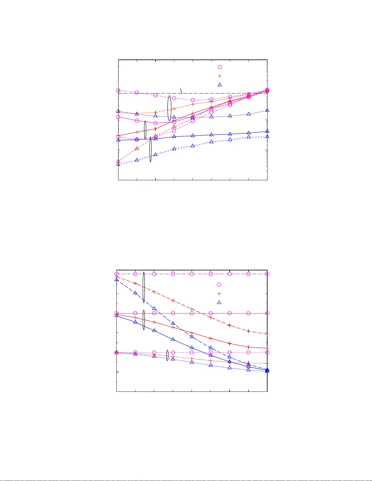
1 Impact of CSI on Distri b uted Space- T ime Cod ing in W ire less Relay Ne tw orks Mari K obayashi, SUPELEC Gif-sur-Yv ette, France Email: mari. kobayashi@s upelec.fr Xa vier Mestre, CTTC Barcelona, Spain Email: xavie r.mestre@ct tc.cat Abstract W e consider a two-ho p wireless network where a transmitter comm unicates with a receiver via M relays with an amplify- and-fo rward (AF) protoc ol. R ecent works ha ve sho wn that sophisticated linear processing such as beamfor ming and distributed space- time coding (DSTC) at relays enables to improve the AF performan ce. Howe ver , the relative utility o f these s trategies dep end on the av ailable channel state in formation at transmitter (CSIT), wh ich in turn depe nds o n sy stem param eters such a s the speed of the un derlying fading channel and that of train ing and feedback proc edures. Moreover , it is of practical interest to hav e a sing le transmit schem e that handles different CSIT scenarios. Th is mo ti vates us to con sider a u nified app roach based on DSTC that potentially provide s diversity gain with statistical CSIT and explo its some additional side inf ormation if av ailable. Und er individual power constrain ts at the relays, we op timize the amplifier power allocation such that pairwise erro r probability conditioned on the av ailable CSIT is m inimized. Under perfect CSIT we prop ose an on- off gradien t algorithm that efficiently finds a set of relays to switch o n. Un der partial and statistical CSIT , we prop ose a simple waterfilling alg orithm that yields a non-tr i vial solution betwee n ma ximum power alloc ation and a gen eralized STC that eq ualizes the a veraged amp lified noise fo r all relay s. Moreover, we derive closed -form solutions for M = 2 and in certain asy mptotic regimes tha t enable an e asy inter pretation of th e pr oposed algorithms. I t is fo und th at an appr opriate am plifier power a llocation is m andator y f or DSTC to o ffer sufficient d iv ersity an d p ower g ain in a gener al ne twork topolo gy . I . M OT I V A T I O N W e con sider a wireless relay ne twork illustrated in Fig.1 where a trans mitter communicates with a receiver via M relays and eac h terminal has a single antenn a. W e let h , g denote the cha nnel vector b etween the transmitter an d the rela ys, the c hannel vector between the relays and the rec ei ver . For its simplicity , we focu s on an amplify-and- forward (AF) protocol [1], [2] in a two-hop commu nication: in the first T ch annel uses the transmitter broadcas ts a codeword, then in the secon d T channe l use s relays amplify and forward the observed c odeword by applying some linear precode r (to be sp ecified la ter). W e assume that a trans mitter an d M relay s have individual power con straints rather than a total power cons traint, since in a p ractical wireless ne twork terminals are ph ysically distributed and hence are subject to their own power supplies . In a classical AF protocol, the amplifier co efficients have be en determined s o as to satisfy required power constraints [1]. In order to improv e the performanc e of the AF p rotocol, a large n umber o f rec ent works have considered so me a dditional linear processing at relays [3], [4], [5], [6], [7], [8], [9], [10]. These works can be roughly classified into two classes according to the ir a ssumption o f c hannel s tate information a t transmitter (CSIT) and the ir objective. The first class assumes perfect CSIT and aims to maximize either the achiev a ble rate or the instantaneou s rec ei ve SNR [3], [4], [5], [6]. The resulting transmit scheme yields beamforming with appropriate power allocation. The second class assu mes only statistical CS IT and a ims to minimize the error prob ability by designing some type of linea r precode r [7], [8], [9], [10]. In p articular , sign ificant attention has been pa id to distrib u ted space -time coding (DSTC) in which each relay sends a dif ferent column o f a S TC matrix [11], [8], [9], [10]. W ith a single antenna at eac h terminal, we has ten to sa y that the go al of DSTC is to ap proach full diversity gain of M of fered by the rela y-receiv er ch annels g since the mu ltiplexing ga in of the MISO chann el under the half-duplex cons traint is very limited, i.e. 1/2. No tice that a n AF bas ed DSTC that ac hiev es the optimal di versity- multiplexing tradeoff [12] has been well studied [13 ], [14], [15 ], [16]. It clearly ap pears that a practical utility of 2 these two app roaches depe nds o n the available CS IT , which in turn depends on the sp eed o f f a ding and tha t of feedback and training procedures . Notice that in a two-hop co mmunication model obtaining pe rfect CSIT is rathe r challenging bec ause the transmitter needs at least a two-step training an d feedba ck proce ss, i.e. first learns h and then g , which typica lly induces ad ditional delay and es timation error . Conseq uently , the perfec t CSIT ass umption holds only if the und erlying fading is quasi-static a nd a su f fi ciently fast feedback and training is av ailable. For this pa rticular cas e, the first approach might be useful. On the con trary , if a rate o f feedback and training is muc h slower than the co herence time of the chann el, the se cond app roach b ased on the statistical cha nnel knowledge is more appropriate. The a bove observation moti vates us to find a unified approach that c an handle different CSIT sce narios, rather than changing a transmit strategy as a function of the quality of side information. T o this end, we fix our transmission strategy to DSTC that potentially provides diversity gain with statistical CSIT and further power gain if a dditional side information is avail able. Our go al is not to fi nd the optimal strategy for each CSIT c ase but to p ropose a unified DSTC sche me tha t simply adapts the amplifier p ower allocation to available CSIT . Among a large family of DSTC, we c onsider linear dispersion (LD) codes [17] b ecaus e they offer desirable pe rformance in terms o f div e rsity gain and c oding gain [10], [18] and mo reover keep the amplified n oise white. The latter con siderably simplifies the power allocation strategy . W e assume perfect s ynchroniza tion between relay terminals and perfect channe l s tate information available at the rec eiv e r , wh ich is nece ssary for c oherent detection. Und er this setting, we will addres s the followi ng que stion: how d oes the quality of CSIT impact the amplifier power alloca tion a nd the resulting performance of the DSTC? T o answ er the que stion, we op timize the a mplifier power allocation in su ch a manner that the pa irwise e rror prob ability (PEP) conditioned on CSIT is minimized. Note that the conditional PEP is a p erformance criteria wide ly use d in the literature o f STC [19], [20], [21] and DSTC [22], [10], [18]. In particular , [21] h as provided elegant preco der d esigns that minimize the PEP cond itioned o n CSIT for orthogon al STC. Unfortunately the extension o f this work to a two-hop relay ne twork appe ars very dif ficult due to the non - con vexity of the u nderlying problem. W e examine the following CS IT cas es : 1) perfect knowledge of the absolute value o f the entries of h and g ( per fect CSIT ), 2) perfect knowledge of absolute v alue of the e ntries of h and statistical knowledge of g ( par tial C SIT ), a nd 3) statistical knowledge of h and g ( statistical CSIT ). Under perfect CSIT , the PEP minimization reduces to the maximization of an a pproximate rec eiv e SNR. The optimal power allocation strategy turns ou t to be a n on-off strategy , whereby so me relays are switched off and others transmit at maximum available power . W e propos e an on -of f gradient algorithm tha t efficiently finds the optimal set of relays to switch on. Under pa rtial an d s tatistical CSIT , the conditional P EP minimization app ears very difficult due to the self-interference caus ed by amplified noise and c alls for a go od h euristic app roximation. First, we a pply a Laplac e-based saddle point a pproximation of an inherent integral in order to make the problem amenable. Since the approx imated problem is still n on-con vex due to av eraged amplified no ises, we transform it into a conv ex problem via a log transformation [23] ass uming a high transmitter power (which is the re gime of interest). For a new objectiv e function, we propose a very simple waterfilling algorithm that yields a no n-tri vial solution be tween ma ximum power a llocation and a g eneralized STC that equalizes the av e raged amplified n oise, i.e. p i γ g ,i with γ g ,i being the variance o f the ch annel between relay i and the rec eiv e r (in a classical STC we consider γ g ,i = 1 , ∀ i ). W e d eri ve clos ed-form solutions for M = 2 a nd in ce rtain asy mptotic regimes that enable an easy interpretation of the propos ed algorithms. It is found that that an approp riate power allocation is manda tory for DSTC in order to provide diversity and power gains in a gene ral network topology . In order to situate this work in the c ontext of rele vant literature, we note that the LD based DSTC for a two-hop AF ne twork has been ad dressed for a single-antenna ca se [10] and for a multiple antenna case [18]. In both works, Jing an d Hass ibi p rovided the diversity an alysis by o ptimizing the power p artition betwee n the transmitter and the relays under the assumptions tha t the transmitter and M relays are subject to a total power cons traint and that b oth channe ls hav e unit variance. Clearly , the o ptimal power partition under this s etting, letting the transmitter u se ha lf of the total p ower a nd each relay sh are the othe r half, does not hold for a g eneral ne twork topology with unequ al variances. W e ma ke a progress with resp ect to this since our proposed waterfilling solution c an b e applied for any set of variances under statistical CSIT and moreover h andles the pa rtial CSIT ca se. W ith perfect CSIT , J ing proposed a c ooperative beamforming sc heme for the same two-hop AF n etwork [5]. Although this beamforming scheme provides a non -negligible power gain comp ared to ou r on-off power a llocation a s shown in Section VI, we remark that our on-of f algorithm is much simpler and can be implemented at the rece i ver without requiring any knowledge at the transmitter . T o this e nd, it suf fic es that the receiver sends to each relay a feedbac k of one 3 bit indicating whe ther to ac ti vate o r not. Henc e, our on-off algorithm might be a ppealing due to its robustness and simplicity despite its suboptimal performance. The res t of the p aper is organized as follows. After briefly introducing the two-hop network model in Section II, we de ri ve the the con ditional PEP upper bo unds for diff e rent CSIT cas es in Section III. In Section IV we propose efficient algorithms that s olve the c onditional PEP minimization, namely on-off grad ient algorithm for perfect CSIT and waterfilling algorithm for partial an d statistical CSIT . W e provide some as ymptotic properties of these algorithms in Section V and numerical examples in Sec tion VI. Fina lly we c onclude the paper in Se ction VII. I I . S Y S T E M M O D E L W e consider frequen cy-flat fading chan nels and let g = [ g 1 , . . . , g M ] T , h = [ h 1 , . . . , h M ] T denote the ch an- nel vector between transmitter and relays, the channe l vector between relays and receiver , respectiv ely . W e as- sume the e ntries of h and g are i.i.d. zero-mean circularly s ymmetric comp lex Gaussian with variance γ h = [ γ h 1 , . . . , γ hM ] , γ g = [ γ g 1 , . . . , γ g M ] respe cti vely . The variance of e ach chan nel is assumed to c apture path-loss a nd shadowing. W e assume a bloc k fading mode l, namely h and g remain c onstant over a block of 2 T channel uses . In this paper we do not con sider a transmitter-r eceiver direc t link for s implicity . It is we ll known however tha t the direct link should be taken into accoun t if one aims at optimizing the di versity-multiplexing tradeoff [13], [14 ], [16], [15]. The communica tion between the trans mitter and the receiv e r is performed in two steps. The trans mitter first broadcas ts a symbol vector s = [ s 1 , . . . , s T ] T ∈ C T × 1 with E [ ss H ] = I T and relay i receives y i = √ p s h i s + n i where p s is the power of the transmitter and n i ∼ N C ( 0 , N 0 I T ) is A WGN. In the second T channel uses, M relays a mplify a nd forward the o bserved codeword by applying a linear preco der . Namely , the transmit vector x i of relay i is giv en by x i = q i A i y i (1) where q i denote a complex amplifier coefficient of relay i , A i ∈ C T × T is a unitary matrix s atisfying A H i A i = I T , and x i should satisfy a power constraint, i.e. E [ || x i || 2 ] = | q i | 2 E [ || y i || 2 ] ≤ T p r where the expec tation is with respect to n i for a short-term constraint and with res pect to both n i and h i for a long-term co nstraint. This in turns impos es a co nstraint on { q i } suc h that | q i | 2 ≤ P i where P i denotes the maximum amplifier power of relay i giv e n b y P i = ( p r p s | h i | 2 + N 0 , short-term p r p s γ hi + N 0 , long-term The received signal a t the fin al destination is gi ven by r = M X i =1 g i x i + w = M X i =1 g i h i q i A i s + M X i =1 g i q i A i n i + w where w ∼ N C ( 0 , N 0 I T ) is A WGN at the receiver uncorrelated with { n i } . The received vector c an be further simplified to r = √ p s SQf + v (2) where we let S = [ A 1 s , . . . , A M s ] ∈ C T × M denote a LD codeword, Q = diag ( q 1 , . . . , q M ) is a diago nal matrix with M amplifier coe f ficients, f = [ h 1 g 1 , . . . , h M g M ] T is a composite c hanne l vector , and we let v = M X i =1 q i g i A i n i + w (3) 4 denote the overall noise whose covariance is gi ven by E [ vv H ] = N 0 M X i =1 | q i | 2 | g i | 2 + 1 ! I T = σ 2 v I T It follows tha t the overall noise see n by the rec eiv e r is white an d this conside rably simplifies the amplifier power allocation in the followi ng sections . I I I . C O N D I T I O N A L P E P W ith p erfect knowledge of b oth h and g , the receiver can perform Max imum Likelihood de coding 1 by estimating a codeword a ccording to ˆ S = arg min S ∈ S || r − √ p s SQf || 2 (4) When the tr ansmitter has only partial k nowledge o f the c hannels , it is reasonable to co nsider the pairwise error probability (PEP) conditioned on the av ailable CSIT . In the following we derive the expre ssions o f the con ditional PEP for three different CSIT ca ses: 1) perfect CSIT , where the trans mitter knows the a bsolute values of the entries of h , g , 2) partial CSIT whe re the transmitter kn ows the absolute values o f the entries of h and γ g , 3) statistical CSIT where the transmitter knows γ h and γ g . Perfect CSIT corresp onds to the c ase of quasi-static fading, while statistical CSIT co rresponds to the c ase of fast fading s o that the transmitter can track only the seco nd order statistics of the ch annel. Finally , partial CSIT is an intermediate ca se relev ant to a time-division duplexing sy stem where the transmitter learns perfectly h by reciprocity but only statistically g due to a low- rate feedbac k. A. P erfect CS IT The PEP cond itioned on h , g for a ny k 6 = l is de fined b y P ( S k → S l | h , g ) ∆ = Pr  || r − √ p s S l QHg || 2 ≤ || r − √ p s S k QHg || 2 | S k , h , g  = Pr  d 2 ( S k , S l ) ≤ κ  where the c omposite chann el f is decoupled into Hg wi th H = diag ( h ) , where we d efine squared Euclidea n distance between S l and S k as d 2 ( S k , S l ) = p s g H H H Q H ( S k − S l ) H ( S k − S l ) QHg and wh ere κ = 2 √ p s Re { v H ( S k − S l ) Qf } is a real Gauss ian rand om variable dis trib uted a s N R (0 , 2 σ 2 v d 2 ) . In order to ob tain a upper boun d of the PEP , we assu me that the term ( S k − S l ) H ( S k − S l ) ha s a full rank M , i.e. the LD code ac hiev e s a full d i versity (for a spec ial c ase of orthog onal STC this always holds). By letting λ min denote the smallest singular value of ( S k − S l ) H ( S k − S l ) over all possible codewords, we o btain the inequality d 2 ( S k , S l ) ≥ p s λ min g H H H Q H QHg which yields a Chernoff bound P ( S k → S l | h , g ) ≤ exp  − p s λ min g H H H Q H QHg 4 σ 2 v  . (5) Minimizing the RHS of (5) correspon ds to maximizing appr oximated rece i ve SNR, g i ven by p s λ min g H H H Q H QHg 4 σ 2 v = η P M i =1 p i | g i | 2 | h i | 2 P M i =1 p i | g i | 2 + 1 (6) where we let η = λ min p s / 4 N 0 and let p i = | q i | 2 denote the amplifier power of relay i . Notice that the above function depends on the absolute values of chan nels and of amplifier coe f ficients. 1 In practice, efficient decoding techniques such as sphere decoding can be implemented to achiev e near ML results [17 ]. 5 B. P artial CS IT The PEP uppe r bou nd con ditioned on h , γ g is obtained by averaging (5) over the d istrib u tion of g P ( S k → S l | h , γ g ) (a) ≈ Z 1 det ( π diag ( γ g )) exp ( − g H η H H PH 1 + P M i =1 γ g i p i + d iag ( γ g ) − 1 ! g ) d g = det η 1 + P M i =1 γ g i p i diag ( γ g ) H H PH + I M ! − 1 = M Y i =1 1 + η | h i | 2 γ g i p i 1 + P M i =1 γ g i p i ! − 1 (7) where in (a) we let P = diag ( p 1 , . . . , p M ) and apply a Laplace-base d saddle point approximation that be comes accurate as the nu mber of relays increase s without boun d (see further Appendix I). This sa ddle point approx imation is inspired by the approximation method sugge sted in [24] to ev alua te the expec tation of quotients of qua dratic forms in Gaussian random variables. W e remark tha t, in o rder to maximize the corresp onding cost function in (7), only the absolute values of the entries of h are nee ded. C. Statistical C SIT The PEP uppe r bou nd con ditioned on γ h , γ g is obtained by averaging (5) over the d istrib u tion of h and g P ( S k → S l | γ h , γ g ) ≤ E g  det − 1  I M + η tr ( G H PG ) diag ( γ h ) G H PG  (a) ≈ E g   M Y j =1 1 + η γ hj | g j | 2 p j 1 + P M i =1 γ g i p i ! − 1   (b) = M Y j =1 1 ρ j e 1 /ρ j E 1 (1 /ρ j ) (c) = M Y j =1 1 ρ j  − γ + ln( ρ j ) + O  1 ρ j  (d) ≈ M Y j =1 1 + P M i =1 γ g i p i η γ g j γ hj p j ln η γ g j γ hj p j 1 + P M i =1 γ g i p i ! (8) where in (a) we apply the La place-bas ed saddle-po int app roximation of the integral mentioned above, (b) follows by noticing tha t | g i | 2 /γ g i is a n exponen tial random variable with unit mean and u sing [25, 3 .352] where we write ρ j = ηγ hj γ gj p j 1+ P M i =1 γ gi p i and let E 1 ( x ) = R ∞ x e − t t dt denote the exponential integral. In (c) we assume that ρ j is large ( η → ∞ ) so that e 1 /ρ j E 1  1 ρ j  = − γ + ln( ρ j ) + ∞ X k =1 ( − 1) k +1 ( ρ j ) − k k k ! = − γ + ln( ρ j ) + O  1 ρ j  where γ is the Euler c onstant, and finally in (d) we assu me ln( ρ j ) ≫ γ . I V . P O W E R A L L O C A T I O N A L G O R I T H M S This sec tion propose s efficient power a llocation a lgorithms to optimize (6), (7 ), and (8). A. P erfect CS IT Under perfect CSIT , the optimal p ⋆ is obtained by maximizing f 0 ( p ) ∆ = P M i =1 α i p i 1 + P M i =1 β i p i (9) where p i is subject to the maximum amplifier power of relay i , i.e. p i ≤ P i = p r p s | h i | 2 + N 0 and we let α i = | h i | 2 | g i | 2 and β i = | g i | 2 . W e rema rk tha t the linear c onstraints form a feasible region V composed by M half-spaces with 2 M − 1 vertices. For M = 2 the feas ible region V is a rectangular region with 3 vertices ( P 1 , 0) , (0 , P 2 ) , ( P 1 , P 2 ) plus the origin. Since this problem is quasi-linear , it is possible to trans form it into a linear program. By exp loiting the s tructure o f the problem, we propos e a more e f ficient algorithm to fin d the solution. First, we start with the follo wing proposition. 6 Proposition 1 The solution to (9) is always found in the on e of 2 M − 1 vertices of the feasible region V . Moreover , at the solution p ⋆ , the entries of the gradient satisfy the follo wing inequality for i = 1 , . . . , M . ∂ f 0 ∂ p i ( p ⋆ )  > 0 , if p ⋆ i = P i ≤ 0 , if p ⋆ i = 0 (10) Proof see Appe ndix II. For M = 2 we have a closed form solution of the optimal power a llocation a s a n obvious res ult of Proposition 1. Corollary 1 For M = 2 , we find a closed-form solution giv en by ( p 1 , p 2 ) =        ( P 1 , 0) , if | h 1 | 2 < p r | g 2 | 2 | h 2 | 2 p s | h 2 | 2 + p r | g 2 | 2 + N 0 (0 , P 2 ) , i f | h 2 | 2 < p r | g 1 | 2 | h 1 | 2 p s | h 1 | 2 + p r | g 1 | 2 + N 0 ( P 1 , P 2 ) , if | h 1 | 2 > p r | g 2 | 2 | h 2 | 2 p s | h 2 | 2 + p r | g 2 | 2 + N 0 and | h 2 | 2 > p r | g 1 | 2 | h 1 | 2 p s | h 1 | 2 + p r | g 1 | 2 + N 0 (11) Proof see Appe ndix III. In order to visua lize the conditions of activ ating relay 1 and/or relay 2 , we provide a graph ical representation of the o n-off region in Fig. 5. Interes tingly , it can be observed there is a minimum value of | h i | 2 in orde r for relay i to be activ ated. Namely relay 1 is activ ated independ ently of relay 2 if | h 1 | 2 > p r p s | g 2 | 2 which is readily obtaine d when letting | h 2 | 2 → ∞ in the first inequality o f the thir d condition, i.e. | h 1 | 2 > p r | g 2 | 2 | h 2 | 2 p s | h 2 | 2 + p r | g 2 | 2 + N 0 , and v ice versa. For M > 2 , the solution d oes not lea d itself to a simple closed form express ion. Ne vertheles s, as a straightforward result of Proposition 1 we propose the followi ng algorithm to solve (9). On-off gradient algorithm 1) Initialize p (0) to an arbitrary vertex ∈ V 2) At iteration n , compu te the gradien ts ∂ f ∂ p ( p ( n ) ) and update p ( n +1) i = h p ( n ) i + ∇ i ( p ( n ) ) i P i 0 , i = 1 , . . . , M (12) where we let ∇ i ( p ( n ) ) = − P i if ∂ f 0 ∂ p i ( p ( n ) ) < 0 and ∇ i ( p ( n ) ) = P i if ∂ f ∂ p i ( p ( n ) ) > 0 , and [ x ] b a denotes the value of x truncated to the interval [ a, b ] . 3) Stop if p ( n ) satisfies (10). Proposition 2 The on-off grad ient algo rithm co n verges to the global maximum. Proof See Appe ndix IV. Fig. 2 plots the con vergence behavior of the propos ed on-off algorithm when we let p s = p r = 10 and conside r equal variances γ h,i = γ g ,i = 1 for a ll i . The objectiv e values are normalized with respe ct to the optimal values and averaged over a lar ge n umber of random channe l realizations. Fig. 2 as well as other examples s how that the proposed on-off gradient algorithm co n verges only after a few iterations irrespe cti vely of M an d of the initialization. It is worth noticing that this on-off algorithm can be implemented at the rec eiv e r without any knowledge at the transmitter . T o this end, it suffices that the receiv e r sen ds to each relay a feedba ck of on e bit indicating whether to activ ate or not. B. P artial CS IT When the transmitter knows h and γ g , the problem reduce s to minimizing (7) or maximizing f 1 ( p ) = M X i =1 ln 1 + η | h i | 2 γ g i p i 1 + P M j =1 γ g j p j ! (13) The term η | h i | 2 γ gi p i 1+ P M j =1 γ gj p j , similar to ρ i = ηγ hi γ gi p i 1+ P M j =1 γ gj p j defined in (b) of (7) for the statistical CSIT ca se, can be interpreted as the c ontrib ution of relay i to the receive SNR. W ith so me abuse o f n otation, we let ρ i denote 7 η | h i | 2 γ gi p i 1+ P M j =1 γ gj p j under partial CSIT . Unfortunately , the func tion f 1 is neither concave or con vex in p . Ne vertheles s, assuming η → ∞ (which is the regime of ou r interest), let u s consider a new objective fun ction, gi ven by J ( p ) = M X i =1 ln a i p i 1 + P j γ g j p j ! (14) where we let a i = η γ g i | h i | 2 for notation simplicity . It is well known that the function J ( p ) can be transformed into a c oncav e function through a log trans formation [23]. In the following, we us e the notation e x to express ln x for any variable x (eq uiv alently x = e ˜ x ). The objec ti ve fun ction c an be expressed in terms of e p as J ( e p ) = M X i =1 ln( a i e e p i ) − M ln   1 + X j exp( e p j ) γ g j   (15) Proposition 3 The optimal e p that maximizes (15) is given ˜ p i = [ ˜ µ ⋆ − ˜ γ g i ] ˜ P i −∞ , p i =  µ ⋆ γ g i  P i 0 (16) where ˜ µ ⋆ is the water level tha t is determined a s follows. Let π de note a p ermutation s uch tha t P π (1) γ g ,π (1) ≤ . . . ≤ P π ( M ) γ g ,π ( M ) . (17) and define ˜ µ j = ln µ j , wh ere µ j is giv e n by µ j = 1 + P j i =1 P π ( i ) γ g ,π ( i ) j j = 1 , . . . , M . (18) The optimal water lev e l ˜ µ ⋆ is obtained as that the value out of these M poss ible one s tha t maximizes the objec ti ve function, namely ˜ µ ⋆ = arg max ˜ µ 1 ,..., ˜ µ M J ( ˜ µ j ) (19) where J ( ˜ µ ) is the o bjectiv e function (15) parame terized by the water level de fined in (31). Proof see Appe ndix V. Fig. 3 illustrates an example of our waterfilling s olution for the cas e M = 3 . The power curve of relay i increases linearly with slope 1 /γ g i and the n is bounde d at its ma ximum amplifier p ower P i . In this example, relays 1 a nd 2 with P i γ g i < µ ⋆ are allocated their ma ximum amplifier powers while relay 3 is a llocated µ ⋆ γ g, 3 . Depending on the water le vel, this waterfilling yields a non-tri vial s olution between maximum power alloca tion ( p i = P i , ∀ i ) and a generalized STC that equalizes the averaged amplified noise p i γ g i = µ ⋆ (notice a classica l STC cons iders γ g i = 1 for all i ). Note that the proposed waterfilling approach only requires a s earch over M values in order to determine the water level, and cons equently it is extremely s imple. Corollary 2 For M = 2 , we find a closed-form solution giv en by ( p 1 , p 2 ) =         1+ P 2 γ g 2 γ g 1 , P 2  , if P 2 γ g 2 ≥ P 1 γ g 1 + 1  P 1 , 1+ P 1 γ g 1 γ g 2  , if P 2 γ g 2 ≤ P 1 γ g 1 − 1 ( P 1 , P 2 ) , otherwise (20) Proof see Appe ndix VI. By expres sing the power constraint P i = p r p s | h i | 2 + N 0 , the above a llocation policy ca n be graphically represe nted as a function of | h 1 | 2 and | h 2 | 2 in Fig. 6. Similarly to Fig. 5 for the cas e of perfect CS IT , there exists a minimum value of | h i | 2 so that rela y i is allocated its maximum a mplifier power . Namely , relay i is allocated its maximum amplifier power inde pende ntly of relay j 6 = i if | h i | 2 > p r γ g,i − N 0 p s . Interes tingly , the thres hold assoc iated to relay i de pends o nly on the i -t h c hannel, as opposed of what ha ppene d in the p erfect CSIT ca se. This mea ns that the power a llocation is more se lfish under pa rtial/statistical CSIT in o rder to inc rease the reliability o f the w ireless link. 8 C. Statistical C SIT When the transmitter only knows the vari ances γ g , γ h of the channels, we minimize the express ion (8) which is equiv ale nt to maximizing f 2 ( p ) = M X i =1 ln η γ hi γ g i p i 1 + P M j =1 p j γ g j ! (21) where w e ignored do ubly logarithmic terms a nd the amplifier p ower p i of relay i is subject to a long-term individual power constraint P i = p r p s γ hi + N 0 for all i . Ag ain, by performing a log-transformation we obtain p recisely the same objectiv e function J ( ˜ p ) in (15) where a i = η γ g i | h i | 2 defined in the pre vious p artial CS IT ca se is replace d with η γ g i γ hi . Hence , the waterfilling solution proposed for the partial CSIT case can be directly applied to the statistical CSIT c ase and ne eds to be implemented once for a giv en set of variances γ h , γ g . Th e power allocation region for M = 2 is gi ven in Fig. 6 where the axes are rep laced b y γ h 1 and γ h 2 . V . A S Y M P T O T I C B E H A V I O R This section s tudies the asymptotic be havior of the propose d power a llocation algorithms and gi ves an informal discuss ion on the resulting error rate performance. A. Relays c lose to transmitter γ h → ∞ W e consider the regime where γ h,i → ∞ or equi valently | h i | 2 → ∞ for all i at the same rate while treating other pa rameters finite. F irst we examine a two re lay ca se. Under prefect CSIT , Fig. 5 implies tha t both relays tend to be switche d on in this regime. Under partial and sta tistical CSIT cas es, it follo ws immed iately from Fig. 6 that two relays s hall transmit at their ma ximum p owers. For M > 2 the same c onclusion can b e drawn as a straightforward result of Proposition 1 for the perfect CSIT case. The condition for which all M relays a re switche d on u nder perfect CSIT is gi ven by | h i | 2 > P M j =1 P j | h j g j | 2 1 + P M j =1 P j | g j | 2 , i = 1 , . . . , M where the RHS corresp onds to the o bjectiv e value f 0 ( P 1 , . . . , P M ) whe n letting all relays transmit with maximum power . The RHS is upper bounde d by f 0 ( P 1 , . . . , P M ) (a) ≤ p r p s P M j =1 | g j | 2 1 + P M j =1 P j | g j | 2 (b) ≤ p r p s M X j =1 | g j | 2 (22) where (a) follo ws from P j | h j | 2 = p r | h j | 2 p s | h j | 2 + N 0 ≤ p r p s and (b) follo ws from 1 1+ P M j =1 | g j | 2 P j ≤ 1 . In the limit of | h j | 2 → ∞ , ∀ j , both (a) and (b) hold with equality and we have | h i | 2 > p r p s M X j =1 | g j | 2 , i = 1 , . . . , M so that all relays are alloca ted the ir maximum powers. From the uppe r b ound (22) of the objective function, it ca n be expected that the performance of distributed LD code improves for a lar ger M . Un der partial and statistical CSIT , the p roposed waterfilling tends to allocate the maximum power to each relay . This ca n be se en immed iately from the waterfilling solution depicte d in Fig.3. As P j → 0 , the values { P i γ g ,i } above which the power curves are bounde d b ecome muc h smaller than the lowest water le vel µ min = 1 / M . This means that all relays are alloca ted the maximum powers. The follo wing remarks are in order; 1) Since the waterfilling a lgorithm un der partial C SIT a nd on-off gradient algo rithm coinc ide, both algo rithms yield the same error performance. This implies that the knowledge o f g has a negligible eff ect on the performance in the regime. 2) As a final remark, the same beh avior can be observed in the followi ng case s. • the transmitter power increase s p s → ∞ . • the variance γ g of the relay-recei ver channe l d ecrease s, i.e. γ g → 0 or equiv alently | g i | 2 → 0 for all i at the same rate. 9 B. Relays get close to receiver γ g → ∞ W e c onsider the regime where γ g ,i → ∞ or eq ui valently | g i | 2 → ∞ for a ll i at the s ame rate. First we examine a two-relay cas e M = 2 . Und er perfect CSIT , it can be o bserved that the thresho ld values p r | g i | 2 p s above which each relay bec omes activ ate d (represented by straight lines in Fig. 5 ) ge t large and the on-off algorithm con verges to relay selection. Similarly , the waterfilling algo rithm a lso ten ds to allocate on ly one relay with ma ximum p ower under partial and statistical CSIT case s as expecte d from Fig. 6. The only exception is a sy mmetric vari ance case γ h, 1 = γ h, 2 . For M > 2 under perfect CSIT , we n ext sho w that the on-off strategy co n verges to single relay selection as | g i | 2 → ∞ , ∀ i . T o see this, firs t o bserve that if the one -of f algorithm choose s only one relay to switch on, it se lects the relay i ⋆ = arg max i | h i | 2 1 + 1 / | g i | 2 P i The objectiv e value is given by (with some abuse o f n otation in the argument of the cost function) f 0 ( P i ⋆ , 0 M − 1 ) = | h i ⋆ | 2 1 + 1 / | g i ⋆ | 2 P i ⋆ ≤ | h i ⋆ | 2 (23) where the inequality ho lds with equa lity for | g i ⋆ | 2 → ∞ . If the o n-of f algorithm a cti vates any arbitrary s et of m > 1 relays, the corresponding objective is upper bounded b y f 0 ( P 1 , . . . , P m , 0 M − m ) = P m i =1 | h i | 2 | g i | 2 P i 1 + P m j =1 | g j | 2 P j < P m i =1 | h i | 2 | g i | 2 P i P m j =1 | g j | 2 P j (a) = m X i =1 θ i | h i | 2 (24) where in (a) we define θ i = | g i | 2 P i P m j =1 | g j | 2 P j with 0 < θ i < 1 and P i θ i = 1 . W e see that the last expression (24) is strictly smaller than (23) for any m and regardless of a se t of relays. This implies that as the relays get close to the receiver , the on-off algorithm con verges to single relay selec tion. The waterfilling algorithm under partial and statistical CSIT lets only one relay transmit with the maximum power as we see in the followi ng. Let us first conside r the permutation π given in (17) so rting relays ac cording to P π (1) γ g ,π (1) < P π (2) γ g ,π (2) < · · · < P π ( M ) γ g ,π ( M ) with s trict ineq ualities. As γ g ,i → ∞ for all i , the possible water lev e l in (18) is rough ly given by µ j ≈ P j i =1 P π ( i ) γ g,π ( i ) j and the le vels tend to be sorted as µ min ≪ µ 1 < µ 2 ≤ · · · < µ M = µ max (25) Notice that the inequ ality µ j < µ j +1 holds if P j i =1 ( P π ( j + 1) γ g ,π ( j +1) − P π ( i ) γ g ,π ( i ) ) > 1 . W e sh ow that the function J is mon otonically d ecreasing for µ 1 ≤ µ ≤ µ M and the optimal water lev e l is always given by µ 1 . W e recall that the deriv ative of J with res pect to ˜ µ in (32) can be expresse d as a function of µ as ∇ J = 1 − M µ 1 + | C ( µ ) | µ + P i ∈ C ( µ ) γ g i P i where we as sumed | C ( µ ) | > 0 . Under the spec ific order o f the water levels given in (25), we c an further express the deriv ative ∇ J j for each interval µ j < µ ≤ µ j +1 for j = 1 , . . . , M − 1 s uch tha t ∇ J j = j ( µ j − µ ) 1 + ( M − j ) µ + P j i =1 γ g ,π ( i ) P π ( i ) Since we have ∇ J j < 0 for any interv al j , it clearly a ppears that the function is monotonically de creasing thus the waterfilling a lgorithm allocates maximum po we r only to the relay π (1) by letting µ ⋆ = µ 1 . In order to have an insight on the e rror rate pe rformance achiev ed by the waterfilli n g letting p i = µ 1 γ gi for all i , we e valuate the approximated receiv e SNR value f 0 . f 0  µ 1 γ g i  = µ 1 P M i =1 | h i | 2 | g i | 2 γ gi 1 + µ 1 P M j =1 | g j | 2 γ gj (a) ≤ P M i =1 | h i | 2 | g i | 2 /γ g i P M j =1 | g j | 2 /γ g j (b) = M X i =1 θ i | h i | 2 (26) 10 where (a) holds with equality as µ 1 → ∞ ( P i γ g i → ∞ for all i ), and in (c) we de fine θ i = | g i | 2 /γ gi P M j =1 | g j | 2 /γ gj with 0 < θ i < 1 and P i θ i = 1 . W e s ee that the final exp ression is domina ted by (23) ac hiev ed by single relay selection under perfect CSIT . The follo wing remarks are in order; 1) The optimal trans mit sc heme in this regime is s ingle relay selection that c hooses rou ghly the relay with the lar gest | h i | 2 . Activ ating more than one relay become s highly subo ptimal due to large amplified noise. 2) The power allocation unde r pa rtial an d s tatistical C SIT is the same and equalizes p i γ g i . 3) As a final remark, the same beh avior can be observed in the followi ng case s. • the relay power increas es p r → ∞ . • the vari ance of the transmitter -relay cha nnel dec reases γ h → 0 . which yield P i | g i | 2 → ∞ unde r perfec t C SIT and P i γ g ,i → ∞ unde r partial and statistical CSIT . V I . N U M E R I C A L R E S U LT S In this section, we provide some numerical results to illustrate the be havior of the proposed po we r alloca tion algorithms. Assuming a ho mogeneo us network, we let p s = p r . W e co nsider B PSK modulation and ge nerate randomly a LD code with M = T drawn from an isotropic distribution. First, we co mpare the propose d on-off algorithm with other sche mes in a sys tem with M = 2 relays and equal variances γ hi = γ g i = 1 for i = 1 , 2 . Fig. 7 shows the block error probability versu s per-relay SNR p r / N 0 with the on-off algo rithm, ne twork b eamforming of [5], and maximum power allocation that lets b oth relays transmit with their peak powers. For a reference we also p lot the performance of our waterfilling algorithm under s tatistical CSIT . W e obse rve that ne twork bea mforming outperforms the on -of f gradient algorithm by roughly 3 dB by exploiting full cha nnel kn owledge and that both sche mes a chieve the same div ersity gain. On the c ontrary , max imum power allocation has a sub stantial performance loss and fails to achieve full diversity ga in. This clearly shows that an appropriate power allocation is ess ential for distributed L D co de to provide diversit y g ain. Next, we exa mine h ow the ne twork topo logy impacts the propo sed p ower allocation a lgorithms an d the resu lting BER p erformance. T o mo del a simple n etwork topology , we consider a u nit transmitter -rece i ver d istance a nd let the transmitter -relay distance varies in the range 0 < r < 1 . The resulting variances are γ hi = 1 /r 2 and γ g i = 1 / (1 − r ) 2 for all i . For the sake of fair c omparison between sy stems with dif feren t M , we assume that the whole network power P is eq ually shared betwe en the transmitter and M relays so tha t p r = P / ( M + 1) . Fig. 8 shows the BER performance of the propo sed power a llocation algorithms with M = 2 , 4 , 6 a nd P / N 0 = 15 dB along with the performance of the direct transmission with a fixed power P . Fig. 9 s hows the averaged allocated power ratio, i.e. P M i =1 E [ p i ( t ) /P i ( t )] , or e quiv alently the ef fec ti ve n umber of relay s. The follo wing remarks are in order: 1 ) As the relays get clos er to the transmitter r → 0 , the transmitter acti vates all relay s with their maximum power . The waterfill ing solution unde r partial CSIT con verges to the on-of f g radient algo rithm in the limit of r → 0 , which implies that the knowledge of g has a negligible impact on the performance. The result agrees we ll with the a nalysis provided in subsection V -A. 2) As the relays ge t closer to the recei ver r → 1 , the optimal strategy activ ates only one relay to limit the amplified n oise. As seen in Fig. 9 the on-off gradie nt algorithm indeed redu ces to relay selection. On the con trary , the waterfilli ng solution equalizes p 1 γ g 1 = · · · = p M γ g M both under partial and statistical CSIT , a nd moreover it conv e r g es to the same error performance indepen dently the number of relay s. Under the giv e n setting where P 1 γ g 1 = · · · = P M γ g M , the waterfilling s olution u nder statistical CSIT lets all rela ys transmit with maximum power . The result is in a good agreeme nt with the ana lysis of sub section V -B. Fig. 10 shows the BER pe rformance versus P / N 0 for M = 2 , 4 , 8 . Here, we randomly choos e the rela y-receiv er distances and let γ g =[0.85, 3.17 , 1.5 0, 1.89, 2.06 , 2.36, 3.19, 3.99]. The trans mitter -relay distance r = 0 . 5 is fixed ( γ hi = 4 for any i ). Co mpared to the direct transmission, DSTC with o ur prop osed power alloca tion algorithms yields signific ant d i versity gain at moderate to high power regime. Moreover , additional CSIT yields a considerab le power gain. V I I . C O N C L U S I O N S W e co nsidered a two-hop wireless ne twork where M relays aid o ne transmitter- receiver pa ir to c ommunicate via DSTC together with the AF protocol. In order to study the impact of CSIT on the des ign and the performance of DSTC, we o ptimized the a mplifier power a llocation unde r individual power cons traints so that the PEP cond itioned to the available CSIT is minimized. Under perfect CSIT we propose d the on-off grad ient algorithm that efficiently 11 finds a subs et of relays to switch on . It turns out tha t this algorithm can b e implemented a t the rece i ver if the rece i ver can s end a one -bit feedba ck to each relay ind icating whether to switch on or not. Un der partial and statistical CS IT we derived a simple waterfilling algorithm that yields a non -tri vial solution between ma ximum power allocation a nd a gen eralized STC that equ alizes the averaged amp lified powers for all relays. Closed-form so lutions were derived for M = 2 and in certain asy mptotic regimes. Namely , when the relays are physically c lose to the transmitter , the on-off algorithm and the waterfilling algorithm coincide and both let all relays transmit with max imum a mplifier powers. When the relay are c lose to the receiver , the on-off algorithm con verges to relay selection in order to minimize the amplified n oise see n by the receiver while the waterfilling equalizes the averaged amplified noise an d becomes highly sub optimal. Th e proposed amplifier power a llocation algorithms were deriv e d for a particular type of linear dispersion STC but can b e extended to more gene ral LD code as we ll as other class es of STC as long as the amplified noise remains white. A P P E N D I X I S A D D L E P O I N T A P P R OX I M A T I O N The objecti ve of t his appendix is t o justify t he approximations (a) in (7) and (8) and to show that the approximation is valid as the number of relays increas es without bo und. Le t us den ote a = g H H H PHg b = 1 + g H Pg W e n eed to ev alua te E h exp  − η a b i = E  exp  − η g H H H PHg 1 + g H Pg  where the expectation is with respe ct to the statistics o f g . First of all, obs erve that we can write exp  − η g H H H PHg 1 + g H Pg  = lim n →∞ X n where X n = n X k ≥ 0 ( − η ) k k !  a b  k . On the other hand, | X n | < n X k ≥ 0 η k k !  a b  k < exp  η g H H H PHg 1 + g H Pg  < exp  η g H H H PHg g H Pg  ≤ exp  η max 1 ≤ j ≤ M | h j | 2  < ∞ Hence, the bound ed con vergence theorem ensu res that we can write E h exp  − η a b i = E h lim n →∞ X n i = lim n →∞ E [ X n ] = X k ≥ 0 ( − η ) k k ! E   a b  k  (27) and we can therefore conc entrate on the study of the moments r k = E   a b  k  . In particular , we can foll ow the proc edure introduce d in [24 ], which is base d on a L aplace a pproximation of the integral. More specific ally , in [24] it was sh own that a La place ap proximation of r k about the origin leads to the identity r k = E "  a E [ b ]  k # + R k (28) 12 where both expec tations are with respe ct to g a nd we have R k → 0 as M → ∞ . Although the procedure is somewhat ted ious, on e can extend this to s how tha t sup k R k → 0 . As a direct cons equenc e of this theorem, we have tha t as M → ∞ , it h olds that 2 E h exp  − η a b i = X k ≥ 0 ( − η ) k k ! E   a b  k  = X k ≥ 0 ( − η ) k k ! E "  a E [ b ]  k # + R k ! = E  exp  − η a E [ b ]  + X k ≥ 0 ( − η ) k k ! R k where now       X k ≥ 0 ( − η ) k k ! R k       ≤ sup k R k exp ( − η ) → 0 and this justifies the approximation used in the paper . A P P E N D I X I I P R O O F O F P RO P O S I T I O N 1 In order to prove Proposition 1, we conside r the i -th entry of the gradient of the objec ti ve function, gi ven by ∂ f 0 ∂ p i = α i + α i P j 6 = i β j p j − β i P j 6 = i α j p j (1 + β i p i + P j 6 = i β j p j ) 2 . When we treat the variables { p j } j 6 = i fixed, the i -th gradient can be expressed as a function of p i in the form ξ i ( β i p i + ζ i ) 2 , where ζ i > 0 and ξ i are c onstants. De pending o n the sign of ξ i , the g radient is a lw ays negati ve or positiv e , i.e. the function is monoton ically d ecreasing o r inc reasing in each p i 3 . Since the objective function canno t be maximized at 0 < p i < P i , the solution of (9) is ach ie ved only at on e of the vertices. The se cond part follo ws directly from the mono tonicity o f the fun ction in ea ch c omponent p i . Namely , the solution is achieved by the vertex at which the objective function ca nnot further inc rease beyond the thresholds . A P P E N D I X I I I P R O O F O F C O RO L L A RY 1 : A C L O S E D - F O R M S O L U T I O N O F M = 2 U N D E R P E R F E C T C S I T From Proposition 1, we see immediately that the power alloca tion of two relays depe nd on the sign of ξ 1 ( p 2 ) = α 1 + ∆ p 2 , ξ 2 ( p 1 ) = α 2 − ∆ p 1 where we let ∆ = α 1 β 2 − β 1 α 2 = | g 1 g 2 | 2 ( | h 1 | 2 − | h 2 | 2 ) . Moreover , it is suf ficient to check the sign of ξ 1 and ξ 2 at each vertex to de termine the optimum p ower alloca tion. T a ble I summa rizes the optimal solution and the co nditions ; the o ptimal solution is giv e n by ( P 1 , 0) if and only if ξ 2 ( P 1 ) = α 2 − ∆ P 1 < 0 holds while it is given by a vertex (0 , P 2 ) if and only if we have ξ 1 ( P 2 ) = α 1 + ∆ P 2 < 0 . Finally , bo th relays are acti vated if − α 1 P 2 < ∆ < α 2 P 1 . Thes e inequalities yield (11). A P P E N D I X I V P R O O F O F P RO P O S I T I O N 2 : C O N V E R G E N C E O F O N - O F F G R A D I E N T A L G O R I T H M W e ha ve to first prov e that the objecti ve is non-decreas ing, i.e. f ( p ( n +1) ) ≥ f ( p ( n ) ) for any iteration n . Identifying that the u pdate in (12) is nothing than a discrete steepe st ascent algorithm with a fixed step size, the objectiv e always inc reases. It remains to prove that the con verged point is the glob al max imum. In other words, the s topping criterion above is s uf ficient to g uarantee a globa l con ver ge nce. It is not difficult to see that there is a unique p ⋆ satisfying the cond ition (10) s uch that the signs of the gradients an d the powers ma tch. Otherwise, we can a lw a ys increase the objective b y s witching on (off) the power with a positive (nega ti ve) grad ient. 2 In t he last equality of the follo wing section, one should justify the fact that expectation and sum can be interchanged . This is not dif ficult to see, but the proof is omitted due to space constraints. 3 For ξ i = 0 , t he f unction is constant in p i , t hen we let p i = 0 . 13 A P P E N D I X V P R O O F O F P RO P O S I T I O N 3 : W A T E R FI L L I N G S O L U T I O N U N D E R PA RT I A L C S I T Since J ( e p ) is a strictly con cave function of e p , we solve the KKT cond itions which are n ecess ary a nd sufficient for optimality . By letting λ i ≥ 0 a La grangian variable as sociated to the individual power constraint p i ≤ P i , we obtain the KKT conditions giv e n by 1 − M γ g i exp( ˜ p i ) 1 + P j γ g j exp( ˜ p j ) = λ i , i = 1 , . . . , M (29) Summing the above equation over all i and defining I = P j γ g j exp( ˜ p j ) and µ = 1 P i λ i we obtain I = M µ − 1 (30) It follows that µ is lower bounde d by µ min = 1 M and uppe r bounde d by µ max = 1+ P j γ gj P j M . Plugging (30) into (29) and using the inequality λ i ≥ 0 , we read ily obtain the optimal power given in (16). It remains to determine the optim al water level ˜ µ ⋆ that maximizes the objecti ve function J (note that the indi v idual power constraint is always sa tisfied for any µ ). T o this end, we define C ( ˜ µ ) and C ( ˜ µ ) as C ( ˜ µ ) = { i | ˜ p i = ˜ µ − ˜ γ g i } , C ( ˜ µ ) = { i | e p i = e P i } Plugging (16) into (15), the function can be expresse d in terms o f ˜ µ J ( ˜ µ ) = | C ( ˜ µ ) | ˜ µ + X i ∈ C ( ˜ µ ) ˜ P i − M ln   1 + | C ( ˜ µ ) | exp ( ˜ µ ) + X i ∈ C ( ˜ µ ) γ g i exp( ˜ P i )   + M X i =1 ln a i (31) where | C | , | C | den otes the cardina lity of the set C , C resp ectiv e ly . Sinc e the func tion J ( ˜ µ ) is strictly concave in ˜ µ , the optimal ˜ µ must sa tisfy ∂ J ∂ ˜ µ = 0 whe re ∂ J ∂ ˜ µ = | C ( ˜ µ ) | 1 − M exp( ˜ µ ) 1 + | C ( ˜ µ ) | exp( ˜ µ ) + P i ∈ C ( ˜ µ ) γ g i exp( ˜ P i ) ! (32) which yields exp( ˜ µ ) = 1 + P i ∈ C ( ˜ µ ) exp( ˜ P i + ˜ γ g i ) | C ( ˜ µ ) | (33) for | C ( ˜ µ ) | > 0 . Notice that for | C ( ˜ µ ) | = 0 , it can be shown tha t the objec ti ve fun ction is a mo notonically increasing concave function a nd maximized at ˜ µ max . By sorting { P i γ g i } in an increasing o rder ac cording to the permutation (17), we remark that the RHS o f (33) h as at most M possible v alues 4 in (18) and we choose the optimal ˜ µ ⋆ according to (19). A P P E N D I X V I P R O O F O F C O RO L L A RY 2 : A C L O S E D - F O R M S O L U T I O N O F M = 2 U N D E R P A RT I A L C S I T W ithout loss o f gen erality , we assume P 1 γ g , 1 < P 2 γ g , 2 . W e recall tha t the possible v alues of the water le vel (18 ) for M = 2 a re µ 1 = 1 + P 1 γ g , 1 µ 2 = µ max = 1 + P 1 γ g , 1 + P 2 γ g , 2 2 . First we conside r the case µ 1 < µ 2 . Th is inequality reduces to P 2 γ g , 2 > P 1 γ g , 1 + 1 , a nd further y ields P 1 γ g , 1 < µ 1 < µ 2 < P 2 γ g , 2 . Obviously w e obta in p 1 = P 1 no ma tter which of the two values is the optimum water level. It is not difficult to see that the op timal water lev el is given by µ 1 by c omparing the two objective values J ( ˜ µ 1 ) and J ( ˜ µ 2 ) . Hence the amplifier power of relay 2 is p 2 = µ 1 γ g 2 = 1+ P 1 γ g 1 γ g 2 . Next we consider the case µ 2 < µ 1 . Th is inequ ality is eq uiv alent to P 2 γ g , 2 < P 1 γ g , 1 + 1 , a nd yields P 2 γ g , 2 < µ 2 . In this case, the water level (either µ 1 or µ 2 ) is lar ger than 4 Some of the M v alues might be unfeasible if they are not in the domain ˜ µ ∈ [ ˜ µ min , ˜ µ max ] . 14 P 1 γ g , 1 and P 2 γ g , 2 . Hence, the a lgorithm lets both relay s transmit a t the max imum p ower , p 1 = P 1 and p 2 = P 2 . In summary , we have the followi ng power allocation pos sibilities: • p 1 = P 1 and p 2 = 1+ P 1 γ g 1 γ g 2 < P 2 if P 2 γ g 2 > P 1 γ g , 1 + 1 • p 1 = P 1 and p 2 = P 2 if P 2 γ g 2 < P 1 γ g , 1 + 1 By symmetry , whe n P 1 γ g 1 > P 2 γ g 2 we obtain • p 1 = P 1 and p 2 = P 2 if P 2 γ g 2 < P 1 γ g , 1 < P 2 γ g 2 + 1 • p 1 = 1+ P 2 γ g 2 γ g 1 < P 1 and p 2 = P 2 if P 1 γ g 1 > P 2 γ g 2 + 1 These c onditions and the co rresponding power alloca tion are summarized in (20) an d depicted in Fig. 4 . Since the parameter P i γ g i does not provide an e asy interpretation (note that P i is a function o f h ), we express the power allocation region in terms of γ g , h explicitly . The subregion where o nly relay 1 , 2 is allocated its maximum power is giv e n respe cti vely by | h 2 | 2 < p r γ g 2  | h 1 | 2 + N 0 p s  p s | h 1 | 2 + p r γ g 1 + N 0 − N 0 p s , | h 1 | 2 < p r γ g 1  | h 2 | 2 + N 0 p s  p s | h 2 | 2 + p r γ g 2 + N 0 − N 0 p s These conditions yield the power allocation region in terms of h in Fig. 6 . A C K N O W L E D G M E N T This work was partially s upported by the Gene ralitat de Catalunya under grant SGR20 05-00690 and by the European Commission under project IST -6FP-033533 (COOPCOM). R E F E R E N C E S [1] J. L aneman, D. Tse, and G. W ornell, “Cooperati ve di versity in wireless netw orks: Ef fi cient protocols and outage behavior, ” IEEE T rans. on Inform. Theory , vol. 50, no. 12, pp. 3062–3080, 2004. [2] J. L aneman and G. W ornell, “Energy-ef fi cient antenna sharing and relaying for wireless networks, ” W ireless Communications and Networking Conferen ce, 2000. WCNC. 2000 IEEE , vol. 1, 2000. [3] I. Hammerstrom, M. Ku hn, and A. W it tneben, “Impact of relay gain allocation on the performan ce of cooperati ve diversity netw orks, ” VTC F all, LA , 2004. [4] A. Wittneben, I. Hammerstrom, and M. Kuh n, “Joint cooperativ e div ersit y and schedu ling in low mobility wireless network s, ” Globecom200 4, Dallas, TX , Nov .-Dec. 2004. [5] Y . Jing and H. Jafarkh ani, “Network Beamforming using Relays with P erfect Channel Information, ” A coustics, Speech and Signal Pr ocessing, 2007. ICA SSP 2007. IEEE International Confer ence on , vol. 3, 2007. [6] Y . Li, B. V ucetic, Z. Zhou, and M. Dohler , “Distributed Adaptiv e Power Allocation f or Wireless Relay Networks, ” W i r eless Communications, IEE E T ransactions on , vol. 6, no. 3, pp. 948–958, 2007 . [7] Y . Ding, J.-K. Zhang, and K. M. W ong, “The Amplify-and-Forward Half-Duplex Cooperativ e System : Pairwise Error Probability and Precoder Design, ” IEEE T rans. on Sig. Pro cessing , vol. 55, no. 2, February 2007. [8] Y . Jing and H. Jafarkhani, “Using Orthogonal and Quasi-Orthogonal Designs in Wireless Relay Net works, ” IEEE T rans. on Inform. Theory , vol. 53, no. 11, pp. 4106–411 8, 2007. [9] G. Scutari and S. Barbarossa, “Distributed S pace-Time Coding for Regenerati ve Relay Networks, ” IEE E T ran s. on W ireless Commun . , vol. 4, S eptember 2006. [10] Y . Jing and B. Hassibi, “Distributed S pace-Time Coding in Wireless Relay Networks, ” IE EE T rans. on W ireless Commun. , vol. 5, December 2006. [11] J. Laneman and G. W ornell, “Di stributed space-time-coded protocols for exploiting cooperativ e di versity in wireless networks, ” IEEE T rans. on Inform. Theory , vol. 49, no. 10, pp. 2415–242 5, 2003. [12] L. Zheng and D. Tse, “Div ersi ty and multiplexing: a fundamen t al tradeof f in multiple-antenna channels, ” Information Theory , IEEE T ransactions on , vol. 49, no. 5, pp. 1073–1096, 2003. [13] R. Nabar , H. Bolcskei, and F . Kneubuhler , “Fading relay channels: performance limits and space-time signal design, ” Selected Area s in Communications, IE EE Journ al on , vol. 22, no. 6, pp. 1099–1109, 2004. [14] K. Azarian, H. Gamal, and P . S chniter , “On the achie vable dive rsity-multiplexing tradeof f in half-duplex cooperati ve channels, ” Information Theory , IEEE T ransactions on , vol. 51, no. 12, pp. 4152–4172, 2005. [15] S. Y ang and J. Belfi ore, “T oward s the Optimal Amplify-and-Forw ard C ooperati ve Diversity Scheme, ” IEEE T rans. on Inform. T heory , vol. 53, no. 9, pp. 3114–3126 , 2007. [16] ——, “Optimal S pace-T ime Codes for the Amplify-and-Forw ard Cooperati ve Channel, ” IEEE T rans. Inform. Theory , vol. 53, no. 2, 2007. [17] B. Hassibi and B. Hochwald , “High-rate codes t hat are linear in space and time, ” IEEE Tr ans. on Inform. Theory , vol. 48, no. 7, pp. 1804–1 824, 2002. [18] Y . Jing and B. Hassibi, “Cooperati ve Dive rsity in Wireless Relay Networks with Multiple-Antenna Nodes, ” submitted to IEE E T rans. on Signal Proce ssing , 2006. 15 [19] V . T arokh, N. Seshadri, and A. Calderbank, “Space-time codes for high data rate w ireless communication: performance criterion and code construction, ” Information Theory , IEEE Tr ansactions on , vol. 44, no. 2, pp. 744–765, 1998. [20] J. Guey , M. Fitz, M. Bell, and W . Kuo, “Signal design for transmitter div ersity wireless communicationsystems ove r Rayleigh fading channels, ” Communications, IEE E T ransactions on , vol. 47, no. 4, pp. 527–537, 1999. [21] G. Jongren, M. Skoglund, and B. Ott ersten, “Combining Beamforming and Orthogonal Space-Time Block Coding, ” IEE E T rans. on Inform. Theory , vol. 48, March 2002. [22] S. Y iu, R. Schober , and L. Lampe, “Distributed Space-T ime Block Coding, ” IEEE T rans. on Commun. , vol. 54, no. 7, pp. 1195–12 06, 2006. [23] M. C hiang, “Geometric Programming for Commun ication Systems, ” F oundations and Tr ends in Communications and Information Theory , vol. 2, no. 1-2, July 2005. [24] O. Lierberman, “A Laplace approximation to the moments of a ratio of quadratic forms, ” B iometrika , vol. 81, no. 4, pp. 681–6 90, 2004. [25] I. Gradshteyn, I. Ryzhik, and R. Romer, “T ables of Integ rals, Series, and Products, ” American Jou rnal of Physics , vol. 56, p. 958, 1988. 16 relay 1 relay 2 relay M source dest. h g Fig. 1. A wireless relay network 0 2 4 6 8 10 12 14 16 18 20 0.2 0.4 0.6 0.8 1 M=4 Iteration averaged normalized objective Impact of M M=8 M=10 M=16 Fig. 2. Con vergen ce of on-of f algorithm for different M p i µ ∗ P 1 P 2 P 3 P 1 r g,1 P 2 r g,2 Fig. 3. Proposed waterfilling solution w ith M = 3 verte x ξ 1 ξ 2 ∆ ( P 1 , 0) + - ( α 2 /P 1 , ∞ ] ( P 1 , P 2 ) + + ( − α 1 /P 2 , α 2 /P 1 ) (0 , P 2 ) - + [ −∞ , − α 1 /P 2 ) T ABLE I O P T I M A L S O L U T I O N S A N D C O R R E S P O N D I N G C O N D I T I O N S 17 P 1 γ g1 1 1 Relay 1 Max Relay 2 < P 2 Relay 1 Max Relay 2 Max Relay 2 Max Relay 1 < P 1 P 2 γ g2 = P 1 γ g1 +1 P 2 γ g2 P 2 γ g2 = P 1 γ g1 −1 Fig. 4. Power allocation region as a function of P i γ gi |h 1 | 2 |h 2 | 2 p r |g 2 | 2 p s Relay 2 ON Relay 1 OFF Relay 2 ON Relay 1 ON Relay 2 OFF p r |g 1 | 2 p s Relay 1 ON Fig. 5. T wo-relay ON/OFF region under perfect CSIT 18 p r γ g1 −Ν 0 p s Relay 1 Max Relay 2 Max Relay 1< P 1 Relay 2 Max Relay 1 Max Relay 2 < P 2 p r γ g2 −Ν 0 p s |h 1 | 2 |h 2 | 2 Fig. 6. T wo-relay po wer region under partial CSIT 10 12 14 16 18 20 22 24 10 −5 10 −4 10 −3 10 −2 10 −1 SNR per relay [dB] Jing’s beamforming M=2 Block error probability Varg = Varh = [1,1] on−off algorithm waterfilling (no CSIT) maximum power Fig. 7. Block err or rate vs SNR 19 0.1 0.2 0.3 0.4 0.5 0.6 0.7 0.8 0.9 10 −5 10 −4 10 −3 10 −2 10 −1 Tx−Relay distance r symbol error rate partial CSIT perfect CSIT SNR=15dB BPSK statistical CSIT M=2 M=4 M=6 direct transmission Fig. 8. BER vs. transmitter-relay distance 0.1 0.2 0.3 0.4 0.5 0.6 0.7 0.8 0.9 0 1 2 3 4 5 6 Tx−Relay distance r Averaged normalized power partial CSIT perfect CSIT SNR=15dB M=6 M=4 M=2 BPSK statistical CSIT Fig. 9. Normalized all ocated power vs. transmitter-relay distance 20 5 10 15 20 25 30 35 10 −5 10 −4 10 −3 10 −2 10 −1 Total power [dB] symbol error rate direct transmission partial CSIT perfect CSIT M=2 r=0.5, γ h =4 M=4 M=8 M=2 M=4 Asymmetric γ g statistical CSIT Fig. 10. BER performance vs P / N 0