The Capacity Region of the Degraded Finite-State Broadcast Channel

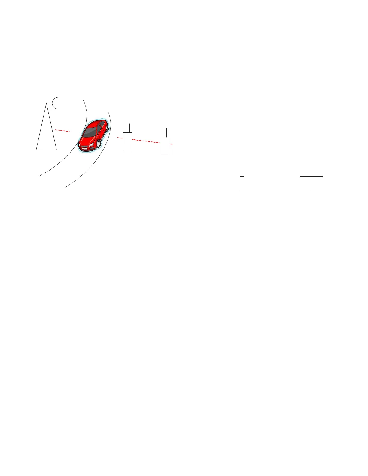
The Capacity Region of the De graded Finite-State Broadcast Channel Ron Dabora and Andrea Golds mith Dept. of Electrical En gineering, Stanford University , Stanford, CA Abstract — W e consider th e discrete, ti me-va rying broadcast channel with memo ry und er the assumption that the ch annel states belong to a set of finite cardin ality . W e first d efine the phys- ically degraded fin ite-state broadcast chann el fo r which we derive the capacity reg ion. W e then define the stoc hastically degraded finite-state broadcast chann el and d eriv e the capacity region f or this scenario as well. In both scenarios we consider the non- indecomposable finite-state channel as well as the indecomposable one. I . I N T R O D U C T I O N The br oadcast cha nnel (BC) was intro duced by Cover in 1972. In this scenario a sin gle sender transmits three messages, one commo n and two priv ate, to two receiv ers over a channel defined b y  X , p ( y , z | x ) , Y × Z  . Her e, X is the cha nnel input from th e transmitter, Y is the channel outp ut at Rx 1 and Z is the ch annel output at Rx 2 . In the years following its introdu ction the study of th e BC fo cused o n memo ryless sce- narios, i.e., when the prob ability of a block of n transmissions is giv en b y p ( y n , z n | x n ) = Q n i =1 p ( y i , z i | x i ) . In recent ye ars, models of time-varying br oadcast channels with memory have attracted a lot of a ttention, especially Gaussian BCs. This was motiv ated by the proliferation o f mobile co mmunicatio ns, fo r which th e chan nel is subject to time-varying co rrelated fading . The correlation of the fading p rocess introduces memory in the BC. The fading BC is on e instance of the g eneral BC with channel states. While fading BCs have recei ved consider able attention, discrete, time-varying BCs with chan nel states have not bee n well studied . A no table exception is the degrad ed arbitrarily varying BC (D A VBC) con sidered in [2] and [3]. In [2] D A VBCs with causal and no n-causal side inform ation at the transmitter were considered . T he states are assumed i.i.d. and the channel is memory less: p ( y n , z n | x n , s n ) = Q n i =1 p ( y i , z i | x i , s i ) . In [3 ], the cap acity region for D A VB Cs with causal side inf ormation at the transmitter and non-cau sal side infor mation at the good rece i ver was deri ved. In [3] the state distribution is gener al and is not subject to th e i.i.d. restriction, b ut the ch annel ou tputs, g i ven the states and the channel inp uts are again m emoryless. T he g eneral, discrete BC with i.i.d. states non -causally known at the transmitter was con sidered in [4]. The arbitr arily varying channe l (A VC ) is on e model for a time-varying chan nel with states. It mod els a mem oryless channel whose law v aries in time in an arbitrary m anner . The state transitions are independ ent of the channe l inpu ts and outputs. In this work we study the discrete time-varying BC with memor y in the f ramew ork of fin ite-state channels (FSCs). The a uthors are wit h the W irele ss Systems Lab, De partment of Electric al E nginee ring, Stanford Uni versi ty , Stanford, CA 94305. Email: { ron,andrea } @wsl.sta nford.edu . This work was supported in part by the DARP A ITMANET program under grant 1105741- 1-TFIND. In con trast to the A VC, in the FSC both th e channe l o utput and th e curren t state depend on both the channel in put and th e previous state. The finite-state ch annel model was used to mo del point-to- point ch annel variations as early as 1953 [1]. This ch annel is characterized by the distribution p ( y , s | x, s ′ ) where S is the current state and S ′ is the previous state. For a b lock of n transmissions, the p.m.f. at the i ’th symbol time satisfies p ( y i , s i | x i , s i − 1 , y i − 1 , s 0 ) = p ( y i , s i | x i , s i − 1 ) , (1) where s 0 is the state of the chan nel when transmission began. Equation (1) implies that S i − 1 contains all the h istory inf or- mation for tim e i . Recently , the fin ite-state mu ltiple-access channel was studied in [6]. This scena rio is characterized by the chann el distribution p ( y , s | x 1 , x 2 , s ′ ) , and the work in [6] also considered the ef fect of feed back on the rates. In the pre sent w ork we study the fin ite-state broadcast channel (FSBC). Here, the channel fro m the transmitter to the receivers is g overned by a state sequence that depe nds on the channel inputs, outp uts an d previous states. The way these symbols inter act with each other is captured b y the transition function p ( y, z , s | x, s ′ ) . Main Con tributions and Organization In this paper we consider for the first time the cap acity of the FSBC. Her e, there is a u nique aspect not encou ntered in the poin t-to-poin t and the MAC coun terparts, namely th e application of superp osition coding to the FSC. W e initially define the ph ysically degrad ed FSBC and find the capac ity region of this scenario. W e then define the stochastically de- graded FSBC and giv e examp les of communication scenarios represented by this mo del. W e der i ve the capacity region for this channel as well. The rest of this paper is organized as fo llows : Section II introdu ces the cha nnel mod el. Section III presents a summar y of the results togeth er with a discussion. Lastly , Section IV outlines the proo f of the capac ity region for the p hysically degraded FSBC. I I . C H A N N E L M O D E L A N D D E FI N I T I O N S First, a word about nota tion. In th e fo llowing we denote random variables w ith upper case letters, e.g. X , Y , and the ir realizations with lower case letters x , y . A rando m variable (R V) X takes values in a set X . W e use ||X || to denote the cardinality of a finite, discrete set X , X n to denote the n -fold Cartesian produ ct of X , and p X ( x ) to denote the prob ability mass function ( p.m.f.) of a discrete R V X on X . For br evity we m ay omit the subscrip t X when it is obvious from th e context. W e use p X | Y ( x | y ) to deno te th e con ditional p.m.f. of X giv en Y . W e den ote vector s with boldface letter s, e. g. x , y ; the i ’th element of a v ector x is denoted with x i and we use x j i where i < j to den ote th e vector ( x i , x i +1 , ..., x j − 1 , x j ) ; x j is sho rt for m notation for x j 1 , and x ≡ x n . A vector of n rando m v ariables is denoted by X n , and similarly we define X j i , ( X i , X i +1 , ..., X j − 1 , X j ) for i < j . W e use H ( · ) to deno te the en tropy of a discrete ran dom variable and I ( · ; · ) to deno te the mutual information b etween two rand om variables, as defined in [7, Chapter 2]. I ( · ; · ) q denotes the mutual infor mation ev aluated with a p.m.f. q on the ran dom variables. Finally , co R denotes the con vex hull of th e set R . Definition 1 : The discrete , fin ite-state b r oadcast chan nel is defined by the tr iplet  X × S , p ( y , z , s | x, s ′ ) , Y × Z × S  where X is th e input sym bol, Y and Z ar e the output symb ols, S ′ is the state of the channe l at the end of the p revious sym bol transmission an d S is the state of the chan nel at the end of the current symb ol tran smission. S , X , Y and Z are discrete alphabets of finite cardina lities. The p.m.f of a block of n transmissions is p ( y n , z n , s n , x n | s 0 ) = n Y i =1 p ( y i , z i , s i , x i | y i − 1 , z i − 1 , s i − 1 , x i − 1 , s 0 ) = n Y i =1 p ( x i | x i − 1 ) p ( y i , z i , s i | y i − 1 , z i − 1 , s i − 1 , x i , s 0 ) ( a ) = p ( x n ) n Y i =1 p ( y i , z i , s i | x i , s i − 1 ) , (2) where s 0 is th e initial chan nel state. He re (a) captu res the fact that g i ven S i − 1 , the symbols at time i are inde pendent of th e past. Definition 2 : The FSBC is called physically de graded if its p.m.f. satis fies p ( y i | x i , y i − 1 , z i − 1 , s 0 ) = p ( y i | x i , y i − 1 , s 0 ) , ( 3a) p ( z i | x i , y i , z i − 1 , s 0 ) = p ( z i | y i , z i − 1 , s 0 ) . (3b) Condition (3a) cap tures the in tuitiv e n otion of degraded ness, namely that Z i − 1 is a degrad ed version of Y i − 1 , thus it does not add infor mation when Y i − 1 is gi ven. Note that in the memory less case this cond ition is n ot necessary as, g i ven X i , Y i is in depende nt of the history . Condition (3 b) follows from the standard notio n of degradedness. Using condition s (3a) an d (3b) we ob tain ( when p ( y n , x n | s 0 ) > 0 ) p ( z n | y n , x n , s 0 ) = p ( z n , y n , x n | s 0 ) p ( y n , x n | s 0 ) = Q n i =1 p ( z i , y i , x i | z i − 1 , y i − 1 , x i − 1 , s 0 ) Q n i =1 p ( y i , x i | y i − 1 , x i − 1 , s 0 ) = Q n i =1 p ( x i | z i − 1 , y i − 1 , x i − 1 ) Q n i =1 p ( z i , y i | z i − 1 ,y i − 1 ,x i ,s 0 ) Q n i =1 p ( x i | y i − 1 , x i − 1 ) Q n i =1 p ( y i | y i − 1 , x i , s 0 ) ( a ) = Q n i =1 p ( x i | x i − 1 ) Q n i =1 p ( z i , y i | z i − 1 , y i − 1 , x i , s 0 ) Q n i =1 p ( x i | x i − 1 ) Q n i =1 p ( y i | y i − 1 , x i , s 0 ) ( b ) = Q n i =1 p ( y i | y i − 1 , x i , s 0 ) Q n i =1 p ( z i | z i − 1 , y i , x i , s 0 ) Q n i =1 p ( y i | y i − 1 , x i , s 0 ) ( c ) = n Y i =1 p ( z i | z i − 1 , y i , s 0 ) , (4) where (a) is because ther e is no fe edback, (b) follows from (3a) and (c) follows from (3b). W e co nclude that when (3) holds, p ( z n | y n , x n , s 0 ) = p ( z n | y n , s 0 ) . Hence, p ( y n , z n | x n , s 0 ) = p ( y n | x n , s 0 ) p ( z n | y n , s 0 ) . (5) Note that (4) shows h ow to obtain p ( z n | y n , x n , s 0 ) in a causal man ner . Also note that Z n is a d egraded version of Y n but still d epends on the state sequence (i.e. degraded- ness does not eliminate the memor y). A special case of the physically degrad ed FSBC occurs when in (3b) it ho lds that p ( z i | x i , y i , z i − 1 , s 0 ) = p ( z i | y i ) . Hence, p ( z n | y n , x n , s 0 ) = p ( z n | y n ) = n Y i =1 p ( z i | y i ) . (6) Equation (6 ) is similar to the d efinition of degradedne ss for the DA VBC used in [2]. Definition 3 : The FSBC is called stochastically degr ad ed if there e xists a p. m.f. ˜ p ( z | y ) such th at p ( z , s | x, s ′ ) = X Y p ( y , s | x, s ′ ) p ( z | y , s, x, s ′ ) = X Y p ( y , s | x, s ′ ) ˜ p ( z | y ) . (7) Note th at wh en ( 7) h olds then p ( z n | x n , s 0 ) = X S n p ( z n , s n | x n , s 0 ) ( a ) = X S n n Y i =1 p ( z i , s i | x i , s i − 1 ) = X S n n Y i =1 X y i ∈Y p ( y i , s i | x i , s i − 1 ) ˜ p ( z i | y i ) = X S n X Y n n Y i =1 p ( y i , s i | x i , s i − 1 ) ˜ p ( z i | y i ) ( b ) = X S n X Y n p ( y n , s n | x n , s 0 ) n Y i =1 ˜ p ( z i | y i ) = X Y n p ( y n | x n , s 0 ) n Y i =1 ˜ p ( z i | y i ) , (8) where (a) and (b) fo llow fro m (2). Definition 3 does n ot constitute only a math ematical co n- venience, but represents a ph ysical scenario . For exam ple, consider a scenario in wh ich a b ase station transmits to two mobile units, loca ted appro ximately on the same line-of- sight from the base station (BS), as indicated by the dashed line in Figu re 1 . Let the BS transm it a BPSK signal and let the r eceiv ed signals be subject to additive Gaussian thermal noise due to th e receivers’ front-en ds. When deco ding at the receivers takes place after a hard thr eshold at z ero, the resulting scen ario is th e bin ary symm etric broa dcast chann el (BSBC). Den ote th e situation where th ere is no traffic on the road between the BS and the mob iles as state A . Let the channel BS–Rx 1 have a crossover pro bability ǫ 1 ( A ) = 0 . 1 and the channel BS–Rx 2 have a crossover probab ility ǫ 2 ( A ) = 0 . 15 . This can be represented as a stochastically degraded BC with a degrading chan nel whose crossover p robability is ǫ 12 ( A ) = ǫ 2 − ǫ 1 1 − 2 ǫ 1 = 0 . 0625 . Assume that o n o ccasions, a car passes on the road between the BS and th e mobiles. Th is causes attenuation in b oth chan nels simultaneou sly . Call this state B and let ǫ 1 ( B ) = 0 . 18 and ǫ 2 ( B ) = 0 . 22 . Again we ha ve ǫ 12 ( B ) = 0 . 0625 1 . Hence, the degrading channel is the same for both states, irrespective of the state sequence (in this examp le the state sequ ence repre- sents the traffic pattern, an d is not an independ ent sequ ence). This satisfies con dition (8). Mobile 1 Mobile 2 Base Station Fig. 1. A degrade d FSBC scenario: the mobile units are located on the same line-of- sight from the base-station (indicated by the dashed line). Passing cars af fect the channel s to both mobile units simultaneo usly . More g enerally , we can define a set of states for this scenario, e. g. S = { 1 , 2 , ..., K } , w ith Y = Z = { 0 , 1 } and p ( z i , s i | y i , s i − 1 ) = p ( s i | s i − 1 ) p ( z i | y i , s i ) p ( z | y , s = k ) =  ǫ 12 ( k ) , z = 1 − y 1 − ǫ 12 ( k ) , z = y , ǫ 12 ( k ) ∈ (0 , 0 . 5 ) , k ∈ S . This results in a co llection of physically degraded BSBCs that ca n g i ve m ore flexibility in modeling th e scenar io of Figure 1, as the degrading channe l may dep end on the state. However , fo r this re ason, this model does n ot satisfy our definition of stochastic degradedness in Definition 3. Definition 4 : (see [5, Section 4.6]) The FSBC is called indecomp osable if for ev ery ǫ > 0 there exists N 0 ( ǫ ) such that for all n > N 0 ( ǫ ) , | p ( s n | x , s 0 ) − p ( s n | x , s ′ 0 ) | < ǫ , for all s n , x , and initial states s 0 and s ′ 0 . Definition 5 : An ( R 0 , R 1 , R 2 , n ) deterministic code for the FSBC con sists of three m essage sets, M 0 =  1 , 2 , ..., 2 nR 0  , M 1 =  1 , 2 , ..., 2 nR 1  and M 2 =  1 , 2 , ..., 2 nR 2  , and three mapping s ( f , g y , g z ) su ch that f : M 0 × M 1 × M 2 7→ X n (9) is th e e ncoder a nd g y : Y n 7→ M 0 × M 1 , g z : Z n 7→ M 0 × M 2 , are the decod ers. Here, M 0 is th e set of com mon m essages and M 1 and M 2 are the sets of private messages to Rx 1 and Rx 2 respectively . 1 The scenario para meters assumed in this example are: T wo-ra y propa- gation model, Rx deco ding scheme is m aximum-lik elihood, Base station Tx po wer = 30 dBm, Base statio n antenna gain = 10 dBi, Rx antenna gain = 0 dBi, Rx noise floor = − 90 dBm, Base station antenna height = 10 m, Rx antenna height = 1 . 5 m, BS–Rx 1 distanc e = 7 . 2 Km and BS–Rx 2 distanc e = 8 Km. W e also assume a passing car increases the path attenuati on by 3 dB. Note that we assume no knowledge of the states at th e transmitter an d r eceivers . Definition 6 : The a verag e pr oba bility of err or of a code for the FSBC is gi ven by P ( n ) e = max s 0 ∈S P ( n ) e ( s 0 ) , where, P ( n ) e ( s 0 ) = Pr  g y ( Y n ) 6 = ( M 0 , M 1 ) o r g z ( Z n ) 6 = ( M 0 , M 2 ) | s 0  , where each of the messages M 0 ∈ M 0 , M 1 ∈ M 1 and M 2 ∈ M 2 is selected indep endently and uniformly . Definition 7 : A rate triplet ( R 0 , R 1 , R 2 ) is called achiev- able for the FSBC if for every ǫ > 0 and δ > 0 there exists an n ( ǫ, δ ) such that fo r all n > n ( ǫ , δ ) an ( R 0 − δ, R 1 − δ, R 2 − δ, n ) cod e with P ( n ) e ≤ ǫ can b e constructed. Definition 8 : The capacity re gion of the FSBC is th e c on- vex hull of all achie vable rate triplets. I I I . M A I N R E S U LT S A N D D I S C U S S I O N Define first R 1 ,n ( p, s 0 ) , 1 n I ( X n ; Y n | U n , s 0 ) p − log 2 ||S || n R 2 ,n ( p, s 0 ) , 1 n I ( U n ; Z n | s 0 ) p − log 2 ||S || n . The main result is stated in the following the orem, wh ose proof is outlined in Section IV: Theor em 1: Let Q n be the set of all joint d istrib utions on ( × n i =1 U i , X n ) such that the car dinality of the random vecto r U n is bou nded by || × n i =1 U i || ≤ min {||X || , ||Y || , ||Z ||} n . F or the physica lly degr ad ed FS BC o f Definition 2, define the r e gion R n ( s 0 ) as R n ( s 0 ) = co [ q n ∈Q n  ( R 0 , R 1 , R 2 ) : R 0 ≥ 0 , R 1 ≥ 0 , R 2 ≥ 0 , R 1 ≤ R 1 ,n ( q n , s 0 ) , R 0 + R 2 ≤ R 2 ,n ( q n , s 0 )  . (10 ) The ca pacity r egion of the physically degraded F SBC is given by C pd = lim n →∞ \ s 0 ∈S R n ( s 0 ) , (11) and the limit e xists. Since the cap acity of th e broad cast channel depends only on the cond itional marginals p ( y n | x n , s 0 ) and p ( z n | x n , s 0 ) (see [7, Chapter 14.6]) then the capacity re gion of the stochastically degraded FSBC is th e same as the cor respondin g physically degraded FSBC: Cor ollary 1 : F or the stochastically d e graded FSBC of Def- inition 3, the capacity re gion is given by Theo r em 1 where p ( z | s , y , x, s ′ ) is r eplaced by ˜ p ( z | y ) that sa tisfies equa tion (7) . When the FSBC is inde composable , th en the e ffect of the initial state fades away as n increases. T herefore we have the following corollar y: Cor ollary 2 : F or the indecomposa ble p hysically de graded FSBC, the cap acity r e gion is given b y Theorem 1. F or the indecomp osable stoc ha stically de graded FSBC, the capac ity r e gion is obta ined fr om Cor ollary 1. In both cases the param- eter s 0 in R 1 ,n ( q n , s 0 ) and R 2 ,n ( q n , s 0 ) and th e intersection over S in the expr ession fo r C pd ar e omitted. Pr oof o utline: Lo osely speak ing, the co rollary is true since for n large eno ugh the ef fect of the initial state fades away . Therefo re, f or asymp totically large n the ma ximum over all initial states s 0 ∈ S equa ls the minimum. Discussion First, n ote that if lim n →∞ R n ( s 0 ) exists for all s 0 ∈ S then the capacity region (1 1) can be wr itten as C pd = lim n →∞ \ s 0 ∈S R n ( s 0 ) ( a ) = \ s 0 ∈S lim n →∞ R n ( s 0 ) . Here, (a) is permitted because S is finite. Thus, the ca pacity region can be v ie wed as the intersection of all the capacity regions o btained when the initial state is known at the recei vers (but no t at th e transmitter). W e also n ote the f ollowing conclusion s: 1) Sin ce the limit of th e region exists, then as n increases, optimizing the code will r esult in b etter p erforma nce ( which is not g uaranteed when the limits cannot be shown to exis t , consider for example a non- stationary chann el with noise that oscillates with time). 2) The codeb ook structure that achieves capacity is a superpo sition codebook. This introduce s a structural constrain t when optimizin g the code book fo r achieving the max imum rate triplets. 3) Th e auxiliary R V U n introdu ces d ifficulties mainly in places where we need to r ely on the its cardinality . This is because we cannot translate the bound on the cardina lity of U n into a boun d o n the cardinality o f a subset of U n . In particular, we can not u se the cardinality of U n when deriving the cap acity region for the inde composable FSBC. Mo reover , letting n = m 1 + m 2 , then from Equation (1) we have that p ( z m 1 , y m 1 , s m 1 | x n , s 0 ) = p ( z m 1 , y m 1 , s m 1 | x m 1 , s 0 ) . But because p ( x m 1 | u n ) 6 = p ( x m 1 | u m 1 ) th en p ( z m 1 , y m 1 , s m 1 | u n , s 0 ) 6 = p ( z m 1 , y m 1 , s m 1 | u m 1 , s 0 ) . This is a major dif feren ce from the po int-to-po int and the MA C channels. Con sider , for example, the expression max p ( u n ,x n )  max s 0 ∈S 1 n I ( U n ; Z n | s 0 ) + λ max s ′ 0 ∈S 1 n I ( X n ; Y n | U n , s ′ 0 )  . (12) While in the MA C and th e point-to-poin t chan nels the corre- sponding expressions conver ge for all channels, f or th e FSBC (12) can be shown to converge o nly fo r the indecomposable case. Th erefore, using superposition codin g, th e cha nnel be- tween U n and ( Y n , Z n ) is fun damentally different fro m the channel b etween X n and ( Y n , Z n ) . This is in contrast also to the discrete, memoryless BC. I V . P RO O F O U T L I N E In the deriv ation we fo cus o n the ph ysically de grad ed FSBC. The der i vation r equires on ly that c ondition (5) holds. In the deriv ation we sh all consider only the two private messages case as the c ommon m essage can be inco rporated by splitting the rate to Rx 2 into priv ate and commo n rates, as in [7, Theorem 14.6.4]. R 1 R 2 s A =1 =1 =0 =0 Achievable Region s B Fig. 2. Line s bounding the achie va ble regions for the FSBC for initial states s A and s B , and the resulting regi on of positiv e error exponent s. A. Achievability Theo r em Due to space limitation s we omit the details of the achiev- ability proof an d g i ve only th e conclusion. For complete details see [8]. Define first F n ( λ ) = max p ( u n ,x n )  min s 0 ∈S R 2 ,n ( p, s 0 ) + λ min s ′ 0 ∈S R 1 ,n ( p, s ′ 0 )  . Follo wing [9, Section 2 ], the b oundar y of the region of positive error expo nents for a given n ca n be written as R n 2 ( R n 1 ) = inf 0 ≤ λ ≤ 1 n F n ( λ ) − λR 1 o . (13) This ch aracterization is illustrated in Figure 2. In the ach iev ability p roof we show that fo r a given p ( u n , x n ) , when tr ansmitting at the po sitive rate pair  min s ′ 0 ∈S R 1 ,n ( p, s ′ 0 ) , min s 0 ∈S R 2 ,n ( p, s 0 )  , then the erro r exponent is positive an d bound ed aw ay from zero. Hence, the probab ility of error c an be made less than any arbitrar y ǫ > 0 by taking a block leng th K n with a large enou gh integer K . Furthermo re, in section IV -D we show that the largest region is o btained by taking the limit R 2 ( R 1 ) = inf 0 ≤ λ ≤ 1  lim n →∞ F n ( λ ) − λR 1  , (14) and that this limit exists and is fin ite. The fact that the limit exists and is finite imp lies that we can appro ach the rates of Theorem 1 arbitrarily close by taking n large enou gh, thus by Definition 7 these rates are achiev able. Before considering the con verse we discuss the cardinality of th e aux iliary R V U n , as the evaluation o f R n 2 ( R n 1 ) o f (1 3) depend s on th e existence of such a b ound. B. Car dinality Bounds From the deriv ation in [ 9], it follows that max imizing the region R n ( s 0 ) of Eq uation (10) over all joint distributions p ( u n , x n ) , can b e carried o ut while the c ardinality of the auxiliary r andom v ariable U n is b ounded by || × n i =1 U i || ≤ min {||X || , ||Y || , ||Z ||} n . (15) Now note th at fro m (11), the ach ie vable region fo r a fixed n is gi ven by the in tersection T s 0 ∈S R n ( s 0 ) . As for each R n ( s 0 ) , s 0 ∈ S we have the same cardin ality bound , then this boun d also holds for maxim izing the in tersection of the regions R n ( s 0 ) , s 0 ∈ S . C. Con verse Lemma 1 : If for some ǫ > 0 , λ ≥ 0 , R 2 + λR 1 > lim n →∞ F n ( λ ) + ǫ, then ther e exists a pair of initial states s 0 and s ′ 0 such that P ( n ) e 2 ( s 0 ) R 2 + λ  P ( n ) e 1 ( s ′ 0 ) R 1  > ǫ − 1 n (1 + λ )(1 + lo g 2 ||S || ) . The implicatio n of this inequality , as explained in [9, Section 3], is th at for n large enou gh th e prob ability o f erro r P ( n ) e cannot b e made arbitrar ily small outside the region (14). Pr oof: From F ano ’ s inequality we have that H ( M 2 | Z n , s 0 ) ≤ P ( n ) e 2 ( s 0 ) nR 2 + 1 (16a) H ( M 1 | Y n , s 0 ) ≤ P ( n ) e 1 ( s 0 ) nR 1 + 1 . (16b) Next write min s 0 ∈S I ( M 2 ; Z n | s 0 ) = nR 2 − ma x s 0 ∈S H ( M 2 | Z n , s 0 ) (17) min s ′ 0 ∈S I ( M 1 ; Y n | M 2 , s ′ 0 ) = nR 1 − max s ′ 0 ∈S H ( M 1 | Y n , M 2 , s ′ 0 ) ≥ nR 1 − ma x s ′ 0 ∈S H ( M 1 | Y n , s ′ 0 ) . (18) Now note th at I ( M 2 ; Z n | s 0 ) = H ( Z n | s 0 ) − H ( Z n | M 2 , s 0 ) = I ( U n ; Z n | s 0 ) , (19) where U i = M 2 , i = 1 , 2 , ..., n . W e also have I ( M 1 ; Y n | M 2 , s ′ 0 ) = H ( Y n | M 2 , s ′ 0 ) − H ( Y n | M 1 , M 2 , s ′ 0 ) ≤ H ( Y n | U n , s ′ 0 ) − H ( Y n | X n , U n , s ′ 0 ) = I ( X n ; Y n | U n , s ′ 0 ) , (20) where the definition of U n satisfies the Markov relationship U n | s ′ 0 − X n | s ′ 0 − Y n | s ′ 0 . Com bining (19) and (20) we have that for this choice of U n : min s 0 ∈S I ( M 2 ; Z n | s 0 ) + λ min s ′ 0 ∈S I ( M 1 ; Y n | M 2 , s ′ 0 ) ≤ min s 0 ∈S I ( U n ; Z n | s 0 ) + λ min s ′ 0 ∈S I ( X n ; Y n | U n , s ′ 0 ) ≤ nF n ( λ ) + (1 + λ ) lo g 2 ||S || , (21) since F n ( λ ) is obtained by maximizin g over all joint distribu- tions p ( u n , x n ) subject to the car dinality constraint (1 5), which is also satisfied by our choice of U n . Let s 0 ,n and s ′ 0 ,n be the maximizing states for H ( M 2 | Z n , s 0 ) and H ( M 1 | Y n , s ′ 0 ) respectively . Plugging (17) and (18) in to (2 1) yields nR 2 − H ( M 2 | Z n , s 0 ,n ) + λ ( nR 1 − H ( M 1 | Y n , s ′ 0 ,n )) − (1 + λ ) log 2 ||S || ≤ nF n ( λ ) . Thus, H ( M 2 | Z n , s 0 ,n ) + λH ( M 1 | Y n , s ′ 0 ,n ) + (1 + λ ) lo g 2 ||S || ≥ n ( R 2 + λR 1 − F n ( λ )) ≥ n ( R 2 + λR 1 − lim n →∞ F n ( λ )) > nǫ . Combined with (16), this comple tes the proof of the lem ma. D. Con ver gence In this subsection we show th at lim n →∞ F n ( λ ) exists and is finite for the channel und er consider ation, when λ ∈ [0 , 1] . The pro of o f conver gen ce extends the arguments in [5, Append ix 4A] to the FSBC. The ma in difficulty her e is the introdu ction of the auxiliar y R V U n and its intera ction with the other R Vs, S n , X n , Y n and Z n . W e actually sho w th at lim n →∞ F n ( λ ) = sup n F n ( λ ) which implies that the limit exists. Due to its leng th, th e full proof is omitted and on ly the main po ints are highligh ted. Let s 0 = s z 0 ( l ) minimize 1 l I ( U l ; Z l | s 0 ) and s ′ 0 = s y 0 ( l ) min imize 1 l I ( X l ; Y l | U l , s ′ 0 ) , for the triplet  q 1 ( u l , x l ) , s z 0 ( l ) , s y 0 ( l )  that achiev es the max -min solutio n for F l ( λ ) , and let ( q 2 ( u m , x m ) , s z 0 ( m ) , s y 0 ( m )) achieve the max-min solutio n F m ( λ ) . Finally , let s z 0 ( n ) an d s y 0 ( n ) b e the states that achie ve the max -min solution f or F n ( λ ) . W e show that F n ( λ ) is sup-add iti ve, i.e., for every integer m, l ∈ [0 , n ] with n = m + l we ha ve nF n ( λ ) ≥ l F l ( λ ) + mF m ( λ ) . Sup-add iti vity is verified by br eaking the length n expres- sions into expr essions of length l and expressions of length m . Th e critical pa rt her e is to consider th e length m sequen ce from l + 1 to n . Here we u se th e fact that giv en th e in itial state the chan nel is stationar y , so p ( Z n l +1 , Y n l +1 | x n l +1 , s l = s 0 ) = p ( Z m 1 , Y m 1 | x m 1 = x n l +1 , s 0 ) . This, combined with the fact th e cardinality bou nd d epends only on th e length of th e sequence, leads to the con clusion that the joint distribution q 2 ( u m 1 , x m 1 ) that maximize s F m ( λ ) will maximize the segment fr om l + 1 to n (i.e. is the m aximizing distribution fo r ( U n l +1 , X n l +1 ) , with the same initial state). Additionally , bo th 1 n I ( U n ; Z n | s 0 ) and 1 n I ( X n ; Y n | U n , s ′ 0 ) are b ounded fr om ab ove, ind ependen t o f n : 1 n I ( U n ; Z n | s 0 ) ≤ log 2 ||Z || , since all the Z i ’ s are defined over the same alphabet Z i ≡ Z , a nd similarly 1 n I ( X n ; Y n | U n , s ′ 0 ) ≤ log 2 ||X || . Thus, F n ( λ ) ≤ lo g 2 ||Z || + λ log 2 ||X || < ∞ for any λ ∈ [0 , 1] . The fact that F n ( λ ) is bound ed f rom above indepe ndent of n and is also sup-ad ditiv e implies that lim n →∞ F n ( λ ) exists and is finite. Combining the fact that the limit exists with sectio ns IV -A, IV -B an d IV -C gives the capacity of the FSBC of Th eorem 1. R E F E R E N C E S [1] B. McMil lan. “The Basi c Theorems of Informatio n Theory”. The Annals of Mathe matical Statistics , V ol-24(2): 196–219, 1953. [2] Y . Steinberg. “Coding for the Degraded Broadcast Cha nnel W ith Random Parameter s, W ith Ca usal and Noncausal Side Info rmation”. IEEE Tr ans. Inform. Theory , IT -51(8):2 867–2877, 2005. [3] A. W inshtok and Y . Steinb erg. “The Arbitra rily V arying Degrade d Broadca st Channel with States Known at the Encoder”. Internati onal Symposium on Information Theory (ISIT) 2006, Seattle , W A, pp. 2156– 2160. [4] Y . Steinberg and S. Shamai. “ Achiev able Rates for the Broadcast Channel with States Kno wn at the Transmitte r”. Pr oc. of the Int. Symp. Inform. Theory (ISIT) 2005, Adelaide , Australi a, pp. 2184–218 8. [5] R. G. Gallager . Information Theory and Reliable Communication. John W iley and Sons Inc., 1968. [6] H. Permuter a nd T . W eissman. “Capacit y Region of the Finit e-State Multipl e Access Channel with and without Feedback”. Submitted to the IEEE Tr ans. Inform. Theory , 2007. [7] T . M. Cov er and J. Thomas. Elements of Information Theory . John W iley and Sons Inc., 1991. [8] R. Dabora and A. Goldsmith . “The Capacity Region of the Degrad ed Finite- State Broadcast Channel ”. Submitted to the IEEE Tr ans. Inform. Theory , 2008. [9] R. G. Gallager . “Capacity and Coding for Degrade d Bro adcast Cha n- nels”. Pr oblemy P er edac hi Informatsii , vol. 10(3):3–14, 1974.