Tight Bounds on the Capacity of Binary Input random CDMA Systems

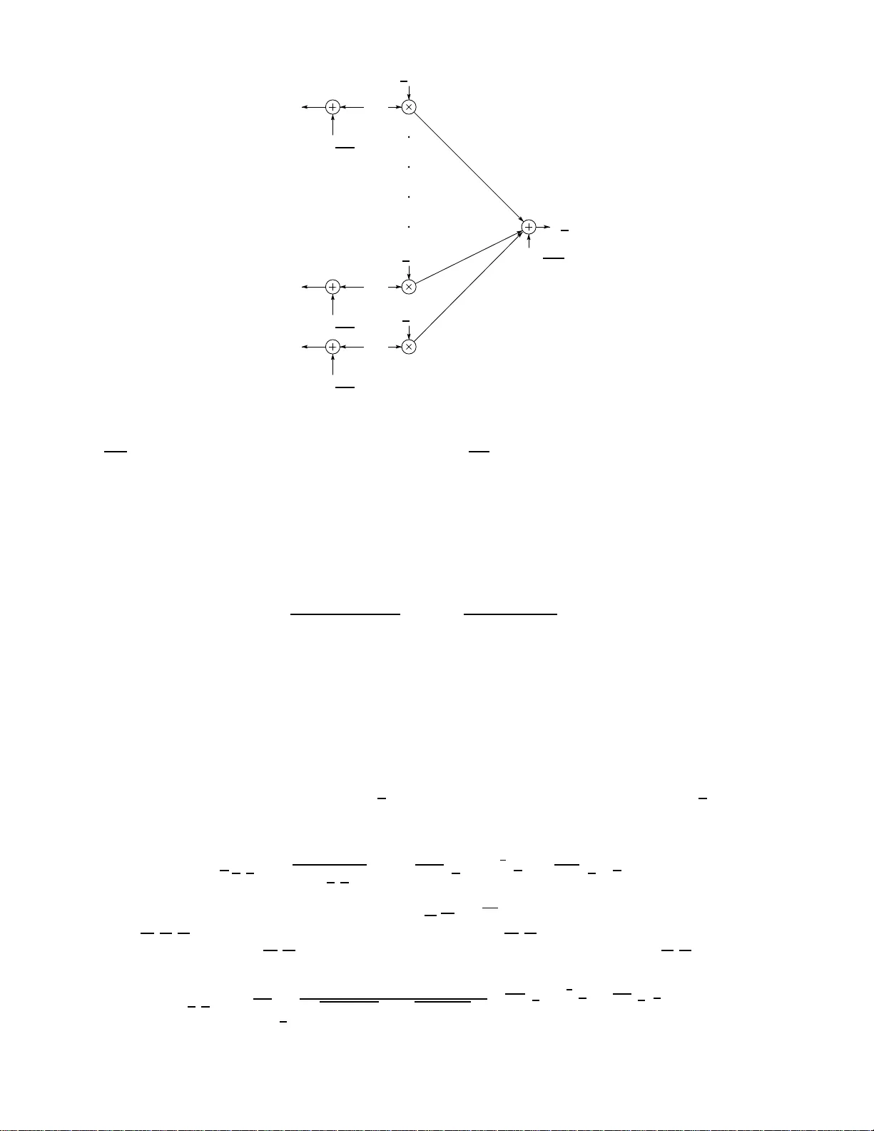
Tigh t Bounds o n the Capacit y of Binary Inpu t random CDMA Systems Satish Babu Korada and Nicolas Macris Sc ho ol of Information and Comm unication Sciences Ecole P olytec hnique F´ ed ´ erale de Lausanne L THC-IC-Station 14, CH-1015 Lausanne Switzerland Octob er 25, 2018 Abstract W e consider multiple access communicatio n on a binary input additive white Gaussian noise channel using randomly spread code div ision. F or a general class of symmetric distributions for spreading coeﬃcients, in th e limit of a large num b er of users, we prov e an up p er b ound on th e capacit y , which matc hes a formula that T anak a obt ained b y using the re plica meth o d. W e also sho w concentration of v a rious relev an t quantitie s including m utual informati on, capacit y and free energy . The mathe- matical metho ds are quite general and al low us to discuss extensions to other multiuser scenarios. 1 In tro duction Co de Division Multiple Access (CDMA) has b een a successful scheme for reliable communication betw een m ultiple us ers and a common re c e iver. The scheme co nsists of K users mo dulating their information sequence by a signature seq uence, also known as spreading sequence, of length N and tr a nsmitting. The num ber N is sometimes referred to as the spr eading gain o r the num b er o f chips p er sequence. The rece iver o btains the sum of all tr a nsmitted signals and the noise which is assumed to be white and Gaussian (A W GN). The achiev a ble rate regio n (for real v alued inputs) with pow er constraints a nd optimal deco ding ha s bee n g iven in [1]. There it is shown that the achiev able rates dep end o nly on the c o rrelatio n matrix of the spreading co eﬃcients. It is w ell known that these detectors ha ve expo nent ial (in K ) complexit y . Therefore, it is imp or tant to a na lyze the p erformanc e under sub-optimal but low-complexity detectors like the linear detectors . F or a g o o d overview of these detectors we r efer to [2 ]. In [3], the authors considered r andom spreading (s pr eading seq uences a re chosen r andomly) and analyzed the sp ectral eﬃciency , deﬁned a s the bits p er chip that can b e r eliably transmitted, for these detectors. In the lar ge- system limit ( K → ∞ , N → ∞ , K N = β ) they obtained nice analytical fo r mulas for the sp ectral eﬃciency and show ed that it concent ra tes. These formulas follow from the known sp ectrum of large co v a riance matrices. In [4],[5] the a uthors analyzed the signa l to interference r atio fo r the de c orrela to r and the MMSE receiv er and sho wed that it is a symptotically Gauss ian with v ariance g oing to zero. Now conside r the cas e where the user input is res tr icted to take o nly binary v alues. Not muc h is known in this case e x cept for the spectra l eﬃciency in the cas e of high SNR which is a na lyzed in [6]. The r andom matrix techniques used for Gaussian inputs do not apply her e b ecaus e the sp ectra l eﬃciency ca nnot b e written in terms of just the cov a riance matrix of the spr eading sequence s. T anak a [7] applied the formal r e plic a metho d, developed in statistical mec hanics, to this problem and conjectured the formula for sp ectra l eﬃciency a nd bit error rate (BER) for unco ded transmis s ion. Thes e results were later extended in [8] to include the case of unequal p ow ers and channel with fading. The replica metho d is non- rigoro us but be lie ved to yield exact res ults for some mo dels in statistical mechanics [9]. Mo re recently Mon tanari and Tse [1 0] hav e made progress to wards a rigoro us deriv ation o f T a nak a’s capa c it y formula in a restricted range of para meters. 1 Our main cont ributions in this paper are t wofold. First we prove that T anak a’s formula is an upper bo und to the capa city for all v a lues of the para meters and second we pr ov e v a rious useful co ncentration theorems in the large-system limit. 1.1 Statistical Mec hanics Approach There is a na tural connection betw een v a rious co mm unication systems and statistical mechanics of random spin systems, stemming from the fact that often in b oth s y stems there is a lar ge num be r of degrees of freedo m (bits o r spins), in terac ting lo cally , in a r andom environment. So far, there hav e bee n a pplications of tw o imp orta n t but s omewhat co mplement ary approaches o f statistica l mechanics of random systems. The ﬁrst o ne is the v ery imp or tant but mathematically uncontrolled replica metho d. The merit of this a pproach is to obtain co njectural but rather explicit for mulas for quantities of interest suc h as, free energy , conditio nal entropy or erro r proba bilit y . In some cases the natur al ﬁxed p oint structure embo died in th e mean ﬁeld for mulas allows to guess goo d iterative algo rithms. This program has b een carried out for linear er ror corr ecting co des, source co ding, m ultiuser settings lik e broa dcast channel (see for e xample [11], [1 2], [13]) and the cas e of interest here [7]: rando mly spread CDMA with binar y inputs. The second t yp e of approach aims at a rigor ous understanding of the r eplica for mulas and has its origins in metho ds stemming from mathematical ph ysics (see [1 4, 15], [9]). F or systems whos e underlying degrees of freedom have Gaussian distribution (Gaussian input sym b ols or Gaus s ian spins in contin uous spin systems) random matrix metho ds can succes s fully be employed. How ever when the degrees of freedom are binary (binary infor mation symbols or Ising spins) these see m to fail, but the rece ntly developed interp olation metho d [14],[15] has had so me success 1 . The ba sic idea of the in terp olation metho d is to study a measure which interp o lates b etw een the poster ior measure o f the ideal dec o der a nd a mean ﬁeld measure. The later can be guessed from the replica f or mulas and from this p er sp ective the replica metho d is a v alua ble to ol. So far this progr am has b een dev elop ed only for linear erro r co rrecting co des o n spar se g r aphs and binary input symmetric channels [16], [17]. In this pap er we develop the interpo lation metho d for the rando m CDMA sy s tem with binary inputs (in the lar g e-system limit). The situation is qualitatively diﬀerent than the ones mentioned ab ov e in that the “underlying g r aph” is complete. Superﬁcia lly one might think that it is similar to the Sherrington- Kirkpatrick mo del which was the ﬁrst one treated by the in ter po lation metho d. How e ver a s we will see the analy s is of the randomly spread CDMA system is substantially diﬀerent due to the structure of the int era c tio n b etw een degr ees of freedom. 1.2 Comm unication Setup W e co nsider a scenario where K users s end binary information symbols x = ( x 1 , . . . , x K ) t , x k ∈ {± 1 } to a c o mmon receiver, thro ug h a single A W GN c hannel. Each us er k has a random signature s equence s k = ( s 1 k , ..., s N k ) t where the comp onents are independently identically distributed. F or each time division (o r chip) interv al i = 1 , ..., N the received sig nal y = ( y 1 , ..., y N ) is y i = 1 √ N K X k =1 s ik x k + σ n i where n = ( n 1 , ..., n N ) t are independent identically dis tr ibuted Ga ussian v ariables N (0 , 1 ) so that the noise p ow er is σ 2 . The v aria nce of s ik is set to 1 and the scaling factor 1 / √ N is introduced so that the power (p er sy m b ol) of each user is norma lized to 1. Our results hold for the rather wide class of distributions s atisfying: Assumption A. The distribution p ( s ik ) is symmetric p ( s ik ) = p ( − s ik ) and has a r apid ly de c aying tail. Mor e pr e cisely, ther e exist s p ositive c onstants s 0 and A such t hat ∀ s ≥ s 0 p ( s ik ≥ s ) ≤ e − As 2 1 Let us p oint out that, as will b e sho wn later in this pap er, the inte rp olation method can also serve as an alternative to random matrix theory for Gaussian i nputs. 2 In particular , o ur fav orite Gaussian and binary cases ar e included in this cla s s, and a lso any compactly suppo rted dis tr ibution. An insp ection of our pro o fs suggests that the results could b e extended to a larger class satisfying: Assumption B. The distribution p ( s ik ) is symmetric with ﬁnite se c ond and fourth moments. How ever to keep the pro ofs as simple as p ossible o nly one of the theorems is prov en with suc h genera lity . In the sequel w e use the notations s for the N × K matrix ( s ik ), S for the corre s po nding ra ndom matrix, a nd X , Y for the input and output random v ectors. Our main in terest is in pro ving a “tight ” upp er bo und o n C K = 1 K max p X E S [ I ( X ; Y )] (1) in the large-s ystem limit K → + ∞ with K N = β ﬁxe d. In the next few paragra phs w e discuss v arious settings for which it is justiﬁed to consider this for mula as a ca pacity . In principle for m ultiaccess channels one max imizes ov er pro duct distributio ns p X ( x ) = Q K k =1 p k ( x k ). But in fac t this restriction makes no diﬀerence when one maximizes the exp ected m utual information because the maxim um is attained for a uniform distribution. Indeed fo r a n y given s the mutual information I ( X ; Y ) is a concav e functional of p X and th us so is its av er age. Moreover t he later is inv aria nt under the tra nsformations p X ( x 1 , x 2 , ..., x K ) → p X ( ǫ 1 x 1 , ǫ 2 x 2 , ..., ǫ K x K ) whe r e ǫ i = ± 1. Co mbining these tw o facts we deduce that the ma ximum in (1) is attained f or the convex co m bination 1 2 K X ǫ 1 ,...,ǫ K p X ( ǫ 1 x 1 , ..., ǫ K x K ) = 1 2 K which is nothing els e than the pr o duct o f uniform distributions for ea ch user. Before discuss ing the meaning of (1 ) for the CDMA setting let us note tha t it can a lso b e interpreted as the c apacity of a MIMO system with binary constellatio ns, K transmit, N receive a ntennas, and erg o dic channel co eﬃcients s ik that are known to the receiver only [18], [19]. In the tr aditional CDMA se tting (see for exa mple [2]) the spreading sequences ar e assigned to each user a nd do not change from sym b ol to sym b ol. Moreov er it is assumed that the user s and the receiver know s . The gener al analysis of multiaccess channels implies that the total capa c it y p er user (or maxima l achiev a ble sum rate) is 1 K max Q K k =1 p k ( x k ) I ( X ; Y ) (2) where the maximum is ov er p i ( x ) = p i δ ( x − 1) + (1 − p i ) δ ( x + 1) and p i ∈ [0 , 1], i = 1 , ..., k . In the large-s ystem limit w e are able to pr ov e a concentration theo rem for the mutual information I ( X ; Y ) which implies that if ( p 1 , ..., p K ) belo ngs to a ﬁnite discrete set D with cardina lit y increasing at mo st po lynomially in K , then (2) concentrates on 1 K max p ∈D E S [ I ( X ; Y )]. Of cour se b y the s a me argument as b efore this maximum is attained f or p = 1 2 as long a s 1 2 ∈ D . Unfortunately , in order to extend these arguments to the more realistic c a se of expone ntial car dinality of D , o r even all possible cont inuous v alues of the input distribution (and thus to fully justify (1)) we would have to pro ve stronger for ms of concentration. A t this point it is interesting to discus s the situatio n for the contin uous input case . The r e it is k nown that the maximum of (2) is attained for a Ga ussian input distribution indep endent o f the spr eading sequence rea lization [1 ]. Then the conce ntration theorems for I ( X ; Y ) suﬃce to prove that in the la r ge- system limit (2) asymptotically equa ls (1). It is an o pen problem to decide if an analogous result holds in the binary input case, namely that the maximum of (2) is attained for the uniform distribution. W e conjecture tha t this is the case. Alternatively , following [3] one may consider the case of “ lo ng sprea ding sequences”, that is seq ue nc e s that extend over many sym b ol durations. Then by “ergo dicity” one can compute the capacity as an exp ectation of (2) ov er S . In the co nt inuous input cas e it turns out that one can switch the exp ectation and the maximum b eca use it can b e shown (b y the standar d a rgument adapted a bove for the binary case) that t he maxim um of the expectatio n is attained for the same Gaussia n input distr ibution. Thus, remark ably , in the contin uo us c ase one exchanges the exp ectation ov er S with the max im um ov er pro duct distributions e ven for ﬁnite K . Finally let us return to the binary c a se and consider the situa tion of long spreading sequences as in [3] that are assumed to b e unknown (or rather not used) to the enco der and known to th e receiver. 3 Then, by the ana lysis in [18], formula (1) gives the capacity . If user s do not co op erate p X is really a pro duct distribution. But in any case t he maxim um is attained for the unifor m distribution. Let us no w collect a few formulas that will b e useful in the sequel. The conditional entrop y H ( X | Y ) = E Y | s [ H ( X | y )] is the average ov er Y giv en s of the Shannon entrop y for the po sterior distribution p ( x | y , s ) = p X ( x ) Z ( y , s ) exp  − 1 2 σ 2 k y − N − 1 2 s x k 2  (3) with the normalization fa ctor Z ( y , s ) = X x p X ( x ) e − 1 2 σ 2 k y − N − 1 2 s x k 2 (4) Note that this is the distr ibutio n used by the ideal or optimal detector. The av era ge over Y is carried out with the distribution induced by th e c hannel transition probability p ( y | s ) = X x 0 p X ( x 0 ) e − 1 2 σ 2 k y − N − 1 2 s x 0 k 2 ( √ 2 π σ ) N = 1 ( √ 2 π σ ) N Z ( y , s ) (5) where in the sum x 0 is in ter preted a s the input signal. The no rmalization fac to r (4) can b e interpreted as the partition function of interacting Ising spins x k = ± 1 with free measur e p X . In v iew of this it is not surprising that the free e ne r gy f ( y , s ) = 1 K ln Z ( y , s ) (6) plays a cr ucial r ole. In appendix A we show that it is r elated to the mutual informa tio n by 1 K I ( X ; Y ) = − 1 2 β − E Y | s [ f ( y , s )] (7) Therefore C K = − 1 2 β − min p X E Y , S [ f ( y , s )] (8) Of course b y the previous discussion the min p X is attained for p X ( x ) = 1 2 K . 1.3 T ana k a’s form ula for bina ry inputs By using the formal replica trick of statistical mechanics T anak a reduced the ca lculation of the conditional ent ro py to a v ar ia tional proble m. His co njectur a l for mula is lim K →∞ C K = min m ∈ [0 , 1] c RS ( m ) (9) where the “replica sy mmetric capacit y functional” c RS ( m ) = λ 2 (1 + m ) − 1 2 β ln λσ 2 − Z D z ln(2 cosh( √ λz + λ )) (10) with λ = 1 σ 2 + β (1 − m ) (11) and D z the standar d Gauss ian measure D z ≡ e − z 2 2 √ 2 π dz , has to be maximize d ov er a par ameter 2 m . I t is easy 3 to see that the maximizer must sa tisfy the ﬁxed p oint condition m = Z D z tanh( √ λz + λ ) (12) 2 this parameter can b e in terpreted as the expected v alue of the MM SE estimate for the information bi ts 3 using integration by parts formula for Gaussian r andom v ar iables 4 The for mal calculations in volved in the replica metho d make clear that the formula (9) should not dep end on the distribution of the spreading sequence (see [7]). In t he present problem o ne exp ects a priori that replica symmetr y is not br oken b e c ause o f a gauge symmetry induced by channel s ymmetry . F or this reaso n T anak a ’s form ula is co njectured to b e ex a ct. Our upper b ound (Theo r em 6) on the capacity precisely coincides with the above fo rmulas and strongly suppo rts this conjecture. Recent work announced b y Mo ntanari and Tse [10] a lso pr ovides strong supp or t to the conjecture at least in a reg ime of β without phase transitions (mor e precisely , for β ≤ β s ( σ ) where β s ( σ ) is the maximal v a lue of β such that the solution o f (1 2) remains unique). The autho rs ﬁr st solve the cas e of sparse signa ture sequence (using the a rea theorem and the da ta pro cess ing inequa lity) in the limit K → ∞ . Then the dense signature sequence (whic h is of interest here) is reco vered by exc hanging the K → ∞ and spar se → dense limits. 1.4 Gaussian inputs In the c a se of contin uous inputs x k ∈ R , in formulas (4), (5) P x are replaced b y R dx . The capa c ity is maximized by a Gaussian pr ior, p X ( x ) = e − || x || 2 2 (2 π ) N/ 2 (13) and one ca n express it in terms of a determinant inv o lving the corr elation matrix of the spr eading sequences. Using the exact s pe c tral measure given by ra ndom matrix theory Shamai a nd V erdu [3] obtained the rigoro us result lim K →∞ C K = 1 2 log(1 + σ − 2 − 1 4 Q ( σ − 2 , β )) + 1 2 β log(1 + σ − 2 β − 1 4 Q ( σ − 2 , β )) − Q ( σ − 2 , β ) 8 β σ − 2 (14) where Q ( x, z ) =  q x (1 + √ z ) 2 + 1 − q x (1 − √ z ) 2 + 1  2 On the other hand T anak a applied the forma l replica method to this case and found (9) with c RS ( m ) = 1 2 log(1 + λ ) − 1 2 β log λσ 2 − λ 2 (1 − m ) (15) where λ = ( σ 2 + β (1 − m )) − 1 . The maximizer sa tisﬁes m = λ 1 + λ (16) Solving (16) we obtain m = σ 2 4 β Q ( σ − 2 , β ) and substituting this in (1 5) gives the equality betw een (14) and (15). So at least for the ca se of Gaussian inputs we ar e already assured tha t the replica metho d ﬁnds t he correct solutio n. As w e will show in section 7.3 our metho ds also work in the cas e of Gaussian inputs, and yield the upper b ound. 1.5 Con tributions and organization of this w or k The main fo cus and challenge o f this work is on the c a se of binar y inputs for the communication set up describ ed a bove, a lthough the metho ds a lso work for m any other constellatio ns including Gaussian inputs. The ma in results are e x plained in section 2 while the remaining sections a r e devoted to the pro ofs. W e prov e concentration of the mutual informa tion in the limit o f K → + ∞ and β = K N ﬁxed (Theorems 1, 3 in section 2.1). As we will see the mathematical underpinning of this is the concentration of a more fundamen tal ob ject, namely , the “free energy” of the asso cia ted spin sys tem (Theorem 2). In 5 fact this turns out to b e imp or tant in the pro o f of the bo und on capac ity . When the spreading co eﬃcients are Gaussian the main to ol used is a p owerful theorem [9] of the concentration of Lips chit z functions of man y indep endent Gaussia n v ariables , and this lea ds to s ubex po nential concentration b ounds. F o r more general spreading coeﬃcient distributions such tools do not suﬃce and we ha ve to combine them with martinga le arguments which lead to weak er algebr aic bounds. Since the concentration pro ofs are mainly technical they are pr esented in app endices B, C. Sections 3 and 4 form the core of the paper . They detail the pro of of the main Theo rem 6 announced in section 2.4, na mely the tigh t upp er bo und on capacit y . W e use ideas from the interpo lation method combined with a non-trivial co ncentration theorem for the empirica l average o f s oft bit estimates. Section 5 shows that the a verage capacity is independent of the spreading sequence dis tr ibution at least for the case where it is symmetric and decays fast enough (Theorem 4 in section 2.2). This enables us to restric t o urselves to the cas e of Gaussian spreading sequences which is more amenable to analysis . The existence of the limit K → ∞ for the capacit y is shown in sectio n 6. Section 7 discusses v a rious extensions of t his work. W e sketch the trea tmen t for unequa l p ow e r s for each user as well a s co lored noise. As alluded to b efor e the b ound on ca pacity for the case of Gaussian inputs c a n als o be obtained by the presen t metho d and w e giv e some indications t o this eﬀect. The appendice s contain the pro ofs of v ario us tec hnical calcula tio ns. Prelimina ry v ersions of the results obtained in this pap er have been summarized in references [2 0] a nd [21]. 2 Main Results 2.1 Concen tration In t he case of a Gaussian input signal, the concentration can be deduced from gener al theor ems o n the concentration of the sp ectra l density for r andom matrices, but this approa ch breaks down for binary inputs. Her e w e pro ve, Theorem 1 ( concen tration of capacit y , Gauss ian spreading sequence, binary inputs). Ass u me the distribution p ( s ik ) ar e standar d Gaussians. Given ǫ > 0 , ther e exists an inte ger K 1 = O ( | ln ǫ | ) indep endent of p X , such that for al l K > K 1 , P [ | I ( X ; Y ) − E S [ I ( X ; Y )] | ≥ ǫK ] ≤ 3 e − α 1 ǫ 2 K wher e α 1 = 1 16 σ 4 (64 β + 32 + σ 2 ) − 1 . The mathematical underpinning o f this result is in fact a more general concentration result for the free ener gy (6), that will b e of some use latter on. Theorem 2 ( concen tration of free energy , Gaussian spreading sequence, binary inputs.). Assume the distribution p ( s ik ) ar e standar d Gaussians. Given ǫ > 0 , ther e ex ists an int e ger K 2 = O ( | ln ǫ | ) indep endent of p X , such that for al l K ≥ K 2 , P [ | f ( y , s ) − E Y , S [ f ( y , s )] | ≥ ǫ ] ≤ 3 e − α 2 ǫ 2 √ K wher e α 2 = 1 32 σ 4 β 3 2 (2 √ β + σ ) − 2 . W e prove these theorems thanks to pow erful probabilistic to ols develop ed b y Ledoux and T alagr and for Lipschitz functions of ma n y Gaussian rando m v aria bles. These to ols are brieﬂy revie wed in App endix B for the conv enience of the reader and the pro o fs of the theorems a re presented in App endix C. Unfortunately the sa me tools do not apply directly to the case of other spr eading sequences. How ever in this case the follo wing w eaker result ca n at leas t b e obtained. Theorem 3 ( concen tration, gene ral spreading sequence). A s s ume the spr e ading se quenc e satisﬁ es assumption B. Ther e exists an inte ger K 1 indep endent of p X , such that for al l K > K 1 P [ | I ( X ; Y ) − E S [ I ( X ; Y )] | ≥ ǫK ] ≤ α K ǫ 2 P [ f ( y , s ) − E Y , S [ f ( y , s )] | ≥ ǫ ] ≤ α K ǫ 2 for some c onstant α > 0 and i ndep endent of K . 6 T o prov e such estima tes it is eno ugh (b y Chebyc heﬀ ) to control second moments. F o r the mutual information we simply hav e to a da pt martingale arguments of P astur, Scherbina and Tirrozzi, [2 2, 23] whereas the case of free energy is more co mplica ted b eca use of the additional Gaussian noise ﬂuctuations. W e deal with these by combining martingale argument s and Lipsc hitz function techniques. The concentration of capacity , namely P [ | max p X I ( X ; Y ) − max p X E S [ I ( X ; Y )] | ≥ ǫK ] ≤ α K ǫ 2 (17) would follow from a stronger (uniform concent ratio n with r esp ect to p X ) P [max p X | I ( X ; Y ) − E S [ I ( X ; Y )] | ≥ ǫK ] ≤ α K ǫ 2 (18) T o see this it s uﬃces to no te that for tw o p os itive functions f and g we have | max f − max g | ≤ max | f − g | . But unfortunately it is not clear how to extend our pro ofs to obtain (1 8). How ever a s announced in the int ro duction we can deduce (18 ) fr o m our theorems, by using the unio n b ound, as long as the maximum is car ried o ut ov er a ﬁnite set (suﬃcien tly small with respect to K ) of distributions. W e wis h to ar gue here that Theor e m 2 suggests a metho d for proving the concentration of the bit error rate (BER) for uncode d communication 1 2 (1 − 1 K K X k =1 x 0 ,k ˆ x k ) (19) where the MAP bit estimate for unco ded communication is deﬁned through the marginal of (3), namely ˆ x k = arg max x k = {± 1 } p ( x k | y , s ). W e remark that ˆ x k = s ig n h x k i where we ﬁnd it convenien t to adopt the sta tistical mec hanics notation h−i for the average with resp ect to the poster ior measure (3). F or example the a verage h x k i = X x x k p ( x | y , s ) (a soft bit estimate or “ma gnetization”) can b e obtained fro m the free ener gy by adding ﬁrst an in- ﬁnitesimal perturbation (“small external magnetic ﬁeld”) to the exp onent in (3), namely h P K k =1 x 0 k x k , and then diﬀerentiating the perturb ed free energy 4 , 1 K K X k =1 x 0 k h x k i = lim h → 0 d dh 1 K ln Z ( y , s ) How ever one really needs to relate sign h x k i to the deriv ative of the free energy and this does not app ear to b e ob vious. O ne wa y out is to in tr o duce pro duct measures of n copies (a lso called “real replicas” ) of the p o s terior mea s ure p ( x (1) | y , s ) p ( x (2) | y , s ) . . . p ( x ( n ) | y , s ) and then relate K X k =1 ( x 0 k h x k i ) n = K X k =1 h x 0 k x 1 k ...x 0 k x n k i n to a suitable deriv ative of the replica ted fr ee energy . Then from the set of all momen ts one ca n in principle r econstruct sign h x k i . Thus one co uld try to deduce the concentration o f the BER from the one for the fr e e energy . How ever the completion of this pro gram r equires a uniform, with resp ect the sys tem size, control of the deriv ative of the free ener gy precisely a t h = 0 , whic h at the momen t is s till la cking 5 . 4 we do not w rite explicitly the h dependence in the per turbed free energy 5 ho wev er this can be done for Lebesgue al most eve ry h 7 2.2 Indep endence with resp ect to the distribution of the spreading sequence The replica metho d leads to the sa me T anak a formula for general class of symmetric distr ibutions p ( s ik ) = p ( − s ik ). W e are able to prove this: in particular bina r y a nd Ga ussian sprea ding s e quences lead to the same capa city . Theorem 4. Consider CDMA with binary inputs and assume A for t he spr e ading s e quenc e. L et C g b e the c ap acity for Gaussian spr e ading se quenc es (symmetric i.i.d with unit varianc e). Then l im K → + ∞ ( C K − C g ) = 0 This theorem turns out to b e v ery useful in order to obtain the b ound o n capa city b ecaus e it allows us to make use of conv enient integration b y parts iden tities that hav e no clear counterpart in the no n- Gaussian case. The pr o of of th e theorem is giv en in section 5 . 2.3 Existence of the limit K → + ∞ The in ter p o lation metho d can b e used to sho w the existence o f the limit K → + ∞ fo r C K . Theorem 5 . Consider CDMA with binary input s and assume A for the spr e ading se quenc es with uniform input distribution. Then lim K →∞ C K exists (20) The pro of of this theorem is given in section 6 for Gaussian spreading sequences . The gener al case then follows b eca use o f Theorem 4. 2.4 Tigh t upp er b ound on the capacit y The main r esult of this pap er is tha t T anak a’s for mu la (10) is an upp er bo und to the capacity for all v alues of β . Theorem 6. Consider CDMA with binary inputs and assume A fo r t he spr e ading se quenc e. We have lim K →∞ C K ≤ min m ∈ [0 , 1] c RS ( m ) (21) wher e c RS ( m ) is given by (10). If w e combine this result with an inequality in Montanari and Tse [10], and exchanging as they do the limits o f K → + ∞ and spar se → dense , one can deduce that the equality holds for some re gime of noise smaller than a c r itical v alue. This v a lue cor resp onds to the thre s hold for belief propag ation deco ding. Note that this equality is v alid even if β is such tha t there is a phase transition (the ﬁxed po int equatio n (12) ha s many solutions ), whereas in [10] the equality ho lds for v a lues of β for which the phase tr ansition do es not occur. Since the pro of is rather complica ted we ﬁnd it useful to g ive the ma in ideas in an informal wa y . The int egr a l term in (10) suggests th at we can replace the o riginal system with a simpler system where the user bits are sent thro ugh K indepe ndent Ga ussian channels g iven b y ˜ y k = x k + 1 √ λ w k (22) where w k ∼ N (0 , 1) and λ is an eﬀectiv e SNR. Of course this argument is a bit naive b eca use this eﬀective system do es not a ccount for the extra terms in (10), but it ha s the merit of identifying the correct interp olation. W e in tro duce an interp o lating pa rameter t ∈ [0 , 1 ] suc h that the independent Gaussian channels corres p o nd to t = 0 and the o riginal CDMA system co rresp onds to t = 1 (see Fig ure 2 .4) It is conv enient to denote the SNR of the original Ga ussian channel as B (that is B = σ − 2 ). Then (11) becomes λ = B 1 + β B (1 − m ) 8 s K x K s 2 x 2 s 1 x 1 N (0 , 1 B ( t ) ) y N (0 , 1 λ ( t ) ) N (0 , 1 λ ( t ) ) N (0 , 1 λ ( t ) ) ˜ y 1 ˜ y 2 ˜ y K Figure 1: The information bits x k are transmitted throug h the norma l CDMA channel with v ariance 1 B ( t ) and thro ugh individual Gaussian channels with noise 1 λ ( t ) W e in tro duce tw o in ter po lating SNR functions λ ( t ) and B ( t ) such tha t λ (0) = λ, B (0) = 0 and λ (1) = 0 , B (1) = B (23) and B ( t ) 1 + β B ( t )(1 − m ) + λ ( t ) = B 1 + β B (1 − m ) (24) The meaning of (24) is the following. In the interpolating t -system the eﬀectiv e SNR seen by each user has an eﬀective t -CDMA pa rt and an indep endent channel part λ ( t ) chosen such that the total SNR is ﬁxed to the eﬀective SNR o f the CDMA system. There is a whole class of interpolating functions satisfying the ab ov e conditions but it turns out tha t we do not need to sp ecify them mo r e precisely except for the fact tha t B ( t ) is increasing, λ ( t ) is decreasing and with contin uous ﬁr s t der iv atives. Subsequent calculations a re indep endent of the par ticular choices o f functions. The par ameter m is to b e c o nsidered as ﬁxed to a ny ar bitrary v alue in [0 , 1]. All the subsequent calculations a re indep endent of its v alue, w hich is to b e optimized t o tigh ten t he ﬁnal b ound. W e now hav e tw o sets of channel outputs y (from the CDMA with noise v ariance B ( t ) − 1 ) and ˜ y (from the independent c hannels with no ise v ar iance λ ( t ) − 1 ) and the interpola ting comm unication system has a p oster ior distribution p t ( x | y , ˜ y , s ) = 1 2 K Z ( y , ˜ y , s ) exp  − B ( t ) 2 k y − N − 1 2 s x k 2 − λ ( t ) 2 k ˜ y − x k 2  (25) Note that here we take without loss of g enerality p X ( X ) = 1 2 K . By ana lyzing the mutual info r mation E S [ I t ( X ; Y , ˜ Y )] of the interpolating system we can r elate E S [ I ( X ; Y )] (the t = 1 v alue) to the easily computed entrop y E S [ I 0 ( X ; ˜ Y )] o f the indep endent channel limit. The average ov er ( Y , ˜ Y ) is now per formed w ith resp ect to p t ( y , ˜ y | s ) = 1 2 K X x 0 1 ( p 2 π B ( t ) − 1 ) N ( p 2 π λ ( t ) − 1 ) K e − B ( t ) 2 k y − N − 1 2 s x 0 k 2 − λ ( t ) 2 k ˜ y − x 0 k 2 (26) These equa tions co mpletely deﬁne the interpo lating co mm unication system. 9 In order to c arry out this program successfully it turns out that w e need a concentration result on empirical a verage o f the “magnetization”, m 1 = 1 K K X k =1 x 0 k x k which, as explained in section 2.1, is closely related to the B E R. Informally speaking we need to prove that the ﬂuctuations o f E h| m 1 − E h m 1 i|i are small. This in volv es the control of tw o types of ﬂuctuatio ns, E h| m 1 − h m 1 i|i a nd E |h m 1 i − E h m 1 i| (by the triang le inequality). In s ome spin glass pro blems b oth t yp e of ﬂuctuations need not be sma ll at the same tim e. Indeed it is a quite gener al fact that the ﬁr st one is s mall for thermo dyna mic (or c onv exity) reasons while the smallness of th e second is not assur ed if replica symmetry breaking o ccurs (see [9]). Her e we use a crucial ingr edient that is sp eciﬁc to the communication set up, namely the channel symmetry , w hich induces a ga uge s y mmetry and preven ts replica brea king. This, it turns out, allows to prove that b oth ﬂuctuations a re small. The control of these ﬂuctuations is the ob ject of Theorem 7 in section 3.3. Ther e are tec hnica l complications that we hav e to dea l with b ecause s uch con trol o f ﬂuctuations is only p os sible awa y fro m phase transitio ns. F o r this reaso n we ha ve to add small appropr iate p ertur ba tions to the measur e (25 ) a nd give almost sure statements with resp ect to the strength of the perturba tion. By being suﬃcien tly careful with the orde r of limit s the extr a perturbatio n terms can b e remov e d at the end of the calculations. 3 Pro of of b ound on capacit y: Theorem 6 3.1 Preliminaries The interpola ting commu nication s ystem deﬁned by the mea sure (25) allows us to compar e the or iginal CDMA sy s tem with the independent channel system. The distribution o f y , ˜ y is given by (26) . This distribution consists o f a summation of 2 K terms, ea ch cor resp onding to diﬀerent p o ssible input sequence. Each of these ter ms contribute equally to the capa city (free energy ). The r eader can explicitly chec k this by making the change of v ariables x k → x 0 k x k and s ik → s ik x 0 k , w k → w k x 0 k , h k → h k x 0 k which leav e all s tandard Gauss ia ns inv a r iant. Hence w e ca n assume that a particular input sequence say x 0 is transmitted. The distribution of the received vectors with this ass umption is p t ( y , ˜ y | s ) = 1 ( p 2 π B ( t ) − 1 ) N ( p 2 π λ ( t ) − 1 ) K e − B ( t ) 2 k y − N − 1 2 s x 0 k 2 − λ ( t ) 2 k ˜ y − x 0 k 2 (27) F or technical reasons that will b e come clear only in the next section w e consider a slightly mo re general int erp ola tion sys tem where the perturbatio n term h u ( x ) = √ u K X k =1 h k x k + u K X k =1 x 0 k x k − √ u K X k =1 | h k | (28) is added in the exp onent of the measure (25). Here h k are i.i.d. h k ∼ N (0 , 1). F or the moment u ≥ 0 is ar bitrary but in the sequel we will take u → 0. This time it is co nv enient to perfor m a new c hange of v aria bles y = B ( t ) − 1 / 2 n + N − 1 / 2 s x 0 and ˜ y = λ ( t ) − 1 / 2 w + x 0 , where n i , w i ∼ N (0 , 1) and we set h−i t,u for the av e rage corr esp onding to the p osterior measure p t,u ( x | n, w, h, s ) = 1 Z t,u exp  − 1 2 k n + N − 1 2 B ( t ) 1 2 s ( x 0 − x ) k 2 (29) − 1 2 k w + λ ( t ) 1 2 ( x 0 − x ) k 2 + h u ( x )  with the obvious normalization facto r Z t,u . W e deﬁne a f ree energy f t,u ( n , w , h, s ) = 1 K ln Z t,u (30) F or t = 1 w e r ecov er the original free energy , E [ f ( y , s )] = 1 2 + lim u → 0 E [ f 1 ,u ( n , w , h, s )] 10 while f or t = 0 the statistical sums decouple and w e hav e the explicit result 6 1 2 + lim u → 0 E [ f 0 ,u ( n , w , h, s )] = − 1 2 β − λ + Z D z ln(2 cosh( √ λz + λ )) (31) where E denotes the appropriate collective exp ectation over random ob jects. In view of formula (7 ) in order to obtain the av e rage capacity it is suﬃcient to co mpute lim K → + ∞ lim u → 0 E [ f 1 ,u ( n , w , h, s )] + 1 2 (32) There is no lo ss in generality in setting x 0 k = 1 (33) for the input symbols. F rom no w on in sections 3,4, and 6 w e stick to (33). W e also use the shortha nd notations z k = x 0 k − x k = 1 − x k , f t,u ( n , w , h, s ) = f t,u Using | h u ( x ) | ≤ 2 √ u P k | h k | + K u it easily follo ws that ( u small) | E [ f t,u ] − E [ f t, 0 ] | ≤ 2 √ u E [ | h k | ] + u (34) therefore w e can p ermute the t wo limits in (32) and compute lim u → 0 lim K → + ∞ E [ f 1 ,u ] + 1 2 F rom no w on w e k eep the limits in that or der. By the fundament al theorem o f ca lculus, E [ f 1 ,u ] = E [ f 0 ,u ] + Z 1 0 dt d dt E [ f t,u ] (35) Our t ask is now reduced to estimating lim u → 0 lim K → + ∞ Z 1 0 dt d dt E [ f t,u ] This is done in sectio ns 3.4, 3.5. This requires a f ew prelimina r y results that a re the o b ject o f sections 3.2, 3.3. 3.2 Nishimori iden tities As already alluded to in the in tro duction the “mag ne tiza tion” plays an important role m 1 = 1 K K X k =1 x k (36) A clo sely r elated q uantit y is the “ ov erlap parameter ” q 12 = 1 K K X k =1 x (1) k x (2) k (37) where x (1) k and x (2) k are indep endent copies (“replicas” ) of the x k . This means that the joint distribution of ( x (1) k , x (2) k ) is the pro duct measure p t ( x (1) | n , w , h, s ) p t ( x (2) | n , w , h, s ) The a verage with resp ect to this joint distribution is denoted (by a slig ht abuse of notation) with the same brack et h−i t,u . The important thing to notice is that the replicas are “coupled” through the common r andomness ( n , w , h, s ). 6 it is als o s traigh tforward to compute the full u dependence and see that it is O ( √ u ), uniform ly in K 11 Lemma 1. The distributions of m 1 and q 12 deﬁne d as P m 1 ( x ) = E h δ ( x − m 1 ) i t,u , P q 12 ( x ) = E h δ ( x − q 12 ) i t,u ar e e qual, namely P m 1 ( x ) = P q 12 ( x ) In particula r the following identit y holds E [ h m 1 i t,u ] = E [ h q 12 i t,u ] (38) Such identities a re known as Nishimor i ident ities in the s ta tistical physics litera tur e and are a consequence of a gauge sy mmetr y satisﬁed by the measure E h−i t,u . They ha ve a lso b een used in the context of communications (see [1 1],[16]). F or co mpleteness a sk etch of the pro of is given in App endix F. The next t wo ident ities also follow from similar considera tions. Lemma 2. L et Z = n + r B ( t ) N s z Consider two r eplic as Z ( α ) , α = 1 , 2 c orr esp onding to z ( α ) k = 1 − x ( α ) k . We have then 1 N E [ hkZ k 2 i t,u ] = 1 (39) and E [ h ( n · Z (2) )( z (1) · z (2) ) i t,u ] = X k E [ h ( n · Z ) z k i t,u ] (40) 3.3 Concen tration of Magnetization A cr ucial fea ture of the calculatio n in the next paragra ph is that m 1 (and q 12 ) co ncentrate, namely Theorem 7. Fix any ǫ > 0 . F or L eb esgue almost every u > ǫ , lim N →∞ Z 1 0 dt E h| m 1 − E h m 1 i t,u |i t = 0 The pro of of this theorem, which is the point where the ca reful tuning of the per turbation is needed, has an interest of its own and is pr esented section 4. Similar s tatement s in the spin glass literature hav e been obtained b y T alagrand [9]. The usual signature of replica s ymmetry breaking is the absence of concen tration for the overlap par ameter q 12 . This theorem co mbined with the Nishimor i identit y “explains” wh y the replica symmetry is not broken. W e will also need the follo wing cor ollary Corollary 1. The fol lowing holds 1 N 3 / 2 E h ( n · s z )(1 − m 1 ) i t,u = 1 N 3 / 2 E h n · s z i t,u (1 − E h m 1 i t,u ) + o N (1) with lim N → + ∞ o N (1) = 0 for almost every u > 0 . Pr o of. By the Cauch y-Sch wartz inequality 1 N 3 / 2 E h ( n · s z )( E h m 1 i t,u − m 1 ) i t,u ≤ 1 N 3 / 2 ( E h ( n · s z ) 2 i t,u ) 1 / 2 × ( E h ( E h m 1 i t,u − m 1 ) 2 i t,u ) 1 / 2 Because of the co ncentration of the magnetization m 1 (theorem 7) it s uﬃces to prov e that E D N − 3 2 X i,l n i s il z l  2 E t,u ≤ D (41) for some constant D indep endent of N . The pro of follows from the cen tral limit theorem and is given in App endix G. 12 3.4 Computation of d dt E [ f t,u ] W e ha ve d dt E [ f t,u ] = T 1 + T 2 (42) where T 1 = − λ ′ ( t ) 2 p λ ( t ) K E h w · z i t,u − λ ′ ( t ) 2 K E h z · z i t,u (43) and T 2 = − 1 K √ N B ′ ( t ) 2 p B ( t ) E hZ · s z i t,u (44) 3.4.1 T ransforming T 1 Int egr a tion by parts wit h respe c t to w k leads to T 1 = λ ′ ( t ) 2 p λ ( t ) K E h ( w + p λ ( t ) z ) · z i t,u − λ ′ ( t ) 2 p λ ( t ) K E h z (1) · ( w + p λ ( t ) z (2) ) i t,u − λ ′ ( t ) 2 K E h z · z i t,u = − λ ′ ( t ) 2 E h 1 − 2 m 1 + q 12 i t = − λ ′ ( t ) 2 E h 1 − m 1 i t,u T o o bta in the second equality we remark that the w terms cancel a nd for the third one follows from (38). F rom the relation b etw een λ ( t ) and B ( t ) given in equation (24), T 1 can b e rewritten in the for m T 1 = B ′ ( t ) 2(1 + β (1 − m ) B ( t )) 2 E h 1 − m 1 i t,u (45) 3.4.2 T ransforming T 2 The term T 2 can b e rewritten as T 2 = − B ′ ( t ) 2 β B ( t ) N E hkZ k 2 i t,u + B ′ ( t ) 2 β B ( t ) N E k n k 2 + B ′ ( t ) 2 p B ( t ) K √ N E h n · s z i t,u Because of (39) the ﬁrst tw o ter ms cancel, T 2 = B ′ ( t ) 2 p B ( t ) K √ N E h n · s z i t,u (46) Now w e us e in tegr ation by parts with resp ect to s ik , T 2 = − B ′ ( t ) 2 K N E h ( n · Z )( z · z ) i t,u + B ′ ( t ) 2 K N E h ( n · Z (2) )( z (1) · z (2) ) i t,u and the Nishimori iden tity (40 ) T 2 = − B ′ ( t ) 2 K N X k E h ( n · Z ) z k i t,u = − B ′ ( t ) 2 1 N K X k E [ k n k 2 h z k i t,u ] − B ′ ( t ) p B ( t ) 2 K N 3 / 2 X k E h ( n · s z )(1 − x k ) i t,u 13 Since 1 N k n k 2 = 1 N P i n 2 i concentrates on 1, w e get T 2 = − B ′ ( t ) 2 β E h 1 − m 1 i t,u + o N (1) − β B ′ ( t ) p B ( t ) 2 K N 1 / 2 E h ( n · s z )(1 − m 1 ) i t,u Applying Cor ollary 1 to the last expression for T 2 together with (46) we obtain a closed aﬃne equation for the later, who se so lution is T 2 = − B ′ ( t ) E h 1 − m 1 i t 2(1 + β B ( t ) E h 1 − m 1 i t,u ) + o N (1) (47) 3.5 End of pro of W e add and subtract the term 1 2 β ln(1 + β B (1 − m )) from (3 5) and use the integral repres entation 1 2 β ln(1 + β B (1 − m )) = 1 2 β Z 1 0 dt β B ′ ( t )(1 − m ) 1 + β B ( t )(1 − m ) to obta in E [ f 1 ,u ] = E [ f 0 ,u ] − 1 2 β ln(1 + β B (1 − m )) + Z 1 0 dt  d dt E [ f t,u ] + B ′ ( t )(1 − m ) 2(1 + β B ( t )(1 − m ))  If one uses (42) and expr essions (4 5 ), (4 7) some remar k able a lgebra o ccurs in the las t integral. The int egr a nd b ecomes R ( t ) + B ′ ( t )(1 − m ) 2(1 + β B ( t )(1 − m )) 2 with R ( t ) = β B ′ ( t ) B ( t )( E h m 1 − m i t,u ) 2 2(1 + β B ( t )(1 − m )) 2 (1 + β B ( t ) E h 1 − m 1 i t,u ) So the integral has a p o sitive contribution R 1 0 dtR ( t ) ≥ 0 plus a co mputable c o ntribution equal to B (1 − m ) 2(1+ β B (1 − m )) = λ 2 (1 − m ). Finally thanks to (31) w e ﬁnd 1 2 + E [ f 1 ,u ] = Z D z ln(2 cosh( √ λz + λ )) − 1 2 β − 1 2 β ln(1 + β B (1 − m )) − λ 2 (1 + m ) + Z 1 0 R ( t ) dt + o N (1) + O ( √ u ) (48) where for a.e u > ǫ , lim N →∞ o N (1) = 0. W e tak e ﬁrst the limit N → ∞ , then u → ǫ (along some appropria te sequence) and then ǫ → 0 to obta in a formula for the free ener gy wher e the only non- explicit contribution is R 1 0 dtR ( t ). Since this is p ositive for all m , we obtain a low er b ound on the fre e energy which is equiv alent to t he announced upp er bound on the capacity . 4 Concen tration of Magnetization The go al of this se ction is to prov e Theore m 7. The pr o of is orga nized in a suc c ession of lemmas. By the s ame metho ds used for Theorem 2 w e can prov e Lemma 3. The r e exists a strictly p ositive c onstant α (which r emains p ositive for al l t and u ) su ch that P [ | f t,u − E [ f t,u ] | ≥ ǫ ] = O ( e − αǫ 2 √ K ) The p erturba tion term (28) has been c hosen carefully so that the follo wing holds, 14 Lemma 4. When c onsider e d as a function of u , f t,u is c onvex in u . Pr o of. W e simply ev alua te the second deriv ative and show it is p ositive. d f t,u du = h L ( x ) i t,u − 1 K 2 √ u X k | h k | where we have deﬁned L ( x ) = 1 K 1 2 √ u X k h k x k + 1 K X k x k Diﬀerent iating again, d 2 f t,u du 2 = 1 K D − 1 4 u 3 / 2 X k h k x k E t,u + 1 4 u 3 / 2 K X k | h k | + K ( h L ( x ) 2 i t,u − h L ( x ) i 2 t,u ) ≥ 0 (49) The quantit y L ( x ) turns out to be very useful and satisﬁes t wo concentration prop er ties. Lemma 5. F or any a > ǫ > 0 ﬁ xe d, Z a ǫ du E D    L ( x ) − h L ( x ) i t,u    E t,u = O  1 √ K  Pr o of. F r o m equatio n (49), w e ha ve Z a ǫ du E D L ( x ) − h L ( x ) i t,u  2 E t,u ≤ Z a ǫ du 1 K d 2 du 2 E [ f t,u ] ≤ 1 K  d du E [ f t,a ] − d du E [ f t,ǫ ] |  = O  1 K  In the very last equality we use that the ﬁrst deriv a tive of E [ f t,u ] is b ounded for u ≥ ǫ . Using Cauch y- Sch wartz inequality for R E h−i t,u we obtain the lemma. Lemma 6. F or any a > ǫ > 0 ﬁ xe d, Z a ǫ du E    h L ( x ) i t,u − E h L ( x ) i t,u    = O  1 K 1 16  Pr o of. F r o m convexit y of f t,u with r esp ect to u (lemma 4) we have for an y δ > 0 , d du f t,u − d du E [ f t,u ] ≤ f t,u + δ − f t,u δ − d du E [ f t,u ] ≤ f t,u + δ − E [ f t,u + δ ] δ − f t,u − E [ f t,u ] δ + d du E [ f t,u + δ ] − d du E [ f t,u ] A similar low er b ound holds with δ replaced b y − δ . Now from L emma 3 we know that the ﬁrst tw o terms are O ( K 1 4 ). Th us from the form ula for the ﬁrst deriv a tive in the pro of of Lemma 4 and the fa c t that t he ﬂuctuations of 1 K P K k =1 | h k | ar e O ( 1 √ K ) we get E    h L ( x ) i t,u − E h L ( x ) i t,u    ≤ 1 δ O  1 √ K  + 1 δ O  1 K 1 4  + d du E [ f t,u + δ ] − d du E [ f t,u ] 15 W e will choos e δ = 1 K 1 8 . Note that w e cannot ass ume that the diﬀer ence of the t wo der iv atives is small bec ause the ﬁrst deriv a tive of the free ener g y is no t uniformly contin uous in K (as K → ∞ it may develop jumps at the phase transition p oints). The free energy itself is uniformly contin uous. F or this reason if w e in teg r ate with resp ect to u, us ing (34) w e get Z a ǫ du E    h L ( x ) i t,u − E h L ( x ) i t,u    ≤ O  1 K 1 16  Using the t wo last lemma s we can prov e Theorem 7. Pr o of of The or em 7: Combining the co ncentration lemmas w e get Z a ǫ du E h| L ( x ) − E h L ( x ) i t,u |i t,u ≤ O  1 K 1 16  F or an y function g ( x ) suc h tha t | g ( x ) | ≤ 1, w e hav e Z a ǫ du | E h L ( x ) g ( x ) i t,u − E h L ( x ) i t,u E h g ( x ) i t,u |i t,u ≤ Z a ǫ du E h| L ( x ) − E h L ( x ) i t,u |i t,u More generally the same thing holds if one takes a function dep ending on many replicas s uch as g ( x (1) , x (2) ) = q 12 . Using integration by parts for m ula with resp ect to h k , E h L ( x ) q 12 i t,u = E D 1 2 K √ u X k h k x k q 12 E t,u + E h m 1 q 12 i t,u = 1 2 E h (1 + q 12 ) q 12 i t,u − 1 2 E h ( q 13 + q 14 ) q 12 i t,u + E h m 1 q 12 i t,u = 1 2 E h (1 + q 12 ) q 12 i t,u = 1 2 E h m 1 + m 2 1 i t,u (50) where in the la st tw o e qualities we used the Nishimor i identit y (38). By a similar calculation, E h L ( x ) i t,u E h q 12 i t,u = 1 2 E h 1 − q 12 + 2 m 1 i t,u E h q 12 i t,u = 1 2 ( E h m 1 i t + ( E h m 1 i t ) 2 ) (51) F rom equations (50) and (51), w e get Z a ǫ du | E h m 2 1 i t,u − ( E h m 1 i t,u ) 2 | ≤ O  1 K 1 16  Now in tegrating with resp ect to t and exchanging the integrals (by F ubini’s theorem), we get Z a ǫ du Z 1 0 dt | E h m 2 1 i t,u − ( E h m 1 i t,u ) 2 | ≤ O  1 K 1 16  The limit of t he left hand side as K → ∞ therefore v anishes. By Leb esgue’s theorem this limit can be exchanged with the u integral and w e get the desired r esult. (N ote that o ne can further exchange the limit with the t -integral and obtain that the ﬂuctuatio ns of m 1 v anish for almost ev ery ( t, u )). 5 Pro of of indep endenc e from spreading sequence distribution: Theorem 4 W e co nsider a communication system with s pr eading v alues r ik generated fro m a symmetric dis tr ibution with unit v ar iance and satisfying ass umption A. W e compare the capa city o f this system to the Gaus sian N (0 , 1) case whose spreading seq uenc e v alues ar e denoted by s ik . The comparison is done thro ug h an int erp ola ting sys tem with resp ect to the t wo spreading seq ue nce s v ik ( t ) = √ tr ik + √ 1 − ts ik , 0 ≤ t ≤ 1 16 Let v ( t ) denote the matrix with en tries v ik ( t ) and let v i ( t ) denote the i th row of the matrix. By the fundamen tal theorem of calculus the capacities ar e rela ted by C K − C g = E R [ C ( r )] − E S [ C ( s )] = Z 1 0 dt d dt E V ( t ) [ C ( v ( t ))] F rom (7) the deriv ative is equa l to d dt E V ( t ) [ C ( v ( t ))] = − E S E R d dt E Y | V ( t ) [ f ( y , v ( t )] As b e fore we can assume that the tra nsmitted sequence is s 0 . It is conv enient to ﬁrst p er form the change of v ar iables y = n + N − 1 / 2 v ( t ) x 0 and then perfor m the t deriv ative. One ﬁnds d dt E V ( t ) [ C ( v ( t ))] = 1 σ 2 K √ N E S , R ,N D  n + 1 √ N v ( t )( x 0 − x )  · v ′ ( t )( x 0 − x ) E t (52) where h− i t is the av erage with respect to the normalized measur e 1 2 K Z t exp( − 1 2 σ 2 k n − N − 1 2 v ( t )( x 0 − x ) k 2 ) W e split (52) in tw o contributions T 1 − T 2 corres p o nding to v ′ ( t ) = 1 2 √ t r − 1 2 √ 1 − t s (53) F or T 1 we hav e T 1 = X i,k T 1 ( i, k ) = 1 2 √ t X i,k E S , R ,N [ r ik g ik ] ( 54) with g ik = 1 σ 2 K √ N D  n + 1 √ N v ( t )( x 0 − x )  i ( x 0 k − x k ) E t (55) F or T 2 we hav e T 2 = X i,k T 2 ( i, k ) = 1 2 √ 1 − t X i,k E S , R ,N [ s ik g ik ] (56) with the s ame express ion for g ik . F or ea ch contribution in the sums (54), (56) we use integration by parts formulas. F or (54) we use the formula (it is an exer cise to chec k that it is v a lid for any s ymmetric random v ar iable) E [ r ik g ( r ik )] = E [ r 2 ik ∂ g ( r ik ) ∂ r ik ] − 1 4 E  | r ik | Z | r ik | −| r ik | ( r 2 ik − u 2 ) ∂ 3 g ( u ) ∂ u 3 du  = E [ ∂ g ( r ik ) ∂ r ik ] + E  ( r 2 ik − 1) Z r ik 0 ∂ 2 g ( u ) ∂ u 2 du  − 1 4 E  | r ik | Z | r ik | −| r ik | ( r 2 ik − u 2 ) ∂ 3 g ( u ) ∂ u 3 du  (57) and for (56) we use the standar d Gaussian (unit v a riance) in teg ration by par ts formula E [ s ik g ( s ik )] = E [ ∂ g ( s ik ) ∂ s ik ] (58) When we consider T 1 − T 2 the term corresp onding to the exp ectatio n in (5 8) canc e ls with that of the ﬁrst exp ecta tion in (57) a nd we ge t T 1 − T 2 = 1 2 √ t X i,k E  ( r 2 ik − 1) Z r ik 0 ∂ 2 g ik ( u ) ∂ u 2 du  − 1 8 √ t X i,k E  | r ik | Z | r ik | −| r ik | ( r 2 ik − u 2 ) ∂ 3 g ik ( u ) ∂ u 3 du  (59) 17 It rema ins to prov e that b oth terms with the partial deriv atives tend to zer o as N → + ∞ . This computation is rather leng th y and is deferr e d to Appendix E, but for the convenience of the r eader w e po int out the mechanism that is at work. O n the e xpression for g ik one sees that when the ∂ 2 ∂ u 2 and ∂ 3 ∂ u 3 deriv atives are performed extra p ow ers N − 1 and N − 3 / 2 are gener ated. Ther efore we get E  ( r 2 ik − 1) Z r ik 0 ∂ 2 g ik ∂ u 2 ik du ik  = O ( N − 5 / 2 ) (60) and E  | r ik | Z | r ik | −| r ik | ( r 2 ik − u 2 ik ) ∂ 3 g ∂ u 3 ik du ik  = O ( N − 3 ) (61) Since one sums over K N terms one ﬁnds that the ﬁnal contributions ar e O ( N − 1 / 2 ) a nd O ( N − 1 ). 6 Pro of of existence of limit : Theorem 5 Let us recall the following relation b etw een the free energy and the capacity . C K = 1 2 β − E [ f ( y , s )] (62) where f ( y , s ) is deﬁned in (6) with p X ( x ) = 1 2 K . This implies that it is suﬃcient to show the existence o f limit for the av er age free energy F K = E [ f ( y , s )]. The theorem is prov ed by showing that the sequence K F K is sup er additive, K F K ≥ K 1 F K 1 + K 2 F K 2 for K = K 1 + K 2 . F r om standard theorems it then follows that the limit F K exists. As in the previous sections, working direc tly with this system is diﬃcult and hence w e perturb the Hamiltonian with h u ( x ) a s deﬁned in (28) . H u ( x ) = − 1 2 σ 2 k n + 1 √ N s (1 − x ) k 2 + h u ( x ) (63) Let us deﬁne the corr esp onding par tition function as Z u and the free energ y a s F K ( u ) = 1 K E [ln Z u ]. The original free energy is o btained by substituting u = 0, i.e., F K = F K (0). F r om the uniform con tinuit y of F K ( u ), it is suﬃcient to show the convergence o f F K ( u ) for some u close to zero. Even this turns out to be diﬃcult and what we can show is the existence of the limit R a u = ǫ F K ( u ) du for any a > ǫ > 0. Howev er this is suﬃcien t for us due to the following: from t he con tinuit y of the free energ y with u (34) w e hav e Z 2 ǫ ǫ ( F K ( u ) − | O (1) | √ u ) du ≤ ǫ F K ≤ Z 2 ǫ ǫ ( F K ( u ) + | O (1) | √ u ) du Since th e limit of the integral exists, w e hav e | lim sup K →∞ F K − lim inf K →∞ F K | ≤ | O (1) | √ ǫ This ǫ can b e made a s small as desire d and hence the theorem follows. Let K = K 1 + K 2 and let K β , K 1 β , K 2 β ∈ N . This assumption ca n be removed by co nsidering their int eger parts. But we will stick to this assumption to simplify the pro o f. Split the N × K dimensional spreading ma trix s in to t wo parts of dimension N 1 × K and N 2 × K a nd denote these matrices b y s 1 , s 2 resp ectively . Let t 1 , t 2 be tw o spreading matrices with dimensions N 1 × K 1 and N 2 × K 2 . All the entries of these matrices a re distributed as N (0 , 1) and the noise is Gaussia n with v ariance σ 2 . Similarly split the no ise v ector n = ( n 1 , n 2 ) wher e n i is of length N i and x = ( x 1 , x 2 ) wher e x i is of length K i . Let us consider the following Hamiltonian: H t,u ( x ) = − 1 2 σ 2 k n 1 + √ t √ N s 1 (1 − x ) + √ 1 − t √ N 1 t 1 (1 − x 1 ) k 2 − 1 2 σ 2 k n 2 + √ t √ N s 2 (1 − x ) + √ 1 − t √ N 2 t 2 (1 − x 2 ) k 2 + h u ( x ) Note that the all-one vectors 1 appearing ab ove are o f diﬀerent dimens io ns (the dimension is clear from the con text). F or a momen t neglect the h u ( x ) part of the Hamiltonian and consider the r emaining 18 part. At t = 1, we g et the Hamilto nia n corres po nding to an N × K CDMA system with s preading matrix  s 1 s 2  . At t = 0 w e get the Hamiltonian corre sp o nding to tw o indep endent CDMA systems with spreading matrices t i of dimensions N i × K i . As before w e perturb the Hamiltonian with h u ( x ) s o that we can use the conc e n tratio n results for the magnetization. Let Z t,u be the partition function with this Hamiltonian and the correspo nding average free energy is given by g t,u = 1 K E [ln Z t,u ]. Note that g 1 ,u = F K ( u ) and g 0 ,u = K 1 K F K 1 ( u ) + K 2 K F K 2 ( u ). F rom the fundamen tal theorem of calculus, g 1 ,u = g 0 ,u + Z 1 0 d dt g t,u dt (64) Let z i = 1 − x i , Z i = n i + q t N s i z + q 1 − t N i t i z i . Using in tegration by parts formula with resp e c t to the spreading s e quences, the deriv ative can be simpliﬁed as follo ws d dt g t,u = 1 2 K σ 4 X i =1 , 2 E D kZ i k 2  1 N k z k 2 − 1 N i k z i k 2 E t,u − 1 2 K σ 4 X i =1 , 2 E D  Z (1) i · Z (2) i  1 N z (1) · z (2) − 1 N i z (1) i · z (2) i  E t,u (65) The system with Hamiltonian H t,u ( x ) ha s Nishimori symmetry and hence w e ca n deriv e re s ults similar to Theorem 7 and Lemma ?? . In addition to these we need one more Nishimori identit y which w e did not use befor e. E D  Z (1) i · Z (2) i  ( 1 N z (1) · z (2) − 1 N i z (1) i · z (2) i  E t,u = E D  n i · Z i  ( 1 N 1 · z − 1 N i 1 · z i  E t,u (66) Let m 1 = 1 K K X j =1 x j , m 11 = 1 K 1 K 1 X j =1 x j , and m 12 = 1 K 2 K X j = K 1 +1 x j Let ǫ > 0 be ﬁxed. Using 1 N i E hkZ i k 2 i t,u = 1 and Theorem 7, for a.e., u > ǫ and a.e., t > 0, w e get d dt g t,u = β 2 K σ 4 X i =1 , 2 E D n i · Z i E t,u E h m 1 − m 1 i i t,u + o K (1) = β 2 K σ 4 X i =1 , 2 E D n i ·  r t N s i z + r 1 − t N i t i z i  E t,u E h m 1 − m 1 i i t,u + o K (1) (67) Now using in tegr ation by parts formula with respect to the spreading sequences, and doing transforma- tions simila r to section 3 .4.2, we ge t for a.e., u > ǫ and a.e., t > 0, d dt g t,u = 1 2 N σ 4 X i =1 , 2 K i E h (1 − m 1 ) t + (1 − m 1 i )(1 − t ) i t,u 1 + β σ − 2 E h (1 − m 1 ) t + (1 − m 1 i )(1 − t ) i t,u E h m 1 − m 1 i i t,u + o K (1) = − 1 2 K σ 2 X i =1 , 2 K i E h m 1 − m 1 i i t,u 1 + β σ − 2 E h (1 − m 1 ) t + (1 − m 1 i )(1 − t ) i t,u + o K (1) (68) Let us deﬁne a function η a,b 1 ,b 2 ( t ) a s follows, η a,b 1 ,b 2 ( t ) = − 1 2 K σ 2 X i =1 , 2 K i ( a − b i ) 1 + β σ − 2 ((1 − a ) t + (1 − b i )(1 − t )) Note that for a = E h m 1 i t,u , b i = E h m 1 i i t,u we get the summation in (68). When a, b i satisfy a = K 1 K b 1 + K 2 K b 2 (69) 19 the function η a,b 1 ,b 2 ( t ) has the following useful pr op erties: η a,b 1 ,b 2 (1) = 0 and the deriv ative with t o f this f unction given b y 1 2 K σ 4 X i =1 , 2 β K i ( a − b i ) 2 (1 + β σ − 2 (1 − a ) t + (1 − b i )(1 − t )) 2 ≥ 0 (70) Therefore for any a, b i satisfying (69), η a,b 1 ,b 2 ( t ) ≤ 0 a nd hence w e can claim the summation in (68) is also non-positive. Bringing the o K (1) in (68) to the left, we get for a.e., u > ǫ , Z 1 0 d dt g t,u + o K (1) ≤ 0 (71) Therefore for a.e., u > ǫ , w e get g 1 ,u + o K (1) ≤ g 0 ,u (72) Let a > ǫ be a constant. Then Z a ǫ g 1 ,u du + o K (1) ≤ Z a ǫ g 0 ,u du which implies Z a ǫ F K ( u ) du + o K (1) ≤ K 1 K Z a ǫ F K 1 ( u ) du + K 2 K Z a ǫ F K 2 ( u ) du which in turn implies that lim K →∞ R a ǫ F K ( u ) du exists. 7 Extensions In this section we brieﬂy describ e three v ar iations fo r whic h our metho ds extend in a straig htf orward manner. 7.1 Unequal P o w ers Suppo se that the user s tra nsmit wit h unequal p ow ers P k , y i = 1 √ N K X k =1 s ik √ P k x k + σ n i with normalized av erag e pow er 1 K P P k = 1 . W e assume tha t the e mpir ical distribution of the P k tends to a distribution a nd deno te the corresp onding ex p ecta tion by E P [ − ]. The interpo la tion method can be a pplied a s b efor e. W e interpola te b etw een the true communication system a nd a decoupled one where ˜ y k = √ P k x k + 1 √ λ w k Let P denote t he diagonal matrix P k δ kk ′ . The relev ant po sterior measure replacing (29) is no w p t,u ( x | n, w , h, s ) = 1 Z t,u exp  − 1 2 k n − N − 1 2 B ( t ) 1 2 s √ P ( x 0 − x ) k 2 (73) − 1 2 k w − λ ( t ) 1 2 √ P ( x 0 − x ) k 2 + h u ( x )  where λ ( t ) and B ( t ) are related as in (23). The whole analys is can again be p er formed in exactly the same ma nner with the proviso that the cor r ect “o rder parameters” are now m 1 = 1 N P P k x k and q 12 = 1 N P P k x (1) k x (2) k . O ne ﬁnds in plac e of (48) 1 2 + E [ f 1 ,u ] = − 1 2 β + E P  Z D z ln(2 cosh( √ P λz + P λ ))  20 − λ 2 (1 + m ) − 1 2 β ln(1 + β B (1 − m )) + Z 1 0 R ( t ) dt where R ( t ) has the same form as b efore but the with new deﬁnition of m 1 . F rom t he positivity of R ( t ) we deduce the upper bo und ( 21) on the capacit y with c RS ( m ) r eplaced by − E P  Z D z ln(2 cosh( √ P λz + P λ )  + λ 2 (1 + m ) − 1 2 β ln λσ 2 7.2 Colored Noise Now consider the scenario w he r e y i = 1 √ N K X k =1 s ik x k + n i with c o lored noise of ﬁnite memory . More precisely w e a ssume that the the cov ar iance matrix E [ n i n j ] = C ( i, j ) (dep ends on | i − j | ) is circulant as N → + ∞ and has w ell deﬁned (rea l) F o urier transform (the no is e sp ectrum) ˆ C ( ω ). The cov a r iance matrix is real s y mmetric and th us can b e diago nalized b y an or thogonal matrix: Γ = OC O T with O O T = O T O = I . As N → + ∞ the eigen v alues are well approximated b y γ n ≡ ˆ C (2 π n N ). Multiplying the r eceived signal b y Γ − 1 / 2 O the input-output rela tion bec omes y ′ i = 1 √ N K X k =1 t ik x k + n ′ i where y ′ i = (Γ − 1 / 2 Oy ) i , n ′ i = (Γ − 1 / 2 On ) i The new noise vector n ′ is white with unit v aria nce, but the sprea ding matrix is now corr elated with E [ t ik t j l ] = δ ij δ kl γ − 1 i (74) One ma y g uess that this time the in terp olation is done betw een the true system and the decoupled channels ˜ y k = x k + 1 √ λ col w k where this time λ col = Z 2 π 0 dω 2 π B ˆ C ( ω ) + β B (1 − m ) Note that ˆ C ( ω ) = 1 when the noise is white and w e get back the λ deﬁned in (11 ). The interp olating system ha s the sa me p osterio r a s in (29) but with λ col ( t ) and B ( t ) related by Z 2 π 0 dω 2 π B ( t ) ˆ C ( ω ) + β B ( t )(1 − m ) + λ col ( t ) = Z 2 π 0 dω 2 π B ˆ C ( ω ) + β B (1 − m ) The only diﬀerence in the subseque nt analy sis is in the a lg ebraic manipulations for the term T 2 in sectio n 3.4.2. Indeed these require integrations by parts with r esp ect to the spreading sequence which inv olve (74). The analog of (47) now b ecomes T 2 = 1 N N X n =1 B ′ ( t ) E h 1 − m 1 i t 2( γ n + β B ( t ) E h 1 − m 1 i t ) (75) → Z 2 π 0 dω 2 π B ′ ( t ) E h 1 − m 1 i t 2( S ( ω ) + β B ( t ) E h 1 − m 1 i t ) dω This ﬁnally leads to the b ound on ca pacity with c RS ( m ) r eplaced by , − Z D z ln 2 co sh( p λ col z + λ col ) + λ col 2 (1 + m ) + 1 2 β Z 2 π 0 dω 2 π ln ˆ C ( ω ) ˆ C ( ω ) + β (1 − m ) 21 7.3 Gaussian Input The interpolatio n metho d also works for non binary inputs. Here we consider the simplest ca se of Gaussian inputs with distribution (13) (which a chiev e s the maximum o f the m utual informa tio n for a ny symmetric s ik ). Her e w e o utline the necessary c ha nges in the analys is. The in ter p o lation is done as explained in sectio n 2.4 e xcept that (25 ) is m ultiplied by the Gaussian distribution (13). In (26) w e also hav e to include this Gaussian factor and the sum ov er x 0 is replaced by an integral. Then as in section 3.1 we do the change of v ar iables y → B ( t ) − 1 / 2 + N − 1 / 2 s x 0 and ˜ y → λ ( t ) − 1 / 2 w + x 0 . The po sterior measure used fo r the in terp olation becomes p t,u ( x | n, w, h, s ) = 1 Z t,u exp  − 1 2 k n − N − 1 2 B ( t ) 1 2 s ( x 0 − x ) k 2 (76) − 1 2 k w − λ ( t ) 1 2 ( x 0 − x ) k 2 + h u ( x )  e − || x || 2 2 (2 π ) N/ 2 and we hav e to compute lim K → + ∞ lim u → 0 E [ f 1 ,u ( n , w , h, s, x 0 )]. The ma in diﬀerence is tha t now the exp ectation E is also with resp ect to the Gaus sian vector x 0 . The algebra is done as in section 3 except that x 0 k is not set to o ne , z k is re pla ced by x 0 k − x k and the correct order parameters are m 1 = 1 K P x 0 k x k and q 12 = 1 K P x (1) k x (2) k . The interpola tion metho d then yields in place of (48) 1 2 + E [ f 1 ,u ] = − 1 2 β − 1 2 ln(1 + λ ) − 1 2 β ln(1 + β B (1 − m )) + λ 2 (1 − m ) + Z 1 0 R ( t ) dt + O ( √ u ) where R ( t ) is the same function as b efor e but with new deﬁnition of m 1 . Ag ain the p ositivity of R ( t ) implies that the replica solution is an upp er bo und to the capacit y . 8 Concluding remarks In this contribution we hav e shown that the capa city of binary input CDMA sy stem with random spreading is upp er b ounded b y the formula conjectured by T ana k a using replica method. The approach we follow is by developing an interpo lation metho d for this system. This idea has its or igins in statistical mechanics and has b een applied to Gaussian energy m o dels. The curren t sy stem is v ery much diﬀerent from those mo dels a nd the pro o f we develop is also signiﬁcantly diﬀeren t. In fact this model is c loser to the Ho pﬁeld mo de l for neur al netw ork s, for whic h the interpola tio n metho d is still an op en problem. W e also show that the capacity and the free energy functions concentrate around their av era g e in the la rge-sy stem limit. In addition we prov e a w eak concentration for the mag netization for a system which is slightly p er turb e d using a Gaus s ian ﬁeld. It might be interesting to show a s imila r r esult for the CDMA system itself which has so me implications tow ards proving the concentration of the BE R. W e also show the indep endence o f the capacity from the spreading sequence distributions in the larg e-system limit. W e exp ect tha t the p ow e rful pr obabilistic to o ls used here have a pplications for other similar situations in c ommunication s ystems. W e ha ve shown some of the extensions here but there are many other ca ses like constellatio ns other than binar y , CDMA with L DP C coded communication to name a few, to which this metho d can b e applied. In a ll these cases we can prov e an upper b o und o n the c apacity . The m ost int eresting and also impo rtant open problem is to prove the low er b ound. This seems to b e a diﬃcult problem a nd again the sta ndard techniques fail. Other importa nt problems are proving the conjectures related t o the BER of v ar ious deco der s . A Relatio n b et we en capacit y and free energy Replacing ( 3) in the conditional entropy H ( X | Y ) = − E Y  X x p ( x | y , s ) ln p ( x | y, s )  22 = E Y  X x p ( x | y , s ) ln Z ( y , s )  + E Y  X x p ( x | y , s ) 1 2 σ 2 k N − 1 2 s x − y k 2  (77) − E Y [ X x p ( x | y , s ) ln p X ( x )] The ﬁrst term on the r .h.s is equal to E Y [ln Z ( y , s )] b eca use P x p ( x | y , s ) = 1. The second term on the r.h.s ca n b e computed exa ctly . Indeed, E Y  X x p ( x | y , s ) 1 2 σ 2 k N − 1 2 s x − y k 2  = Z dy Z ( y , s ) ( √ 2 π σ 2 ) N X x p ( x | y , s ) 1 2 σ 2 k N − 1 2 s x − y k 2 = X x p X ( x ) Z dy 1 ( √ 2 π σ 2 ) N e − 1 2 σ 2 k N − 1 2 s x − y k 2 × 1 2 σ 2 k N − 1 2 s x − y k 2 = N 2 = K 2 β A similar calculation shows that the third term is equa l to H ( X ). Therefore the relation b etw een Shannon’s c o nditional e ntropy and the free energ y is H ( X | Y ) = E Y [ln Z ( y, s )] + K 2 β + H ( X ) This is equiv alent to the announced relation (8). B Probabilistic to ols Our pr o ofs rely on a general concent ratio n theorem fo r suitable Lipschitz functions of many Gaussian random v ar ia bles [24], [9] and this is wh y we need Gaussian signature sequences . In the version that w e use here we need functions that ar e Lipsc hitz with resp ect to the Euclidea n distance. Mo re pr ecisely we say that a function f : R M → R is a Lipsc hitz function with constant L M if for all ( u , v ) ∈ R M × R M | f ( u ) − f ( v ) | ≤ L M k u − v k When a nother distance is used the function will still b e Lips chitz but one has to carefully keep track of the p o s sibly qua litatively diﬀerent M dep endence. Theorem 8. [24] L et ( U 1 , ..., U M ) = U b e M indep en dent identic al ly distribute d Gaussian r andom variables with distribution N (0 , v 2 ) and let f : R M → R b e Lipschitz with r esp e ct to t he Euclide an distanc e, with c onstant L M . Then f satisﬁes P [ | f ( u ) − E [ f ( u )] | ≥ t ] ≤ 2 e − t 2 2 v 2 L 2 M In our application it will not be p ossible to apply directly this theorem becaus e the rele v ant function is Lipschitz only on a subset G ⊂ R M . It tur ns out that the mea sure of the complement G c is negligible as M → + ∞ . F o r the “go o d part” of the function supp orted o n G we will use the fo llowing result of McShane a nd Whitney Theorem 9. [25] L et f : G → R , b e Lipschi tz over G ⊂ R M with c onstant L M . Th en ther e exists an extension g : R M → R such that g | G = f which is Lipschitz with the s ame c onst ant over the whole of R M . F rom these t wo theorems w e ca n prove the following. 23 Lemma 7. L et f and g b e as in the or em 9 . A ssume 0 ∈ G and E [ f ( u ) 2 ] ≤ C 2 , f (0) 2 ≤ C 2 for some p ositive num b er C . Then for t 2 ≥ 3( C + v √ M ) p P ( G c ) we have P [ | f ( u ) − E [ f ( u )] | ≥ t ] ≤ 2 e − t 2 8 v 2 L 2 M + P [ G c ] Pr o of. W e drop the u depe ndenc e to lighten the notation. Notice that 0 ∈ G implies f (0) = g (0). Thus g (0) 2 ≤ C 2 . Also , since g is Lipsc hitz on the whole of R M E [ g 2 ] ≤ 2 ( g (0) 2 + E [( g − g (0)) 2 ]) ≤ 2 ( C 2 + L M E [ k u 2 k ) = 2 ( C 2 + M v 2 L M ) F urthermor e on G we hav e g = f , so by the Cauc hy-Sc hw artz inequality | E [ g − f ] | = | E [( g − f )1 G c ] | ≤ ( E [ g 2 ] 1 / 2 + E [ f 2 ] 1 / 2 ) p P [ G c ] ≤ ( C + √ 2( C 2 + M v 2 L M ) 1 / 2 ) p P [ G c ] ≤ 3( C + v √ M L M ) p P [ G c ] ≤ t 2 Moreov er P [ | f − E f | ≥ t ] = P [ | g − E f | ≥ t | U ∈ G ] P [ G ] + P [ | f − E f | ≥ t | U ∈ G c ] P [ G c ] ≤ P [ | g − E g | ≥ t − | E g − E f | ] + P [ G c ] The result of the lemma then follows from P [ | g − E g | ≥ t − | E g − E f | ] ≤ P [ | g − E g | ≥ t 2 ] and the application o f theor em 8. In order to prove Theorems 1 and 2 it will be suﬃcient to ﬁnd suitable sets G with measur e nearly equal to one (a s M → + ∞ ), on which the capacit y a nd free energy hav e a Lipsc hitz constan t L M → 0. C Pro ofs of Theorems 1 and 2 F or the pro ofs, it is con venien t to re fo rmulate the statements of the theorems as follo ws. Let 1 be the K dimensiona l vector (1 , ..., 1), s 0 be the K × N matrix with elements s ik x 0 k . W e set p 0 X ( x ) = Q K k =1 p X ( x k x 0 k ) a nd consider the par tition function Z ′ ( n , s 0 ) = X x p 0 X ( x ) e − 1 2 σ 2 k N − 1 / 2 s 0 ( x − 1) − σn k 2 (78) where we recall that n = ( n 1 , ..., n N ) are independent Gaussian v ariables N (0 , 1). No tice that due to the inv aria nce of the distribution of s ik under the transformation s ik → x 0 k s ik , E N , S [ln Z ′ ( n , s 0 )] = E N , S [ln Z ′ ( n , s )] The statemen ts of Theorems 1 and 2 are equiv alent to P [ | X x 0 p X ( x 0 ) E N [ln Z ′ ( n, s 0 )] − E N , S [ln Z ′ ( n , s )] | ≥ tK ] ≤ 3 e − α 1 t 2 N (79) and P [ X x 0 p X ( x 0 ) | ln Z ′ ( n , s 0 ) − E N , S [ln Z ′ ( n , s )] | ≥ tK ] ≤ 3 e − α 2 t 2 √ N (80) T o se e this use the change of v ar iable y = N − 1 / 2 s x 0 + σ n follow ed by x k → x k x 0 k in the par tition function summation (4). 24 C.1 Pro of of (79) Let B b e a po s itive constant to b e c hosen la ter a nd deﬁne G = { s | for all x, x 0 , k s 0 ( x − 1) k 2 ≤ B N } Lemma 8. We hav e t he fol lowing estimate for t he me asur e of G c , P ( G c ) ≤ 3 K 2 N 2 e − B 16 β Pr o of. First notice that for any given x , 1 √ K K X k =1 s 0 ik ( x k − 1) , i = 1 , ..., N are indep endent Ga ussian ra ndo m v ariables with ze r o mean and v ariance ( a 2 ) smaller than 4. Thu s the ident ity Z dx e − x 2 2 a 2 √ 2 π a 2 e x 2 16 =  1 − a 2 8  − 1 2 implies (because a 2 ≤ 4) E [ e 1 16 K k s 0 ( x − 1) k 2 ] ≤ 2 N 2 Then f rom the Markov inequality , for any x P ( k s 0 ( x − 1) k 2 ≥ B N ) ≤ 2 N 2 e − BN 16 K = 2 N 2 e − B 16 β The result of the lemma then follows from the union b ound ov er 3 K po ssible x 0 − x vectors. W e will apply Lemma 8 to f ( s ) = 1 K X x 0 p X ( x 0 ) E N [ln Z ′ ( n, s 0 )] for a suitable choice of B . In the applicatio n the matrix s is to b e thought as a vector with K N comp onents and norm k s k =  N X i =1 K X k =1 s 2 ik  1 2 Clearly 0 ∈ G and f (0 ) 2 = ( 1 K E N [ 1 2 k n k 2 ]) 2 = 1 / 4 β 2 . Also it is eviden t that ln Z ′ ( n, s 0 ) ≤ 0. On the other ha nd restricting the s um in the partition function to x = 1 w e ha ve 1 K X x 0 p X ( x 0 ) E N [ln Z ′ ( n, s 0 )] ≥ − 1 2 σ 2 K E N [ σ 2 k n k 2 ] − 1 K H ( X ) ≥ − N 2 K − ln 2 Therefore we ha ve E S [ f ( s ) 2 ] ≤ ( 1 2 β + ln 2) 2 Let us no w compute the Lipschitz c onstant. Lemma 9. K − 1 E N [ P x 0 p X ( x 0 ) ln Z ′ ( n, s 0 )] is Lipschi tz on G , with c onstant L N = σ − 2 p β K − 1 ( √ B + √ N σ ) 25 Pr o of. The exponent of the partition function is 7 H ( n , s 0 , x ) = 1 2 σ 2 k N − 1 / 2 s 0 ( x − 1) − σ n k 2 (81) In t he section C.4 w e show that for ( s , t ) ∈ G × G | H ( n, s 0 , x ) − H ( n, t 0 , x ) | ≤ σ − 2 2 p β ( √ B + k n k ) k s − t k (82) Using this inequality together with − H ( n , s 0 , x ) ≤ − H ( n, t 0 , x ) + | H ( n, s 0 , x ) − H ( n, t 0 , x ) | we ha ve for ( s , t ) ∈ G × G ln P x p 0 X ( x ) exp( − H ( n, s 0 , x )) P x p 0 X ( x ) exp( − H ( n, t 0 , x )) ≤ ln P x p 0 X ( x ) exp( | H ( n, s 0 , x ) − H ( n, t 0 , x ) | − H ( n, t 0 , x )) P x p 0 X ( x ) exp( − H ( n, t 0 , x )) ≤ σ − 2 2 p β ( √ B + k n k ) k s − t k Therefore tak ing the expecta tion o ver the noise, w e g e t | X x 0 p X ( x 0 ) E N [ln Z ′ ( n, s 0 )] − X x 0 p X ( x 0 ) E N [ln Z ′ ( n, t 0 )] | ≤ σ − 2 2 p β ( √ B + σ E [ k n k ]) k s − t k ≤ σ − 2 2 p β ( √ B + σ E [ k n k 2 ] 1 / 2 ) k s − t k which yields the Lipschitz constant of the lemma. Finally (79) follows from Lemmas 7, 8 and 9 with the choice B = 32 β (2 K + N ). W e obtain α 1 = 1 / (8 K L 2 N ) ≥ σ 4 / (16 β (64 β + 3 2 + σ 2 )). C.2 Pro of of (80) This case is mo re cumber some but the idea s ar e the same. W e c ho ose the set G as G = n s , n | max i | n i | ≤ √ A a nd for all x, k s 0 ( x − 1) k 2 ≤ B N o where, as b efore A and B will be chosen a ppropriately later o n. F or Gaussia n noise P [ | n i | ≥ √ A ] ≤ 4 e − A 4 therefore from the unio n bo und P (max i | n i | ≥ √ A ) ≤ 4 N e − A 4 . Using Lemma 8 w e obtain an estimate for the measure of G c , P [ G c ] ≤ 4 N e − A 4 + 2 K + N 2 e − B 16 β The go al is to apply Lemma 7 to f ( n , s ) = ln Z ′ ( n, s 0 ) deﬁned on R K × R N K . Clearly (0 , 0) ∈ G , f (0 , 0) = ln 2 and by the same ar g ument a s b efor e w e have E [ f ( n , s ) 2 ] ≤ ( 1 2 β + ln 2 ) 2 = C 2 . It remains to compute the Lipschitz constant. Lemma 10. The fr e e ener gy K − 1 ln Z ′ ( n , s 0 ) is Lipschi tz on G with c onstant L N = σ − 2 (2 p β + σ ) K − 1 ( σ √ N A + √ B ) 7 a H amiltonian 26 Pr o of. F o r the sa me Hamiltonian (81) we show in section C.3 | H ( n , s 0 , x ) − H ( n, t 0 , x ) | ≤ σ − 2 2(2 p β + σ )( σ √ N A + √ B ) k ( n, s ) − ( m, t ) k (83) Then proceeding in the s ame way as in the pro of of Lemma 9 we get | ln Z ′ ( n, s 0 ) − ln Z ′ ( m, t 0 ) | ≤ σ − 2 (2 p β + σ )( σ √ N A + √ B ) k ( n, s ) − ( m, t ) k W e can no w conclude the pro of of ( 80) b y collecting the pre vious results a nd c ho o sing A = √ N /σ 2 and B = 32 β ( K + N ). This gives α 2 = 1 / (8 √ K L 2 N ) ≥ σ 4 β 3 2 / (32(2 √ β + σ ) 2 ). C.3 Pro of of (83) Let n , m b e t wo noise realizatio ns and s , t tw o spreading sequences all b elonging to the appropriate set G . Let y = x − 1. First we expand the Euclidean norms k N − 1 2 s 0 y − σ n k 2 − k N − 1 2 t 0 y − σ m k 2 = σ 2 k n k 2 − σ 2 k m k 2 + N − 1 ( k s 0 y k 2 − k t 0 y k 2 ) − 2 σ N − 1 2 ( n t · s 0 y − m t · t 0 y ) = σ 2 ( n − m ) t · ( n + m ) + N − 1 ( s 0 y − t 0 y ) t · ( s 0 y + t 0 y ) − 2 σ N − 1 2 ( n − m ) t · s 0 y − 2 σ N − 1 2 m t · ( s 0 y − t 0 y ) W e es timate each of the four terms o n the rig ht hand side o f the last equa lit y . By Cauchy-Sc h wartz the ﬁrst ter m is b ounded b y k n − m kk n + m k ≤ √ N max i ( | n i | + | m i | ) k n − m k ≤ 2 √ N A k n − m k Using Cauch y- Sch wartz a nd k ( s 0 − t 0 ) y k ≤ k s 0 − t 0 kk y k where k s 0 − t 0 k = k s − t k is the (Hilber t-Schmidt) norm, k s − t k =  N X i =1 K X l =1 ( s il − t il ) 2  1 / 2 we obtain f or the second term the estimate N − 1 k s − t kk y k ( k s 0 y k + k t 0 y k ) ≤ N − 1 k s − t k 2 √ K 2 √ B N = 4 p β B k s − t k Similarly t he third term is b ounded b y , 2 N − 1 2 k n − m kk s 0 y k ≤ 2 N − 1 2 k n − m k √ B N = 2 √ B k n − m k and the fourth o ne by 2 N − 1 2 k m kk s − t kk y k ≤ 2 N − 1 2 √ N A k s − t k 2 √ K = 4 p β N A k s − t k Collecting all four estimates we obtain k N − 1 2 s 0 ( x − 1) − σ n k 2 − k N − 1 2 t 0 ( x − 1) − σ m k 2 ≤ 2 σ ( σ √ N A + √ B ) k n − m k + 4 p β ( σ √ N A + √ B ) k s − t k ≤ 2 (2 p β + σ )( σ √ N A + √ B ) k ( n, s ) − ( m, t ) k where the last nor m is the E uclide a n nor m in R N × R N K . 27 C.4 Pro of of (82) Let s and t be tw o spreading sequences both belong ing to the appro priate G . Let y = x − 1. F ollowing similar steps as in the pr e vious pa ragr aph with n = m the re sult can be read oﬀ k N − 1 2 s 0 y − σ n k 2 − k N − 1 2 t 0 y − σ n k 2 ≤ 4 p β ( √ B + σ k n k ) k s − t k D Pro of of Theorem 3 The idea of this pro of is based on [22],[23]. Pr o of. Here, for simplicit y of notation and without loss of genera lity , w e a s sume the noise v ariance to be 1 a nd the second and fourth moments of spreading sequences to b e less than 1. F or l ≤ K , let φ l be the s igma a lgebra gener a ted by { s ik : 1 ≤ i ≤ N , 1 ≤ k ≤ l } . a nd set f l = E [ I ( X ; Y ) | φ l ] , ψ l = f l − f l − 1 Then E ( I ( X ; Y ) − E [ I ( X ; Y )]) 2 = K X l =1 E [ ψ 2 l ] The go al is to b ound each term in this sum by O ( 1 K 2 ). Here we use the following form o f the m utual information I ( X ; Y ) = − 1 2 β − E N h X x 0 p X ( x 0 ) ln X x p X ( x ) e H ( x 0 ,x ) i where, H ( x 0 , x ) = − 1 2 X i  n i + 1 √ N X k s ik ( x 0 k − x k )  2 = − 1 2 X i n 2 i − 1 √ N X i,k n i s ik x 0 k − 1 2 N X i  X k s ik ( x 0 k − x k )  2 + 1 √ N X ik n i s ik x k In the a b ove expanded form, the ﬁrst t wo terms do not in volve x and hence the co ncentration of these terms follows very eas ily . Therefore, in the rest of the proo f we consider the Hamiltonian with only the remaining t wo terms. F rom no w o n in t he notation, w e do not explicitly show the dependenc y of H on x 0 and x . T o this end w e deﬁne the following three Hamiltonians. H l = − 1 2 N X k 1 ,k 2 6 = l,i s ik 1 s ik 2 ( x 0 k 1 − x k 1 )( x 0 k 2 − x k 2 ) + 1 √ N X i,k 6 = l n i s ik x k R l = 1 2 N X i s 2 il ( x 0 l − x l ) 2 − 1 N X i,k s ik s il ( x 0 l − x l )( x 0 k − x k ) + 1 √ N X i n i s il x l ˜ H l ( t ) = H l + tR l where t ∈ [0 , 1] will play the role of an in ter po lating para meter. W e also in tro duce the diﬀerence of free energies a sso ciated to the Hamilto nia n ˜ H l ( t ) a nd H l , ˜ f l ( t ) = X x 0 p X ( x 0 )(ln Z ( ˜ H l ( t )) − ln Z ( ˜ H l (0))) 28 In the la st deﬁnition the partition function is deﬁned b y the usual summation o ver all co nﬁgurations x . With these deﬁnitions we have the representation ψ l = 1 K E ≥ l +1 ˜ f l (1) − 1 K E ≥ l ˜ f l (1) where E ≥ l means exp ectation with re s pe c t to { s ik ∀ k ≥ l } . Using co n vexit y in the form of E ≥ l +1 [ ˜ f l (1)] 2 ≤ E ≥ l +1 [ ˜ f l (1) 2 ], it follows that E [ ψ 2 l ] ≤ 1 K 2 EE ≥ l +1 ˜ f l (1) 2 + 1 K 2 EE ≥ l ˜ f l (1) 2 − 2 K 2 E [( E ≥ l +1 ˜ f l (1) | φ l − 1 )( E ≥ l ˜ f l (1))] = 2 K 2 E ˜ f l (1) 2 − 2 K 2 E [( E ≥ l ˜ f l (1)) 2 ] ≤ 2 K 2 E ˜ f l (1) 2 Notice that ˜ f l (0) = 0 and d 2 dt 2 ˜ f l ( t ) ≥ 0. Therefore, ˜ f ′ l (0) ≤ ˜ f l (1) ≤ ˜ f ′ l (1) and E [ ˜ f l (1) 2 ] ≤ E [ ˜ f ′ l (0) 2 ] + E [ ˜ f ′ l (1) 2 ] This shows that our task is reduced to a proo f of E [ ˜ f ′ l (0) 2 ] = O (1), E [ ˜ f ′ l (1) 2 ] = O (1). This is a technical calculation and is giv en in the next lemma. Lemma 11. E [( ˜ f ′ l (0)) 2 ] = O (1) , E [( ˜ f ′ l (1)) 2 ] = O (1) Pr o of. F r o m convexit y , ( ˜ f ′ ( t )) 2 ≤ X x 0 p X ( x 0 ) h R 2 l i ˜ H l ( t ) ≤ 3 X x 0 p X ( x 0 ) D − 1 2 N X i ( s il ) 2 ( x 0 l − x l ) 2  2 E ˜ H l ( t ) + D X k 6 = l 1 N X i s ik s il ( x 0 l − x l )( x 0 k − x k )  2 E ˜ H l ( t ) + D X i n i 1 √ N s il x l  2 E ˜ H l ( t ) W e will ﬁnd a uniform bo und for each term in the ab ov e s um over x 0 . Let us consider a particular term in the ab ov e sum a nd s et x 0 k − x k = z 0 k . W e use the simple b ound o f z 2 0 k ≤ 4 in the following a nd hence we remov e the a verage over x 0 . E [( ˜ f ′ l (0)) 2 ] ≤ 12 + 3 E D X k 1 ,k 2 6 = l 1 N 2 X i 1 ,i 2 s i 1 k 1 s i 1 l s i 2 k 2 s i 2 l z 0 k 1 z 0 k 2 z 2 0 l E ˜ H l (0) + 3 E D 1 N X i 1 ,i 2 n i 1 n i 2 s i 1 l s i 2 l E ˜ H l (0) Since ˜ H (0) do es no t depend on s il and since they are symmetric ra ndom v ariables, in the ab ov e sums only those terms remain where s il are rep eated ev en num ber of times. Let J kl = 1 N P i s ik s il and k J k denote its largest sing ular v alue. Therefore, E [( ˜ f l (0) ′ ) 2 ] ≤ 12 + 3 E D X k 1 k 2 1 N J k 1 ,k 2 z 0 k 1 z 0 k 2 z 2 0 l E ˜ H l (0) + 3 29 ≤ 15 + 3 × 2 4 E k J k + 3 = O (1) where we use that E k J k = (1 + √ β ) 2 . F o r b ounding E [( ˜ f l (1) ′ ) 2 ] we use s ymmetry of the indices and take the sum ov er l and divide b y K . Let A ij = 1 K P l s il s j l . E [( ˜ f ′ l (1)) 2 ] ≤ 12 + 3 E D 1 K X l X k 1 ,k 2 J lk 1 J lk 2 z 0 k 1 z 0 k 2 z 2 0 l E + 3 E D 1 K 1 N X i 1 ,i 2 n i 1 n i 2 X l s i 1 l s i 2 l E ≤ 1 2 + 6 × 2 4 E k J k 2 + 3 E [ k A k 1 N X i ( n i ) 2 ] = 1 2 + 96 E k J k 2 + 3 E k A k = O (1) In order to estimate E k J k and E k A k one can use standard metho ds (see for example [26]) E Estimates (6 0) and (61) Let z ( α ) k = x 0 k − x ( α ) k and z ( α ) denote the vector ( z ( α ) 1 , . . . , z ( α ) K ). Let us split the co nt ribution from T 1 − T 2 in to T 11 + T 12 corres p o nding to the t wo terms appearing in (59). F or T 11 ( i, k ), we get T 11 ( i, k ) = 1 2 √ t E r ik [( r 2 ik − 1) Z r ik 0 E ∼ r ik  ∂ 2 g ik ( u ) ∂ u 2 du  ] (84) where g ik ( u ) de no tes the function in (55) with r ik = u . Let h . i t,i,k denote the Gibbs measure with r ik = u . Let v k i ( t ) denote the vector v i ( t ) with r ik replaced b y u . W e no w show that the term inside the int egr a l decays with N . ∂ g ik ( u ) ∂ u = 1 2 σ 4 K N  σ 2 E D z 2 k E t − E D ( n i + v i ( t ) · z ) 2 z 2 k E t + E D ( n i + N − 1 2 v i ( t ) · z (1) )( n i + N − 1 2 v i ( t ) · z (2) ) z (1) k z (2) k E t  (85) ∂ 2 g ik ( u ) ∂ u 2 = 1 2 σ 6 K N 3 2  − σ 2 D ( n i + N − 1 2 v k i ( t ) · z )3 z 3 k √ t E t,i,k + 3 σ 2 D ( n i + N − 1 2 v k i ( t ) · z (2) )( z (1) k ) 2 z (2) k √ t E t,i,k + D ( n i + N − 1 2 v k i ( t ) · z ) 3 z 3 k √ t E t,i,k − 3 D ( n i + N − 1 2 v k i ( t ) · z (1) ) 2 ( n i + N − 1 2 v k i ( t ) · z (2) )( z (1) k ) 2 z (2) k √ t E t,i,k + 2 D Π a =1 , 2 , 3 ( n i + N − 1 2 v k i ( t ) · z ( a ) ) z (1) k z (2) k z (3) k √ t E t,i,k  (86) The Hamiltonians corre s po nding to h . i t and h . i t,i,k are H ( z ) = − 1 2 σ 2 k n + N − 1 2 v ( t ) z k 2 , H i,k ( z ) = − 1 2 σ 2 k n + N − 1 2 v i,k ( t ) z k 2 where v i,k ( t ) diﬀers from v ( t ) only in the ( i, k )th entry with u replacing r ik . E xpanding H i,k , H i,k ( z ) = − X j 6 = i ( n j + N − 1 2 v j · z ) 2 − ( n i + N − 1 2 X l 6 = k v il z l + N − 1 2 √ 1 − ts ik z k ) 2 − u 2 tz 2 k N + u √ tz k √ N ( n i + N − 1 2 X l 6 = k v il z l + N − 1 2 √ 1 − ts ik z k ) 30 Let the sum of the ﬁrst tw o terms b e deno ted as H ′ ik ( z ) and the terms in volving u b e H ′′ ik ( z ). Consider the fo llowing set G = { n , r , s : ∀ i 1 √ N | n i | + 1 N X k 2 | r ik | + 1 N X k 2 | s ik | ≤ C } F or suﬃciently large C we hav e P ( G c ) = O ( e − αN ) for some constant α > 0. If ( n , s , r ) ∈ G , then for all z ∈ { 0 , 2 } K | H ′′ i,k ( z ) | ≤ 4 | u | 2 N + 2 | u | C ≡ C ′ ( u ) . (87) Therefore for the ﬁrs t ter m in the equatio n (86)    E ∼ r ik D ( n i + N − 1 2 v k i · z ) E t,i,k    ≤ E D P z e − H ′ ik ( z ) e C ′ ( u ) 2 σ 2 | n i + N − 1 2 v k i · z − u √ tN − 1 2 z k | P z e − H ′ ik ( z ) e − C ′ ( u ) 2 σ 2 1 { G } E t,i,k + O  | u | √ N  + E D | n i + N − 1 2 v i · z | 1 { G c } E t,i,k The expecta tion o ver G c can be b o unded a s O ( e − αN ) O ( | u | ). Therefore the las t tw o terms co ntribute O ( | u | √ N ). F or the ﬁrst term after w e ha ve remo ved the terms with u dependence, the Hamiltonian H ′ ik satisﬁes Nishimori symmetry . Therefore w e get the ﬁrst term to b e equal to, E s , r Z 1 2 K e 2 C ′ ( u ) 2 σ 2 X z e − H ik ( z ) | n i + N − 1 2 v k i · z − u √ tN − 1 2 z k | dn = r σ 2 2 π e C ′ ( u ) σ 2 Note that the ab ove integral is a Gaussian in teg r al a nd can be ev aluated easily . Using similar method, we can show that E ∼ r ik h ∂ 2 g ik ( u ) ∂ u 2 i ≤ O (1) e 3 C ′ ( u ) σ 2 + O ( N − 1 2 ) | u | 3 (88) The exponent 3 is due the o ccurrence o f 3 replicas in the equatio n (86). Therefore, E r ik h ( r 2 ik − 1) Z r ik 0 E ∼ r ik h ∂ 2 g ik ( u ) ∂ u 2 i du i ≤ E r ik h r 2 ik Z r ik 0 N − 5 2 ( O (1) e 3 C ′ ( u ) σ 2 + O ( N − 1 2 | u | 3 )) du i ≤ O ( N − 5 2 ) (89) where we hav e used the a ssumption A for the distribution of r ik . Now summing this over all i, k we g et | T 11 | ≤ O ( N − 1 2 ) (90) Now consider the term T 13 . F or this we hav e to ev a luate the following term. ∂ 3 g ik ( u ) ∂ u 3 = t 2 σ 8 K N 2  − 3 σ 4 E h z 4 k i t + 6 σ 2 E D ( n i + N − 1 2 v i ( t ) · z ) 2 z 4 k E t − 12 σ 2 E D Π a =1 , 2 ( n i + N − 1 2 v i ( t ) · z ( a ) )( z (1) k ) 3 z (2) k E t + 3 σ 4 E D ( z (1) k ) 2 ( z (2) k ) 2 E t − 6 σ 2 E D ( n i + N − 1 2 v i ( t ) · z (2) ) 2 ( z (1) k ) 2 ( z (2) k ) 2 E t + 9 σ 2 E D Π a =2 , 3 ( n i + N − 1 2 v i ( t ) · z ( a ) )( z (1) k ) 2 z (2) k z (3) k E t 31 − E D ( n i + N − 1 2 v i ( t ) · z ) 4 z 4 k E t + 4 E D ( n i + N − 1 2 v i ( t ) · z (1) ) 3 ( n i + N − 1 2 v i ( t ) · z (2) )( z (1) k ) 3 z (2) k E t + 3 E D Π a =1 , 2 ( n i + N − 1 2 v i ( t ) · z ( a ) ) 2 ( z (1) k ) 2 ( z (2) k ) 2 E t − 12 E D ( n i + N − 1 2 v i ( t ) · z (1) ) 2 ( n i + N − 1 2 v i ( t ) · z (2) )( n i + N − 1 2 v i ( t ) · z (3) )( z (1) k ) 2 z (2) k z (3) k E t + 6 E D Π a =1 , 2 , 3 , 4 ( n i + N − 1 2 v i ( t ) · z ( a ) ) z (1) k z (2) k z (3) k z (4) k E t  W e can prov e alo ng simila r lines that | T 12 | ≤ O ( N − 1 ). F Nishimori Iden tities Pr o of of L emma 1. W e o nly g ive a brief sketc h b ecause the metho d is s tandard (see for example [27, 28]). One wr ites fully explicitly the expressio n for P t m 1 ( x ) and p erforms the ga ug e tra nsformation x k → x 0 k x k , s ik → x 0 k s ik where x 0 is an arbitr ary binar y seq uence. Since P t m 1 ( x ) do es not dep end on x 0 we sum ov er all such 2 K sequences and obtain a length y expression. Exactly the same pr o cedure is applied to P t q 12 ( x ) and o ne gets another lengthy expres sion. Then one can re c o gnize that these tw o ex pressions ar e the sa me. Pr o of of L emma 2. Pr o of of (39) . W e will prov e it fo r t = 1 and for gene r al t it is similar . Let the tra nsmitted sequence be the all one sequenc e , and the received vector b e r = σ n + q 1 N s 1 where n i ∼ N (0 , 1 ). The pro of follows by using ga uge symmetry . L e t u denote the K dimensional v ector ( u , . . . , u ). E [ hkZ k 2 i 1 ,u ] = E S h Z 1 (2 π u ) K 2 (2 π σ 2 ) N 2 e − k h − u k 2 2 u e − 1 2 σ 2 k r − N − 1 2 s k 2 hkZ k 2 i 1 ,u dr dh i = E S h Z 1 (2 π u ) K 2 (2 π σ 2 ) N 2 e − k h k 2 2 u + h · 1 − K u 2 e − 1 2 σ 2 k r − N − 1 2 s k 2 P x e − 1 2 σ 2 k r − N − 1 2 s x k 2 + h · x kZ k 2 P x e − 1 2 σ 2 k r − N − 1 2 s x k 2 + h · x dr dh i = 1 2 K E S h Z 1 (2 π u ) K 2 (2 π σ 2 ) N 2 e − k h k 2 2 u − K u 2 X x 0 e − 1 2 σ 2 k r − N − 1 2 s x 0 k 2 + h · x 0 P x e − 1 2 σ 2 k r − N − 1 2 s x k 2 + h · x kZ k 2 P x e − 1 2 σ 2 k r − N − 1 2 s x k 2 + h · x dr dh i (91) = N (91) is obtained by perfor ming the gauge transformatio n x k → x k x 0 k , s ik → s ik x 0 k and h k → h k x 0 k and summing over a ll the 2 K po ssibilities o f x 0 . Now ca nceling the summation over x 0 with the deno minator and then integrating we get it to b e equal to N . Pr o of of (40) . The pro of is complete if we show E [ h ( n · Z (2) )( x (1) · z (2) ) i t,u ] = 0. W e will pr ov e this for t = 1 and it is similar for other t . E [ h ( n · Z (2) )( x (1) · z (2) ) i t,u ] = X i,k E [ h ( r i − N − 1 2 X l s il )( r i − N − 1 2 X l s il x (2) l )( x (1) k − x (1) k x (2) k ) i t,u ] Now p erforming the gauge transformation x (1) k → x (1) k x 0 k , x (2) k → x (2) k x 0 k , s ik → s ik x 0 k and h k → h k x 0 k we get X i,k E [ h ( r i − N − 1 2 X l s il x 0 l )( r i − N − 1 2 X l s il x (2) l )( x (1) k x 0 k − x (1) k x (2) k ) i t,u ] This quan tit y can be shown to b e equal to 0 by noticing that the x 0 and x (2) play symmetric roles. 32 G Pro of of inequalit y (41) F or a g iven conﬁgur ation of z , 1 √ N P l s il z l ≡ Z i is a Gauss ian random v aria ble with mean 0 a nd v ariance smaller than 4. T hus for n i ∼ N (0 , 1) and independent of Z , E [ e n i Z i α ] = E [ e − n i Z i α ] ≤ r α 2 α 2 − 4 If α > 2, we have b oth the exp ectatio ns to be less than some co nstant C > 1. Therefore for any z E [ e − 1 α N − 1 2 P i,l n i s il z l ] = E [ e 1 α N − 1 2 P i,l n i s il z l ] ≤ C N Using the Marko v inequality , P     1 α X i n i 1 √ N X k s ik z k    > y N  ≤ 2 C N e − y N Using the union b ound ov er z , f or y large enoug h there exists a constant γ > 0 such that P  ∃ z ∈ { 0 , 2 } K :    1 N 3 / 2 X i,k n i s ik z k    > αy  ≤ 2 − γ N Let G be the even t that    1 N 3 / 2 P i,k n i s ik z k    > αy holds for a ll z . Splitting the exp ectation into tw o par ts corres p o nding to G and G c and using Cauch y-Sch wartz inequality , we hav e E D 1 N 3 / 2 X i,k n i s ik z k  2 E t ≤ α 2 y 2 + p P ( G c )  E D 1 N 3 / 2 X i,l n i s ik z k  4 E t  1 / 2 ≤ α 2 y 2 + O (2 − γ 2 N ) Ac kno wledgmen ts W e would lik e to thank Shriniv as K udek ar, Olivier L´ evˆ eque, Andrea Mon tanari, and R ¨ udiger Urbanke for use ful discussions. The w ork pr esented in this pap er is partia lly supp or ted by the National Comp e- tence Cen ter in Research on Mo bile Information and Comm unication Systems (NCCR-MICS), a center suppo rted by t he Swiss National Science F oundation under grant n umber 5005-673 2 2. References [1] S. V erd ´ u, “Capa city regio n of gaussian CDMA channels: The s ymbol synchronous case,” in Pr o c. of the Allert on Conf. on Commun ., Contr ol, and Computing , Mon ticello, IL, USA, Oct. 1986. [2] ——, Multiuser Dete ction . Cambridge Universit y Press , 1998 . [3] S. V erd ´ u and S. Shamai (Shitz), “Sp ectral e ﬃcie nc y of CDMA with random s preading,” IEEE T r ans. Inform. The ory , v ol. 45, no. 2, pp. 6 2 2–64 0, 1999. [4] D. N. C. Tse and O. Zeitouni, “Linear m ultiuser receivers in rando m environmen ts,” IEEE T r ans. Inform. The ory , v ol. 46, no. 1, pp. 1 7 1–20 5, 2000. [5] D. N. C. Tse and S. V. Hanly , “Linear multiuser rec eivers: Eﬀective interference, eﬀective bandwidth and user capacity ,” IEEE T ra ns. Inform. The ory , vol. 45, no. 2, pp. 641–65 7, 1999. [6] D. N. C. Tse and S. V erd ´ u, “Optimum asymptotic m ultiuser eﬃciency of ra ndomly spread cdma,” IEEE T r ansactions on Information The ory , vol. 46, no . 7, pp. 271 8–272 2, 200 0. 33 [7] T. T anak a , “A statistical-mechanics approra ch to large-s y stem analysis of CDMA multiuser detec- tors,” IEEE T r ans. Inform. The ory , v ol. 48, no. 11, pp. 2888–291 0 , Nov. 2002. [8] D. Guo and S. V erd ´ u, “Rando mly spread CDMA: Asymptotics v ia statistical physics,” IEEE T r ans. Inform. The ory , v ol. 51, no. 6, pp. 1 9 83–2 010, 2005. [9] M. T a lagrand, Spin glasses: a chal lenge for mathematicians: c avity and m e an ﬁeld m o dels . Springer, 2003. [10] A. Montanari and D. Tse, “ Analysis of b elief pro pagation for non-linear pro blems: The example of CDMA (or : Ho w to prov e Tana k a’s form ula),” in P r o c. of the IEEE Inform. The ory Workshop , Punta del E ste, Urug uay , Mar 1 3–Mar 17 2006. [11] A. Mon tanari, “ The gla ssy phase of Gallag er co des,” Eur. P hys. J. B , vol. 23, pp. 121–1 36, 2001. [12] Y. Kabas hima and T. Hosak a, “Statistical mechanics of so urce co ding with a ﬁdelit y criter ion,” Pr o gr ess of t he or etic al physics. Supplement , no. 157 , pp. 197–204 , 20 05. [13] K. Nak amura, Y. Kaba shima, R. Mor elos-Za ragoz a , and D.Saad, “ Statistical mechanics of broadca st channels using low-density parity-c heck co des ,” Phys. R ev. E , v ol. 6 7 , no. 036703 (1-9), 2 003. [14] F. Guerra and F. L. T oninelli, “Quadratic re plica coupling in the Sherring ton-Kirkpa trick mean ﬁeld spin glass mo de l,” J. Math. Phys. , vol. 43 , pp. 3704–37 16, 20 02. [15] ——, “The inﬁnite volume limit in gener alized mean ﬁled diso rdered mo dels,” Markov Pr o c. R el. Fields. , v ol. 49 , no. 2, pp. 195–207, 2003. [16] A. Mo nt anar i, “Tight b o unds for LDPC and LDGM co des under MAP deco ding,” IEEE T r ans. Inform. The ory , v ol. 51, no. 9, pp. 3 2 21–3 246, Sep. 200 5. [17] S. Kudek ar and N. Macris, “Shar p bounds for MAP dec o ding of general irreg ular LDPC co des,” in Pr o c. of the IEEE Int. Symp osium on Inform. The ory , Seattle, USA, Sep. 2006. [18] E. T elatar, “Ca pa city of m ulti-antenna g aussian channels,” Eur op e an T r ansactions on T ele c ommu- nic ations , v ol. 10, no. 6 , pp. 585–5 95, 1999. [19] G. F os chini and M. Gans , “On limits of wirele ss communications in a fading en vironment when using multiple an tennas,” Wir eless Personal Communic ations , vol. 6, no . 3, pp. 311–335 , 19 9 8. [20] S. B. Korada a nd N. Macris, “ On the concentration of the ca pacity for a co de division multiple access s y stem,” in Pr o c. of the IEEE Int. Symp osium on Inform. The ory , Nice, F rance, J une 24–June 29 2007, pp. 2801–2805 . [21] ——, “On the capa cit y of a co de division m ultiple access system,” in Pr o c. of the Al lerton Conf. on Commun., Contr ol, and Computing , Mont icello, USA, Sep 26–Sep 28 2 007. [22] L. A. Pastur and M. Shcherbina, “Absence of self-av eraging of the order pa rameter in the sherringto n- kirkpatrick mo del,” Journal of Statistic al Physics , v ol. 6 2, no . 1-2, pp. 1–19, Jan. 1991. [23] M. Shc herbina and B. Tiro zzi, “The free energ y of a class o f hopﬁeld models,” Journal of Statistic al Physics , vol. 7 2, pp. 113–12 5, 1 993. [24] M. T alagra nd, “A new lo o k at indep endence,” The Annals of Pr ob ability. , vol. 2 4 , no. 1, pp. 1– 34, 1996. [25] J. Heinonen, “ Lectures on lipschitz analysis,” 2005, technical r e po rt, University o f Jyv askyla, Dept. of Mathematics and Statistics . [26] A. Bovier a nd V. Gayrard, “Hopﬁeld mo dels as generalize d random mean ﬁeld mo dels,” in Mathe- matic al As p e cts of S pin Glasses and Neur al Networks , A. Bovier and P . Picco , Eds., v ol. 41. Boston: Birkha user, 1998, pp. 1–89. [27] H. Nishimori, Statistic al Physics of Spin Glasses and Information Pr o c essing: An intr o duction . Oxford Science Publications, 2001. [28] ——, “Co mment on statistical mechanics of CDMA multiuser demo dulation by T . Tanak a,” Eur o- physics L etters. , vol. 57, no. 2, pp. 302– 3 02, 2002 . 34

Tight Bounds on the Capacity of Binary Input random CDMA Systems

Original Paper

Comments & Academic Discussion

Leave a Comment

Original Paper

Related Papers

Comments & Academic Discussion

Leave a Comment