A 24-h forecast of ozone peaks and exceedance levels using neural classifiers and weather predictions

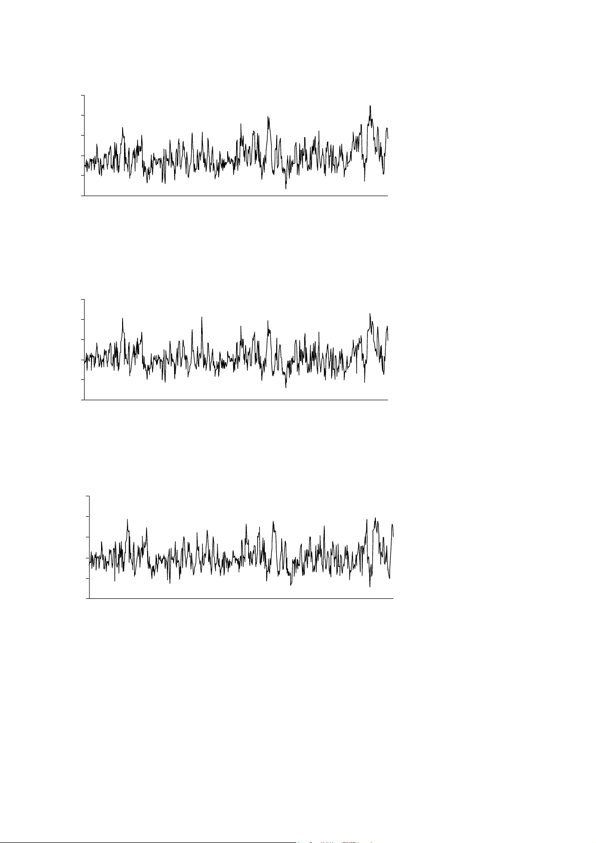
A real time model to forecast 24 hours ah ead, ozone peaks and exceedance levels. Model based on artificial neural networks, neural classifier and weather predictions. Application in an urban atmosphere in Orléans , France . Alain-Louis Dutot a, *, Joseph Rynkiewicz b , Frédy E. Steiner a , Julien Rude a a Laboratoire Inter universitaire des Systèmes Atmosphériques-UMR-CNRS-7583 Université Paris12 et Université Paris7. 61 av. du Gal. De Gaulle 94010 CRETEIL Cedex, France. b Laboratoire de Statistique Appliquée et Modélisation Stoch astique. MATISSE-SAMOS- UMR-CNRS-8595 Université Paris 1 Centre Mendès France. 90 rue de Tolbiac 75634 Paris Cedex 13, France. *Corresponding author. Laboratoire Inter univer sitaire des Systèmes At mosphériques-UMR-CNRS-7583 Université Paris12 et Université Paris7. 61 av. du Gal. De Gaulle 94010 CRETEIL Cedex, France. Tel. : 33 01 45 17 15 49 ; fax : 33 01 45 17 15 64. E-mail address : dutot@lisa.univ-paris12.fr 1 Abstract A neural network combined to a neural classi f ier is used in a re al time forecasting of hourly maximum ozone in the centre of France, in an urban atm osphere. This neural model is based on the MLP structure. The inputs of the statistical netw ork are model output statistics of the weather predictions from the French National Weather Service. These predicted meteorological parameters are very easily available thr ough an air quality network. The lead time used in this forecasting is (t + 24) hours. Efforts are related: - to a regularisation method which is based on a BIC-lik e criterion – and to the determination of a confidence interval of forecasting. W e offe r a statistical validation between various statistical models and a deterministic chem istr y-transport model. In th is experiment, with the final neural network, the ozone peaks are fa irly well predicted (in term s of global fit), with an Agreement Index = 92%, MAE = RMSE = 15 µg m -3 and MBE = 5 µg m -3 , where the European threshold of the hourly ozone is 180 µg m -3 . To improve the performance of this exceedance forecasting, instead of the previous model, we use a neural classifier with a sigm oid f unction in the output la yer. The output of the network range from [0,1] and can be in terpre ted as the probability of exceedance of the threshold. This model is compared to a cla ssical logistic regressi on. W ith this neural classifier, the Success Index of forecasting is 78 % whereas it is from 65% to 72% with the 2 classical MLPs. During the validation phase, in the Summer of 2003, 6 ozone peaks above the threshold were detected. They actually were 7. Finally, the model called NEUROZONE, is now used in real time. New data will be introduced in the training data each year, at th e end of September,. The network will be re- trained and new regression parameters estim a ted. So, one of the main difficulties in the training phase - namely the low frequency of ozone peaks above the threshold in this region - will be solved. Keywords: Artificial neural network; Mu ltilaye r Perceptron; ozone mo delling; sta tistical stepwise method; neural cl assifier; regularisation met hod; confidence interval of prediction. Software: • REGRESS : Joseph Rynkiewicz (rynkiewi@univ-paris1.fr), Laboratoir e de Statistique Appliquée et Modélis ati on Stochastique. MA TISSE-SAMOS-UMR- CNRS-8595, Université Paris 1 Centre Mendès France. 90 rue de Tolbiac 75634 Paris Cedex 13, France. http://www.samos.univ-paris.fr . Running under LINUX and SOLARIS. Free of charge. • NEUR OZON E : Alain-Louis Dutot (dutot@lisa.uni v-paris12.fr), Laboratoire Inter universitaire des Systèmes Atmosphérique s-UMR-CNRS-7583, Université Paris12 et Université Paris7. 61 av. du Gal. De Gaulle 94010 CRETEIL Cedex, France. http://www.lisa.univ-paris12.fr . Visual Basic running under Windows. Free of charge. Software required : NETRAL : www.netral.com. 3 1) Introduction According to the law, air quality agencies are commissioned to: • monitor pollutants, • forecast pollution peaks, • inform authorities and public • and assess the impact of emission reductions. For all these reasons, there is nowadays a considerab le challenge to air quality forecas ting. Tools to forecast pollution peaks can be us ed in two different ways thanks to: • 3-dimensional air quality models whic h in tegrate chemistry, tran sport and dispersion. • or statistical m odels which generally direc tly connect meteorological con ditions to level of pollutants. The first approach is time-consuming and requires v ery large databases to initializ e and run the model. Therefore, the second approach is ge nerally preferred to the first one for real time forecasting. This study focuses on photochemical smog pollution and especially on ozone pollution. Although changes in daily emissions aff ect daily ozone concentrations, it is the daily weather variations that best ex plain the day to day variability in the ozone levels (US- EPA, 1999). Ozone conducive meteorological conditions are now well-known. During the Summer, high insulation, high temperature, hi gh stability (low mixing heights), and low midday relative humidity produce photochem ical smog. The persistence of these conditions leads to ozone episodes (Alshuller and Lefohn 1996, Seinfeld and Pandis 1998, US-EPA 1996). The method presented here, consists in us ing some of these meteorological param eters - estimated from a weather forecas ting system - as the predictors of a statistic al model. 2) Method 2-1) Strategy 4 The aim of this study is to present an ozone peak forecasting method which uses, in the statistical regression f unction, easily available variables for ai r quality agencies. In this study the predicted weather data will be provided by the model output statistics of the French National Weather Service (METEO-FRANCE). Empirical ozone modelling and regression m odels in particular have been largely studied. The time series analysis can model the seasonality, the trend and the autocorrelation of the ozone variability. The regressive and autoregressive models are often used (Box and Jenkins 1976, Gonzalez-Manteiga et al 1993, Gr af-Jacottet and Jaunin 1998, Prad a-Sanchez et al 2000), but they are limited by the weakness of the modelling in the ex treme values. Regressions are a lso associated with automatic classification as in the CART method (G ardner and Dorling 2000, Ryan 1995). The possible presence of chaotic dyna mics in ozone concentrations allows the performing of non-linear time series m odelling (C hen et al 1998, Kocak et al 2000, Lee et al 1994, Raga and Le Moyne1986). Other non-linear methods such as neural networks have also been developed (Boznar et al 1993, Comrie 1997, Gardner and Dorling 1998, Ruiz-Suarez et al 1995, Yi and Prybutok, 1996, Zolgha dri et al, 2004). These neural methods provide a better representation of the extreme values than the li near ones. The use of non-linear techniques is often recommended to deal with the ozone pr ediction (Schlink et al, 2003, 2005). The aim of this paper is to test an empirical ozone m odelling using a neural network coupled with a neural classifier to improve the perfor mance of a threshold exceedance prediction. 2-2) Data set The ozone data used in this study come from LIG’ AIR - the air quality agency of the centre of France. This agency has 15 ground monito ring stations distributed over 39 540 km 2 . This region produces about 3% of the national NO x emissions and 10% of the VOC production, 38% of which come from biogenic emi ssions. In this region 85% of the NO x emissions come from mobile sources. 75% of the V OC regional emissions come from the industrial sector, 5 waste processing and agricu lture (http://www.citepa.org, http://www.ligair.fr ). This study is focused only on the city of Orléans (274 000 inhabitants) which ow ns 3 urban monitoring stations: called Préfecture (station 1), La Source (station 2) and Saint Jean de Braye (station 3). The database for developi ng the model were obtained duri ng 5 consecutive years (1999- 2003). The ozone forecasting presented here is based on the daily maxim um of the hourly mean concentrations of the background stations . As ozone peaks during the Summer, the data from April to September, are the only ones used in this model. This is the choice of the air quality network of Orléans, only to develop a “spring-summer” m odel. But, we have tested that our approach also is valid all over the year. The meteorological data used are the weather forecasts delivered by the French Weather Service ( METEO-FRANCE-département du Loiret ) for the Orléans area. These forecasts are delivered at 12 00 UTC, for the following day. The forecast bulletin (D+1), called atmogramme , contains 5 classes of predicted parameters: • the cloudiness, divided into 6 classes of weather conditions, • the rainfall, divided into 10 classes, • the surface wind speed and direction, divi ded into 6 and 8 classes respectively, • the maximum and the minimum air tem peratures, • and the vertical temperature gr adient between 0 and 300 m. The first three parameters are predicted for 3-hour intervals and th e last one for 12-hour intervals. We calculate the hourly frequency of each class of the 3 firs t types of parameters. Persistence is introduced in the analy sis by using ozone value at 12 00 UT, on D-day. These 74 meteorological variables and pers istence are used as input data in the neural network. Note that the choice of these variables is direc tly imposed by the forecast bulletin and not by a statistical or chemical criterion. But it alread y contains the main part of the relevant meteorological parameters. Unfortunately, the solar radiation is not available. But it is highly 6 correlated both to air temperat ure and cloud cover. Moreover, there are no data available on the upper-air ventilation reflecti ng the possible transport of the ozone and of the ozone precursors in and out of the site. The data used range from 1999 to 2003. Fig. 1 shows the variability of the ozone data. 2-3) Statistical model The neural model used in this study is autoregr essive and includes exoge nous parameters (it is termed a NARX model). It is based on the us e of a MultiLayer Perceptron Network. From a statistical point of view , MultiLayer Perceptrons are non -linear param etric functions. The adjustable parameters are called the weight; the exogenous variables are the inputs of the model and the estimated va riable is the output. One important f eature of MultiLay er Perceptron is its capability to model any smoot h functional relationship between one or m ore predictors and variables to be predicted. This property is c ompletely fulfilled with just one hidden layer MLP . Thus, we have employed this kind of neural network, in this study. These regressions can be presented as static singl e-output processes with an n-input vector X and an output vector Y . So, the estimated model, Y ˆ , can be represented by: ε + = ) , ( ˆ w X f Y (1) where: is the neural activation function f are the parameters of the neural reg ression to be estimated w and ε is a zero-mean random variable. Details on the use of such ne ural networks can be found, for example, in W hite (1992), Gardner and Dorling (1999), Nunnari et al (1998) and Dutot et al (2003). In this study, the hyperbolic tangent is used as the activation function, , of the neural operator. So, equation (1) is written: f ε +                 + + = ∑∑ == n i p i i i i i X w w w w Y 11 , 0 0 tanh ˆ (2) 7 The two main pitfalls in using MLP are the poo r local m inima of the error function and the overtraining of this regression function. For the first problem, a good solution is to use a sufficiently large number of rando m initializations f or the weights of the MLP to be trained. This method is time consum ing but is easy to implement in parallel . It could also be convenient to use several computers to find the best parameters. 2-3-1) Regularisation scheme Overtraining is a more complex problem. MLPs m ay be extremely overparam etrized models. It occurs when the model learns the noisy deta ils of the training data. The overtrained models have very poor performance on fr esh data. In this st udy we have used a pruning technique to avoid overtraining. This technique, both for th e parameter estim ation (in the learning process) and the model selection (in the hidden layer architecture select ion), is a stepwise method using a BIC-like criterion which has been proved consistent (Cottrell et al 1995). The MLP with the minimal dim ension is found by the elimin ation of the irrelevant weights. The m ethod essentially consists in minimizing a BIC -like info rmation criterion, tha t is to say, the mean square error of the model penalized by a f unction of the num ber of parameters and data: N N W N MSE BIC ) ln( ln + = where: • = − = ∑ 2 ) ( N 1 observed estimated X X MSE mean square error, • size of the training data = N • and W number of adjustable parameters, , of the MLP. = i w This minimization leads to the elimination of the ir relevant weights and, depending on the case, to the elimination of a few complete variab les or ev en to the elim ination of a few neural 8 units in the hidden layer. This is a way to avoid overtraining of th e learn ing phase. The determination of the final model begins with all the possible input s and with too many neurons in the hidden layer. Th en, units in the hidden layer are gradually eliminated by computing at each step the BIC-like criterion as long as its value decr eases. The calculation stops when the BIC criterion remains stable or increases. In the beginning, the first value of the weights between the inputs and the hidden layer are init ialized by the value of the parameters of a linear regression having the same inputs. The initial value of the bias is equal to the mean value of the training data. Fina lly, the elimination of these param eters, and eventually those of some inputs, leads to the m inimal MLP. One advantage of this regularisation method instead of the classical early-stopping m et hod, is to merge the learning and validation data sets into a bigger lear ning set. This methodol ogy can be found in our software REGRESS, available at http//www. samos.univ-paris1.fr, running under LINUX and SOLARIS. 2-3-2) Confidence interval of prediction Monari and Dreyfus (2002) propose to use the leverage of the examples in the training data to compute a confidence interval of the predicted va lues. Leverage is a measure of the ef fect of a particular observation on the f itted regression, due to the p osition of the observ ation in the space of the predic tor variables: i Z M T i Z ii h 1 − = where: • is the leverage of the exam ple i in the training data whic h represents the influence of in the learning phase ii h i • θ θ ∂ ∂ = ) , ( i x f i Z is the gradient of the model output w ith respect to the parameters θ • and ) ( Z T Z M = . 9 The authors show that if the m atrix Z has full rank and under asym ptotic conditions, then th e confidence interval of prediction is: ()       − − ± Z Z T Z T Z S q N t 1 α where: • is the t-distribution with q N t − α q N − degrees of freedom and a level of significance ) 1 ( α − • and       ∑ = − = N i i R q N S 1 2 1 is the residual stand ard deviation of the model. All the details of this approach can be found on http://www.neurones.espci.fr . In this work we have used a neural algo rithm of the MLP developed by NETRAL (see http://www.netral.com ). This software gives large access to the source code. The non-linear function used in the neural un its is the hyperbolic tangent. Th e optim isation method used is a second-order method: the Levenber-Marquart me thod. The cost function to be minimized according to the Delta rule is : () 2 2 1 ∑ − = estimated Y observed Y E . Classically, the initial data ar e centered and stand ardized as: X S X i X normalized i X ) ( , − = where: • is the standard deviation. X S 3) Results 3-1) Inputs selection 10 The neural network design will be obtained from the m ost representative sta tion of the urban atmosphere: station 3, Saint Jean de Bray . This choice which includes location and environmental criteria is based on the national typology and classifi cation of air quality monitoring sites. Then, the architecture (number of neurons in the hidden layer and num ber of input variables) of the network will be reproduced in the two other s tations. The database of the stations are split into 2 datasets, training and validation sets. The first dataset is used to optimise the parameters of the regression. The years 1999 to 2002 represent the training data, and 2003 the valid ation set. This valida tion dataset, which is not use d during the training phase, is u sed to assess the pe rformance of the regressio n. An ANOVA test indicated that there was not significant diffe rence between these 2 datase ts at the 95% confidence level. According to the stepwise method (REGRESS) pr esented above, the variables selection leads to keep only 8 parameters as input data: • the ozone concentration at 12 00 UTC on D-day, • the predicted (D+1) minimum and ma ximum of the air tem peratures, • the predicted (D+1) mean surface wind speed, • the predicted (D+1) hourly fr equency of wind in directi ons: S, SW, W, NW and W , • and the predicted (D+1) hourly frequency of a cloudiness class called "sky without cloud" in the atmogramme . The REGRESS method also provides the number of neuronal units in the hidden layer. Fig 2 shows that the optimum of the BI C criterion, on the validation da taset, is reached with only 1 neuron in this hidden layer. Finally, Fig 3 pres ents the diagram of the neural network. This neural structure will be us ed on the other two stations, Préfecture (1) and La Source (2) . 11 3-2) Details of model computations and model evaluation procedures The architecture of the basic neural model was shown above. We called this first model MLP 1 in the rest of the study. In Europe threshold for which an information of bad air quality in urba n areas is m ade public is the hourly mean ozone concentration: 180 µg m -3 . Looking at Table 1, it is possible to see that the observations above th e critical level of 180 µg m -3 constitute a very small part of the overall data. Only 2% of the total data exceed this thre shold. In case of such rare events, Nunnari et al (2004) propose a method of pattern balancing th at is based on artificially reducing the frequency of data with low values. Let us call and the number of episodes above and below the threshold a N b N θ . The authors propose to re-determine according to: b N a N r MLP b N ) ( * 2 , θ = with ) exp( ) ( θ θ b a r = where: • a =1 • and b =0.0125 if 0 100 < < θ . Though the European threshold is 180, we will implement this techn ique in the MLP 2 model. As seen on Table 1, in this model the number of the training data are ran domly reduced from 613 to 50 and 70 in the validation data. According to the difference in th e value of the threshold, a new balancing of the training set is proposed in this study. The size of the training set is empirically: . This model is called MLP * 2 , 2 * 3 , MLP b N MLP b N = 3 . 12 A deterministic chem istry-transport model was th en used to evaluate the other models. This model (called CHIMERE , Vautard et al, 2001) calculates, given the emissions, the meteorological variables and the lateral bounda ry conditions, the concentration fields of several pollutants, on a 6x6 km grid. The model produces th e ozone forecasts for 4 different lead times: Day + 0, Day + 1, Day + 2 and Da y + 3. The D+1 forecasts of this study will be used in comparison with the other models. De tails on the model and the experiment can be found on our Web site: http://www.lisa.univ-paris12.fr and also on: http://prevair.ineris.fr . Finally, we added the results of a multi-linea r model (called LIN ) which has the same predictors as the other models. To deal with o bvious multicollinearity of the data we have used ridge regression. Instead of parameters estim ation which is used in le ast square regression: , the ridge regression use a biased estimator: ) ( ) ( ˆ 1 Y X X X b T T i − = ) ( ) ( ~ ˆ I X X b T i + = λ 1 Y X T − , where I is the identity m atrix. The ridge param eter λ is the smallest value which gives stable estimate of i b ~ ˆ . In this study we have used 05 . 0 = λ . To evaluate the forecast system, pure persis tence m odel is included in the performance indices. It will be called : PERS . Generally, there are two main groups of perf ormance measures that can be used in the evaluation: one group represents the global fit agreement between observed and predicted data and the other represents the quality of the forecasting exceedance of a threshold value. The first group contains: • the Mean Bias Error (MBE) ∑ = − = N i i O i P N 1 ) ( 1 i P which represents the degree of correspondence between the mean forecast ( predicted data) and the m ean observation ( observed data). Values >0 indicate over-prediction. = = i O 13 • the Mean Absolute Erro r (MAE) ∑ = − N i i O i P N 1 1 = • the Root Mean Square Error (RMSE) () ∑ = − = N i i O i P N 1 2 1 0 which can be divided into systematic and unsystematic com ponents by a least square li near regression of and with slope b and intercept b . The systematic RMSE is RMSE i P i O 1 s () ∑ = − N i i O i P N 1 2 ˆ 1 = i P ˆ where is the predicted value in the linear regression: . This measure describes the linear bias produced by the model. The unsystematic RMSE , RMSE i P ˆ i O b b 1 0 + = u () ∑ = N i P 1 ˆ − = i i P N 2 1 , may be interpreted as a m easure of precision of the model. With re sp ect to a coherent model, RMSE s should approach 0 while RMSE u should approache RMSE. • the index of agreement, ( ) () ∑ = − + − ∑ = − − = N i O i O O i P N i i O i P d 1 2 1 2 1 which should approach 1 in a coherent model. • The correlation coefficient is not suitable fo r comparative study and therefore not used in this work (Willmot, 1985). In the second group of indexes all observed and predicted exceedances are classified in a contingency table. With A representing the correctly predicted exceedances, F all the predicted exceedances, M all the observed exceedances an d N the total num ber of data, we will use: • the True Positive Rate, M A TPR / = which represents the fraction of correctly predicted exceedances. It can be interpreted as the se nsitiv ity of the model. 14 • the False Alarm Rate, ( ) ( ) M N A F FAR − − = / for which ( ) FAR − 1 represents the specificity of the m odel. • and the Success Index, SI FAR TPR − = ranging from –1 to +1 w ith an optimal value of 1. Not affected by a large number of correc tly forecasted non-exceedances, SI is useful for evaluating rare events as there are in this study. Information about these performance indices can be found in Willmott et al (1985), European Environment Agency (1997) and Schlink et al (2003). Note that the diurnal maximum 1-h average oz one reference level in E urope is 180 µg m -3 (Directive 2002/3/EC). 3-3) Results of the statistical eva luation of the model performance Let us recall that the new da ta used to assess the models, come from Summer 2003 for station 3, the most representative one of the city. 3-3-1) Evaluation of the global fit agreement Table 2 shows that the index of agreement, d , of the pure persistence m odel is the weakest of all the models which are all b etter than this reference m odel. But note that the 3 MLP obtain the highest scores for this general index (92%). Among these 3 m odels, MLP 1 is the most accurate (as RMSE unsystematic = 12 µg m -3 and MAE = 15 µg m -3 ). They are 17, 16, 26 µg m -3 and 18, 17, 24 µg m -3 for MLP 2 , MLP 3 and CHIMERE respectively. Once again, the Mean Bias Error is lower, for MLP 1 . Note that the 3 MLP models are slightly over-estim ated (respectively: 5, 11 and 7 µg m -3 ) whereas the deterministic m odel has a bias of –13 µg m -3 . The authors of this model explain the negati ve bias could be due to a problem in the representation of anthropic and biogenic emissions of V OCs during summer 2003. This problem now is solved. Finally, regarding th ese fit indices, we can select the MLP 1 model as 15 an efficient forecasting system. Fi g. 4 summarizes the resu lts of Day+1 forecasts at station 3 during the validation period for both the MLP 1 and the deterministic models. 3-3-2) Evaluation of the exceedance indexes The essential quality of a forecast model is its ab ility to correctly predic t concentrations above the threshold. The success index (SI) can m easure this ability. To evalu ate the perform ance of the exceedance forecasting, we have calculated th e frequency of the predictions such as: a correct prediction is retained if 180 1 ≥         −       − + Z Z T Z T Z S q N t estimated α C where ()       − − Z Z T Z T Z S q N 1 α t is the confidence interval c alcul ated as shown in paragraph 2-3. For MLPs models, the best Success I ndex (72%) is obtain ed with the MLP 3 which uses our pattern balancing [see table 2]. But, this model also has one of the higher False Alarm Rate, 14%. This sensitivity gives 12 false alarms on the validation period while the observed exceedances only are 7. The model associated with the lowest FAR (6%) is the MLP 1 but this model also has about the same SI (65%) than the pure persistence model ! So, it is clearly difficult to do the right choice. 3-3-3) Development of a neural classi fier to perform the exceedance levels According to the difficulties to choose the right model of ex ceedance, we want to present in this work a significant improvement of the sc ores by using a new neural model. As seen above, the MLP 1 model is the best in terms of global f it. W ith the same neural structure, we have built a new neural network wi th a sigmoid neural function in the output layer instead of the identity f unction. The MLP network was def ined as: . ∑ = ∑ = + + =             n i p i i X i w i w i w w MLP Y 11 , 0 tanh 0 1 ˆ 16 The new neural network, which is called classifier , will be:         ∑ =                   ∑ = + + + = n i p i i X i w i w i w w classifier Y 11 , 0 tanh exp 1 1 0 ˆ . All the input data are now ranging from [ ] 1 , 0 . The output of the network in the training data is no longer the ozone peak but with: i p • if 0 = i p 180 1 <         −       − + Z Z T Z T Z S q N t estimated C α • if 1 = i p 180 1 ≥         −       − + Z Z T Z T Z S q N t estimated C α If: • is the number of tra ining data in the class A N 1 = i p • is the probability dens ity function of the class A () x f A • is the number of tra ining data in the class B N 0 = i p • is the probability dens ity function of the class B () x f B then the function ( ) () () x f N x f N x f N x A P B B A A A A + = is the a posteriori class-condition al density function of A given x . Because of the sigmoid function in the output layer, th e output o the classifier in the validation set, Y , is also ranging from i , classifier ˆ [ ] 1 , 0 . It can be interpreted as the probability of exceedance of the threshold 180 µg m -3 . This classifier is used on the same training data, with the same predictors and evaluated on the sam e validation set. If Y , we admit a 50 . 0 i , classifier ˆ ≥ 17 prediction of exceedance. Table 2 shows that the SI of the classifier is the highest (78%) associated with one of the lowest FAR (8%). Using the best MLP model (MLP 3 ) these scores with a 95% confidence int erval are 72% and 14% respectively. Fig. 5 s hows the probability of exceedance during the validation phase. 6 ozone peaks have been detected above 180 µg m -3 on 7 real alarms. And there are 6 false predic tions. The correctly p redicted exceedances for MLP 3 were only 4 out of 7. This method clear ly shows a significant improvem ent in the prediction of the peak con centrations above 180 µg m -3 . Is this method more accurate than a classical logistic regression ? A logistic model fits a response of observed proportions o r probabilities at each level of an independent variable. The logistic model is defined by the equation: ∑ ∑ + + + = i i i i i i x b a x b a y ) exp( 1 ) exp( The response function of this model is a non-lin ear S-shaped curve with asymptotes at 0 and 1. In this study, after rem oving the no significant variables by using a stepwise technique, the best logistic model with the same data only uses 3 exogenous variables: • the ozone concentration at 12 00 UTC on D-day, • the predicted mean surface wind speed, • and the predicted hourly frequenc y of wind in direction: SW. And the equation of th e logistic model is: ) day ozoneonD 091 . 0 windspeed 4092 . 0 SW 8074 . 0 23 . 12 exp( 1 ) day ozoneonD 091 . 0 windspeed 4092 . 0 SW 8074 . 0 23 . 12 exp( exceedance of y probabilit − + − − − + − + − − − = The p-value of the model and the residual are 0.0001 and 1.00 respectively. Because the p- value of the model is less than 5%, there is a statistically sig nificant relationship between the variables at the 95% or higher confidence level. In addition, the p-value of the residuals 18 indicates that the m odel is not significantly wo rse than the best possible model for this data set at the 95% confidence interval. The Chi-s quare goodness of fit test p-value is 0.76. This determines whether the logistic function adequately fits the obs erved data. In this study there is no reason to reject the adequ acy of the fitted model at the 95% or higher confidence level. The results of this logistic re gression during the validation pha se are shown on Fig. 5. This figure shows that all the observed exceedances ar e correctly predicted . Especially the last isolated peak in the end of September, not seen by the classifier model, is correctly forecasted with the logistic model. Unfortunately the Fig. 5 also shows that th is method is too mu ch sensitive. There are 29 false alarms during th is validation period. So, the Success Index of the logistic model becomes worse than those of th e classifier: 66% and 78% respectively [see table 2]. Finally, the neural classifier remains the be s t candidate for the exceedance forecasting. 3-3-4) Forecasting on the other two stations The same neuronal structure (MLP 1 ), that is to say, the same predictors and the sam e hidden layer, is applied to the data of stations 1 a nd 2. A new training is m ade for each station with the data of 1999-2002 and a validation phase is ma de with the data of the year 2003. Fig.6 shows all the results f or the 3 stations. The slopes of the linear regression of this scatter plot are 0.70 0.15, 0.72 ± ± 0.12 and 0.70 ± 0.15 for station 1, 2 and 3 respectively. Let us remember that station 3 was used as reference. It is easy to see that there is no significant difference between these values. The anal ysis of the standardized residual, SR, ( S observed C C SR − = estimated where is the standard deviation of the observed data) indicates that the variation of these values is less than S S 2 ± , and that no special pattern appears in the 19 residuals, Fig. 7. Therefore, these 3 models can be globally validated to evaluated the global fit agreement. The neural classifier applied to the data of st ations 1 and 2 gives the results shown on Table 3. All the observed exceedances are correctly for ecasted for station 1. The SI has the higher score (89%). For the station 2, 6 exceedances out of 8 have been found. The SI is 70% for this station. 4) Conclusion We have presented the results of an hourly ma ximum ozone forecast in an urban atmosphere. The system is based on an artificial neural network for which the input data come from meteorological model output stat istics. Meteorological forecasts 24 hours ahead used in this model are easily available data provided by any National Weather Service. In this study, our aim was essentially to find these exogenous parame ters and, of course, to develop an easily operational ozone system forecasting. The validation procedure consists in com par ing the forecasts with observations over a complete Summer season, from April to September 2003. One Multilayer Perceptron and two MLPs with a pattern balancing are tested. In comparison, w e use a deterministic m odel and the persistence m odel as references. For the global fit agreement, the MLP network without balanci ng shows the best scores of prediction 24 hours ahead with and the best precisi on of the model with and % 92 = d 3 m µg 15 − = MAE 3 m µg 12 − = ic unsystemat RMSE . For the ability to predict the exceedance of the Eur opean threshold (180 µ g m -3 ), the MLP with our balancing of the trai ning data has the best Success I ndex (72%) but the False Alarm Rate is the higher (14%). According to the di fficulty to choose the right model for exceedance forecasting, we have developed a neural classifier. The output of this m odel ranges from 0 to 20 1 and can be interpreted as the probability of the exceedance of the 180 threshold. Using this classifier during the validation phase, 6 exceedances out of 7 have been found. The Success Index reaches 78% and the False Alarm Rate only is 8%. This is the best com bined performance of all the models. Our model, now called NEUROZONE , has been implemented in real-tim e in the Orléans region. Each year, at the end of September, the validation data will be introduced into the former training data. Year af ter year, the network will be re-trained and new regress ion parameters estimated. So, one of the main difficulties in the tra ining phase - namely the low frequency of ozone peaks above th e threshold in this region - will be solved. In this study we have focused on a 24 hours ahead forecasting. In the future, it would be possible to introduce forecasting with longer lead times. Acknowledgements This forecasting project was supported by th e air quality network of the Orléans region ( LIG'AIR ).We are also grateful to the Fren ch National Meteor ological network ( METEO- FRANCE ) for the weather forecasts. INERIS graciously supplied us with the m odel- predicted data of the CHIMERE-PREV'AIR 2003 experiment, we gratefully acknowledge their assistance. 21 References Altshuller A. P., Lefhon A.S., 1996. Backgr ound ozone in the planetary boundary layer over the United States. Journal of Air & Wast e Management Association, 76, 137-171. Box G.E., Jenkins G.M., 1976. Time series analysis. Forecasting and control. Holden Day, San Francisco. Boznar M., Lesjak M., Mlakar P., 1993. A ne ural network-based method for short-term predictions of ambient SO 2 concentrations in highly pollu ted industrial ar eas of complex terrain. Atmospheric Environment, 27B, 2, 211-230. Chen J.L., Islam S., Biswas P., 1998. Nonlin ear dynamics of hourly ozone concentrations: nonparametric short-term prediction. At mospheric Environment, 32, 1839-1848. Comrie A.C., 1997. Comparing neural networks and regression m odels for ozone forecasting. Air & Waste Management Association, 47, 653-663. Cottrell M., Girard B., Girard Y., Mangeas M. , Muller C., 1995. Neural modelling for tim es series. a statistical stepwise method for weight elimination. Neural Networks, 6, 1355- 1364. Directive 2002/3/EC: of the European Parliament and of the Council of 12 February 2002, relating to ozone in ambient air, see:http://europa.eu.int/eur- lex/pri/en/oj/dat/2002/1_067/1_06720020309env00140030.pdf. Dutot A.L., Rude J., Aumont B ., 2003. Neural network method to estimate the aqueous rate constants for the OH reactions with organi c compounds. Atmospheric Environment, 37, 269-276. European Environment Agency, 1997. National Ozone Forecasting Systems and International Data Exchange in Northwest Europe. Techni cal Report 9. R.M. van Aalst and F.A.A.M. de Leeuw Ed.. 22 Gardner M.W., Dorling SR., 1998. Artificial ne ural networks, the multilayer Perceptron. A reiew of applications in the atmospheric sc iences. Atmospheric Environment, 32, 14/15, 2627-2636. Gardner M.W., Dorling SR., 1999. Neural ne twork m odelling and prediction of hourly NO x and NO 2 concentrations in urban air in London. Atmospheric Environment, 33, 709-719. Garner M.W., Dorling S.R., 2000. Statisti cal surface ozone m odels: an improved methodology to account for non-linear behaviour. Atmospheric Environm ent, 34, 21-34. Gonzalez-Manteiga W., Prada-Sanchez J.M., Ca o R., Garcia-Ju rado I., Febrero-Bande M., Lucas-Domingez T., 1993. Time series analys is for ambient concentrations. Atmospheric Environment, 27A, 2, 153-158. Graf-Jacottet M., Jaunon M-H., 1998. Predictiv e models for ground ozone and nitrogen dioxide time series. Envi ronmetrics, 9, 393-406. Kocak K., Saylan L., Sen O., 2000. Nonlinear time series prediction of oz one concentration in Istanbul. Atmospheric Environment, 34, 1267-1271. Lee I.F., Biswas P., Islam S., 1994. Estimation of the dominant degree s of freedom for air pollutant concentration data: ap plicati on to ozone measurement. Atm ospheric Environment, 28, 1707-1714. Monari G., Dreyfus G., 2002. Local overfitting control via leverage s. Neural Computation, 6, 1481-1506. Nunnari G., Nucifora A., Randi eric C., 1998. The application of neural technics to the modelling of times series of atmospheric pollution data. E cologica l Modelling, 11, 187- 205. Nunnari G., Dorling S., Schlink U., Cawley G., Foxall R., Chatte rton T., 2004. Modelling SO2 concentration at a point with statisti cal approaches. Environmental Modelling & Software, article in press, corrected proof. 23 Prada-Sanchez J.M. Febrero-Bande M., Cotos-Y anez T., Gonzalez-Manteiga W., Berm udez- Cela L., Lucas-Domingez T., 2000. Prediction of SO2 pollution inci dent near a power station using partially lin ear models and an historical m atr ix of predictor-response vectors. Environmetrics, 30, 3987-3993. Ruiz-Suarez J.C., Mayora-Ibarra O.A., Torres-Ji menez J., Ruiz-Suarez L.G., 1995. Short-term ozone forecasting by artificial neural network. Advances in Engineering Sotware, 23, 143- 149. Ryan W.F., 1995. Forecasting ozone episo des in the Baltimore metropolitan area. Atmospheric Environment, 29, 17, 2387-2398. Seinfeld J.H., Pandis S.N., 1998. Atmospheric chemistry and physics. from air pollution to global change. J. Wiley, New York. Schlink U., Dorling S., Pelikan E., Nunnari G ., Cawley G., Junninen H., Greig A.., Foxall R., Ebeb K., Chatterton. T., Vondr acek J., Richter M., Dostal M., Bertucco L., Kolehm ainen M., Doyle M., 2003. A rigourous inter-compar ison of ground-level ozone prediction s. Atmospheric Environment, 37, 3237-3253. Schlink U., Herbarth O., Richter M., Dorling S ., Nunnari G., Cawley G., Pelikan E., 2005. Statistical models to asse ss the health effects and to forecast g round-level ozone. Environmental Modelling & Sof tware, in Press. Us Environmental Protection Agency, 1996. Air qua lity data. Ozone and precursors, chap. 1. Office of Air Quality Planni ng and Standards, Research Triangle Park, North Carolina 27711. Us Environmental Protection Agency, 1999. Gu ide lin e for developing an ozone forecasting program. Office of Air Quality Planning and S tandards, Research Triangle Park, North Carolina 27711. 24 Vautard R., Beekmann M., Roux J., Gom bert D., 2001. Validation of a hybrid forecasting system for the ozone concentration s over th e P aris area. Atmosphe ric Environment, 35, 2449-2461. White H., 1992. Artificial neural ne tworks. Blackwell Ed., New York. Willmott C.J., Ackleson S.G., Davis R.E., Fedde m a J.J., Klink K.M., Legates D.R., O'Donnell J., Rowe C., 1985. Statistics for the eval uation and comparison of m odels. J. of Geophysical Research, 90, C5, 8995-9005. Yi J., Prybutok V.R., 1996. A neural network model forecasting for pred iction of daily maximum ozone concentration in an industria lized urban area. Environmental Pollution, 92, 3, 349-357. Zolghadri A., Monsion M., Henry D., Marchionini C., Petrique O., 2004. Developm ent of an operational model-based warning system fo r tropospheric ozone concentrations in Bordeaux, France. Environmental Modelli ng & S oftware, vol. 19, issue 4, 369-382. 25 Figures and Tables captions Fig. 1 Hourly maximum ozone from 1999 to 2003, during the Summ er period - April to September. Fig 2 BIC-like criterion according to the num ber of neurons in the hidden layer of the validation set. Note that the MLP with 0 neuron is a m ultilinear regression. Fig. 3 Structure of the artificial n eural network after the opti m ization by REGRESS. Fig 4 Time series of the MLP 1 (in red) and the determ inistic models (in green) [a] during the validation phase. [b] zooming on August 2003. Fig 5 Probability of exceedance of the Europ ean threshold, during the validation phase (April to September 2003). Observations are in black, fo recasted probability of the classifier are red squares and forecasted probability of the logistic model are blue squares. Fig 6 Scatter plot of the measured and for ecasted maxim um ozone concentrations at the 3 ground-stations. Fig 7 Standardized residual analysis on the validation dataset. Table 1 Composition of the training and validati on sets; in brackets the number of value >180 µg m -3 , outside the total number of data. Table 2 Performance measures of all the m odels during the valida tion phase: April to September 2003. Table 3 Performance measures of the exceedance forecasting for the 3 stations. 26 St at ion 1 Préfect ure 0 50 100 150 200 250 1 36 71 106 141 176 211 246 281 316 351 386 421 456 491 526 561 596 631 666 Days from 1999 t o 2003 Ozone µg/m3 St ation 2 La Source 0 50 100 150 200 250 1 36 71 106 141 176 211 246 281 316 351 386 421 456 491 526 561 596 631 666 Days from 1999 t o 2003 Ozone µg/m3 St at ion 3 Sai nt Jean de B r ay 0 50 100 150 200 250 1 36 71 106 141 176 211 246 281 316 351 386 421 456 491 526 561 596 631 666 Days from 1999 t o 2003 Ozone µg/m3 Fig. 1 Hourly maximum ozone from 1999 to 2003, during the Summer period - April to September. 27 -1 ,4 -1 ,2 -1 -0 ,8 -0 ,6 -0 ,4 -0 ,2 0 0123456789 num ber of neur ons in t he hidden l ayer BIC-like criterion Fig 2 BIC-like criterion according to the num ber of neurons in the hidden layer in the validation phase. Note that the MLP with 0 neuron is a multi -linear regression. 28 ozone concentration D-day D+1-day max, min Temperature D+1-day wind speed D+1-day wind direction D+1-day cloud cover Bias Hourly maximum ozone f=tanh Fig. 3 Structure of the artificial neural network after the optimization by R EGRESS. 29 (a ) 0 50 100 150 200 250 300 1 9 17 25 33 41 49 57 65 73 81 89 97 105 113 121 129 Days fr om A pr i l t o S ept em ber 2003 Ozone µg/m3 deter m i ni sti c m odel Ob s e r va t i o n MLP 1 Eur op ean thr eshold (b ) 0 50 100 150 200 250 300 1 4 7 10 13 16 19 22 25 28 31 34 37 40 43 Ozone µg/m3 Fig 4 Time series of the MLP 1 (in red) and the determ inistic models (in green) [a] during the validation phase. [b] zooming on August 2003. 30 0 0, 1 0, 2 0, 3 0, 4 0, 5 0, 6 0, 7 0, 8 0, 9 1 1 4 7 1 0 1 31 6 1 9 2 22 52 8 3 13 43 7 4 04 34 6 4 95 25 5 5 86 1 6 46 77 0 7 37 67 9 8 28 58 8 da ys from A pri l to Se ptembe r pr ob . o f ex ceedan c e obs er v at i on f o r e ca st( cla ssif ie r ) f o r e ca st( lo g istic) Fig 5 Probability of exceedance of the Europ ean threshold, during the validation phase (April to September 2003). Observations are in black, fo recasted probability of the classifier are red squares and forecasted probability of the logistic model are blue squares. 31 0 50 100 150 200 250 300 0 50 100 150 200 250 300 obser ved oz one µ g/ m 3 estimated ozone µg/m3 stat i on1 stat i on2 stat i on3 Fig 6 Scatter plot of the measured and for ecasted maxim um ozone concentrations at the 3 ground-stations. 32 -3 -2 -1 0 1 2 3 observation µg/m3 standardized residual station1 station2 station3 Fig 7 Standardized residual analysis on the validation dataset. 33 MLP 1 MLP 2 MLP 3 1999 tra ining 159(1) 10(1 ) 20(1) 2000 tra ining 161(0) 0( 0) 0(0) 2001 tra ining 162(3) 30(3 ) 60(3) 2002 tra ining 131(1) 10(1 ) 20(1) total training 613(5) 50(5 ) 100(5) 2003 valid ation 105(7) 70(7 ) 105(7) Table 1. Composition of the training and valid ation sets; in brackets the n umber of value >180 µg m -3 , outside the total number of data. 34 MBE MAE RMSE RMSE s RMSE u d FAR SI PERS -2 20 20 8 19 0,88 0.07 0,64 LIN 5 17 14 14 11 0,90 0.02 0.12 MLP 1 5 15 15 11 12 0,92 0.06 0.65 MLP 2 11 18 18 12 17 0,92 0.17 0.69 MLP 3 7 17 18 8 16 0,92 0.14 0. 72 CHIMERE -13 24 30 14 26 0,89 0.05 0. 52 Classifier - - - - - - 0.08 0.78 Logisti c - - - - - - 0.34 0.66 Table 2 Performance measures of all the m odels during the valida tion phase: April to September 2003. 35 36 Station 1 Station 2 Station 3 (reference) FAR 11% 5% 8% SI 89% 70% 78% Observed peak 6 8 7 Forecasted peak 6 6 6 False alarm 10 4 6 Table 3 Performance measures of the exceedance forecasting for the 3 stations.