Color Graphs: An Efficient Model For Two-Dimensional Cellular Automata Linear Rules

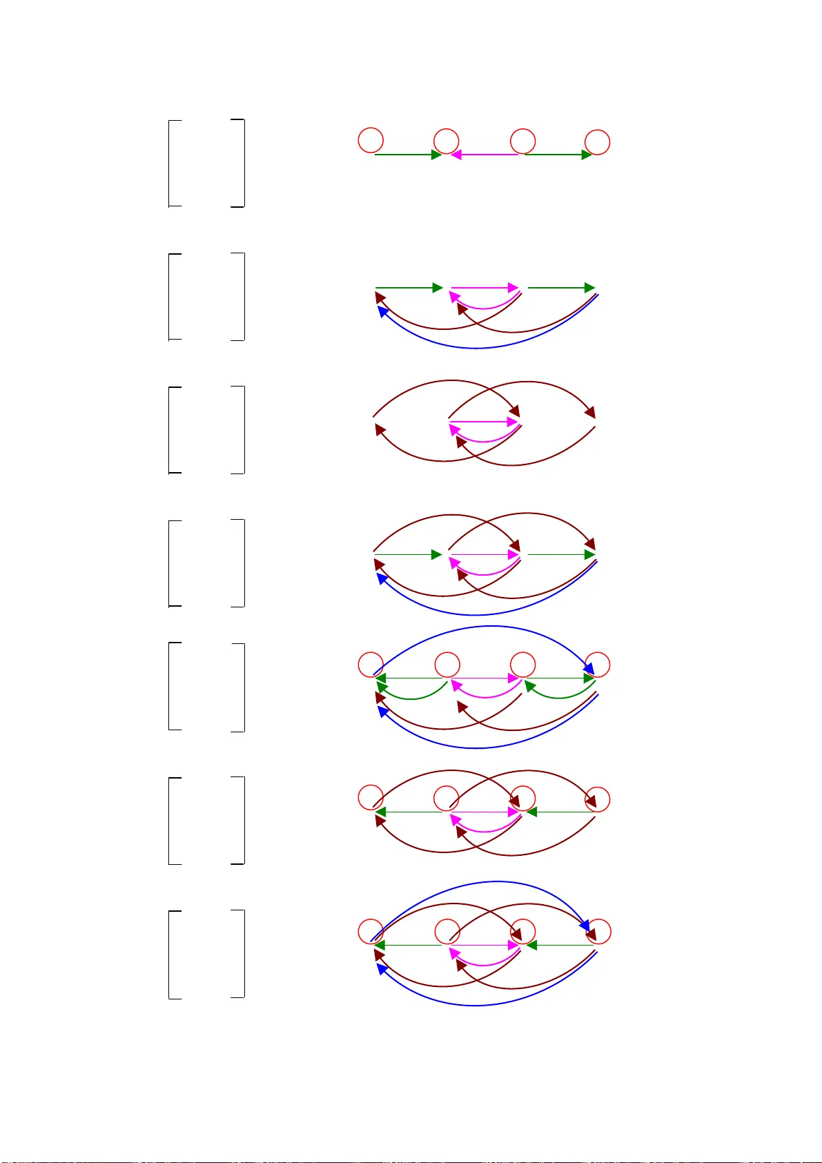
Color Graphs: An Efficient Model For Two-Dimensional Cellular Automata Linear Rules 1 BIRENDRA KUMAR NAYAK, 2 SUDHAKAR SAHOO 3 SUSHANT KUMAR ROUT 1 P.G.Department of Mathematics, Utkal University, Bhubaneswar-751004 bknatuu@yahoo.co.uk 2 Department of CSEA, SIT, Silicon Hills, Patia, Bhubaneswar-751024 sudhakar.sahoo@gmail.com 3 Department of M athematics, Raya gada College, Rayagada, Orissa Abstract: - . Two-dimensional nine neighbor hood rectangular Cellular Autom ata rules can be modeled using many different techniques like Rule matrices, State Transition Diagrams, Boolean functions, Algebraic Norm al Form etc. In this paper, a new model is introduced usi ng color graphs to model all the 512 linear rules. The graph theoretic properties therefore studied in this paper simplif ies the analysis of all linear rules in comparison with other ways of its study. Keywords: - Cellular Automata, Boolean functions, Graphs, Linear rules, Adjacency matrix. 1 Introduction Originally John Von Neumann [3] introduced Cellula r Automata (CA). A CA is a processing algorithm applied to a matrix of a fixed dimension with resp ect to space of locally connected cells whose mutual interactions determine their behaviors: time and space are discretized into intervals and cells, respectively. In forties mathematician Stanislas Ulam was interested in the evolution of graphics constructions generated by simple rules. The base of his constructions was a two-dime nsional space divided into “cells”, a sort of grid. Each of these cells could have two states: ON or OFF. St arting from a given pattern, the following generation was determined according to neighborhood rules. For example, if a cell was in contact with two “ON” cells, it would switch on to ON states; otherwise it would switch off. Ulam, who used one of the first computers, quickly noticed that this mechanism perm itted to generate complex a nd graceful figures and that these figures could, in som e cases, self-reproduce. Extremely simple rules pe rmitted to build very com plex patterns. In this paper a 2-dimensional Cellular Automata is considered and each cell is influenced by its 9-neighboring cells including itself. The cells are characterized by its ce ll states; here we are considering the states are either 0 or 1. A 2-dimensional grid can be divided into several cells possessing states in binary. These binary data gives a binary information matrix (also referred as binary problem m atrix or binary image) whose order is equal to the size of the grid say (m x n). Then, the rules of influen ces of each cell by its neighboring cells can be obtained by applying the rule to this binary information matrix, ge tting another binary information matrix, which gives the information about its next generation. These influences can be captured through matrices [1, 8, 9] , which we call as rule matrices. The binary information matrix of order (m x n) is reduced to a co lumn m atrix of order (mn x 1), arranged in a row major order, such that a (mn x mn) rule ma trix must be necessary for applying it to this binary information matrix arranged in one-dimension. To study the properties of these rule m atrices of 0’s and 1’s even for a small value of m and n are quite difficult. Although some interesting patte rn and characteristics of these matrices has reported in [9] still there is a necessity to get a better handle to get some more information of these rules. In this paper, rule matrices are characterized by color graphs, which dete rmine several interesting characteristics of rules. In chapter 2, a review of earlier works in Cellu lar Automata and some ideas, which will be needed in our work, has been made. Here, we undertake the study of 2-dimesional CA where in each cell is assumed to be influenced by its 9 neighbors. The rules of influence are captured by the matrix representations of the linear Boolean functions with 9-variables. In chapter-3, we ha ve studied the problems of 512 linear Boolean rules with 1 9-variables and the matrix representing them. In chapter-4 , an attempt is being made to understand the graphical representation of rule matrices. 2 Review of Earlier w ork on 2-D CA In 2-D Nine Neighborhood CA the next state of a particular cell is affected by the current state of itself and eight cells in its nearest neighborhood. Such dependenc ies are accounted by various rules. For the sake of simplicity, in this section we take into consideration only th e linear rules, i.e. the rules, which can be realized by EX-OR operation only. We want to find some algebraic properties of these 2 9 =512 linear CA rules that are quite useful to describe the behavior of 2-D Cellular Automata and its enumerable number of application reported in [2, 3, 6]. A specific rule convention that is adopted to num ber all 512 rules reported in [8, 9] is as follows: 64 128 256 32 1 2 16 8 4 Fig-1 The central box represents the current cell (i.e. the ce ll being considered) and all other boxes represent the eight nearest neighbors of that cell. The number within each box represents the rule number characterizing the dependency of the current cell on that par ticular neighbor only. Rule 1 characterizes dependency of the central cell on itself alone whereas such dependency only on its top neighbor is characterized by rule 128, and so on. These nine rules are called funda mental rules. In case the cell has dependency on two or more neighboring cells, the rule number will be the arith m etic sum of the numbers of the relevant cells. For example, the 2D CA rule 171 (128+32+8+2+1) refers to the five-neighborhood dependency of the central cell on (top, left, bottom, right and itself). The number of such rules is 9 C 0 + 9 C 1 + . . . + 9 C 9 =512 which includes rule characterizing no dependency. The application of linear rules mentioned in the pr evious section can be realized on a problem matrix, where every entry is either 0 or 1. Illustration In figure 2, Rule 170 (2 + 8 + 32 + 128) is applied uniformly to each cell of a problem ma trix of order (3 x 4) with null boundary condition (extreme cells are connected with logic-0 states). 170 00 1 0 1011 11 1 0 0010 10 1 1 1101 Rule ⎛⎞ ⎛ ⎜⎟ ⎜ ⎯⎯ ⎯ ⎯ → ⎜⎟ ⎜ ⎜⎟ ⎜ ⎝⎠ ⎝ ⎞ ⎟ ⎟ ⎟ ⎠ [Fig-2: shows the cell under consideration, will change its state by adding the states of its 4 orthogonal neighboring cells. 0+1+1+1=1. Similarly, Rule 170 is applied to all other cells.] Also for this problem matrix of dim ension (3 x 4) , Rule 170 using an algorithm reported in [9, 10] can be realized as another binary matrix of dimension (12 x 12) called rule matrix for rule 170 which when m ultiplied with a (12 x 1) column vector (in this case [0 0 1 0 1 1 1 0 1 0 1 1] T ) formed from the problem matrix in a row major order gives the same output im age. 2 3 Graph representation of Basic linear rules As rule matrices are basically binary square matrices of dimension (mn x m n) for a binary information matrix (m x n) , therefore these matrices can be realized as adjacency matrices that give a graph with vertices and edges. As every adjacency matrix is a vertex-vertex relationship so each row (or column) of the Rule m atrix corresponds to a vertex of the graph, which also refers to as each ce ll of the binary information matrix. The position of 1’s present in each row in the Rule matrix represents the nine-neighbor hood dependency of the cell for that row. So for a particular (m x n) binary image one can constr uct 512 different graphs for 512 rules. All these graphs contain mn number of vertices num bered as v 1, v 2, … v mn where vertex v i corresponds to i th cell counting starting from the left most corner (0, 0) position of (m x n) pr oblem matrix in a row major order and the edges between the vertices denotes their nine-neighborhood dependency fo r their corresponding cell positions in the problem matrix. There are five fundamental rules Rule1, Rule2, Ru le4, Rule 8 and Rule 16 shown in Fig-1 are known as basic rules also discussed in [10] as other fundam ental rul es Rule32, Rule64, Rule128 and Rule 256 can be obtained from these with a transpose operation. The graphical re presentation of these 5 basic rules and other fundamental rules are explained through some theorems as follows: Theorem 3.1: For an m x n problem m atrix, the rule graph for Rule 1(i.e. G 1 ) has mn self loops. Example 3.1 Let us consider a 2 x 3 problem matrix, it’s rule m atrix is of order (6 x 6) (i.e. M 6x6 ) For Rule 1 (i.e. M 1 ), the matrix form is 1 1 00000 0 1 0000 00 1 000 000 1 00 0000 1 0 00000 1 M ⎛⎞ ⎜⎟ ⎜⎟ ⎜⎟ = ⎜⎟ ⎜⎟ ⎜⎟ ⎜⎟ ⎜⎟ ⎝⎠ It’s graphical form is • • • • • • V 1 V 2 V 3 V 4 V 5 V 6 [The graph has 6 independent loops] Theorem 3.2: For an m x n problem matrix, the rule matrix for Rule 2 (i.e. M 2 ) has m components and each component has n-vertices. Therefore vertex V i of Rule 2 graph connects with vertex V i+1 except i = kn, n ∈ N. Example 3.2 Let us consider a 2x3 problem matrix, it’s rule m atrix is of order 6 x 6(i.e. M 6x6 ). For Rule 2(i.e. M 2 ), the matrix form is 3 2 0 1 0000 00 1 000 000000 0000 1 0 00000 1 000000 M ⎛⎞ ⎜⎟ ⎜⎟ ⎜⎟ = ⎜⎟ ⎜⎟ ⎜⎟ ⎜⎟ ⎜⎟ ⎝⎠ It’s graphical form is V 1 V 2 V 3 V 4 V 5 V 6 [The graph has two components and each com ponent has 3 vertices] Theorem 3.3: For an (m x n) problem m atrix, the vertex V i of Rule 4 graph connects with vertex V n+i+1 for i=1,2,…mn - n-1 except i = n and mn – (n-1) i.e. V n and V mn- n+ 1 are two isolated vertices. Example 3.3 Let us consider a 3x4 problem matrix, it’s rule m atrix is of order 12 x 12(i.e. M 12x12 ). For Rule 4(i.e. M 4 ), the matrix form is 4 000000000000 000000000000 00000 1 0 00000 000000 1 00000 0000000 1 0000 000000000000 000000000 1 00 0000000000 1 0 00000000000 1 000000000000 000000000000 000000000000 M ⎛⎞ ⎜⎟ ⎜⎟ ⎜⎟ ⎜⎟ ⎜⎟ ⎜⎟ ⎜⎟ ⎜⎟ = ⎜⎟ ⎜⎟ ⎜⎟ ⎜⎟ ⎜⎟ ⎜⎟ ⎜⎟ ⎜⎟ ⎜⎟ ⎜⎟ ⎝⎠ It’s graphical form is • • • • • • • • • • • • V 1 V 2 V 3 V 4 V 5 V 6 V 7 V 8 V 9 V 10 V 11 V 12 Here V 5 and V 9 are isolated vertices. 4 Theorem 3.4: For an m x n problem ma trix, the vertex V i of Rule 8 graph connects to vertex V n+i , that is the edges are (V i,, V n+i ) for i=1,2,…,n. Example 3.4 Let us consider a 2x4 problem matrix, its rule matrix is of order 8 x 8(i.e. M 8x8 ). For Rule 8(i.e. M 8 ), the matrix form is 8 0000 1 000 00000 1 00 000000 1 0 0000000 1 00000000 00000000 00000000 00000000 M ⎛⎞ ⎜⎟ ⎜⎟ ⎜⎟ ⎜⎟ ⎜⎟ = ⎜⎟ ⎜⎟ ⎜⎟ ⎜⎟ ⎜⎟ ⎜⎟ ⎝⎠ It’s graphical form is • • • • • • • • V 1 V 2 V 3 V 4 V 5 V 6 V 7 V 8 Theorem 3.5: For an m x n problem matrix, the vertices V 1 and V mn of Rule 16 graph are isolated, other pair of vertices are joined in the sequence (V i, , V n+i-1 ) for i=2 to (mn-2). Example 3.5 Let us consider a 2 x 3 problem matrix, it’s rule matrix is of order 6 x 6 (i.e. M 6x6 ). For Rule 16(i.e. M 16 ), the matrix form is 16 000000 000 1 00 0000 1 0 000000 000000 000000 M ⎛⎞ ⎜⎟ ⎜⎟ ⎜⎟ = ⎜⎟ ⎜⎟ ⎜⎟ ⎜⎟ ⎜⎟ ⎝⎠ Its graphical form is • • • • • • V 1 V 2 V 3 V 4 V 5 V 6 Here V 1 and V 6 are isolated vertices. 5 Theorem 3.6: The graph for Rule 32, Rule 64, Rule 128 and Rule 256 are same as Rule 2, Rule 4, Rule 8 and Rule16 respectively with opposite direc tion as corresponding matrices are transpose to each other reported in [9]. Example 3.6 Let us consider a (2 x 3) problem matrix, the rule matrix is of order (6 x 6) 2 0 1 0000 00 1 000 000000 0000 1 0 00000 1 000000 M ⎛⎞ ⎜⎟ ⎜⎟ ⎜⎟ = ⎜⎟ ⎜⎟ ⎜⎟ ⎜⎟ ⎜⎟ ⎝⎠ 32 2 000000 1 00000 0 1 0000 000000 000 1 00 0000 1 0 T M M ⎛⎞ ⎜⎟ ⎜⎟ ⎜⎟ == ⎜⎟ ⎜⎟ ⎜⎟ ⎜⎟ ⎜⎟ ⎝⎠ Rule 2 graph V 1 V 2 V 3 V 4 V 5 V 6 Rule 32 graph V 1 V 2 V 3 V 4 V 5 V 6 4 Construction of graphs of all linear rules from the basic graphs In this section a new operation called join operation ca lled Join operation is introduced which is used to combine some or all of the basic graphs to form a new graph. Definition 4.1: If there is edge between two vertices, it is consid ered as 1 and if there is no edge between two vertices, then it is considered as 0. The join operation is defined as follows 0 + 0 = 0 1 + 0 = 1 0 + 1 = 1 1 + 1 = 0 When two edges between two vertices are joined the result is no edge between them. 6 Example 4.1 • • • • V 1 V 2 V 1 V 2 G 1 G 2 • • (There exist no edge between V 1 & V 2 ) G 1 + G 2 ⇒ V 1 V 2 Example 4.2 • • • • • • V 1 V 2 V 3 V 1 V 2 V 3 G 1 G 2 G 1 + G 2 ⇒ • • • V 1 V 2 V 3 Example 4.3 Consider a (2 x 2) problem ma trix. Its Rule Matrix is of order (4 x 4) The graph of Rule 1 that is G 1 corresponding to matrix M 1 is as follows • • • • V 1 V 2 V 3 V 4 The graph of Rule 2 i.e. G 2 corresponding to matrix M 2 is • • • • V 1 V 2 V 3 V 4 7 The graph of Rule 4 i.e. M 4 is • • • • V 1 V 2 V 3 V 4 The graph of Rule 8 i.e. M 8 is • • • • V 1 V 2 V 3 V 4 The graph of Rule 16 i.e. M 16 is • • • • V 1 V 2 V 3 V 4 Let us find the graph of Rule 7 i.e. G 7 corresponding to the rule matrix M 7 = M 1 + M 2 + M 4 • • • • V 1 V 2 V 3 V 4 The graph is obtained by the join operation of the a bove three graphs Rule 1, Rule 2, and Rule 4. Similarly other graphs can be obtained by the join operation of fi ve basic Rule graphs, some of them are shown below. MATRIX GRAPH 1) 1 0 0 0 M 1 = 0 1 0 0 • • • • 0 0 1 0 V 1 V 2 V 3 V 4 0 0 0 1 Undirected, looped 2) 0 1 0 0 M 2 = 0 0 0 0 • • • • 0 0 0 1 V 1 V 2 V 3 V 4 0 0 0 0 Directed, simple 3) 1 1 0 0 M 3 = 0 1 0 0 • • • • 0 0 1 1 V 1 V 2 V 3 V 4 0 0 0 1 Directed, looped 8 9 4) 0 0 0 1 M 4 = 0 0 0 0 • • • • 0 0 0 0 V 1 V 2 V 3 V 4 0 0 0 0 Directed, simple 5) 1 0 0 1 M 5 = 0 1 0 0 • • • • 0 0 1 0 V 1 V 2 V 3 V 4 0 0 0 1 Directed, looped 6) 0 1 0 1 M 6 = 0 0 0 0 • • • • 0 0 0 1 V 1 V 2 V 3 V 4 0 0 0 0 Directed, simple 7) 1 0 1 0 M 9 = 0 1 0 1 • • • • 0 0 1 0 V 1 V 2 V 3 V 4 0 0 0 1 Directed, looped 8) 0 1 1 0 M 10 = 0 0 0 1 • • • • 0 0 0 1 V 1 V 2 V 3 V 4 0 0 0 0 Directed, simple 9) 1 1 1 0 M 11 = 0 1 0 1 • • • • 0 0 1 1 V 1 V 2 V 3 V 4 0 0 0 1 Directed, looped 10) 0 0 1 1 M 12 = 0 0 0 1 • • • • 0 0 0 0 V 1 V 2 V 3 V 4 0 0 0 0 Directed, simple 11) 1 0 1 1 M 13 = 0 1 0 1 • • • • 0 0 1 0 V 1 V 2 V 3 V 4 0 0 0 1 Directed, looped 12) 0 1 1 1 M 14 = 0 0 0 1 • • • • 0 0 0 1 V 1 V 2 V 3 V 4 0 0 0 0 Directed, simple 13) 1 1 1 1 M 15 = 0 1 0 1 • • • • 0 0 1 1 V 1 V 2 V 3 V 4 0 0 0 1 Directed, looped 14) 1 0 0 1 M 21 = 0 1 1 0 • • • • 0 0 1 0 V 1 V 2 V 3 V 4 0 0 0 1 Directed, looped 15) 0 1 0 1 M 22 = 0 0 1 0 • • • • 0 0 0 1 V 1 V 2 V 3 V 4 0 0 0 0 Directed, simple 16) 1 0 1 0 M 25 = 0 1 1 1 • • • • 0 0 1 0 V 1 V 2 V 3 V 4 0 0 0 1 Directed, looped 17) 0 0 1 0 M 104 = 1 0 0 1 • • • • 0 0 0 0 V 1 V 2 V 3 V 4 1 0 1 0 Directed, simple 10 18) 1 0 1 0 M 105 = 1 1 0 1 • • • • 0 0 1 0 V 1 V 2 V 3 V 4 1 0 1 1 Directed, looped 19) 0 0 0 1 M 116 = 1 0 1 0 • • • • 0 0 0 0 V 1 V 2 V 3 V 4 1 0 1 0 Directed, simple 20) 1 0 0 1 M 117 = 1 1 1 0 • • • • 0 0 1 0 V 1 V 2 V 3 V 4 1 0 1 1 Directed, looped 21) 1 1 0 1 M 119 = 1 1 1 0 • • • • 0 0 1 1 V 1 V 2 V 3 V 4 1 0 1 1 Directed, looped 22) 1 0 1 0 M 121 = 1 1 1 1 • • • • 0 0 1 0 V 1 V 2 V 3 V 4 1 0 1 1 Directed, looped 23) 0 1 1 0 M 122 = 1 0 1 1 • • • • 0 0 0 1 V 1 V 2 V 3 V 4 1 0 1 0 Directed, simple 24) 0 0 0 0 M 128 = 0 0 0 0 • • • • 1 0 0 0 V 1 V 2 V 3 V 4 0 1 0 0 Directed, simple 11 25) 1 0 0 0 M 129 = 0 1 0 0 • • • • 1 0 1 0 V 1 V 2 V 3 V 4 0 1 0 1 Directed, looped 26) 0 1 0 0 M 290 = 1 0 0 0 • • • • 0 1 0 0 V 1 V 2 V 3 V 4 0 0 1 0 Directed, simple 27) 1 0 1 0 M 297 = 1 1 0 1 • • • • 0 1 1 0 V 1 V 2 V 3 V 4 0 0 1 1 Directed, looped 28) 1 1 1 0 M 299 = 1 1 0 1 • • • • 0 1 1 1 V 1 V 2 V 3 V 4 0 0 1 1 Directed, looped 29) 1 0 1 1 M 301 = 1 1 0 1 • • • • 0 1 1 0 V 1 V 2 V 3 V 4 0 0 1 1 Directed, looped 30) 0 1 0 0 M 354 = 1 0 0 0 • • • • 0 1 0 1 V 1 V 2 V 3 V 4 1 0 1 0 Directed, simple 12 31) 1 1 1 1 M 463 = 0 1 0 1 • • • • 1 1 1 1 V 1 V 2 V 3 V 4 1 1 0 1 Directed, looped 32) 0 1 0 0 M 466 = 0 0 1 0 • • • • 1 1 0 1 V 1 V 2 V 3 V 4 1 1 0 0 Directed, simple 33) 0 0 1 0 M 472 = 0 0 1 1 • • • • 1 1 0 0 V 1 V 2 V 3 V 4 1 1 0 0 Directed, simple 34) 0 1 1 0 M 474 = 0 0 1 1 • • • • 1 1 0 1 V 1 V 2 V 3 V 4 1 1 0 0 Directed, simple 35) 1 0 0 1 M 501 = 1 1 1 0 • • • • 1 1 1 0 V 1 V 2 V 3 V 4 1 1 1 1 Directed, looped 36) 1 0 1 0 M 505 = 1 1 1 1 • • • • 1 1 1 0 V 1 V 2 V 3 V 4 1 1 1 1 Directed, looped 37) 1 0 1 1 M 509 = 1 1 1 1 • • • • 1 1 1 0 V 1 V 2 V 3 V 4 1 1 1 1 Directed, looped 13 38) 0 1 1 1 M 510 = 1 0 1 1 • • • • 1 1 0 1 V 1 V 2 V 3 V 4 1 1 1 0 Directed, simple 39) 1 1 1 1 M 511 = 1 1 1 1 • • • • 1 1 1 1 V 1 V 2 V 3 V 4 1 1 1 1 Directed, looped 6 Conclusion Graph representation is always easy to visualize than a ma trix representation with 0’s and 1’s. In this paper 512 linear rules are represented by directed graphs and as enumerable applications are there using graphs in computer science and other areas. Therefore we conjecture that all the fundamental gr aphs and other graphs can be used in the same application. References: [1] A.R. Khan, P.P. Choudhury , K. Dihidar, S. Mitra and P.Sarkar, VLSI architecture of cellular automata machine. Computers Math. Applic 33(5), 79-94, (1997) [2] J.Von.Neum ann, The Theory of Self- Reproducing Automata , (Edited by A.W. Burks) Univ. of Illinois Press Urbana (1996) [3] S. Wolfram , Statistical mechanics of Cellular Automata, Rev Mod Phys. 55,601-644 (July 1983) [4] W. Pries, A Thanailakis and H.C. Card, Group pr operties of cellular autom ata and VLSI Application, IEEE Trans on computers C-35, 1013-1024 (December 1986) [5] A.K. Das, Additive Cellular Autom ata: Theory and Appli cations as a built-in self-test structure, Ph.D. Thesis, I.I.T. Kharagpur, India, (1990) [6] N.H. Packard and S.WolForm , Two-dimensional cellular automata, Journal of Statistical Physics , 38 (5/6) 901-946, (1985). [7] D.R. Chowdhury, I.S. Gupta and P.P. Chaudhuri, A class of two-dimensional cellular automata and applications in random pattern testing, Journal of Electronic Tesing: Theory and Applications 5,65-80, (1994). [8] P.P. Choudhury, K. Dihidar, Matrix Algebraic form ulae concerning som e special rules of two-dimensional Cellular Automata, International journal on Information Sc iences, Elsevier publication, Volume 165, Issue 1-2. [9]P.P.Choudhury, B.K. Nayak, S. Sahoo, Efficient Modelling of some Fundamental Image Transformations . Tech.Report No. ASD/2005/4, 13 May 2005. 14