PGA Tour Scores as a Gaussian Random Variable

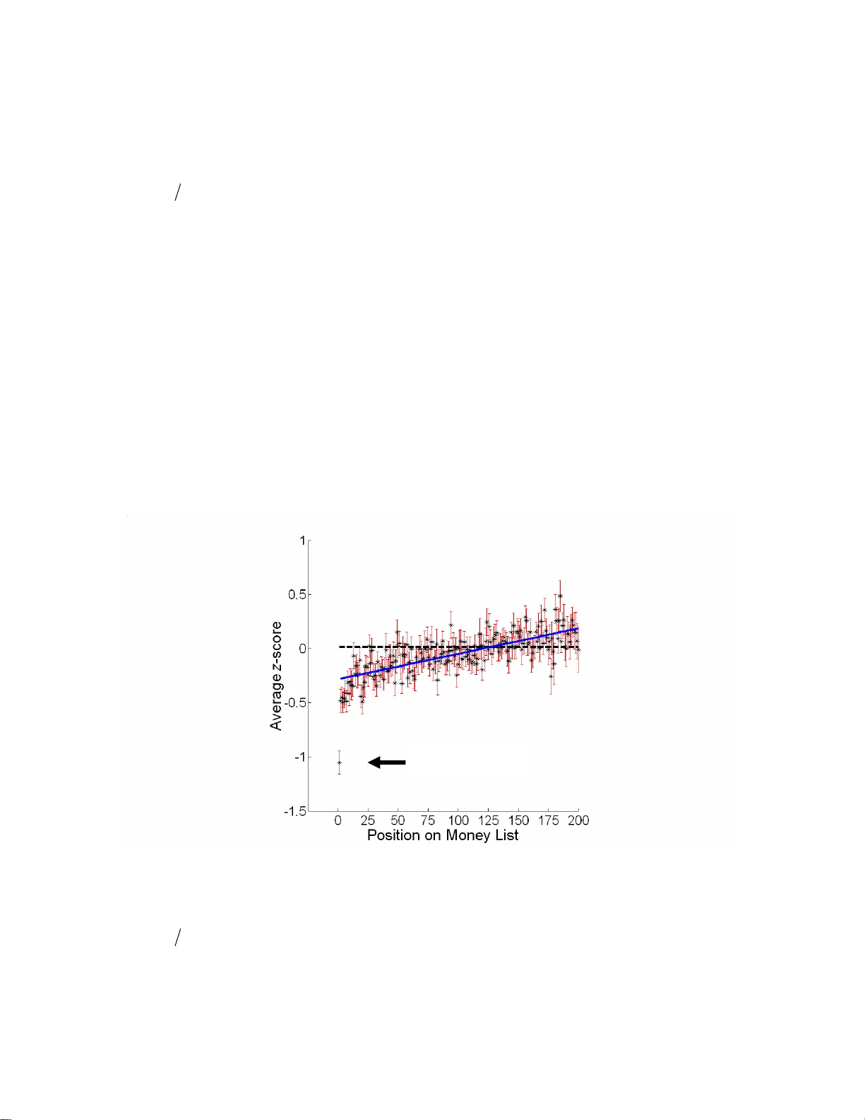
PGA Tour Scores as a Gaussian Random Variable Robert D. Grober Departments of Applied Physics and Physics Yale University, New Haven, CT 06520 Abstract In this paper it is dem onstrated that the sc oring at each PGA Tour stroke play event can be reasonably modeled as a Gaussian random va riable. All 46 stroke play events in the 2007 season are analyzed. The distributions of scores are favorably compared with Gaussian distributions using the Kolmogorov- Smirnov test. This observation suggests performance tracking on the PGA tour should be done in terms of the z -score, calculated by subtracting the mean from the raw score a nd dividing by the standa rd deviation. This methodology measures performance relative to the field of com petitors, independent of the venue, and in terms of a st atistic that has quan titative m eaning. Se veral examples of the use of this scoring methodology are pr ovided, including a calculation of the probability that Tiger Woods will break Byron Nelson’s reco rd of eleven consecutive PGA Tour victories. Statistical analysis is now a ubiquitous aspect of most professional sports [ 1 ]. Perhaps the best example of this is professiona l baseball, where nearly every aspect of the game is fram ed in terms of statistical analysis [ 2 ]. Professional golf is also a sport that focuses intensely on statistics , as the PGA Tour web site (www.pgagtour.com) m aintains statistics on many aspects of the performance of individual players. The goal of this paper is to demonstrate that the 18-hole sc ores reported on the P GA tour are reasonably described in terms of Gaussian statistics . The scores generated by the field of competitors at each venu e is char acterized in terms of a m ean, μ , and variance, , and the histogram of scores at each venue is accu rately described by the associated Gaussi an probability distribution function. 2 σ The central limit theorem states that if the rando m variable y is the sum over many random variables x i , , where N >> 1, then y will be a Gaussian distributed random variable, i.e. the probability density func tion for y is given as ∑ = = N i i x y 1 ( ) ⎥ ⎥ ⎦ ⎤ ⎢ ⎢ ⎣ ⎡ − − = 2 2 2 2 exp 2 1 ) ( y y y y y p σ μ πσ where y y = μ , 2 2 2 y y y − = σ , and the brackets denote an average. Thus, ∑ ∑ = = = = N i x N i i y i x 1 1 μ μ . In the limit the random variables x i are uncorrelated, ∑ ∑ = = = ⎟ ⎠ ⎞ ⎜ ⎝ ⎛ − = N i x N i i i y i x x 1 2 1 2 2 2 σ σ , and thus y μ and are defined by the first and second moments of the random variables x i [ 2 y σ 3 ]. The central limit theorem is i ndependent of the statistics of x i so long as N >> 1. However, in the limit that the x i are well behaved (i.e. not so different than Gaussian), N need not be very large before y is Gaussian. In the limit tha t the x i are Gaussian, the central limit is trivially tr ue even for N ~ 1, as the sum over Gaussian random variables is a Gaussian random variable. The final score of a round of golf is defined by the sum , where x i is the score on the i th hole and N = 18. One might reasonably e xpect the centra l limit theorem to be relevant to the distribut ion of scores at a golf tournament provided the distribution of strokes taken on each hole, x i , are reasonably behaved random variables. This is likely the case for tournaments involving golf profe ssionals, who generally score not too much different from par on each hole. ∑ = = N i i x y 1 As a preliminary test of this hypothesis, the scores reported for the 2007 PGA Tour Qualifying School at Orange Count y National, November 28, 2007 through December 3, 2007 were analyzed. The event involved 158 golfers play ing six rounds of tournament golf. Each golfer played three rounds of golf on each of the two different courses, Panther Lake Course and Crooked Ca t Course. The final results posted online by the PGA tour [ 4 ] do not distinguish between the two courses. Likewise, the analysis does not distinguish between the two courses. The probability distribution of the 948 scores is s hown in Fig. 1. This distribution is calculated by first making a histogram of all the scores. The probabilities are calculated from the histogram by norm alizing th e number of counts in each bin by the total number of scores. The uncertainties are estimated as the square root of the num ber of scores in a particular bin norma lized to the total number of scores, i.e. it is assumed the statistics associated with the num ber of scores in each bin are Poisson [ 5 ]. The resulting probability distribution and estimated uncertain ties are indica ted by the vertical bars in Fig. 1. The first and second moment of the pr obability distribution of scores yield a mean = s μ 70.8 strokes and standard deviation 6 . 2 = s σ strokes. Motivated by the centra l limit theorem , a model for this proba bility distribution is shown as the solid line in Fig. 1. This model distribution is obtained numerically by taking 10 5 samples of a Gaussian random variable with the sam e mean and standard deviation as the data, then rounding each samp le to the nearest integer. Visually, the model seems to be a very reasonabl e representation of the data. Figure 1: The probability distribution of the 948 scores reported for the 2007 PGA Tour Qualifying School. Calculation of the first and second moment yield a mean = s μ 70.8 strokes and standard deviation 6 . 2 = s σ strokes. The vertical bars represent the probability distribution and estimated uncer tainty. The solid line is the m odel distribution. All calculations are described in the text. A standard test of the similarity of two sample populations is the Kolm ogorov- Smirnov ( K-S ) test [ 6 ], in which the cumulative distribution f unctions of the two sam ple populations are compared. The K-S test is designed to test as a null hypothesis whether the two distributions are drawn from the sa me underlying distribution. This type of testing is particularly sen sitive to erro rs in the tails of the prob ability distribution functions. The resulting p -value defines the significance level at which one can reject the null hypothesis. It is standard practice to re ject the null hypothesis at significance levels five percent or less. The K-S test is based on an analys is of the Quantile-Quantile ( QQ ) plot, comparing the cumulative distribution functi ons of the two sam ple populations. One representation of the QQ plot is shown in Fig. 2, in wh ich the inverse of the cum ulative distribution function ( CDF ) for both sample populations, the data and the model, is calculated in 1% increm ents from 1% th rough 100%, yielding 100 data points for each sample population. These two data sets are th en plotted parametrically w ith the model on the ordinate axis and the data on the abscissa axis. Each data poi nt is represented by a cross in Fig. 2. Because many of the point s are o verlapping, each data point in the graphic has been dithered by the addition of a random num ber drawn from a Gaussian distribution with = μ 0 strokes and standard deviation = σ 0.2 strokes. The solid line shown in Fig. 2 is the line x = y , which is what would be observed for two identical sample populations. The QQ plot is very linear, indicat ing the two sample populations are similar. Figure 2: A QQ plot of the raw data and the model data, indicated as crosses. For purposes of presentation, each data point has been dithered random ly by a small am ount so that the density of data points can be appreciated. The solid line is the line x = y , which is what would be observed fo r two identical distributions. The K-S test returns a p - value of 0.92, making it difficult to reject the null-hypothesis that the two samples are drawn from the same distribution. The K-S test is performed using a numeri cal analysis provided in MATLAB [ 7 ]. Because the resulting p -value is 0.92, the null hypothesis can not be rejected. Thus, it is convincing that the scores are reasonably re presented as a Gaussian random variable. This analysis was performed for the 46 str oke play tournam ents held as part of the 2007 PGA Tour from January 4 thru November 4, (including the Masters Tournament, United States Open Championship, British Open Cham pionship, and PGA Championship) using the scor es reported on the PGA tour web site, www.pgatour.com. For each event, the first and second moments ar e calculated, yi elding mean and variance. The probability distribution of the scor es is calcu lated and the resulting CDF is compared in a K-S test to the CDF of the corresponding model function. This analysis results in a p -value for each of the 46 tournaments. The CDF of this distribution of p -values is indicated in Fig. 3 as the crosses. Wh ile the great majority of p -values are p > 0.7, there is a significant ta il that extends to values p < 0.2. Fig. 3: Shown as crosses is the cumulative distribution of p -values obtained by performing a K-S analysis for each of the 46 tournam e nts, comparing the scores to the model function. The solid line is the cumulative distribution of p -values obtained by simulating the results of the 46 tournaments using the m ean, standard deviation, and total number of scores for the actual events; assum i ng the scores are distributed as a Gaussian random variable; and then itera ting the process 100 times. To understand this distribution of p -values, the following numerical model was considered. All 46 tournaments were simulated assum ing the scores to be distributed as a Gaussian random variable with mean, standa rd deviation, and to tal number of scores corresponding to the actual events. The resul ting sampling of scores were compared in a K-S test against the model function, which consists of 10 5 Gaussian distributed samples of the same mean and standard deviation. This process was then iterated 100 tim es, i.e. as if running the PGA tour for 100 years, resulting in 4600 p -values. The CDF of these p -values is shown as the solid li ne in Fig. 3. One can use a K-S analysis to compare the CDF of this model distribution of p -values with the CDF of p -values obtained from analysis of the 46 tournaments. This analysis yields p ~ 0.80, making it very difficult to reject the null- hypothesis that all scores on the PG A tour are drawn from Gaussian distributions . Fig. 4: The average score (a bscissa) plotted parametrically against the standard deviation (ordinate) for each of the 46 stroke play tourna ments. The error bars are estim ates of the uncertainty, as described in the text. The so lid line is a linea r fit of the data, yielding a slope of 0.12. This indicates that more di fficult golf courses do a s lightly bette r job of separating the better players from the poorer players. The strength of this analysis is that o n e can separate the perform ance of the field of competitors f rom the difficulty of the venue. As a first example, shown in Fig. 4 is the mean score ( s μ ) plotted vs. the standard deviation of the scores ( s σ ) for all 46 tournaments. The uncertainties are represented as error bars and estim ated as N s σ , where N is the number of scores reported for ea ch tournam ent. Note that the Masters Tournament and the U.S. Open Championshi p have anomalously high m ean scores, 75.1 strokes and 76.2 strokes respectiv ely. The solid line is a linear fit to the data and has a slope 12 . 0 = Δ Δ s s μ σ . This line highlights the trend of increasing s σ with increasing s μ , indicating that harder course s do a little better at separa ting the better players from the rest of the field. The most popular methods for com paring the overall perform ance of competitors on the PGA tour are the money list and the scor ing average. This analysis suggests an alternative method for comparing performa nce, where in one keeps track of the z -scores for each competitor. The z -score, sometimes called either standard score or norm al score, is a dimensionless measure of the difference f rom the mean in te rms of the number of standard deviations. It is calculated b y subtracting the mean from the raw score and dividing by the standard deviation. The z -score is a standard statistical tool used for comparing observations from di fferent norm al distributions [ 8 ]. The z -score methodology applied to scores on the PGA tour would allow one to understand how individual players perform rela tive to the field, independe nt of the difficulty of the courses. Additionally, the z-sco re characterizes p erformance in term s of a statistic that has quantitative meaning. Several examples of the uses of this methodology are provided in the following paragrap hs. Z -scores were calculated for all players re turning scores in the 46 events o n the 2007 PGA tour. The average z -score, z μ , for each player was then calculated, along with the corresponding standard deviation of the z -score, z σ , for each player. These z μ are plotted in Fig. 4 as a function of the player’s position on the 2007 PGA Tour money list for the top 200 players on the m oney list. The star indicates z μ and the vertical error bar indicates the uncertainty in our es timate of z μ , which we approximate as N z σ , N being the total number of scores reported fo r the player in 2007. There are several interesting things to note in this graphic. First, the resulting curv e is linear with a slo pe position 0023 . 0 . If one assumes 3 ≈ s σ strokes, (see Fig. 4), then one concludes only 0.34 strokes per round separate a 50 place di fference in position on the money list. Second, the cut at the 125th player for cont inued exemption on the PGA tour occurs very near to z μ = 0. Thus, competitors playing better than the average of the field will likely keep their PGA tour exemption. Finally, z μ for the first player on the money list, Tiger Woods, stands alone. His z μ is approximately 1.05, while his closest com petitors have z μ ~ 0.5. This amounts to Mr. Woods typically being in the top 15% of the field on any given day, while his closest co mpetitors are typically in the top 30% of the field. Tiger Woods Fig 5: The vertical bars a nd stars represent the average z -score for each of the top 200 players on the 2007 PGA tour money list. The solid line is a linear fit to the z-scores of all but the first ranked player on the money list. The sl ope of the solid line is position 0023 . 0 . The dashed line is the value of z μ corresponding to the 125th position on the money list, which corresponds very nearly to z μ = 0. The number one ranked player on the money list, Tiger Woods, has ~ 1. z μ 05, which is anomalously low in parison to all other pl com ayers. Another use of the z -score is to track the perfor mance of individual players over me. T ti he z -scores for each player on the 2007 P GA tour were charted chronologically. A linear fit was then perform ed on the data as a means of identifying trends. Based on this analysis, Justin Leo nard was the most im proved player of the top 125 players on the money list. His z -scores are shown in Fig. 6, plo tted chronologically. His average z - score z μ is 12 . 0 − , and is indicated by the dashed line. The linear trend, indicated as solid line, suggests he improved by almo st a full standard deviation, from the z μ = 41 . 0 to z μ = 62 . 0 − over the course of the year. Assuming 3 ≈ s σ , this amounts to an t of three strokes per rou nd over the course of the year. improvemen Fig 6: The z -scores for Justin Leonard, arranged ch ronologically, for all rounds he played on the 2007 PGA tour. His average z -score is 12 . 0 − = z μ , and is indicated by the dashed line. The linear trend, indicat ed as the solid line, suggests that he improved by almost a full standard deviation, from 41 . 0 = z μ to 62 . 0 − = z μ over the course of the year. Based on this analysis, Justin L eonard was the most improved player of the top 125 players on the 2007 money list. It is worth noting that the third most improved player in 2007 was Tiger Woods. His z -scores are charted chronologically in Fig. 7. While his average z -sco re z μ is 05 . 1 , − the linear fit suggests he improved by 2/3 of a standard deviation, from 64 . 0 − = z μ to 33 . 1 − = z μ , over the course of the year. This amounts to an im shots per round. Relevant to the followi ng analysis, it is notable that he o -scores less than or equal to 5 . 1 provement en has of two clusters of ft z − , and occasionally has clusters exceeding 0 . 2 − . Fig 7: Z -scores for all 2007 scores reported for Tiger Woods, arranged chronologically. While his average z -score is 05 . 1 − z μ , the linear fit sugge sts th at he improved by 2/3 of a standard deviation, from 64 . 0 − = z μ to 33 . 1 − = z μ , over the course of the year. Based urnaments. As an example, we have calcula ted the probability tha t a fictitious player on this analysis, Tiger Woods was the third most im proved player of the top 125 players on the 2007 money list. Finally, one can use the z -scores in a statistical analysis to pr edict the outcome of to will tie or break Byron Nelson’s long standing record of eleven consecutive PGA Tour victories over the course of a 300 tournament career. This ca lculation was chosen so as to inform the ongoing speculation as to whether T iger Woods will break this reco rd in th remaining years of his career. For the purpos es of this calculation, his rem aining career is assumed to span 300 tournaments, i.e. 20 tournaments per year for the next 15 years. The calculation is as follows. The field of competitors is defined by the ensem ble of e z μ and z σ indicated in Fig. 5, excluding thos e of Tiger Woods. A tournament is si ed by assuming the players comprise th e top 155 competitors in the field plus a fict us co etitor. This fictitio us competitor is assigned a value of mula itio t mp z μ and z σ . Th particular value of e z σ is that of Tiger Woods, which is calc ulated using the data in Fig. As is discussed below, 7. z μ for this fictitious player is fi xed for the dura n of t career, and various different careers are modeled by changing the value of tio he z μ . Using this ensemble of z μ and z σ , and a Gaussian rando m number generator [ 9 ], a tournament is simulated by generating four scores for each player. The to tal for each player is calculated, th esult the virtual tournament is tabula ted, and it is deter mined if the fictitious competitor wins the event. The career of this fictitious com petitor is modeled as the results for 300 simula tournaments. The total number of win e r of ted s a nd the maximum number of consecutive wins r the fo competitor is tabulated. Each career is then run 10 4 times to improve the resulting statistics. This is then done for various values of z μ , so as to gauge how the results vary as a function of z μ . Figure 8: The probability of our fictitious com petitor winning a tournam ent as a function of z -score. Details of the calculation are descri b ed in the text. The crosses indic ate the calculated data points. The solid lin e is draw n as an aid to the eye. Note that the probability approaches 0.5 as z μ approaches 5 . 1 − . The graphic in Fig. 8 indicates the probabi lity of victory in a tournament for the fictitious competitor as a function of z μ . The data are indicated by the crosses. The solid line connects the data points as an aid to the eye. The probability of victory is approximately 1 in 40 for z μ = -0.5, rising to approximately 1 in 2 for z μ = -1.5. The graphic in Fig. 9 indicates the probabi lity that the f ictitious comp etitor wins eleven or more consecutive tournaments over the course of a career, as a function of z μ . The data are indicated by the crosses. The so lid line connects the data points as an aid to the eye. The graphic shows the pr obability to b e negligible for z μ as low as . In order to have even odds of achieving eleven or more consecutive victories, the fictitio us competitor requires a value of 5 . 1 − z μ approaching 0 . 2 − over the course of the entire 300 tournament career. As shown in Fig. 7, Mr. W oods occasionally has perio ds of play with z μ as low as -2.0; however, the existing data does not support the no tion that this level of performance can be maintained over the course of a 15 year career. At the very least, it provides Mr. Woods with a cha llenging and quantitative goal. Figure 9: The probability of eleven or more consecutive wins as a function of z μ over the course of a 300 tournament career. Details of the calculation are de scribed in the text. The crosses indicate the calculated data poin ts. The solid line is drawn as an aid to th e eye. Note that the probability approa ches even odds as the value of z μ approaches . 0 . 2 − In summary, it has been demonstrated th at the scores generated on the PGA tour are reasonably modeled in terms of Gaussian s tatistics. This analysis sugg ests the z -score is a valuable alternative methodology for m easuring performance on the PGA tour, as it provides a means of measuring performance rela tive to the f ield of competitors that is independent of the relative di fficulty of the various tourna ment golf courses. As an example of this methodology, the z -score was used to iden tif y the most improved player on the 2007 PGA tour to be Jus tin Leonard. Additionally, the z -scores are used to simulate the career of a fictitious play er in an attempt to infor m speculation as to the likelihood Tiger Woods will be ab le to equal or better Byron Nelson’s record of eleven consecutive PGA tour victories. This anal ysis suggests a player must m aintain an average z -score of order for the duration of a 15 year ca reer in order to have even odds of breaking this record ; a feat that seems extrao rdinarily challenging. 0 . 2 − Acknowledgements: The author acknowledges useful conversations with and thoughtful advice from Professor Joseph Chang of Yale University and Professor W illiam Press of University of Texas at Austin. References and Endnotes 1. J. Albert (Ed.), Jay Bennett (Ed.) and J.J. Cochran (Ed.), Anthology of Statistics in Sport, ( ISBN- 13: 978-0-898715-87-3, Society for Industrial and Applied Mathematics, 2005 ). 2. G. Gillette (Ed.) and P. Palmer (Ed.), The ESPN Baseba ll Encyclopedia (ISBN-13: 978-1402725685 , Sterling, 2005). 3. For a discussion of the Central Lim it Theorem, see F. Reif, Fundamentals of Statistical and Thermal Physics, (McG raw-Hill Book Company, New York, 1965), pp 37-40. 4. Results for the 2007 qualifying school are posted at www.pgatour.com/qschool/leaderboard. 5. For a discussion of Poisson processes, see F. Reif, Fundamentals of Statistical and Thermal Physics, (McGraw-Hill Book Co mpany, New York, 1965), pp 41-42. 6. W.H. Press, B.P. Flannery, S.A. Teukol sky, and W.T. Vetterling, Numerical Recipes (Cambridge University Press, New York, 1989), Chapter 13.4 – 13.5, pg 464 – 475. 7. The MATLAB function call is ‘kst est2’. Details can be fou nd at www.mathworks.com. 8. John E. Freund, Modern Elementary Statistics , 5th ed., (Prentice-Hall, New Jersey, 1979), pg 191. 9. It has not been de monstrated here that the z -scores for a particular player are Gaussian distributed. However, for the purposes of this specula tive ca lculation, it is probably a reasonable assumption.