On capacity of wireless ad hoc networks with MIMO MMSE receivers

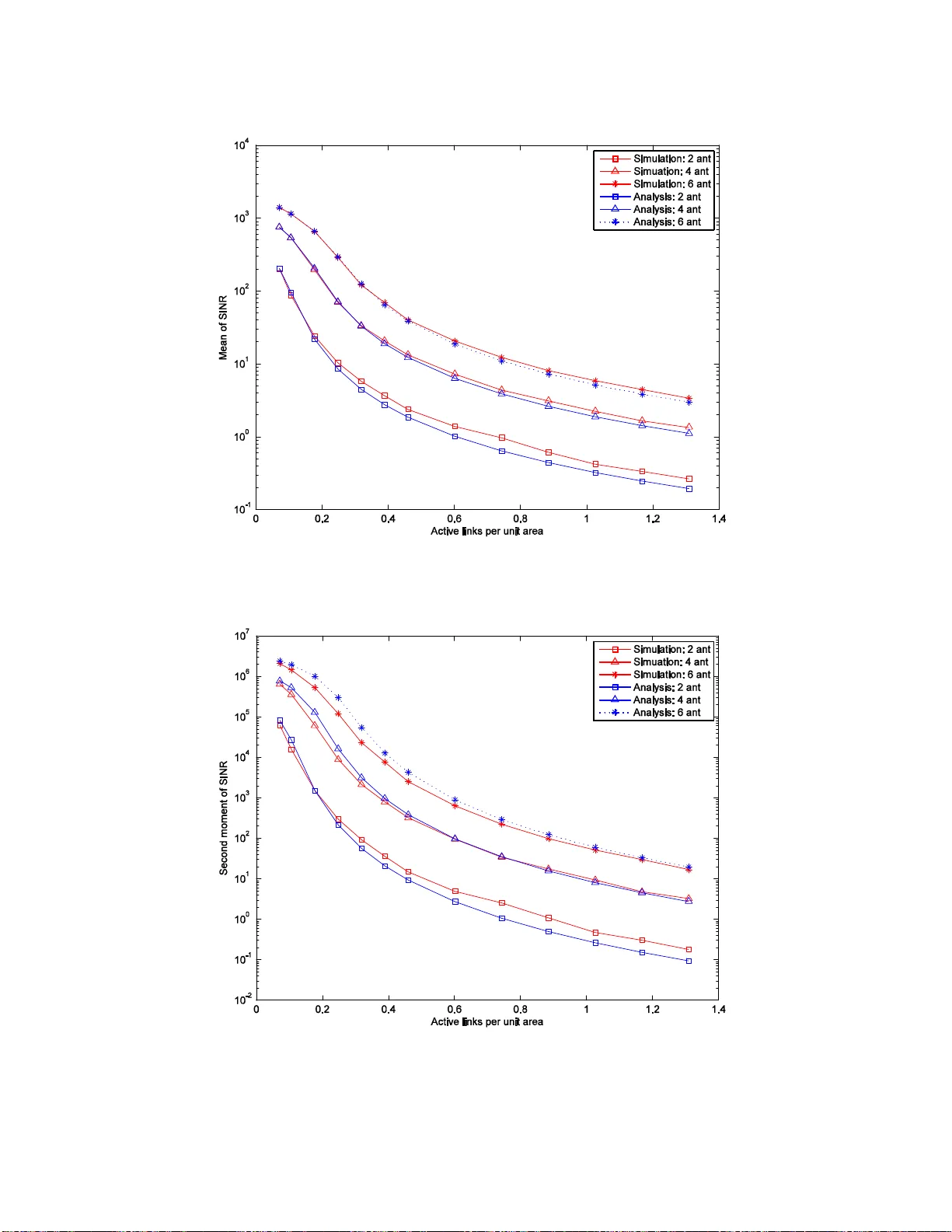
On Capacity of Wireless Ad Hoc Ne tworks with MIMO MMSE Receivers Jing Ma, Member, IEEE and Ying J un (Angela) Zhang, Member, IEEE Dept. of Information Engineering, The Ch inese University of Hong Kong, Hong Kong Email: mjingq@gm ail.com,yjzhang@ie.cuhk.edu.hk Abstract - Widely adopted at home, business places, and hot s pots, wireless ad-hoc networks are expected to provide broadband services parallel to their wired counter parts in near future. To address this need, MIMO (multiple-input-multiple-output) techniques, which are capab le of offering several-fold increase in capacity, hold significant promise. Most previous work on capacity an alysis of ad-hoc networks is based on an i mplicit assumption that each node has only one antenna. Core to the an al ysis therein is the characterization of a geometric area, referred to as the exclusion region, which quantizes the am ount of spatial resource occupied by a link. When multiple antennas are deployed at each node, however, multip le links can transmit in the vicinity of each other simultaneously, as interference can now be suppressed by spatial signal processing. As such, a link no longer exclusively occupies a geometric area, making the concept of “exclusion region" not applicable any more. This necessitates a revisit of the fundamental understa nding of capacity of MIMO ad-hoc networks. In this paper, we investigate link-layer throughput capacity of MIMO ad-hoc networks. In contrast to previou s work, the amount of spatial resource occupied by each li nk is characterized by the actual interference it im poses on other links, which is a function of the correlation betw een the spatial channels, the distan ce between links, as well as the detection scheme at the receivers. To calculate the link-layer capacity, we first derive the probability distribution of post-detection SINR (si gnal to interference and noise ratio) at a receiver. The result is then used t o calculate the number of active links and the corresponding da ta rates that can be sustained within an area. Our analysis shows that there exists an optimal active-link density that maximizes the link-la yer throughput capacity. This will serve as a guideline for the design of medium a ccess protocols for MIMO ad-hoc networks. To the best of knowledge, this paper is the first attem pt to characte rize the capacity of MIMO ad-hoc networks by considering the actual PHY-layer signal and interference model. The r esults in this paper pave the way for further study on network-layer transport capacity of ad-hoc networks with MIMO. Key words: Wireless ad hoc networks, MIMO, Network capacity. I. I NTRODUCTION MIMO (Multi-Input Multi-Output) sy stem s where multiple antennas are deployed at both transm itter and receiver, open up a new dimension, i.e., space, to significantly improve the spectral efficiency of wireless communication system s. Fosc hini and Telatar [1]-[2] show that MIMO provides a linear growth of capacity with the number of an tennas. Moreover, the extra degree of freedom, i.e., space, of fered by multiple antennas enables in terference cancelation at receiving stations, which a llows spectrum to be reused more aggressively [3]-[7]. On the other hand, MANET (mobile ad hoc network) is likely to play a major role in next-generation home networks and hot spots, thanks to its simplicity, cost effectiveness, and simple reconfiguration [8]. One of the major challenges faced by MANET is the increasing demand for data-rate-intensive applications similar to thos e in its wired counterpart. Deploying multiple antennas at each node is a promising solu tion to improve netw ork capacity and link reli ability required by these applications. To fully exploit the be nefits of MIMO in ad hoc networks , it is essential to have a thorough understanding of the fundamental impact of th e use of MIMO on overall network performance. Most previous work on capacity analysis of ad hoc networks is based on an implicit assumption that only one antenna is used at each node [9]. Under th is assum ption, an active link exclusively occupies a geometric area, referred to as the exclusion region, to avoid collisions with other links. The larger the exclusion region, the more spatial resource a link occ upies, and the capacity of a network is essentially determined by the amount of spatial resource occ upied by underlying links. When multip le antennas are deployed at each node, however, an active link no longer exclusively occupies a spatial area, making the original definition of “exclusion region" no t applicable any more. In fact, m ultiple adjacent links can transmit at the same tim e, as long as the mutu al interference can be s uppressed by spatial signal processing. As such, previous work on capacity analysis is not directly applicable to ad hoc networks with MIMO links. The impact of multiple antennas on network capacity was previously studied under different contexts. In [23]-[24], Zhang and Li ew derived the upper and lower bounds on network capacity when directional antennas with realizable generic pa tterns are used. It is well known that directional antennas do not work well in indoor and urba n environments where a large num ber of local scatterer s cause severe m ultipath effects and large angular spread. Unfortunately, most application scenarios of ad hoc networks perceive rich-scattering channels. As a result, the previous analysis based on directional antennas does not apply to general MIMO ad hoc networks. In [15], Chen et al studied the ergodic singl e-hop capacity of ad-hoc networks when single-u ser detection is employed at each receiver. Though simp le, single-user detectors do not exploit the interference cancelation capa bility of MIMO. As a result, the capacity calcu lated in [15] is far below the actual achievabl e capacity of MIMO ad hoc networks. In this paper, we investigate link- layer throughput capacity, defined as the total da ta rate that can be successfully delivered thr ough all single-hop links within a unit ar ea, of MIMO ad-hoc networks. In particular, MMSE (minimum m ean square error), th e optimal linear multiuser detection, is assumed to be deployed at receiving nodes, as it has the highest interference suppression capabilit y among all linear detection schemes including ZF (zero forcing) and sing le user detectio n [25]. In contra st to previous work, we characterize the amount of spatial reso ur ce occupied by each link by the actual interference active links im pose on each other, taking into consid era tion the actual behavior of multipath fading and MIMO systems. One of the key challenges in this work is the ch aracterization of the dist ribution of post-detection SINR (signal to interference and nois e ratio) when transmitte rs are randomly located. SINR distr ibution of MMSE detectors was previously studied in [26] -[28], [19]. In [27] and [28], the authors proved asymptotic Normality of post-detection SINR for equal and non-equal interference power, respectively. In [19], Li et al improved the accuracy by m ode ling SINR using a Gamma or a generalized Gamma distribution. All these papers assumed that the signal strength of interfering data stream s as detected at the receiver is deterministic and known. In ad -hoc netw orks, however, active nodes are randomly located, and hence the received interference power is also random. Moreover, previous work often assumed that the number of interferer s is smaller than or comparable to th e number of receive antennas. While the assump tion is reasonable for traditional cellu lar networks, it is not tr ue in ad hoc networks where the number of simultaneously transm itting stati ons could be much larger than the number of antennas at a receiving node. The ma in contributions of this pape r can be summarized as follows. • We derive a closed-form expression for the distri bution of received SINR of an active link with maximum ratio transm ission and a multiuser MMSE receiver. In contras t to [26]-[28], [19], signal power, interference power, and the number of interferers are all random variables due to the randomness in the location and activity of transmittin g nodes. The analytical results are validated by nume rical sim ulations. • Based on the SINR distribution, we analyze link-layer throughput capacity, calculated as the sum data rate that can be delivered by all links within a unit area. In contrast to [15] where the data rate of each link is represen ted by ergodic capacity, per-link data rate is defined as in this paper, where is the transmission rate of each lin k and is the =( 1 ) out Th P q − q out P probability of transmission failu re given . This definition more accurately re flects the characteristics of today's ad-hoc networks, wher e multipath fading varies slowly compared with the transmission time of a packet. Unlike the m ean value analysis in [19], the PDF (probability density function) of SINR is needed in this paper to calculate , which makes the job here much more challenging. Our work on link-laye r capacity paves the way for further study on network-layer transport capacity of ad-hoc networks with MIMO links. q out P • The analysis suggests that there exists an optim al density of simultaneously transmitting link s that maximizes the link-layer capacity. Thro ugh num erical study, we calculate the optimal density under various scenarios. In real implementation, the op timal active-link density can be mapped to an optimal transm ission probability in the MAC (medium access control) layer. Th is result serves as a guideline fo r the design of MAC protocols of next-generation ad-hoc networks with MIMO links. • Our analysis is based on the as sumption that CSI (channel state information) from all transmitting nodes to th e receiver of a tagged link is available at the receiver. In practice, it is likely that a receiver only knows CSI from a few neighboring links. In this paper, we also study the link-layer capacity and the corresponding op timal link density when only local CSI is available. The remainder of the paper is organized as follows. The system and signal models are presented in Section II. In Section III, we deri ve the distribution of post-detection SINR in ad hoc networks when MMSE receivers are deployed. The link-layer thr oughput capacity is then given in Section IV. Numerical examples and discussion s are presented in Section V, wh ere we also study the impact of partial CSI on the capacity and optimal link densit y. Finally, the paper is c oncluded in Section VI. II. S YSTEM M ODEL We first describe the notation used in this paper for readers' convenience. Throughout the paper, scalars are given by normal letters, vecto rs by boldface lo wer case letters, and matrices by boldface upper case letters. Besides, the following notations are used. T X : Transpose operation * X : Hermitian transpose [] ij X : th element of (, ) ij X Tr ( ) X : trace of matrix X E( ) i : Expectation Var ( ) i : Variance A. System Description Consider an ad hoc network as demonstrated in Fig. 1, where mobile nodes are uniform ly distributed within an area. Each node is equipped with antennas. For simplicity, we ignore the edge effects and assume that each link has the sam e statistical character istics. W ithout loss of generality, let Link 0 be the tagged link. At a given time, there are other links sending data at th e same time as Link 0, resulting in co-channel interference. As a result, the data received by the tagged link, given as follo ws, is a superposition of desired signa l, interference, and noise. m K 00 0 0 0 =1 = K kk k k k pp αα 0 + + ∑ y Hx Hx n (1) In the above, is an mm channel m atrix, representing the chann el fading from the transm itter of the th link to the receiver of the tagged link. Assuming a rich scatteri ng environm ent and quasi-static Rayleigh flat fading channels, we can model the elem ents of as i.i.d. comple x Gaussian random variables. Likewise, denotes the transmit signal vector of Link ; k H × k k H 0 x k k p the transmit power of Link ; k k α the path loss from the transmitte r of Link to the receiver of the tagged link; and the AWGN (additive white Gaussian noise) with ze ro mean and unit variance. k 0 n Note that the number of inte rferers, , is a random variable de pending on the transmission probability of links. Since the neighborhood observed by each link is statistically identical, we assume that the interferers are randomly located within a disc of radius K K R centered at the tagged receiver, where R is the largest distance at which an interferer can cause non- negligible inte rference to the receiver. Furthermore, let ε denote the minimum separation betw een interferers and the tagged receiver. Assume that ε is small enough so that it does not affect the unifor m distribution of nodes. Thus, the probability density functi on of the distance between a node an d the tagg ed receiver is given by 22 2 () = d x fx R ε − (2) Let be the distance between the th transmitter to the tag ged receiver and k c k θ be the path loss exponent. In particular, is the length of the tagged link. We can calculate the received power from the th interferer as 0 c k 0 00 =( ) kk k c p p c θ αα (3) whose PDF is 2/ 2 00 0 0 0 00 00 22 ( 2 ) / 2( ) () = ( ) ( ) . () p kk pc c c f xp Rx R θ θθ α θθ α αα θε ε + ∀≤ ≤ − x p (4) When =4 θ , 2 00 0 44 00 00 00 22 3 / 2 () = ( ) ( ) 2( ) p kk pc cc f xp Rx R α α αα εε ∀≤ ≤ − x p j v r (5) B. Maximum Ratio Transmission and MMSE Reception It was proved in [29] that SVD (singular value decomposition) based space-tim e vector coding allows the collection of signal power in space and it is a th eo retical means to achieve high capacity for MIMO systems. By SVD, can be decomposed into k H (6) * ,,, =1 =, r k kk j k j k j λ ∑ Hu where ,1 , 2 , kk k k λ λ ≥≥ ≥  λ are the eigenvalues, and are the left singular vector and right singular vector, respectively, and is the rank of . Note that the left an d right singular vectors have the same distribution as no rmalized complex Gaussian random vectors [20]-[21]. Likewise, the distribution of the square of the largest singular value , kj u H , kj v 2 ,1 k k r k λ is given by [17] as a finite linear combination of elem entary Gamma densities: 2 1 22 2, ,1 =1 = 0 () = > 0 , ! ll n x mm n n nl k nl nx e fx g x l λ +− − ∀ ∑∑ (7) where are computed and listed in [17] for most antenna confi gurations of interest. The , nl g τ th moment of 2 ,1 k λ is () 2 22 , 2 ,1 =1 = 0 () E[ ] = . ! mm nn nl k nl gl nl τ τ ! τ λ − + ∑∑ (8) In an interference-lim ited environm ent such as ad hoc netw orks, an active link should transmit only one data stream at a time to optimize the sy stem pe rformance [11]-[13]. In this case, the sin gle data stream should be transmitted on the largest singular m ode of the channel for SNR (signal to noise ratio) maximization. Such scheme, known as MRT (maxim um ratio transmission), configures the transmit antenna weight using the right singular vector corre sponding to the domi nant singular value. 1 For example, the transmit antenna weight of Link 0 is . Similarly, the transmit beamforming vector of Link , denoted by , is the dominant singular vector o f the channel matrix between its own transmitter-receiver pair. Therefore, th e received signal in (1) becomes 0, 1 v k k t 00 0 0 0 , 1 0 =1 = K kk k k k k pb p b αα 0 + + ∑ y Hv Ht n 00 0 , 1 0 , 1 0 0 =1 ˆ = K kk k k k pb p b αλ α + + ∑ uh n (9) where 0 y is a vector with the th element being the received signal on the th receive antenna. Denote by , whose elements are still i.i.d. c omple x Gaussian random variable s with zero mean and unit variance [2], since has unit norm and is independent of . 1 m × ˆ k h i i kk Ht k t k H Define equivalent channel matrix as G (10) 0, 1 0, 1 1 ˆˆ =[ , , , ] , K λ Gu h h  and the transmit pow er matrix as 00 11 =. KK p p p α α α ⎡ ⎤ ⎢ ⎥ ⎢ ⎥ ⎢ ⎥ ⎢ ⎥ ⎣ ⎦ P  (11) We can then rewrite (9 ) into a matrix form as 1/ 2 00 =, + y GP b n (12) where is . b 01 [,, , ] T K bb b  Upon receiving the signal, the tagged receiver attem pts to obtain an estim ate of from the received signal b 0 y . Being the optimal linear detector, MMSE detect or m inimizes the mean square error between and its estimate. Specifically, th e decision statistic s b is obtained by lin early combining the received signal vector as follows: b  1 To implement MRT, transmitter-side CSI is needed. Transmitte r-side CSI is easily achievable in wireless n etworks with two-way com munications. I n case it is not available, ra ndom antenna selection or space time codi ng can be deployed instead of MRT. Our analysis can be easily extend ed to these cases with slight modification. Specifically, it is the distribution of 0, 1 λ that needs to be modified in the analysis. * 0 = bV y  (13) where and () 1 * 1 = K − + + VI G P G G P 1 K + I is a ( 1) ( 1) KK + ×+ Identity matrix. W ith MMSE, the post-detection SINR of the tagged link can be calculated as [25] () 0 1 * 1 1, 1 1 SI NR = 1 K − + − ⎡⎤ + ⎢⎥ ⎣⎦ IG P G (14) where den otes the element of a m atrix. The distributi on of SINR was previously studied in [26]-[28], [19]. However, their work assumes that interference power (i.e., 1, 1 [] ⋅ (1,1) th kk p α for ) is deterministic and known. This assumption, however, is not applicable to ad hoc networks where interfering links are randomly located. In this pa per, we focus on MMSE receivers, for it achieves the optimal performance in term s of BER (bit error rate) or SINR among all linear detectors. Our conclusions, however, can easily be extended to other suboptimal detectors such as ZF (zero forcing) and single-user detection. >0 k Note that eqns. (13) and (14) have assumed that the tagged receiver has the knowledge of for all . Although not realistic, this assumption allows us to investigate the fundamental lim it of wireless MIMO network capacity without taki ng into account implementation deta ils. This assumption will later be removed in Section V in Fig. 8 and Fig. 9, where the receiver only knows the CSI from its neighboring interfering nodes. ˆ k h k III. SINR D ISTRIBUTION OF MMSE In this section, we derive th e distribution of SINR in ad hoc networks when MMSE detection is deployed. To this end, we first compute the m ean and variance of SINR in subsections III.A to III.E. The PDF of SINR is then presented in III.F. A. Simplified Form of SINR We define 1/ 2 = GP G  000 , 1 0 , 1 1 1 1 ˆˆ =, , , KK K pp p αλ α α ⎡⎤ ⎣⎦ uh h … . (15) and then have 2* * 00 0 , 1 000 , 1 0 , 1 1 ** 10 , 1 0 , 1 1 1 = pp αλ α λ λ − −− − , ⎡ ⎤ ⎢ ⎥ ⎢ ⎥ ⎣ ⎦ uG GG Gu G G     (16) where is G with first column removed. 1 − G   Before going further, we first describe the following lemma. Lemma 1 : Write a matrix into A * 1, 1 1, 1 1, 1 1, 1 =, aa a − −− − ⎡ ⎤ ⎢ ⎥ ⎣ ⎦ A A (17) where is the element of , 1, 1 a (1,1) th A 1, 1 a − is the first column of with the first elem ent removed and is with the first column and row removed. Then, A 1, −− A 1 A ( ) 1 1* 1 1, 1 1, 1 1, 1 1, 1 1, 1 [] = ( ) aa a . − −− −− − − − AA (18) By using Lemma 1, (14) can be simplified as () 0 1 * 1 1, 1 1 SI NR = 1 K − + − ⎡⎤ + ⎢⎥ ⎣⎦ IG G  ( ) 1 22 * * * 0 0 0, 1 0 0 0, 1 0, 1 1 1 1 1 0, 1 =. K pp αλ αλ − −− − − −+ uG I G G G u    (19) Denoting the SVD of as 1 − G  (20) 1 =, − GW D Z  where the i th diagonal element of is , we then can derive the SINR as D i d ( ) 1 22 * * * * * 0 0 0 0 ,1 0 0 0 ,1 0 ,1 0 ,1 SI NR = K pp αλ αλ − −+ uW D Z I Z D D Z Z D W u * ( ) ( ) 1 2* * 1 1 * 0 0 0, 1 0, 1 0, 1 = mm p αλ − −− −+ uW I I D D W u 2* * 1 * 00 0 , 1 0 , 1 0 , 1 =( ) m p αλ − + uW I D D W u (21) 2* 00 0 , 1 0 , 1 0 , 1 = p αλ uB u , where is defined as . B *1 * () m − + WI D D W B. Conditional Mean of SINR It is easy to see that is deterministic function of and . Given a channel realization, the conditional mean of given is B 0 NR G P SI B (22) 2* 0 0 0 0,1 0 ,1 0 ,1 E( S I N R | ) = E( )E( ) . p αλ Bu B u j Likewise, * * () () * () ( ) 0 ,1 0 ,1 0 ,1 0 ,1 0 ,1 0 ,1 =1 E( ) = E E m ii i j ii ij ii j uu B uu B ≠ ⎛⎞ ⎛⎞ + ⎜⎟ ⎜⎟ ⎝⎠ ⎝⎠ ∑∑ uB u () ( ) () 2 * () ( ) 0, 1 0, 1 0, 1 =1 =E | | E m ii ii ij ii j B uu B ≠ + ∑∑ u () *( ) ( ) 0, 1 0, 1 1 =T r ( ) E ij ij ij uu B m ≠ + ∑ B (23) where ij B is the th element of , and is the th element of . Since is a normalized complex Gaussian random vector as mentioned in Section II, it is not dif ficult to prove that ( , ) ij B () 0, 1 i u i 0, 1 u 0, 1 u ( ) *( ) ( ) 0, 1 0, 1 E= 0 ij uu i j . ∀ ≠ (24) Hence, we have the conditional expectation of given as shown in (25). 0 SIN R B () ( ) 1 2* 00 0 0 , 1 1 E( S I N R | ) = E( )Tr m p m αλ − + BW I D * D W () ( ) 1 2* 00 0 , 1 1 =E ( ) T r m p m αλ − + ID D 2 00 0 , 1 2 =1 11 =E ( ) 1 m i i p md αλ ⎛⎞ ⎜ + ⎝⎠ ∑ ⎟ m j (25) C. Conditional Second Moment of SINR We now derive the condition al second mom ent of SINR given . B Denoting as , and () 4 0, 1 E( | | ) (1 ) i ui ≤≤ 1 a () 2 ( ) 2 0, 1 0, 1 E( | | | | ) ( ) ij uu i ≠ as , respectively, we firs t derive (26) from (23). 2 a () * 2 () 4 * () 2 ( ) 2 * () 2 ( ) 2 * 0 ,1 0 ,1 0 ,1 0 ,1 0 ,1 0 ,1 0 ,1 =1 E ( ) = E( | | ) E( | | | | ) E( | | | | ) m ii j i j ii ii ij ij ii jj ii j i j u B B u uB B u uB B ≠≠ ++ ∑∑ ∑ uB u ( ) ( )* ( )* () ** 12 1 2 0, 1 0, 1 0, 1 0, 1 11 2 2 ,, , 11 2 2 1 2 1 2 E( ) ij j i ij i j ij i j i i jj uu u u B B ≠≠≠≠ + ∑ () 4 * () 2 ( ) 2 * () 2 ( ) 2 * 0, 1 0, 1 0,1 0, 1 0, 1 =1 = E (| | ) E (| | | | ) E(| | | | ) m ii j i j ii ii ij ij i i jj ii j i j u B B u uB B u uB B ≠≠ ++ ∑∑ ∑ ** * 12 2 2 =1 =1 = T r( ) Tr ( )T r( ) 2 mm ii ii ii ii ii aB B a a a B B ++ − ∑∑ BB B B * (26) () ** * 21 =1 = T r( ) Tr ( )T r( ) ( 2 ) m ii jj i aa ++ − ∑ BB B B 2 a B B , where the second equality is due to the fact that () ( ) ( )* ( )* () 12 1 2 0, 1 0, 1 0, 1 0, 1 1 1 2 2 1 2 1 2 E= 0 , , ij j i uu u u i j i j i i j j ∀ ≠≠≠≠ (27) Since is a normalized complex Gaussi an random vector, the PDF of is 0, 1 u () 2 0, 1 | i u | 2 2 () 0, 1 ( ) = ( 1)(1 ) , 0 1. m i u fx m x x − − −≤ ≤ (28) Therefore, we have () 2 0, 1 1 E( | | ) = , i u m (29) and () 4 0, 1 2 E( | | ) = . (1 ) i u mm + (30) We can then derive the pdf of on the condition of as () 2 0, 1 | i u | y () 2 0, 1 || = j u 3 22 () ( ) 0, 1 0,1 21 (| ) = 0 1 . 11 m ij uu mx y f xy x y yy − ⎛⎞ −− − ≤ ≤− ⎜⎟ −− ⎝⎠ (31) Then, we have as follows. () 2 ( ) 2 0, 1 0,1 E( | | | | ) ij uu 11 () 2 ( ) 2 0, 1 0, 1 ( ) 2 22 00 || () ( ) 0, 1 0, 1 0, 1 E( | | | | ) = ( | ) ( ) y ij j u ij uu u u xyf x y f y dxdy − ∫∫ 3 11 2 00 21 =( 1 ) ( 1 ) 11 m y m mx y y my x d yy − − − ⎛⎞ −− − −− ⎜⎟ −− ⎝⎠ ∫∫ x d y 1 = (1 mm ) + (32) From eqns. (26) and (32), we have () () *2 * * 0, 1 0, 1 1 E ( ) = Tr ( ) Tr ( )Tr( ) (1 ) mm + + uB u B B B B 22 2 =1 =1 11 1 = (1 ) 1 1 mm ii ii mm d d ⎛⎞ ⎛⎞ ⎛ ⎞ ⎜ + ⎜⎟ ⎜ ⎟ ⎜ ++ + ⎝⎠ ⎝ ⎠ ⎝⎠ ∑∑ 2 ⎟ ⎟ (33) We are now ready to derive the second moment of as 0 SIN R ( ) 22 2 4 * 0 0 0 0 ,1 0 ,1 0 ,1 E( S I N R | ) = E( )E ( ) p αλ Bu 2 B u 22 22 4 00 0 , 1 2 =1 =1 11 1 =E ( ) (1 ) 1 1 mm ii ii p mm d d αλ ⎛⎞ ⎛⎞ ⎛ ⎞ ⎜⎟ + ⎜⎟ ⎜ ⎟ ⎜⎟ ++ + ⎝⎠ ⎝ ⎠ ⎝⎠ ∑∑ 2 . (34) D. Mean of SINR In order to compute the mean of , we first introduce the method of asymptotic analysis of random matrix [18]. 0 SI NR Definition of η transform: Given a nonnegative random variable χ , the η transform is defined as 1 () = E 1 χ ηγ γ χ ⎛⎞ ⎜⎟ + ⎝⎠ (35) Theorem 1 [18] : Let be an mK matrix whose en tries are i.i.d. complex G aussian variables with variance H × 1 m . Let be a Hermitian nonnegative random matrix, indep endent of , whose empirical eigenvalue distribution converges alm ost surely to a nonrandom limit. The empirical eigenvalue distribution of converges almost surely, as with T KK * HTH × H , Km →∞ K m β → , to a distribution whose η -transform satisfies 1 =, 1( ) η β η γη − − T (36) where for sim plicity we have abbreviated * () = η γη HTH . * () η ⋅ HTH and ( ) η ⋅ T stand for the η transform of the eigenvalues of and T , respectively. * HTH Theorem 1 can be applied to find the empirical eigenvalue distribution of , i.e., the empirical distribution of . Rewrite the matrix a s * 11 −− GG  2 i d ** 11 1 1 1 11 =. m mm −− − − − GG G P G  (37) where is with first column rem oved. Then, from Theorem 1, the em pirical eigenvalue distribution of converges almost surely to a distribution whose 1 − P P GG * 1 −−  1 η transform satisfies * 11 * 1 11 1( ) =, 1( ( m K m ηγ ) ) η γη γ −− − −− − − GG P GG   (38) where 1 () m η γ − P is the η transform of the eigenvalue of 1 m − P . We now begin to derive 1 () m η γ − P . Since 1 − P is a diagonal matrix, the empirical eigenvalue distribution of is the distribution of its diagonal elements of 1 − P kk p α . Given the distribution of kk p α in (3), we derive the η transform of 1 m − P as 1 1 () = E 1 m kk mp ηγ γα − ⎛⎞ ⎜⎟ + ⎝⎠ P 22 2 00 0 00 0 00 0 11 22 2 2 =1 tan tan cm p cm p cm p RR α γα γ α εε −− ⎛⎞ −− ⎜⎟ ⎜⎟ − ⎝⎠ γ (39) Substituting (39) to (38), we have 22 00 0 * 00 0 * 11 11 1 * 22 2 11 () () 1( ) = ( ( tan () Kc m p c m p mR ) α γη γ α γη γ ηγ εε −− −− − −− − − GG GG GG    2 00 0 * 11 1 2 () ( tan cm p R αγ η γ −− − − GG  ) ) . (40) We are now ready to derive the mean of as 0 SIN R ( ) 00 E( S I N R ) = E E( SI N R | ) B B 2 00 0 , 1 2 =1 11 =E ( ) E 1 m i i p md αλ ⎛⎞ ⎜ + ⎝⎠ ∑ . ⎟ (41) Note that * 2 11 =1 11 E= 1 m i i md η −− ⎛⎞ ⎜⎟ + ⎝⎠ ∑ GG  ( 1 ) , (42) which can be computed by (40) as 22 0 0 0* 0 0 0* 11 11 1 * 22 2 11 (1) (1) 1( 1 ) = ( ( tan () Kc m p c m p mR αη αη η εε −− −− − −− − − GG GG GG    ) 2 00 0 * 11 1 2 (1) ( tan cm p R αη −− − − GG  ) ) . (43) At last, we have the mean of as 0 SI NR 2 00 0 0 , 1 2 =1 11 E( S I N R ) = E( )E 1 m i i p md αλ ⎛⎞ ⎜⎟ + ⎝⎠ ∑ (44) 2 00 0 , 1 * 11 =E ( ) ( p αλ η −− GG  1 ) 0 E. Variance of SINR We now begin to derive the various of . 0 SIN R 00 Var (SINR ) = E ( Var (SI NR | )) Var ( E (SINR | )) + B BB (45) 0 E ( Var (SI NR | )), ≈ B where the approximation is due to the fact that converges to zero as the rank of becomes very large. 0 Var ( E (SI NR | )) B B 00 Var (SINR ) E ( Var (SIN R | )) ≈ B B ( ) 22 00 =E E ( S I N R | ) E ( S I N R | ) − B BB 22 22 4 00 0 , 1 22 =1 =1 11 1 =E E ( ) (1 ) 1 1 mm ii ii p mm d d αλ ⎧ ⎡ ⎤ ⎛⎞ ⎛ ⎞ ⎪ ⎢ ⎥ + ⎨ ⎜⎟ ⎜ ⎟ ++ + ⎢ ⎥ ⎝⎠ ⎝ ⎠ ⎪ ⎣ ⎦ ⎩ ∑∑ B 2 22 0, 1 2 =1 11 E( ) 1 m i i md λ ⎫ ⎛⎞ ⎪ − ⎬ ⎜⎟ + ⎝⎠ ⎪ ⎭ ∑ 2 42 2 () 0, 1 0, 1 22 00 2 =1 E( ) E ( ) 1 E 1 m i i i p md λλ α ⎛⎞ − ⎛⎞ ⎜⎟ ≈ ⎜⎟ ⎜⎟ + ⎝⎠ ⎝⎠ ∑ 2 22 4 2 2 00 0 , 1 0 , 1 2 1 =( E ( ) E ( ) ) E 1 i p d αλ λ ⎛⎞ ⎛⎞ ⎜⎟ − ⎜⎟ ⎜⎟ + ⎝⎠ ⎝⎠ 2 22 4 2 2 00 0 , 1 0 , 1 22 1 =( E ( ) E ( ) ) E 1( 1 ) i ii d p dd αλ λ ⎛⎞ −− ⎜⎟ ++ ⎝⎠ 2 ( ) ( ) 22 4 2 2 00 0 , 1 0 , 1 =E ( ) E ( ) ( 1 ) ( 1 p αλ λ η η ′ −+ ) , (46) where approximation ( i ) is due to the following inequality: 22 22 =1 =1 11 . 11 mm ii ii m dd ⎛⎞ ⎛ ≤ ⎜⎟ ⎜ ++ ⎝⎠ ⎝ ∑∑ ⎞ ⎟ ⎠ (47) where the equality holds if all are equal. i ds ′ F. Probability Density Function of 0 SI NR The close-form PDF of SINR is known to be difficult to derive. Fortunately, it can be seen from (21) that the SINR is a summ ation of many positive term s. Therefore, a Gamma distribution can e used to approximate the SINR according to central limit theorem for causal functions [22] as follows. / 1 SINR 0 () = , > 0 , () xb a a e fx x x ba − − ∀ Γ (48) where , , and 2 00 = E (S IN R ) / Va r (SIN R ) a 00 = V a r (S IN R ) / E (S IN R ) b () a Γ is the gamma function. Then, the CDF (cumulative distribution function) of is 0 SI NR / 1 SINR SINR 00 00 1 () = () = . () xx at F x f x dx t e dt a −− Γ ∫∫ b (49) In Fig. 2 and Fig. 3, we respectiv ely plot the CDF of SINR with 2 and 20 interfering nodes when there are 4 antennas at each station. Assum e that the length of the tagged link, , is normalized to 1 and the average received SNR 0 c 00 0 p N α is equal to 20 dB. The interferin g links are uniformly distributed within a disc with . The minimum separation between th e tagged receiver an d interferers is =3 R =0 . 1 ε . From the figures, we can see that although the anal ytical results come from asymptotic analysis, they match the simulatio n results very well even with a small num ber of antennas. IV. L INK -L AYER T HROUGHPUT C APACITY In this section, we investigate the link-layer throughput capacity of wireless ad hoc networks, which is defined as the total data rate that can be successfully delivered th rough all single-hop links per unit area . Assume that an active link tr ansmits at data rate . The transmission is successful on ly when SINR at the receiver side is highe r than a threshold, , which is a function of . To be more specific, the relationship between q and is defined as q th SINR q SINR th 2 =( 1 S I N R log th q ) . + (50) Denote by the probability of trans mission failure of a lin k, which is calculated from the CDF of out P 0 SIN R derived in the last section. 0 =P r ( S I N R < S I N R ) out th P (51) SIN R 0 =( S I N R th F ) Therefore, the throughput of a communicating link is given by =( 1 ) . out Th P q − (52) If the radius of the network R is very large so that the edge ef fect is negligible, we can assum e that each link experiences homogeneous channel and interf erence conditions. As a result, the throughput is the same for all link s in the network. When there are 1 K + active links (one tagged link and interfering links) simultaneously tr ansmitting in the network, we can evaluate the capacity of the network as the summation of the throughput of all the links. K (53) (1 ) = (1 ) ( 1 ) out CK K P q ++ −  . In wireless ad hoc networks, the number of ac tive links varies fro m time to tim e due to the random-access nature of links. Assu me that there are in total links per unit area and each link transmits with a probability L t p . Then, the average number of active links is equal to 2 00 = KR ρ π (54) where 0 = t Lp ρ is the average number of ac tive links per unit area. W hen is large, the number of active links follows Poisson distribut ion. The probability of having L 1 K + active links in the network is given by 1 0 0 Pr ( 1) = . (1 ) ! K K Ke K K − + + + (55) Finally, we have the link-layer th roughput capacity of the network as 2 =0 1 =( 1 ) P r ( K CC K K R π ∞ 1 ) . + + ∑  (56) V. S IMULATION AND N UMERICAL R ESULTS As shown in the last section, link-layer capacity of wireless networks heavily depends on the number of simultaneously active links within a unit area. This section investiga tes the im pact of the density of active links on the capacity through numerical results. Moreover, the effect of incomplete channel state information is studied. Similar to Fig. 2 and Fig. 3, we normalize the le ngth of the tagged link to 1 and assume that the average SNR at the tagged receiv er is 20dB. The SNR threshold for the communication p air is 10dB. For simplicity, assume that all transmitters have the same transmission power. Around the tagged receiver, interfering links are uni formly distributed in the sp ace. The minimum separation between the tagged receiver and interferers is SINR th =0 . 1 ε . Given an average density of active links 0 ρ , the number of active links is randomly generated accord ing to Poisson dist ribution in (56). We first validate the a nalytical results derived in the p revious sections by com paring them with simulation results. In Fig. 4 and Fig. 5, the mean and second mom ent of SI NR are plotted against average link density when there are 2, 4, and 6 ante nnas at each node, respectively. It is not surprising that both mean and second mom ent decrease as the link density increases. The figures show that our analytical results match the sim ulations well. In Fig. 6, link-layer throughput capacity defined in ( 56) is plotted against the density of active links, 0 ρ . From the figure, we can see that when the active- link density is low, cap acity increases with the number of active links, as the interference can be well handled by multiple antenn as. However, when 0 ρ exceeds a certain level, co-channel interference becomes so severe th at link-layer capacity starts to decrease. As expected, the optimal density of active links that m aximizes link-layer capacity increas es with the number of antennas, for more co-channel in terference can be tolerated when there are a larger number of antennas at each stati on. Moreover, link-layer capacity incr eas es as the number of antennas increases. For example, the m aximal capacity for networ ks with 2, 4, and 6 ante nnas is about 0.25, 0.78, and 1.53 bps/Hz/ , respectively. A close observation of the figure reveals an interesting fact: The maximal capacity increases faster than th e number of antennas. In particular, the normalized maxi mal capacity (normalized by the number of antenna s) is equal to 0.125, 0.195, and 0.255 bps/Hz/ , respectively. This provides a strong incentive in deploying multiple antennas in fu ture wireless networks. 2 m 2 m In Fig. 7, the optimal active-link density, denoted by * ρ , is plotted as a function of the number of antennas at each station. To validat e the analysis, simulation results ar e also plotted in the figure. The figure shows that our analysis can accurately predic t the optim al density of active links in wireless networks with MIMO links. In wireless networks, active-link density is d irectly related to the transm ission probability of existing links, as shown in the last sec tion. In traditional wireless networks, transm ission probability is usually selected according to th e network c ontention level. In this p aper, we argue that the o ptimal transm ission probability should be determined by the characteristics of PHY-layer co -channel interference as well as the interference cancelation capability at each receiver. As Fig. 7 shows, the op timal transmission probability can be accurate ly calculated through our ana lysis. The observations in Fig. 6 and Fig. 7 serves as a guideline in designing the transm ission probability in wireless networks with MIMO links. So far, we have assumed CSI at each receiving node. That is, the receiver knows the channel matrices (see eqn. (10)) from all interfer ing nodes. In practice, however, it is difficult for a receiver to monitor the CSI on all links. Hence, it would be interes ting to investig ate network capacity in a more practical scenario where only the CSI from neighboring inte rferers is available. In Fig. 8, we assume that a receiving node only estimates the channel from interf erers that are located within distance 2 from the receiver. Interference from other inte rferers is treated as noise. By restricting the channel-monitoring range, the computational comple xity due to channel estim ati on and MMSE detection can be significantly reduced. The figure shows that the maximum throughput is slightly reduced from to when the channel-monitoring range is rest ricted to 2. Intuitively, the larger the channel-estimation r ange, the hi gher the capacity. In real implem en tation, one can trade off between computational complexity and achiev able capacity. ˆ k h 0.8 2 / bps m 2 0.71 / bps m In this paper, we have assumed that the optimal li near detector, MMSE, is de p loyed at each receiver. In real systems, suboptimal detectors such as zero-f orcing (ZF) detector are al so widely used due to the easy implementation. In the case of ZF, V in eqn. (13) satisfies * =, + VG (57) where denotes the psudo inverse of matrix . For comparison purpose, we investigate th e link-layer capacity when ZF detector is deployed in Fig. 9. Note that the number of interferences a ZF detector can handle is no more than + G G 1 m − , where is the number of antennas. In the figure, we assume that the strongest interferences are canceled by the ZF detector. Similar to the case of MMSE detector, the figure shows that there exists an optim al active-link densit y when ZF detector is deployed. However, the maximum capacity is reduced by more than compared with the MMSE detector. Due to the lower interferen ce cancelation cap ability of ZF compared with MMSE, the optimal link density is also reduced. m 1 m − 30% VI. C ONCLUSION In this paper, we have investig ated the link-layer thr oughput capacity of wirele ss ad hoc networks when multiple antennas are dep loyed at each node. In contrast to p revious work where network capacity is calculated as if each link exclus ively occup ies a geometric area, we have argued that it is indeed the characteristics of PHY-layer interference and the in terference cancelation capabil ity of receivers that determines the network capacity. This is esp ecially true in networks with MIMO links, where links can transmit simultaneously in the vicin ity of each othe r, with co-channel interf erence being reduced via space-domain signal processing. One key contribution of this work is the characterization of distribution of post-detection SINR of MMSE receivers when the number and locations of in terferers are random . The PHY-layer SINR is then translated into MAC- layer throughput capacity in wireless ad hoc networks. We have shown that there exists an optimal tran sm ission probability that maximizes network throughput capacity. In particular, the optimal transm ission proba bility is determined by the number of antennas as well as the multiuser detection schem e deployed at each node. This observation serves as a guideline for the design of MAC protocols in future wi reless ad-hoc networks with MIMO links. References: [1] G. J. Foschini and M. J. Gans, ``On lim its of wireless comm unications in a fding environment when using multiple antennas," Wireless Personal Commun.: Kluwer Academic Press , no. 6, pp. 311-335, 1998. [2] E. Telatar, ``Capacity of multi-antenna Gaussian channels," Eur. Trans. Telecom ETT , vol. 10,no. 6, pp. 585-596, Nov. 1998. [3] Q. H. Spencer, C. B. Peel, A. L. Swindlehurst, and M. Haardt , ``An introduction to the multi-user MIMO downlink," IEEE Commun. Mag. , pp. 60-67, Oct. 2004. [4] G. Caire and S. Shamai, ``On the achievable throughput of a multiantenna Gaussian broadcast channel,'' IEEE Trans. Inf. Theory , vol.49, pp. 1691-1706, July 2003. [5] P. Viswanath and D. Tse, ``Sum capacity of the vector Gaussian broadcast channel and uplink-downlink duality ," IEEE Trans. Inf. theory , vol. 49, pp. 1912-1921, Aug. 2003. [6] W. Rhee and J. M. Cioff i, ``On the capacity of multiuser wireles s channels with multiple antennas," IEEE Trans. Inf. Theory , vol. 49, pp. 2580-2595, Oct. 2003. [7] W. Yu, W. Rhee, S. Boyd, and J. M. Cio ffi, ``Iterative water filling for Gaussian vector multiple-acc ess channels," IEEE Trans. Inf. Theory , vol. 50, no. 1, pp. 145-152, Jan. 2004. [8] G. Anastasi, M. Conti, and E. Gregori, IEEE 802.11 Ad Hoc Networks: Protocols, Performance and Open Issues , New York: IEEE Press?CWiley, 2004. [9] P. Gupta and P. R. Kumar, ``T he capacity of wireless networks," IEEE Trans. Inf. Theory , vol. 46, pp. 388-404, Mar. 2000. [10] S. Toumpis and A. J. Goldsmith, ``Cap a city regions for wireless ad hoc networks," IEEE Trans. Wireless Commun. , vol. 2, pp. 736-748, Jul. 2003. [11] R. S. Blum, ``MIMO capacity with interfrence," IEEE J. Selected Area Commun. , vol. 21, no. 5, pp. 793-801, June 2003. [12] R. S. Blum, ``On the capacity of cellu lar systems with MIMO," IEEE Comm. Lett. , vol. 6, no. 6, pp. 242-244, June, 2002. [13] W. Choi and J.G. Andrews, ``On spatial multiplexing in ce llular MIMO-CDMA systems with linear receivers," in Proc. IEEE Int. Conf. Commun. , vol. 4, pp. 2277-2281, May, 2005. [14] Y. Tokgoz and B. D. Rao, ``Performance analysis of maximum ratio transm ission based multi-cellua r MIMO systems," IEEE Trans. On Wireless Comm. , vol. 5, no. 1, pp. 83-89, Jan. 2006. [15] B. Chen and M. J. Gans, ``MIM O communications in Ad Hoc networks," IEEE Trans. on Sig. Processing , vol. 54, no. 7, pp. 2773-2783, June 2006. [16] M. Zorzi, J. Zeidler, A. Anderson, B. Rao, J. Proakis, A. L. Swindlehurst and M. Jensen, ``Cross-layer issues in MAC proto col design for MIMO ad hoc networks," IEEE Wireless Comm., vol. 13, no. 4, pp.62-76, Aug. 2006. [17] P. A. Dighe, R. K. Mallik, and S. S. Jamuar, ``Analysis of tr ansm it receive diversity in Rayleigh fading," IEEE Trans. Commun. , vol. 51, no. 4, pp. 694-703, Apr. 2003. [18] A. M. Tulino and S. Verdu, Random Matrix Theory a nd Wireless Communications , Delft : Now, 2004. [19] P. Li, D. Paul, R. Narasimhan, and J. Ciof fi, ``On the distribution of SINR for the MMSE MIMO receiver and performance analysis," IEEE Trans. on Inf. Theory , Vol. 52, No. 1, pp. 271-286, Jan. 2006. [20] R. J. Muirhead, Aspects of Multivaria te Statistical Theory . Wiley, 1982. [21] N. R. Goodman, ``Statistical ana lysis ba sed on a certain multivariate com plex gaussian distribution (an introduction)," Annals of Mathematical Statistics , vol. 34, pp. 152-177, 1963. [22] A. Papoulis, The Fourier Integral and its Applications . New York: McGraw-Hill, 1962. [23] J. Zhang and S. C. Liew, ``Capacity improve ment of wireless ad hoc networks with directional antennae," ACM MobiCom'05 , Aug. 2005. [24] J. Zhang and S. C. Liew, ``Capacity improve ment of wireless ad hoc networks with directional antennae," IEEE VTC'06 , vol. 2, pp. 911-915, 2006. [25] S. Ve rdu, Multiuser Detection , Cambridge University Press, Cambridge, UK, 1998. [26] H. V. Poor and S. Verdu, ``Probabi lity of error in MMSE multiuser detectio n," IEEE Trans. Inf. Theory , vol. 43, no. 3, pp. 858-871, May 1997. [27] D. N. C. Tse and O. Zeitouni, ``Linear multius er receivers in random environ ments," IEEE Trans. Inf. Theory , vol. 46, no. 1, pp. 171-188, Jan. 2000. [28] D. Guo, S. Verdu, and L. K. Rasmussen, ``Asymptotic normality of linear m ultiuser receiver outputs," IEEE Trans. Inf. Theory, vol. 48, no. 12, pp. 3080-3095, Dec. 2002. [29] G. G. Raleigh and J. M. Cioffi, "Spatio -temporal coding for wirele ss communications," IEEE Trans. Commun., vol. 46, pp. 357-366, March 1998. Fig. 1: System model Fig. 2: CDF of SINR when there are 2 interfering nodes Fig. 3: CDF of SINR when there are 20 in terfering nodes Fig. 4: Mean of SINR Fig. 5: Second moment of SINR Fig. 6: Throughput capacity vs. th e density of interfering nodes Fig. 7: Optimal active-link density Fig. 8: Throughput capacity with inco mplete channel state information Fig. 9: Throughput capacity of ZF receivers