Sketch-Based Estimation of Subpopulation-Weight

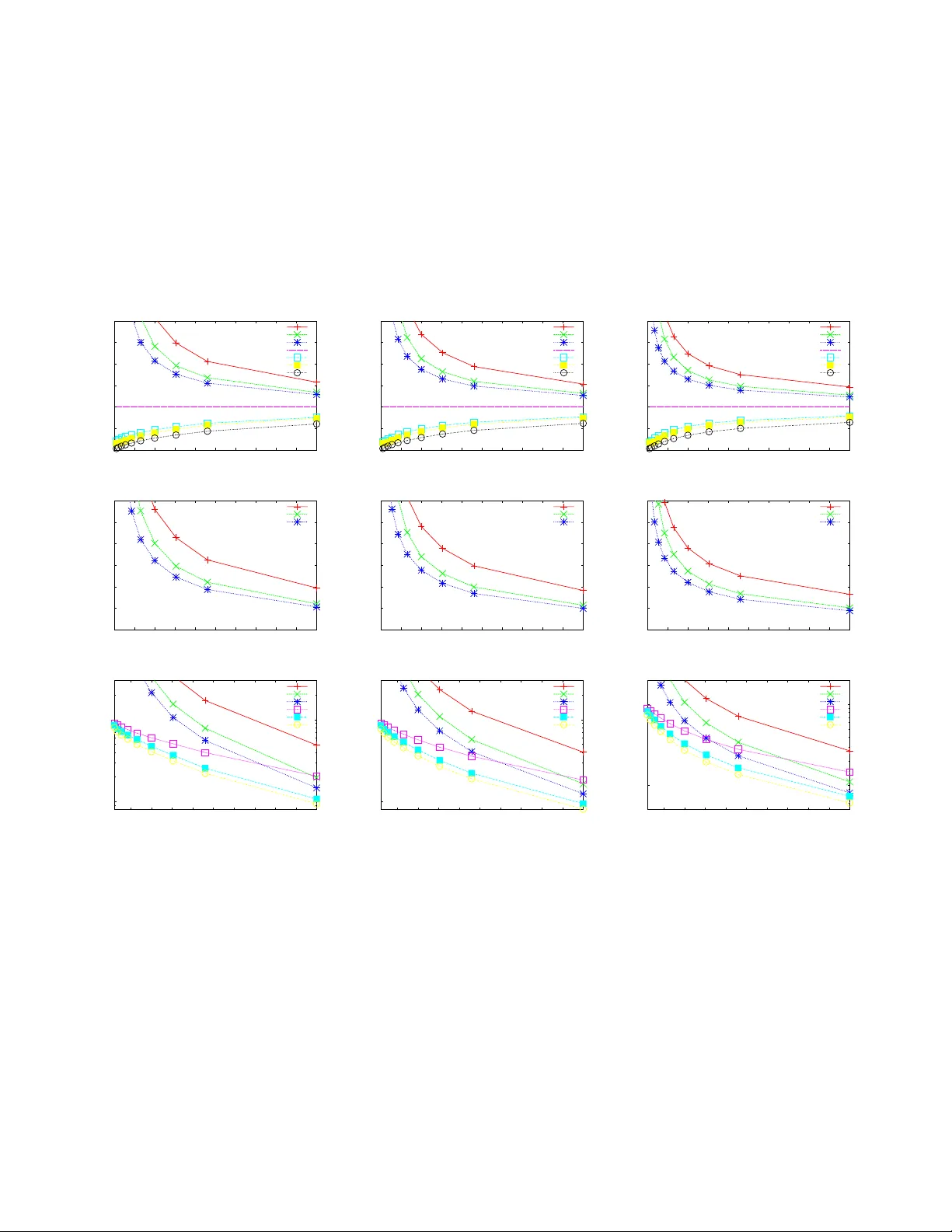
Sketch-Based Estimation of Sub population-W eight Edith Cohen A T&T Labs–Research 180 P ar k A v enue Florham P ar k, NJ 07932, USA edith@resea rch.att.com Haim Kaplan School of Computer Science T el A viv Univ ersity T el A viv , Israel haimk@cs.tau.ac.il ABSTRA CT Summaries of massiv e data s ets support approximate query processing o ver the original data. A basic agg regate o ver a set of records is the w eight of subp opulations speciﬁed as a predicate o ver records’ attributes. Bottom- k sketc hes are a p o w erful summarization forma t of weigh ted items that includes priorit y sampling [18] ( pri ) and the cla ssic w eigh ted sampling without replacement ( ws ). They can b e computed eﬃcien tly for many represen tations of the d ata including distributed databases and data streams. W e derive no vel un biased estimators and eﬃci ent conﬁ- dence b ounds for subp opulation weigh t. Our estimators and b ounds are ta ilored by distinguishing betw een applications (such as data streams) where the total wei ght of the sketc hed set can be computed by the summarization algorithm with- out a signiﬁcant use of add itional resources, and applications (such as sk etc hes of net w ork neigh borho ods) where this is not the case. Ou r r ank c onditioning ( RC ) estimator, is ap- plicable when the total weigh t is not pro vided. This estima- tor generalizes th e known estimator for pri sketc hes [18] and its deriv ation is simpler. When the total w eigh t is av ailable w e suggest another estimator, th e subset c onditioning ( SC ) estimator which is tighter. Our rigorous deriv ations, based on clever applications of the Horvitz-Thompson estimator (that is not directly ap- plicable to b ottom- k sketches), are complemented by eﬃ- cien t computational metho ds. Performance eval uation using a range of Pareto weigh t distributions d emonstrate consid- erable b eneﬁt s of the ws SC estimator on larger subp opu- lations (ov er all other estimators); of t he ws RC estimator (o ver existing estimators for t his basic sampling metho d); and of our conﬁdence b ounds (ove r all previous app roac hes). Overall , we signiﬁcan tly adv ance th e state-of-the- art estima- tion of subp opulation w eigh t q ueries. 1. INTR ODUCTION Sketc hes or statistical summaries of massiv e data sets are an extremely useful tool. S ketc h es are obtained by app ly- ing a probabilistic summarization algorithm t o the data set. Permission to make dig ital or hard copies of all or part of thi s work for personal or classroom use is granted without fee provi ded that copies are not made or distribut ed for proﬁt or commercial adv antage and that copies bear this notic e and the full citati on on the ﬁrst page. T o cop y otherwise, to republi sh, to post on serve rs or to redistrib ute to lists, requir es prior speciﬁc permission and/or a fee. ACM SI GMOD ’08 V anc ouve r , BC, Canada Copyri ght 200X A CM X-XXXXX-XX-X/XX/XX ... $ 5.00. The algorithm retu rns a sketc h th at has smaller size than the original data set bu t supp orts appro ximate qu ery pro- cessing on the original data set. Consider a set of records I with associates weigh ts w ( i ) for i ∈ I . A basic aggregate ov er such sets is subp opula- tion weight . A subp opulation weight query sp eciﬁes a sub- p opulation J ⊂ I as a p redicate on attribu tes v alues of records in I . The result of the query is w ( J ), th e sum of the weig hts of records in J . This aggregate can b e used to estimate other aggregates over subp opulations such as se- lectivit y ( w ( J ) /w ( I )), and va riance and higher moments of { w ( i ) | i ∈ J } [10]. As an example consider a set of all IP ﬂows going th rough a router or a netw ork d uring some time p erio d. Flo w records conta ining this information are collected at IP routers by tools such as Cisco’s NetFlow [25] (now emerging as an IETF standard). Each ﬂow record contains the num ber of pack et s and bytes in eac h ﬂow. Possi ble sub popu lation queries in this example are numerous. Some examples are “the band- width used for an application such as p2p or W eb traﬃc” or “the band width destined to a sp eciﬁed Autonomous S ys- tem.” The ability to answer such queries is critical for net- w ork management and monitoring, and for anomaly det ec- tion. Another example is census database that includes a record for each households with ass ociated weigh t equal to the household income. Ex ample q ueries are to ﬁnd t otal income by region or by the gender of th e head of the household. T o supp ort subp opulation selection with arbitrary p redi- cates, the summary must retain content of some ind ividual records. Two common summarization metho ds are k -mins and b ott om- k sketc hes. Bo ttom- k sketches are obtained by assigning a r ank value , r ( i ), for each i ∈ I that is indep en- dently drawn from a distribution that dep ends on w ( i ) ≥ 0. The b ottom- k sketch con tains the k records with smallest rank v alues [7, 24]. The distribution of th e ske tches is de- termined by the family of d istributions th at is used to draw the rank v alues: By appropriately selecting this family , we can obtain sketc h es that are distributed as if we dra w records without replacement with probability prop ortional to their w eigh ts ( ws ), which is a classic sampling metho d with a sp ecial structure that allo ws sketc hes to be computed more eﬃcien tly than other b ottom- k ske tches. A diﬀerent selec- tion corresp onds to the recently prop osed priority sketches ( pri ) [18, 1], whic h h a v e estimators that minimize the sum of p er-record v ariances [30]. k -mins sk etc hes [7] are obtained by assigning indep endent random rank s to records (again, the distribution used for each record d epend s on the wei ght 1 of the record). The record of smallest rank is selected, and this is rep eated k times, u sing k indep en dent rank assign- ments. k -mins sketc hes include weig hted sampling with re- placemen t ( wsr ). Bottom- k ske tches are more informative than resp ective k -mins sketches ( ws b ottom- k sketc hes can mimic wsr k -mins sketches [14]) and in most cases can b e derived m uc h more eﬃciently . Before delving into the focus of th is pap er, whic h is es- timators and conﬁdence b ounds for subp opulation wei ght, w e o verview classes of applications where these ske tches are prod uced, and which b eneﬁt from our results. Bottom- k and k -mins sketc hes are used as summaries of a single weigh ted set or as summaries of multiple subsets that are d eﬁned ov er the same ground set. In the latter case, the sketches of diﬀerent subsets are “coordinated” in the sense that each record obtains a consistent rank v alue across all t h e subsets it is included in. These coordinated sketc h es supp ort subp opulation selection b ased on subsets’ memberships (such as set u n ion and intersection). W e distinguish b etw een explicit or impli cit representa- tions of the data [14]. Explicit representations list th e o ccur- rence of each record in each subset. They include a rep re- senta tion of a single weigh ted set (for ex ample, a distributed data set or a data stream [15, 1]) or when there are multi- ple su b sets that are represented as item- su bset pairs ( for example, item-basket associations in a market basket data, links in w eb pages, features in do cuments [5, 3, 24, 29, 2]). Bottom- k sketc hes can b e compu t ed muc h more eﬃcien tly than k -mins ske tches when the data is represented explic- itly [4, 24, 12, 14]).). Implicit representations are t hose where t h e multiple sub- sets are sp eciﬁed compactly and implicitly (for example, as neighborho ods in a metric space [7, 16 , 15, 23, 22 , 13].) In these applications, th e summarization algorithm is ap- plied to the compact representation. Beyond comp u tation issues, the distinction b etw een data representations is also imp ortant for estimation: I n applications with exp licit rep- resen tation, th e summarization algorithm can p ro vide the total weig ht of the records without a signiﬁcan t p ro cessing or communication ov erhead. In applications with implic- itly represented data, and for sketc hes computed for subset relations, th e total w eigh t is not readily av ailable. An imp ortan t var ian t uses hash v alues of the identiﬁers of the records instead of random rank s. F or k -mins sketc hes, families of min-wise indep endent hash functions or ǫ -min- wise functions hav e the desirable prop erties [5, 6, 17]. H ash- ing had also b een used with bottom- k sketc hes [4, 24, 2]. This v ariant h as the prop ert y that all copies of the same record obtain th e same rank v alue across subsets without the need for coordination b et w een copies or add itional b o ok keeping. Therefore hashing allo ws to p erform aggregations o ver distinct o c curr enc es (see [19]). F or records associated with p oin ts in some metric space such as a graph, the Euclidean plane, a netw ork, or th e time axis (data streams) [7, 11, 22], ske tches are pro duced for neighborho ods of locations of interest. F or example, all records that lie within some d istance from a lo cation or hap- p ened within some elapsed time from t he current time. F or such metric applications, w e do not wan t to explicitly store a separate sketc h for each p ossible d istance. This is ad - dressed by al l-distanc es sketches . The all-distances sketch of a lo cation is a succinct representation of th e sketc hes of neighborho ods of all distances from the location. A ll- distances k -mins sketc h were in trod uced in [7, 11]. All- distances b ottom- k sketc hes were p roposed and analyzed in [14]. All-distances ske tches also supp ort sp atial ly or tem- p or al ly de c aying aggr e gation [22, 11]. One application of deca ying aggregates is kernel density estimators [27] and typicali ty estimation [21 ] – The estimated d en sit y is a lin- ear combination of the sub popu lation w eigh t o v er neighbor- hoo ds. Overview. Section 2 contains some bac kground and deﬁ- nitions. In S ection 3 we apply th e Maximum Likelihood principle to derive ws ML estimators. These estimators are applicable to ws sketc hes as our deriv ation exp loits sp ecial prop erties of the exp onential distribution used to pro d uce these sketc hes. Wh ile biased, ws M L estimators can b e computed eﬃciently and p erform well in practice. Section 4 introduces a v arian t of the Horvitz-Thompson ( HT ) estimator [20]. The HT estimators assign a p osi- tive adjuste d weight to eac h record t hat is included in the sketc h . Records not includ ed in the sk etc h ha ve zero ad- justed weigh t. The adjusted weig ht has t h e prop erty that for eac h record, th e exp ectation of its adjusted w eigh t ov er sketc h es is equal t o its actual we igh t. The adjusted w eigh t is therefore an unbiase d estimator of the w eight of the record. F rom linearit y of exp ectation, the sum of the adjusted weig hts of records in th e sketch that are members of a su bp opula- tion constitutes an u nbia sed estimate of the weigh t of th e subp opulation. The HT estimator assigns to each included record an ad- justed weigh t equal t o its actual weig ht divided by the p rob- abilit y that it is includ ed in a sketc h. This estimator mini- mizes the p er-record v aria nce of the adjusted w eigh t for th e particular distribu t ion ov er sketc hes. The HT estimator, how ever, cannot b e compu ted for b ottom- k sketc hes, since the probab ility that a record is includ ed in a sketc h cannot b e determined from the information av ailable in the sk etc h alone [26, 28]. Our v arian t, which we refer to as HT on a p artitione d sample sp ac e ( HT p ), ov ercomes this hurdle by applying the HT estimator on a set of partitions of the sam- ple space such that th is probablity can be compu t ed in each subspace. W e apply HTp to derive R ank Conditioning estimators ( RC ) for general b ottom- k sk etches (th at is, sketches pro- duced with arbitr ary families of rank distribut ions). Our deriv ation genera lizes and simpliﬁes one for pri sketc hes ( pri RC estimator) [18] and revea ls general principles. It provides tighter and simpler estimators for ws sketc hes than previously kn o wn. W e show that the cov ariance b et w een ad- justed wei ghts of diﬀerent records is zero and therefore the v aria nce of t h e sub pop u lation weigh t estimator is equ al to the sum of the v ariances of the records. In Section 5 we again apply HTp and derive subset c on- ditioning estimators for ws sketches ( ws SC ). These esti- mators use th e total weig ht w ( I ) in the compu t ation of the adjusted weigh ts. The ws SC estimator is su p erior t o the ws RC estimator, with lo w er v ariance on any subp opulation: The v ariance for each record is at most that of th e ws RC estimator, cov ariances of diﬀerent records are ne gative , and the sum of all co v ariances is zero. These prop erties give the ws SC estimator a distinct adv antage as the relative vari - ance decreases for larger subp opulations. The S C deriv ation exploits special prop erties of ws sketc hes – there is no known pri estimator with negative co v ariances. Moreov er, the ws SC estimator is strictly b etter than any wsr estimator: it 2 has a low er sum of p er-record v ariances than the HT wsr estimator (that minimizes the sum of per- record v ariances for wsr bu t cov ariances do not cancel out) and is also b et- ter t han th e wsr “ratio” estimator b ased on the sum of multipli cities in the sample of records that are members of the subp opulation (whic h do es has n egativ e cov ariances that cancel out but a m uch higher sum of p er-record v ariances on skew ed distributions). The ws SC estimator is expressed as a deﬁn ite integral. W e provide an eﬃcient approximation metho d that is based on a Marko v chain that conv erges to this estimator. After any ﬁxed number of steps of the Marko v c hain we get an unbiased estimate th at is at least as goo d as ws RC . W e implemented and compared the p erformance of a k -mins estimator ( wsr ), ws ML , pri RC , ws RC , and th e approxi- mate ws SC estimators on Pa reto weigh t distributions with a range of skew parameters (see Section 7). When the total w eigh t is unknown or is n ot used, the p erformances of ws ML , ws RC , and p ri RC are almost indistinguishable. They outp erform wsr and the p erformance gain gro ws with the skew of th e data. Therefore, our estimator for ws sketc h es nearly matc h the b est estimators on an optimal sketc h dis- tribution. When the total wei ght is provided, t h e ws SC es tima- tor has a signiﬁcant advan tage (smaller v ariance) on larger subp opulations and emerges as th e b est estimator. The sim- ulations also sho w that the app ro ximate ws SC estimator is very eﬀectiv e even with a small number of steps. Conﬁdence interv als are critical for many applications. In Section 6 we derive conﬁd ence interv als (tailored to appli- cations where the total weigh t is or is n ot pro vided) and develop methods to eﬃciently compute these b ounds. In Section 7 we compare our conﬁdence b ounds with p revious approac hes (a b ound for pri sketc hes [31] and known wsr estimators) using a range of Pareto d istributions with dif- feren t skew parameters. O ur b ounds for ws sk etc hes are signiﬁcan tly tighter than the p ri bounds, ev en when t he total we igh t is not used. This may seem surprising since com bined with our results, the pri RC estimator h as nearly optimal v ariance [30] among all RC estimators. The ex pla- nation is th at th e conﬁdence interv als do not reﬂect this near optimalit y . Our ws conﬁdence b ounds deriva tion, based on some sp ecial properties of ws sk etches, exploits t he in for- mation av ailable in the sketc h. W e p oint on the sources of slac k in the pri conﬁ dence b ounds of [31] that explain its inferior b eha vior. W e prop ose app roaches to add ress some non-inherent sources of slack. Ou r ws b ounds that use the total w eigh t are tighter, in particular for large subp opula- tions, th an those that do not use the total weig ht. A short summary of some of the results in this pap er ap- p eared in [12]. 2. PRELIMIN ARIES Let ( I , w ) be a w eigh ted set. A r ank assignment maps eac h item i t o a random rank r ( i ). The rank s of items are drawn indep endently using a family of distributions f w ( w ≥ 0), where the rank of an item with weig ht w ( i ) is draw n from f w ( i ) . F or a subset J of items and a rank assignment r () we d eﬁne B i ( r () , J ) to b e th e item in J with i th smallest rank according to r () and r i ( J ) ≡ r ( B i ( r () , J )) to b e the i th smallest rank v alue of an item in J . Definition 2.1. k -mins sketc hes ar e pr o duc e d fr om k in- dep endent r ank assignments, r (1) () , . . . , r ( k ) () . The sketch of a subset J is the k -ve ctor ( r (1) 1 ( J ) , r (2) 1 ( J ) , . . . , r ( k ) 1 ( J )) . F or some applic ations, we use a sketch that includes with e ach entry an i dentiﬁer or some othe r attributes such as the weight of the items B 1 ( r ( j ) () , J ) ( j = 1 , . . . , k ). Definition 2. 2. Bottom- k sketc hes ar e pr o duc e d fr om a single r ank assignment r () . The b ottom- k sketch s ( r () , J ) of the subset J is a list of entries ( r i ( J ) , w ( B i ( r () , J ))) for i = 1 , . . . , k . (If | J | < k then the list c ontains only | J | items.) The list is or der e d by r ank, f r om smal lest to lar gest. In addition to the weight, the sketch may include an iden- tiﬁer and attribute values of items B i ( r () , J ) ( i = 1 , . . . , k ). We also i nclude with the sketch the ( k + 1) st smal lest r ank value r k +1 ( J ) (without additional attributes of the item with this r ank value). In fact, b ottom- k sketches must include the items’ w eigh ts but do n ot need to store all rank v alues and it suﬃces to store r k +1 . Using the w eigh ts of the items with k smallest ranks and r k +1 , w e can r e dr aw rank v alues to items in s u sing th e density function f w ( x ) / F w ( r k + 1 ) for 0 ≤ x ≤ r k +1 and 0 elsewhere, for item with weigh t w [14]. Lemma 2.3 . Thi s pr o c ess of r e-assigning r anks i s e quiv- alent to dr awing a r andom r ank assignment r () and taking s ( r ′ () , J ) fr om the pr ob ability subsp ac e wher e { B 1 ( r ′ () , J ) , . . . , B k ( r ′ () , J ) } = { B 1 ( r () , J ) , . . . , B k ( r () , J ) } (the same subset of items with k smal lest r anks, not ne c es- sarily in the same or der) and r k +1 ( J ) = r ′ k +1 ( J ) . 1 Bottom- k and k -mins sketc hes hav e the follo wing useful prop ert y: The sketch of a union of tw o sets can b e generated from the ske tches of th e tw o sets. Let J, H b e tw o subsets. F or an y rank assignmen t r (), r ( J ∪ H ) = min { r ( J ) , r ( H ) } . Therefore, for k -mins sketc hes we hav e ( r 1 ( J ∪ H ) , . . . , r k ( J ∪ H )) = (min { r 1 ( J ) , r 1 ( H ) } , . . . , min { r k ( J ) , r k ( H ) } ) . This prop erty also holds for b ottom- k sketc hes. The k smallest ranks in the union J ∪ H are contained in the union of the sets of the k - smallest ranks in each of J and H . That is, B k ( r () , J ∪ H ) ⊂ B k ( r () , J ) ∪ B k ( r () , H ). Therefo re, the b ottom- k sketc h of J ∪ H can b e computed by taking the pairs with k smallest ranks in the combined sk etc hes of J and H . T o supp ort subset relation qu eries and subset unions, the sketc h es must preserve all rank v alues. ws sketches. The choice of whic h family of random rank functions to u se matters only when items are w eigh ted. Oth- erwise, we can map (b ijectiv ely) th e ranks of one rank func- tion to ranks of another rank function in a wa y that pre- serve s the b ottom- k sketc h. 2 Rank functions f w with some conv enien t prop erties are exp onential distribut ions with p a- rameter w [7]. The den sit y function of this distribution is f w ( x ) = we − wx , and its cumula tive distribution function is F w ( x ) = 1 − e − wx . The minimum rank r ( J ) = min i ∈ J r ( i ) of an item in a subset J ⊂ I is exp onentially distributed with 1 As we shall see in Section 5.2, if w ( J ) is provided and w e use ws sketc hes, we can redraw all rank v alues, eﬀectively obtaining a rank assignmen t from the probability sub space where the subset of items with k smallest rank s is th e same. 2 W e map r such that F 1 ( r ) = α to r ′ such t hat F 2 ( r ′ ) = α , where F 1 is the CDF of th e ﬁrst rank function an d F 2 is the CDF of the other (assuming the CDFs are contin u ous). 3 parameter w ( J ) = P i ∈ J w ( i ) (the minimum of indep end ent exp onentia lly distributed random v ariables is exp onentially distributed with parameter equ al to the sum of the p arame- ters of these distribut ions). Cohen [7] used this prop erty to obtain unbiased low-v ariance estimator s for b oth the weigh t and th e in vers e w eigh t of the subset. 3 With exp onen tial ranks the item with th e minimum rank r ( J ) is a weighte d r andom sample from J : The probability that an item i ∈ J is the item of minimum rank is w ( i ) /w ( J ). Therefore, a k -mins sketc h of a subset J corresp onds to a w eigh ted random sample of size k , drawn wi th repl ace- ment from J . W e call k -mins sketc h using exp onential ranks a wsr sketch. On the other hand , a b ottom- k sketch of a subset J with exp onentia l ranks corresponds to a w eigh ted k - sample d ra wn without replacement from J [14 ]. W e call such a sketc h a ws sk etc h. The follo wing property of exponentially-distributed rank s is a consequence of the memoryless nature of th e exp onential distribution. Lemma 2.4 . [14] Consider a pr ob ability subsp ac e of r ank assignments over J wher e the k items of smal lest r anks ar e i 1 , . . . , i k in i ncr e asing r ank or der. The r ank diﬀer enc es r 1 ( J ) , r 2 ( J ) − r 1 ( J ) , . . . , r k +1 ( J ) − r k ( J ) ar e indep endent r andom variables, wher e r j ( J ) − r j − 1 ( J ) ( j = 1 , . . . , k + 1 ) is exp onential l y di stribute d with p ar ameter w ( J ) − P j − 1 ℓ =1 w ( i ℓ ) . (we formal l y deﬁne r 0 ( J ) ≡ 0 .) ws sketc hes can b e computed more eﬃcien tly than other b ottom- k sketc hes in some imp ortant settings. One suc h example is unaggregated data (eac h item app ears in multi- ple “pieces”) [9, 8] th at is distributed or resides in ex ternal memory . Computing a b ottom- k sketc h generally requires pr e-aggr e gating th e data, so that w e hav e a list of all items and th eir we igh t, which is a costly operation. A key property of exp onenti al ranks is that w e can obt ain a rank va lue for an item by compu ting i ndep endently a rank v alue for each piece, based on th e weig ht of the piece. The rank v alue of the item is the minimum rank v alue of its p ieces. The ws sketc h contains the items of the k pieces of dis- tinct items with smallest ranks and can b e computed in tw o comm unication round s ov er d istributed data or in t w o lin- ear passes: The ﬁrst pass identiﬁes the k items with smallest rank v alues. The second pass is used to add up the weigh ts of the p ieces of each of these k items. Another example is when items are partitioned su c h that w e h a v e the weigh t of eac h part. In this case, a ws sketc h can b e computed while pro cessing only a fraction of the items. A key prop erty is that th e minimum rank va lue ov er a set of items d ep end s only on the sum of t he wei ghts of th e items. Using this p roperty , we can quickly determine which parts contri bute to the sketch and eliminate chunks of items th at b elong to oth er parts. The same p roperty is also useful when sketc hes are com- puted online ov er a stream. Bottom- k sketc hes are pro duced using a priority queue that maintains the k + 1 items with smallest ranks. W e d ra w a rank for each item and u pd ate the queue if this rank is smaller than the largest rank in the queu e. With ws sketc hes, w e can simply draw d irectly from a distribution the accumulated weigh t of items t hat 3 Estimators for th e inv erse-w eigh t are useful for obtaining unbiased estimates for q u an tities where the we igh t app ears in the denominator suc h as th e weigh t ratio of t w o diﬀerent subsets. can b e “skipp ed” b efore we obtain an item with a smaller rank v alue th an th e largest rank in the queue. The stream algorithm simply adds u p the w eigh t of items until it reac hes one that is incorp orated in the sketc h . pri sketches. With p riority ranks [18, 1] the rank v alue of an item with w eig ht w is selected un iformly at rand om from [0 , 1 /w ]. This is eq u iv alent to choosing a rank v alue r /w , where r ∈ U [0 , 1], t he uniform distribution on the interv al [0 , 1]. It is well known that if r ∈ U [0 , 1] then − ln( r ) /w is an exp onential random v ariable with parameter w . There- fore, in contrast with priority ranks, ex ponential ranks cor- respond to u sing rank v alues − ln r /w where r ∈ U [0 , 1]. pri sketc hes are of interest b ecause one can derive from them an estimator th at (n early) minimizes the sum of p er- item v ariances P i ∈ I v ar ( ˜ w ( i )) [30]. More precisely , S zegedy sho w ed that the sum of p er-item v ariances using pri sketc hes of size k is no larger than th e smallest sum of v ariances attainable by an estimator that uses sketc hes with av erage size k − 1. 4 Some of our results apply t o arbitrary rank functions. S ome basic properties that hold for b oth pr i and ws ranks are monotonicity – if w 1 ≥ w 2 then for all x ≥ 0, F w 1 ( x ) ≤ F w 2 ( x ) (items with larger weigh t are more likely to ha ve smaller ranks) and i nvariability to sc aling – scaling of all the w eigh ts does not change the d istribution of subsets selected to the sketc h. Review of weight estimators for wsr sketches. F or a sub- set J , th e rank v alues in the k -mins sketch r 1 ( J ) , . . . , r k ( J ) are k in d epend en t samples from an ex ponential distribu- tion with parameter w ( J ). The quantit y k − 1 P k h =1 r h ( J ) is an unbiased estimato r of w ( J ). The standard deviation of this estimator is equ al to w ( J ) / √ k − 2 and th e av erage (absolute v alue of the) relative error is approximately p 2 / ( π ( k − 2)) [7]. The quanti ty k P k h =1 r h ( J ) is t h e max im um likelihoo d estima- tor of w ( J ). This estimator is k/ ( k − 1) times th e unbias ed estimator. Hence, it is obviously biased, and t he bias is equal t o w ( J ) / ( k − 1). Since the standard deviation is ab out (1 / √ k ) w ( J ), the bias is not signiﬁcant when k ≫ 1. The quantit y P k h =1 r h ( J ) k is an unbiased estimator of the inverse weight 1 /w ( J ). The standard deviation of th is estimate is 1 / ( √ kw ( J )). Subp opulation weig ht estimators for wsr sketc hes when the total w eigh t is k no wn are th e HT estimator, where the adjusted w eigh t is the ratio of the weigh t of the item and the probabilit y 1 − (1 − w ( i ) /w ( I )) k that it is sampled. This estimator minimizes t h e sum of p er-item v ariances bu t co- v aria nces do not cancel out. Anoth er estimator is the sum of m ultiplicities of items in the ske tch that are members of the subp opulation, multiplied by total weig ht, and divided by k . This estimator h as cov ariances t hat cancel out, but higher p er-item v ariances. With wsr sketc hes it is not p os- sible to obt ain an estimator with minim um sum of p er-item v aria nces and co v ariances t hat cancel out. 3. MAXIMUM LIKELIHOOD ESTIMA TORS FOR WS SKETCHES 4 Szegedy’s pro of applies only to estimators based on ad- justed wei ght assignments. It also does not app ly to estima- tors on t he w eigh t of su bp op u lations. 4 Estimating the total weight. Consider a set I and its b ottom- k ske tch s . Let i 1 , i 2 , . . . , i k b e the items in s or- dered by increasing rank s (we use the notation r ( i k +1 ) for the ( k + 1)st smallest rank). If | I | ≤ k (and w e can determine this) then w ( I ) = P w ( i j ). Consider the rank diﬀerences, r ( i 1 ) , r ( i 2 ) − r ( i 1 ) , . . . , r ( i k +1 ) − r ( i k ). F rom Lemma 2.4, they are in d epend en t exp onentially distributed random v ariables. The join t probability densit y function of this set of diﬀerences is therefore the pro duct of the den sit y functions w ( I ) exp( − w ( I ) r ( i 1 ))( w ( I ) − s 1 ) exp( − ( w ( I ) − s 1 )( r ( i 2 ) − r ( i 1 ))) · · · where s ℓ = P ℓ j =1 w ( i j ). Think abou t this probability den- sit y as a function of w ( I ). The maximum likelihoo d estimate for w ( I ) is the v alue that max imizes this fun ction. T o ﬁnd the maximum, take the natural logarithm (for simpliﬁca- tion) of t he expression and look at t he v alue which makes the deriv ative zero. W e obtain th at the maximum likelihoo d estimator ˜ w ( I ) is the solution of the equation k X i =0 1 ˜ w ( I ) − s i = r ( i k +1 ) . (1) The left h and side is a monotone function, and the equ a- tion can b e solved by a b inary searc h on the range [ s k + 1 /r ( i k +1 ) , s k + ( k + 1) /r ( i k +1 )]. W e can obtain a tighter estimator (smaller v ariance) by redrawing the rank v alues of the items i 1 , . . . , i k (see Lemma 2.3) and t aking the exp ec- tation of the solution of Eq. (1) (or a v erage o ver multiple draw s). Estimating a subpop ulation weight. W e derive maxim um lik elihoo d subp opulation w eigh t estimators that u se and do not use the total weig ht w ( I ). Let J ⊂ I b e a subp opu- lation. Let j 1 , . . . , j a b e the items in s that are in I \ J . 5 Let r ′ 1 , . . . , r ′ a b e their respective rank v alues and let s ′ i = P h ≤ i w ( j h ) ( i = 1 , . . . , a ). Deﬁne s ′ 0 ≡ 0. Let i 1 , i 2 , . . . , i c b e the items in J ∩ s . Let r 1 , . . . , r c b e their resp ective rank v alues and let s i = P h ≤ i w ( i h ) ( i = 1 , . . . , c ). Deﬁ ne s 0 ≡ 0. ws ML s ubp opulation weight estimator that does not use w ( I ) : Consider rank assignmen ts su c h that rank v alues in I \ J are ﬁx ed and th e order of ranks of the items in J is ﬁxed. The p robabilit y density of th e observed ranks of the ﬁrst k items in J is th at of seeing the same rank d iﬀerences (probability density is ( w ( J ) − s i ) exp( − ( w ( J ) − s i )( r i +1 − r i ) for t he i th diﬀerence) and of the rank diﬀerence b etw een the c + 1 and c smallest ranks in J b eing at least τ − r c (where τ is th e ( k + 1)st smallest rank in the ske tch), whic h is exp( − ( w ( J ) − s c )( τ − r c )). Rank diﬀerences are ind epen d en t, and therefore, th e probabilit y density as a function of w ( J ) is the pro duct of the ab ov e d ensities. The maxim um likel ihoo d estimator for w ( J ) is the v alue th at maximizes th is probabil- it y . If c = 0, the expression exp( − w ( J ) τ ) is maximized for w ( J ) = 0. Otherwise, by taking the n atural logarithm and deriving w e ﬁnd th at the v alue of w ( J ) that maximizes th e probabilit y density is th e solution of P c − 1 h =0 1 ˜ w ( J ) − s h = τ . As with t he estimator of the total w eigh t, we can obtain a tighter estimator by redra wing the rank v alues. ws ML subp opulation w eigh t estimator that uses w ( I ) : W e compute the prob ab ility density , as a fun ction 5 W e assume that using meta attributes of items in th e ske tch w e can d ecide which among them are in J . of w ( J ), of the even t that we obtain the sk etch s with these ranks given that th e p reﬁx of sampled items from I \ J is j 1 , . . . , j a and th e preﬁx of sampled items from J is i 1 , . . . , i c . W e take the n atural logarithms of the joint p robabilit y den- sit y and derive with resp ect to w ( J ). If c = 0, the deriv a- tive is p ositiv e and the probability density is maximized for w ( J ) = 0. If a = 0, th e deriv ative is negative and the prob- abilit y density is maximized for w ( J ) = w ( I ). Otherwise, if a > 0 and c > 0, the p robabilit y d ensit y is maximized for ˜ w ( J ) that is the solution of c − 1 X h =0 1 ˜ w ( J ) − s h − a − 1 X h =0 1 ( w ( I ) − ˜ w ( J )) − s ′ h = 0 . The eq uation is easy to solv e n umerically , b ecause the left hand side is a monotone d ecreasing function of w ( J ). 4. ADJUSTED WEIGHTS Definition 4. 1. A djuste d-weight summarization ( A W S ) of a weighte d set ( I , w ) is a pr ob ability distribution Ω over weighte d sets b of the form b = ( J, a ) wher e J ⊂ I and a is a weight function on J , such that for al l i ∈ I , E ( a ( i )) = w ( i ) . (T o c ompute this exp e ctat ion we extend the weight function fr om J to I by assigning a ( i ) = 0 for items i ∈ I \ J .) F or i ∈ J we c al l a ( i ) the adjuste d w ei ght of i in b . An A WS al gorithm is a p robabilistic algorithm th at in- puts a weigh t ed set ( I , w ) and returns a wei gh ted set ac- cording to some A WS of ( I , w ). An A WS algorithm for ( I , w ) p rovides u nbia sed estimators for the weig ht of I and for the w eigh t of su bsets of I : By linearit y of ex pectation, for any H ⊆ I , the sum P i ∈ H a ( i ) is an unbias ed estimator of w ( H ). 6 Let Ω b e a d istribu tion o ver sketc hes s , where eac h sketc h consists of a subset of I and some add itional information such as the rank v alues of the items included in the subset. Supp ose that give n the sampled sketc h s w e can compute Pr { i ∈ s | s ∈ Ω } for all i ∈ s (since I is a ﬁ n ite set, these probabilities are strictly p ositiv e for all i ∈ s ). Then w e can make Ω into an A W S u sing th e H orvitz-Thompson ( H T ) estimator [20] which provides for eac h i ∈ s the adjusted w eigh t a ( i ) = w ( i ) Pr { i ∈ s | s ∈ Ω } . It is wel l known and easy to see that these ad justed weigh ts are unbiased and have minimal va riance for e ach item for the particular distribution Ω o v er subsets. HT on a partitioned sample space ( HTp ) is a method to derive adjusted we igh ts when w e cann ot d et ermine Pr { i ∈ s | s ∈ Ω } from the sketc h s alone. F or example if Ω is a distribu t ion of b ottom- k sketc hes, then the p robabilit y Pr { i ∈ s | s ∈ Ω } generally dep ends on all th e weigh ts w ( i ) for i ∈ I and t h erefore, it cann ot b e determined from t he information contained in s alone. F or eac h item i we partition Ω into subsets P i 1 , P i 2 . . . . This partition satisﬁes the follo wing t w o requirements 6 A useful prop ert y of adjusted w eigh ts is that th ey pro vide unbiased aggregations ov er any other numeric attribute : F or w eigh ts h ( i ), P i ∈ H h ( i ) a ( i ) /w ( i ) is an u n biased estimator of h ( J ). 5 1. Given a sketc h s , we can determine the set P i j conta in- ing s . 2. F or every set P i j w e can compu te the conditional prob- abilit y p i j = Pr { i ∈ s | s ∈ P i j } . F or each i ∈ s , w e identify the set P i j and use the adjusted w eigh t a ( i ) = w ( i ) /p i j (whic h is the HT adjusted wei ght in P i j ). 7 Items i 6∈ s get an adjusted w eigh t of 0. The exp ected adjusted weigh t of each item i within each subspace of the partition is w ( i ) and therefore its exp ected adjusted weigh t o ver Ω is w ( i ). Rank Conditioning ( RC ) adjusted weigh ts for b ott om- k sketc hes are an HTp estimator. The probability space Ω includes all rank assignments. The sketc h includes the k items with smallest rank val ues and the ( k + 1)st smallest rank r k +1 . The p artition P i 1 , . . . , P i ℓ whic h we use is based on r ank c onditioning . F or each p ossible rank v alue r w e hav e a set P i r conta ining all rank assignments in which the k th rank assigned t o an item other than i is r . (If i ∈ s then this is th e ( k + 1)st smallest rank.) The probability that i is in clud ed in a bottom- k sketc h giv en th at the rank assignmen t is from P i r is the probabilit y that its rank v alue is smaller than r . F or ws sketc h es, this probabilit y is equal to 1 − exp( − w ( i ) r ) . Assume s contai ns i 1 , . . . , i k and that the ( k + 1)st smallest rank r k +1 is known. Then for item i j , the rank assignment b elongs to P i j r k +1 , and therefore th e adjusted weigh t of i j is w ( i j ) 1 − exp( − w ( i j ) r k +1 ) . The ws RC estimator on the total w eigh t is P k j =1 w ( i j ) 1 − exp( − w ( i j ) r k +1 ) . The pri RC adjusted wei ght for an item i j (obtained by a tailored deriv ation in [1]), is max { w ( i j ) , 1 /r k +1 } . V arianc e of RC adjusted weights Lemma 4.2 . Consider RC adjuste d weights and two i tems i , j . Then, cov ( a ( i ) , a ( j )) = 0 (The c ovarianc e of the ad- juste d weight of i and the adjuste d wei ght of j i s zer o.) Pr oof. It suﬃces t o sho w that E ( a ( i ) a ( j )) = w ( i ) w ( j ). Consider a partition of the sample space of all rank assign- ments according to the ( k − 1)th smallest rank of an item in I \ { i, j } . 8 Consider a subset in the partition and let r k − 1 denote the v alue of the ( k − 1)th smallest ran k of an item in I \ { i, j } for rank assignments in this subset. W e show that in this subset E ( a ( i ) a ( j )) = w ( i ) w ( j ). The pro duct a ( i ) a ( j ) is p ositive in this sub set only when r ( i ) < r k − 1 and r ( j ) < r k − 1 , which (since rank assignmen ts are indep endent) happ ens with probab ility p r { r ( i ) < r k − 1 } pr { r ( j ) < r k − 1 } . In this case the k th smallest rank in I \ { i } and I \ { j } is r k − 1 and therefore, a ( i ) = w ( i ) pr { r ( i ) 0 in c is equal to f ( c ∪ { i, j } , ℓ ). Therefore, the conditional p robabilit y is f ( c ∪{ i,j } ,ℓ ) f ( c,ℓ ) . In this case, the ad - justed weigh t assigned to i is set according to items c ∪ { j } having th e ( k − 1) smallest rank s in I \ i . Therefore, this w eigh t is a ( i ) = w ( i ) f ( c ∪ { j } , ℓ ) f ( c ∪ { i, j } , ℓ ) . Symmetrically for j , a ( j ) = w ( j ) f ( c ∪ { i } , ℓ ) f ( c ∪ { i, j } , ℓ ) . W e th erefore obtain that E ( a ( i ) a ( j )) conditioned on this part is w ( i ) w ( j ) f ( c ∪ { j } , ℓ ) f ( c ∪ { i } , ℓ ) f ( c ∪ { i, j } , ℓ ) f ( c, ℓ ) . It suﬃces to sho w th at f ( c ∪ { j } , ℓ ) f ( c ∪ { i } , ℓ ) f ( c ∪ { i, j } , ℓ ) f ( c, ℓ ) ≤ 1 . T o show that, we apply Eq . 3 and substitut e in th e numer- ator f ( c ∪ { j } , ℓ ) = f ( c, ℓ ) − f ( c, ℓ + w ( j ) ) ℓ ℓ + w ( j ) and in t h e denominator f ( c ∪ { i, j } , ℓ ) = f ( c ∪ { i } , ℓ ) − f ( c ∪ { i } , ℓ + w ( j )) ℓ ℓ + w ( j ) The numerator b eing at m ost the denominator t h erefore fol- lo ws from the immediate in eq ualit y f ( c, ℓ ) f ( c ∪ { i } , ℓ + w ( j )) ≤ f ( c, ℓ + w ( j ) ) f ( c ∪ { i } , ℓ ) . Lemma 5.3 . Consider ws sketches of a weighte d set ( I , w ) and subp opulation J ⊂ I . The S C estimator for the weight of J has smal ler varianc e than the RC est imator for the weight of J . Pr oof. By Lemma 4.2 the v aria nce of t he RC estimato r for J is P j ∈ J v ar RC ( a ( j )). So using Lemma 4.4 we obtain that P j ∈ J v ar SC ( a ( j )) is n o larger than th e v ariance of the RC estimator for J . Finally since v ar SC ( X j ∈ J a ( j )) = X j ∈ J v ar SC ( a ( j ))+ X i 6 = j,i,j ∈ J cov SC ( a ( i ) , a ( j )) , and Lemma 5.2 that implies that th e second term is negative the lemma follo ws. 5.3 Computing SC adjusted weights. The adjusted w eigh ts can b e computed by numerical inte- gration. W e p ropose (and implement) an alternative meth od based on a Marko v chain that is faster and easier to imple- ment. The metho d conv erges to the subset conditioning adjusted w eigh ts as the num ber of steps grows . It can b e used with a ﬁxed num ber of steps and p ro vides unbias ed adjusted weigh ts. As an intermediate step w e deﬁne a new estimator as fol- lo ws. W e partition the rank assignments into subspaces, eac h consisting of all rank assignments with the same or- dered set of k items of smallest ranks. Let P b e a subsp ace in the partition. F or each rank assignment in P and item i the adjusted weig ht of i is the exp ectation of the RC ad- justed weigh t of i ov er all rank assignmen ts in P . 9 These adjusted weigh ts are unbiased b ecause t he un derly- ing RC adjusted w eigh ts are unbiased. By th e conv exit y of the v ariance, they ha ve smaller p er-item v ariance than RC . It is also easy to see that the va riance of this estimato r is higher th an the v aria nce of the preﬁx conditioning estima- tor: Rank assignments with the same p reﬁx of items from I \ i , bu t where t he item i app ears in diﬀerent positions in the k -preﬁx, can hav e diﬀerent adjusted weigh ts with th is assignmen t, whereas they h ave th e same adjusted weigh t with preﬁx conditioning. The distribution of r k +1 in each subspace P is th e sum of k indep endent exp onential random v ariables with parameters w ( I ), w ( I ) − w ( i 1 ),. . . , w ( I ) − P k h =1 w ( i h ) where i 1 , . . . , i k are the items of k smallest ranks in rank assignments of P (see Lemma 2.4). S o the ad justed w eigh t of i j ( j = 1 , . . . , k ) is a ( i j ) = E ( w ( i j ) / (1 − exp( − w ( i j ) r k +1 ))) where the expec- tation is ov er this distribution of r k +1 . Instead of compu ting the ex pectation, w e av erag e the R C adjusted weigh ts w ( i j ) / (1 − exp( − w ( i j ) r k +1 )) ov er multiple draw s of r k +1 . This av erage is clearly an unbiased estimator of w ( i j ) and its vari ance decreases with t he num ber of draws. Eac h rep etition can b e implemented in O ( k ) time (drawing and summing k random va riables.). W e deﬁne a Marko v c hain ov er p ermutations of the k items { i 1 , . . . , i k } . Starting with a p erm utation π w e contin ue to a p erm utation π ′ by applying the follow ing p rocess. W e draw r k +1 as d escribed abov e from the distribution of r k +1 in th e subspace correspon d ing to π . W e then redraw rank va lues for the items { i 1 , . . . , i k } as d escribed in Section 2 follo wing Deﬁnition 2.2. The p ermutation π ′ is obtained by reordering { i 1 , . . . , i k } according to the new rank v alues. This Marko v chai n has the follo wing prop erty . Lemma 5.4 . L et P b e a (unor der e d) set of k items. L et p π b e the c onditional pr ob ability that in a r andom r ank as- signment whose pr eﬁx c onsists of items of P , the or der of these items in the pr eﬁx i s as i n π . Then p π is the stationary distribution of the Markov chain describ e d ab ove. Pr oof. Supp ose we draw a p erm utation π of the items in P with probability p π and then draw r k +1 as d escribed above. Then this is equiv alen t to draw ing a random rank assignmen t whose preﬁx consists of items in P and taking r k +1 of this assignmen t. Similarly assume w e draw r k +1 as w e just d escrib ed, dra w ranks for items in P , and order P by these ranks. Then this 9 Note that this is not an instance of HTp , we simply a vera ge another estimator in eac h part. 8 is eq u iv alent to draw ing a p ermutation π with p robabilit y p π . Our implementation is contro lled by t w o parameters inpe rm and pe rmnum . inperm is the number of times the rank v alue r k +1 is redrawn for a p ermutation π (at eac h step of the Marko v chain). permnum is t he num ber of steps of the Mark o v chain (num b er of p ermutatio ns in th e sequence). W e start with the p ermutation ( i 1 , . . . , i k ) obtained in the ws sketc h. W e app ly th is Marko v chain to obtain a se- quence of permnum p ermutations of { i 1 , . . . , i k } . F or eac h p erm utation π j , 1 ≤ j ≤ permnum , w e dra w r k +1 from P π j inperm t imes as describ ed ab o ve . F or eac h su c h draw we compute th e RC adjusted w eigh ts for all items. The ﬁn al adjusted wei ght is the a verag e of the RC adjusted weig hts assigned to the item in the permnum ∗ inperm applications of the RC metho d. W e redra w a p ermutation in this Mark o v chain in O ( k log k ) time ( O ( k ) time to redraw k rank v alues and O ( k log k ) to sort). Redrawing r k +1 giv en a p erm utation takes O ( k ) time. Therefore, the total running time is O ( pe rmnum · k log k + inperm · k ). The expectation of the RC adjusted w eigh ts ov er t h e sta- tionary distribut ion is the subset conditioning adjusted w eigh t. An imp ortant p roperty of this pro cess is that if we apply it for a ﬁxe d number of steps, and av erage over a ﬁxed num ber of d raws of r k +1 within each step, we still obtain unbiased estimators. Our experimental section sho ws that these esti- mators p erform very w ell. The sub set conditioning estimator has p o w erful p roper- ties. Unfortunately , it seems sp eciﬁc t o ws sketc h es. U se of subset conditioning requires th at given a weigh ted set ( H , w ) of k − 1 weig hted items, an item i with weigh t w ( i ), and a weigh t ℓ > 0, we can compute the probability that th e b ottom- k sketc h of a set I that includes H , { i } and has total w eigh t ℓ + w ( H ) + w ( i ) contains the items H ∪ { i } . This probabilit y is determined from the distribution of the small- est rank of items with t otal weigh t ℓ . In general, how ev er, this probability dep ends on the w eigh t distribution of the items in I \ { H ∪ { i }} . The exponential d istribution has the prop ert y that the d istribu t ion of the smallest rank depen d s only on ℓ and not on the weigh t distribution. 6. CONFIDENCE BOUNDS Let r b e a rank assignmen t of a w eig hted set Z = ( H , w ). Recall that for H ′ ⊆ H , r ( H ′ ) is the minimum rank of an item in H ′ . In this section it will b e useful to denote by r ( H ′ ) th e maxim um rank of an item in H ′ . W e deﬁne r ( ∅ ) = + ∞ and r ( ∅ ) = 0. F or a distribution D o v er a totally ordered set (b y ≺ ) and 0 < α < 1, we den ote by Q α ( D ) the α -quantile of D . That is, pr y ∈ D { y ≺ Q α ( D ) } ≤ α and pr y ∈ D { y  Q α ( D ) } ≥ 1 − α . 6.1 T otal weight F or tw o w eigh ted sets Z 1 = ( H 1 , w 1 ) and Z 2 = ( H 2 , w 2 ), let Ω( Z 1 , Z 2 ) b e the probabilit y subspace that contains all rank assignments r ov er Z 1 ∪ Z 2 such t hat r ( H 1 ) < r ( H 2 ). Let ( I , w ) b e a wei ghted set, let r b e a rank assignment for ( I , w ), s b e the b ottom- k sketc h that corresp onds to r (we also u se s as the set of k items with smallest rank s). Let W (( s, w ) , r k +1 , δ ) b e the set containing all w eigh ted sets Z ′ = ( H , w ′ ) such that pr { r ′ ( H ) ≥ r k +1 | r ′ ∈ Ω(( s, w ) , Z ′ ) } ≥ δ . Deﬁne w (( s, w ) , r k +1 , δ ) as follo ws. If W (( s, w ) , r k +1 , δ ) = ∅ , then w ( ( s, w ) , r k +1 , δ ) = 0. Otherwise, let w (( s, w ) , r k +1 , δ ) = sup { w ′ ( H ) | ( H , w ′ ) ∈ W (( s, w ) , r k +1 , δ ) } . (This supremum is w ell deﬁned for “reasonable” families of rank functions, otherwise, we allo w it to b e + ∞ ) Let W (( s, w ) , r k +1 , δ ) b e the set of all weigh ted sets Z ′ = ( H , w ′ ) such that pr { r ′ ( H ) ≤ r k +1 | r ′ ∈ Ω(( s, w ) , Z ′ ) } ≥ δ . Let w (( s, w ) , r k +1 , δ ) b e as follo ws: W e hav e W (( s, w ) , r k +1 , δ ) 6 = ∅ for “reasonable” families of rank functions, but if it is empty , we deﬁ n e w (( s, w ) , r k +1 , δ ) = + ∞ . Otherwise, let w (( s, w ) , r k +1 , δ ) = inf { w ′ ( H ) | ( H , w ′ ) ∈ W (( s , w ) , r k +1 , δ ) } . (This inﬁ m um is well deﬁned since weigh ted sets ha ve n on - negative w eigh t s.) Lemma 6.1 . L et r b e a r ank assignment for the weighte d set ( I , w ) , and let s b e the b ottom- k sketch that c orr esp onds to r Then w ( s ) + w (( s, w ) , r k +1 , δ ) is a ( 1 − δ ) -c onﬁdenc e upp er b ound on w ( I ) , and w ( s ) + w (( s, w ) , r k +1 , δ ) is a (1 − δ ) -c onﬁdenc e l ower b ound on w ( I ) . Pr oof. W e prov e (1). The pro of of (2) is analogous. W e show that in eac h subspace Ω(( s, w ) , ( I \ s, w )) of rank assignmen ts our b ound is correct with probability 1 − δ . Since these subspaces, sp eciﬁed by s ⊂ I of size | s | = k , form a p artition of the rank assignments ov er ( I , w ), the lemma follo ws. Let D k +1 b e the distribution of the ( k + 1)st smallest rank ov er rank assignmen ts in Ω(( s , w ) , ( I \ s , w )) (the small- est rank in I \ s ). Assume that r is a rank assignment in Ω(( s, w ) , ( I \ s, w )) . W e show that if r k +1 ≤ Q 1 − δ ( D k +1 ) then our upp er b ound is correct. Since by the deﬁnition of a quan tile r k +1 ≤ Q 1 − δ ( D k +1 ) with probability ≥ (1 − δ ) in Ω(( s, w ) , ( I \ s , w )), it fol lo ws that our b ound is correct with probabilit y ≥ (1 − δ ) in Ω(( s, w ) , ( I \ s, w )) . If r k +1 ≤ Q 1 − δ ( D k +1 ) then pr { r ′ ( I \ s ) ≥ r k +1 | r ′ ∈ Ω(( s, w ) , ( I \ s, w )) } ≥ pr { r ′ ( I \ s ) ≥ Q 1 − δ ( D k +1 ) | r ′ ∈ Ω(( s, w ) , ( I \ s, w )) } ≥ δ . So w e obtain that ( I \ s, w ) ∈ W (( s, w ) , r k +1 , δ ) and th ere- fore w ( I \ s ) ≤ w ( ( s, w ) , r k +1 , δ ). This lemma also holds for a v ariant, where we consider rank assignments r (and correspond in g subspaces) where the items in s app ear in the same order as in r ′ . 6.2 Subp opulation weight W e derive conﬁden ce b ounds for the w eigh t of a subp op- ulation J ⊂ I . The arguments are more delicate, as th e num ber of items from J th at we see in th e sketc h can v ary b et w een 0 and k and w e do not kn o w if the ( k + 1)th smallest rank b elongs to an item in J or in I \ J . W e wil l work with w eigh ted lists instead of weigh ted sets. A weighte d list ( H , w , π ) consists of a w eigh ted set ( H , w ) and a linear order (p ermutation) π on the elements of H . W e will ﬁnd it con v enient to sometimes sp ecify the permutation π as the order induced by a rank assignment r on H . The c onc atena tion ( H (1) , w (1) , π (1) ) ⊕ ( H (2) , w (2) , π (2) ) of tw o w eigh ted lists, is a we igh ted list with items H (1) ∪ H (2) , correspondin g w eigh ts as deﬁn ed by w ( i ) : H ( i ) and order such that each H ( i ) is ordered according to π ( i ) and the elemen ts of H (1) precede those of H (2) . Let Ω(( H , w , π )) b e the probability su bspace of rank assignmen ts o v er ( H , w ) such t hat the rank order is according to π . Let r b e a rank assignmen t, s b e the corresp onding sketc h, and ℓ b e the weig hted list ℓ = ( J ∩ s, w , r ). Let W ( ℓ, r k +1 , δ ) 9 b e the set of all weig hted lists h = ( H , w ′ , π ) suc h that pr { r ′ ( H ) ≥ r k +1 | r ′ ∈ Ω( ℓ ⊕ h ) } ≥ δ . Let w ( ℓ, r k +1 , δ ) = sup { w ′ ( H ) | ( H , w ′ , π ) ∈ W ( ℓ, r k +1 , δ ) } . (If W ( ℓ, r k +1 , δ ) = ∅ , then w ( ℓ, r k +1 , δ ) = 0. If unboun ded, then w ( ℓ, r k +1 , δ ) = + ∞ .) Let W ( ℓ, r k , δ ) b e the set of all w eigh ted lists h = ( H , w ′ , π ) such that pr { r ′ ( J ∩ s ) ≤ r k | r ′ ∈ Ω( ℓ ⊕ h ) } ≥ δ . Let w ( ℓ, r k , δ ) = inf { w ′ ( H ) | ( H , w ′ , π ) ∈ W ( ℓ, r k , δ ). (If W ( ℓ, r k , δ ) = ∅ , then w ( ℓ, r k , δ ) = + ∞ ). W e prov e the fol- lo wing. Lemma 6.2 . L et r b e a r ank assignment, s b e the c orr e- sp onding sketch, and ℓ b e the weighte d li st ℓ = ( J ∩ s, w, r ) . Then w ( J ∩ s ) + w ( ℓ, r k +1 , δ ) is a (1 − δ ) -c onﬁdenc e up- p er b ound on w ( J ) and w ( J ∩ s ) + w ( ℓ, r k , δ ) is a (1 − δ ) - c onﬁdenc e l ower b ound on w ( J ) . Pr oof. The b ounds are conditioned on th e subspace of rank assignments o ver ( I , w ) where t he ranks of items in I \ J are ﬁxed and the order of the ranks of th e items in J is ﬁxed. These su b spaces are a partition of t he sample space of rank assignmen ts o ver ( I , w ). W e show that the conﬁdence b ounds hold within eac h subsp ace. Consider such a subsp ace Φ ≡ Φ( J, π : J, a : ( I \ J )), where π : J is a p ermutatio n ov er J , representing the order of the ranks of the items in J . and a : ( I \ J ) are the rank v alues of the elements in I \ J . Let D k +1 b e the distribution of r k +1 for r ∈ Φ and let D k b e the distribution of r k for r ∈ Φ. Ov er rank assignments in Φ we hav e pr { r k +1 ≤ Q 1 − δ ( D k +1 ) } ≥ 1 − δ and pr { r k ≥ Q δ ( D k ) } ≥ 1 − δ . 10 W e sho w that • The upp er b ound is correct for rank assignmen ts r ∈ Φ such that r k +1 ≤ Q 1 − δ ( D k +1 ). Therefore, it is correct with probability at least (1 − δ ). • The low er boun d is correct for rank assignmen ts r ∈ Φ such that r k ≥ Q δ ( D k ). Therefore, it is correct with probabilit y at least (1 − δ ). Consider a rank assignment r ∈ Φ. Let s b e the items in the sketc h . Let ℓ = ( J ∩ s, w , r ) and ℓ ( c ) = ( J \ s, w , r ) b e the w eigh ted lists of the items in J ∩ s or J \ s , resp ectively , as ordered by r . There is bijection b etw een rank assignmen ts in Ω( ℓ ⊕ ℓ ( c ) ) and rank assignmen ts in Φ by augmenting the rank assignmen t in Ω( ℓ ⊕ ℓ ( c ) ) with th e ranks a ( j ) for items j ∈ I \ J . F or a rank assignmen t r ∈ Φ let ˆ r ∈ Ω( ℓ ⊕ ℓ ( c ) ) b e its restriction to J . A rank assignmen t r ′ ∈ Φ has r ′ k +1 ≥ r k +1 if and only if b r ′ ( J \ s ) ≥ r k +1 . 11 So if r ∈ Φ such th at r k +1 ≤ Q 1 − δ ( D k +1 ) then pr r ′ ∈ Ω( ℓ ⊕ ℓ ( c ) ) { r ′ ( J \ s ) ≥ r k +1 } = pr r ′ ∈ Φ { r ′ k +1 ≥ r k +1 } ≥ pr r ′ ∈ Φ { r ′ k +1 ≥ Q 1 − δ ( D k +1 ) } ≥ δ . Therefore, ℓ ( c ) ∈ W ( ℓ, r k +1 , δ ), and hence w ( J \ s ) ≤ w ( ℓ, r k +1 , δ ) and th e upp er b ou nds holds. 10 Note that these distributions hav e some discrete v alues with p ositive probabilities, therefore, it does not neces- sarily holds that pr { r k ≤ Q δ ( D k ) } ≤ δ and p r { r k +1 ≥ Q 1 − δ ( D k +1 ) } ≤ δ . 11 Note th at th e statement with strict inequ alities do es not necessarily hold. A rank assignment r ′ ∈ Φ has r ′ k ≤ r k if and only if the maximum rank th at b r ′ giv es to an item in J ∩ s is ≤ r k . So if r ∈ Φ suc h that r k ≥ Q δ ( D k ) pr r ′ ∈ Ω( ℓ ⊕ ℓ ( c ) ) { r ′ ( J ∩ s ) ≤ r k } = pr r ′ ∈ Φ { r ′ k ≤ r k } ≥ pr r ′ ∈ Φ { r ′ k ≤ Q δ ( D k ) } ≥ δ Therefore, ℓ ( c ) ∈ W ( ℓ, r k , δ ), and hence w ( J \ s ) ≥ w ( ℓ , r k , δ ) and the lo w er b ound holds. 6.3 Subp opulation weight using w(I) W e d eriv e tighter conﬁdence interv als that use th e total w eigh t w ( I ). F or w eigh ted lists h ( i ) = ( H ( i ) , w ( i ) , π ( i ) ) ( i = 1 , 2), t he probability space Ω( h (1) , h (2) ) contains all rank as- signmen ts r ov er the w eigh t ed set ( H (1) , w (1) ) ∪ ( H (2) , w (2) ) such that for eac h i = 1 , 2, the order of H ( i ) induced by the rank v alues r : H ( i ) is π ( i ) . W e deﬁ ne the fun ctions c h (1) ,h (2) ( r ) and d h (1) ,h (2) ( r ) for r ∈ Ω( h (1) , h (2) ) as follo ws: c h (1) ,h (2) ( r ) is the number of items amongst those with k smallest ranks th at are in H (1) (equiv alen tly , it is i such that r i ( H (1) ) < r k − i +1 ( H (2) ) and r k − i ( H (2) ) < r i +1 ( H (1) )); d h (1) ,h (2) ( r ) = r k − c h (1) ,h (2) ( r ) ( H (2) ) − r c h (1) ,h (2) ( r ) ( H (1) ) is the diﬀerence b et w een the largest rank v alues of items in H (2) and H (1) that are amongst the k least ranked items. W e use t he notation ( c 1 , d 1 )  ( c 2 , d 2 ) for the lexico- graphic order over pairs. Let r b e a rank assignment, and let s b e the sketc h cor- respond ing to r . Let ∆ = r (( I \ J ) ∩ s ) − r ( J ∩ s ), and let ℓ 1 = ( J ∩ s, w, r : J ∩ s ) and ℓ 2 = (( I \ J ) ∩ s, w, r : ( I \ J ) ∩ s ). Let W ( ℓ 1 , ℓ 2 , ∆ , δ ) b e the set of all pairs ( h 1 , h 2 ) of weig hted lists h 1 = ( H 1 , w 1 , π 1 ) and h 2 = ( H 2 , w 2 , π 2 ) such that w 1 ( H 1 ) + w 2 ( H 2 ) = w ( I ) − w ( s ) and pr { ( c ℓ 1 ⊕ h 1 ,ℓ 2 ⊕ h 2 ( r ′ ) , d ℓ 1 ⊕ h 1 ,ℓ 2 ⊕ h 2 ( r ′ ))  ( | J ∩ s | , ∆) } ≥ δ , (4) o ver th e probabilit y space of all r ′ ∈ Ω( ℓ 1 ⊕ h 1 , ℓ 2 ⊕ h 2 ). If W ( ℓ 1 , ℓ 2 , ∆ , δ ) = ∅ , then w ( ℓ 1 , ℓ 2 , ∆ , δ ) = 0. Otherwise, w ( ℓ 1 , ℓ 2 , ∆ , δ ) = sup { w 1 ( H 1 ) | ( h 1 , h 2 ) ∈ W ( ℓ 1 , ℓ 2 , ∆ , δ ) } . Let W ( ℓ 1 , ℓ 2 , ∆ , δ ) b e the set of all pairs ( h 1 , h 2 ) of weig hted lists h 1 = ( H 1 , w 1 , π 1 ) and h 2 = ( H 2 , w 2 , π 2 ) such that w ( H 1 ) + w ( H 2 ) = w ( I ) − w ( s ) and pr { ( c ℓ 1 ⊕ h 1 ,ℓ 2 ⊕ h 2 ( r ′ ) , d ℓ 1 ⊕ h 1 ,ℓ 2 ⊕ h 2 ( r ′ ))  ( | J ∩ s | , ∆) } ≥ δ , (5) o ver th e probabilit y space of all r ′ ∈ Ω( ℓ 1 ⊕ h 1 , ℓ 2 ⊕ h 2 ). If W ( ℓ 1 , ℓ 2 , ∆ , δ ) = ∅ , then w ( ℓ 1 , ℓ 2 , ∆ , δ ) = w ( I ) − w ( s ). Otherwise, w ( ℓ 1 , ℓ 2 , ∆ , δ ) = inf { w 1 ( H 1 ) | ( h 1 , h 2 ) ∈ W ( ℓ 1 , ℓ 2 , ∆ , δ ) } . Lemma 6.3 . L et r b e a r ank assignment, s b e the c orr e- sp onding sketch, let ∆ = r (( I \ J ) ∩ s ) − r ( J ∩ s ) , and let ℓ 1 = ( J ∩ s , w , r : J ∩ s ) and ℓ 2 = (( I \ J ) ∩ s, w , r : ( I \ J ) ∩ s ) . Then w ( J ∩ s ) + w ( ℓ 1 , ℓ 2 , ∆ , δ ) is a ( 1 − δ ) -c onﬁdenc e upp er b ound on w ( J ) , and w ( J ∩ s ) + w ( ℓ 1 , ℓ 2 , ∆ , δ ) is a (1 − δ ) - c onﬁdenc e l ower b ound on w ( J ) . Pr oof. The lo w er b ound on w ( J ) is equal to w ( I ) mi- nus a (1 − δ )- conﬁdence upp er b ound, w (( I \ J ) ∩ s ) + w ( ℓ 2 , ℓ 1 , − ∆ , δ ) on w ( I \ J ). Therefore it suﬃces to prov e the upp er b ound. W e sh o w that the b ound holds with probability at least (1 − δ ) in the subspace of rank assignments o ver ( I , w ) where the rank order of the items in J and th e rank order of th e items in I \ J are ﬁxed. These subspaces are a partition of 10 the space of rank assignments. Consider suc h a subspace Φ = Ω( ℓ ′ 1 , ℓ ′ 2 ). Let ℓ ′ 1 = ( J, w, π 1 ) and ℓ ′ 2 = ( I \ J, w , π 2 ) b e the wei ghted lists that correspon d s to the rank order of the items in J and in I \ J , respectively , for r ∈ Φ. Let D b e the distribution o ver the pairs ( c ℓ ′ 1 ,ℓ ′ 2 ( r ) , d ℓ ′ 1 ,ℓ ′ 2 ( r )) for r ∈ Φ. W e d eﬁne the quantile Q 1 − δ ( D ) with resp ect to the lexicographic order ov er the pairs. W e show th at the upp er b ound is correct for all r ∈ Φ such that ( c ℓ ′ 1 ,ℓ ′ 2 ( r ) , d ℓ ′ 1 ,ℓ ′ 2 ( r ))  Q 1 − δ ( D ) . Therefor e, it holds with probability at least 1 − δ . Let r ∈ Φ such that ( c ℓ ′ 1 ,ℓ ′ 2 ( r ) , d ℓ ′ 1 ,ℓ ′ 2 ( r ))  Q 1 − δ ( D ) . Let s b e the correspond ing sketc h, ℓ 1 = ( J ∩ s, w, r ), ℓ 2 = (( I \ J ) ∩ s , w , r ), ℓ ( c ) 1 = ( J \ s , w , r ), ℓ ( c ) 2 = (( I \ J ) \ s, w, r ). By deﬁnition, c ℓ ′ 1 ,ℓ ′ 2 ( r ) = | J ∩ s | , ∆ = d ℓ ′ 1 ,ℓ ′ 2 ( r ) = r (( I \ J ) ∩ s ) − r ( J ∩ s ), ℓ ′ 1 = ℓ 1 ⊕ ℓ ( c ) 1 , and ℓ ′ 2 = ℓ 2 ⊕ ℓ ( c ) 2 . It follo ws that pr { ( c ℓ ′ 1 ,ℓ ′ 2 ( r ) , d ℓ ′ 1 ,ℓ ′ 2 ( r ))  ( | J ∩ s | , ∆) | r ∈ Φ } ≥ pr { ( c ℓ ′ 1 ,ℓ ′ 2 ( r ) , d ℓ ′ 1 ,ℓ ′ 2 ( r ))  Q 1 − δ ( D ) | r ∈ Φ } ≥ δ . Therefore, ( ℓ ( c ) 1 , ℓ ( c ) 2 ) ∈ W ( ℓ 1 , ℓ 2 , ∆ , δ ), and hence, w ( J \ s ) ≤ w ( ℓ 1 , ℓ 2 , ∆ , δ ) . W e form ulate the conditions in the statement of Lemma 6.3 in terms of pred icates on the rank assignmen t. Inequality (4) is equiv alen t to p r { U h 1 ,h 2 ( r ) | r ∈ Ω( ℓ 1 ⊕ h 1 , ℓ 2 ⊕ h 2 ) } ≥ δ , where U h 1 ,h 2 ( r ) is the predicate (th at dep ends on ℓ 1 , ℓ 2 , ∆): U h 1 ,h 2 ( r ) = ( r ( H 2 ) > r ( J ∩ s )) ∧ „ ( r ( H 1 ) < r ( s ∩ ( I \ J ))) ∨ ( r ( H 1 ) > r ( s ∩ ( I \ J )) ∧ ( r (( I \ J ) ∩ s ) − r ( J ∩ s ) > ∆)) « . (6) The ﬁrst line guarantees th at we have at least | J ∩ s | items of J among the k items of smallest ranks. If the second line holds then w e have strictly more than | J ∩ s | items of J among th e k items of smallest rank s. If th e third line holds then we h a v e exactly | J ∩ s | items of J among the k items of smallest ranks and ( r (( I \ J ) ∩ s ) − r ( J ∩ s ) > ∆) Similarly , the condition in In equalit y (5) is equiva len t to pr { L h 1 ,h 2 ( r ) | r ∈ Ω( ℓ 1 ⊕ h 1 , ℓ 2 ⊕ h 2 ) } ≥ δ , where L h 1 ,h 2 ( r ) is th e predicate : L h 1 ,h 2 ( r ) = ( r ( H 1 ) > r ( s ∩ ( I \ J ))) ∧ „ ( r ( H 2 ) < r ( J ∩ s )) ∨ ( r ( H 2 ) > r ( J ∩ s ) ∧ ( r (( I \ J ) ∩ s ) − r ( J ∩ s ) < ∆)) « . (7) (Either the k items with smallest ranks include strictly less than | J ∩ s | items from J or they include ex actly | J ∩ s | items from J and r (( I \ J ) ∩ s ) − r ( J ∩ s ) < ∆.) 6.4 Conﬁden ce bounds for wsr sket ches In our simulations, w e app ly the normal app ro ximation to obtain conﬁd ence b ounds on total wei ght using wsr sketc hes: The av erage of the k minimum ranks r = P k i =1 r i /k is an a vera ge of k indep en dent exp onential random vari ables with (the same) parameter w ( I ) (This is a Gamma distribution). The exp ectation of the sum is k/w ( I ) and th e var iance is k/w ( I ) 2 . The conﬁdence b ound s are the δ and 1 − δ quanti les of r . Let α b e the Z- v alue that corresp onds t o conﬁdence leve l 1 − δ in the stand ard normal distribution. By applying the n ormal approximation, the approximate u pp er b ound is the solution of k/w ( I ) + α p k/w ( I ) 2 = kr , and the approxi- mate low er b ound is the solution of k /w ( I ) − α p k/w ( I ) 2 = k r . Therefore, the approximate b ounds are (1 ± α/ √ k ) /r . 6.5 Conﬁden ce bounds for ws sk etches The conﬁdence b ounds make “worst case” assumptions on the weig ht distribution of “un seen” items. ws sk etc hes hav e the n ice prop erty that the distribution of the i th largest rank in a we igh ted set, conditioned on either the set or t he list of the i − 1 items of smallest rank v alues, dep ends only on the total weigh t of th e set (and not on the particular p artition of the “unseen” weigh t in to items). Therefore, the conﬁdence b ounds are tight in th e resp ective probability subspaces: for any distribut ion and any sub set, th e probabilit y that the b ound is violated is exactly δ . Bounds on the t otal weigh t (w(I)). W e apply Lemma 6.1. F or a w eigh ted set ( s , w ), | s | = k , and ℓ ≥ 0, consider a w eigh ted set U of weigh t w ( s ) + ℓ containing ( s , w ). Let y b e the ( k + 1)th smallest rank v alue, ov er ran k assignments o ver U such th at th e k items with smallest rank v alues are the elements of s . The probability density function of y is (see Section 5.2 and Eq. (2)) D ( ℓ , y ) = exp( − ℓy ) Q j ∈ s (1 − exp( − w ( i j ) y )) R ∞ x =0 exp( − ℓx ) Q j ∈ s (1 − ex p( − w ( i j ) x )) dx (8) Let r k +1 b e the observed k + 1 smallest rank. The (1 − δ )-conﬁdence upp er b ound is w ( s ) plus t he v alue of ℓ that solv es the equ ation R r k +1 0 D ( ℓ , y ) dy = 1 − δ . The fun ction R r k +1 0 D ( ℓ , y ) is an increasing function of ℓ (th e probability of the ( k + 1)st smallest rank b eing at most r k +1 is increasing with ℓ .) If R r k +1 0 D (0 , y ) d y > 1 − δ , then there is n o solution and the upp er b ound is w ( s ). The lo w er boun d is w ( s ) plus the v alue of ℓ that solves the equation R r k +1 0 D ( ℓ , y ) dy = δ . If there is no solution ( R r k +1 0 D (0 , y ) d y > δ ), then the low er b ound is w ( s ) . Conditioning on the or d er of items. W e consider b ounds that use the stronger conditioning, where w e ﬁ x the rank order of the items. F or 0 ≤ s 0 ≤ · · · ≤ s h < t , we use the notation v ( t , s 0 , . . . , s h ) for t he rand om v ariable that is the sum of h + 1 indep endent exp onential random va riables with parameters t − s j ( j = 0 , . . . , h ). F rom linearit y of exp ectation, E ( v ( t , s 0 , . . . , s h )) = h X j =0 1 / ( t − s j ) . F rom indep endence, the va riance is the sum of v ariances of the exp onential random v ariables and is v ar ( v ( t, s 0 , . . . , s h )) = h X j =0 1 / ( t − s j ) 2 . Consider a weig hted set ( I , w ) an d a subspace of rank assignmen ts where the set an d the order of the h items of smallest rank is ﬁx ed to b e i 1 , i 2 , . . . , i h . Let s j = P j ℓ =1 w ( i ℓ ). F or conv enience we deﬁ ne s 0 ≡ 0 and r 0 = 0. By Lemma 2.4, for j = 0 , . . . , h , th e rank diﬀerence r ( i j +1 ) − r ( i j ) is an exp onential r.v. with p arameter w ( I ) − s j . These rank diﬀerences are indep endent, and for i ∈ { 0 , . . . , h } , the dis- tribution of the i th smallest rank , r i (also the sum of th e ﬁrst i rank diﬀerences) is v ( w ( I ) , s 0 , . . . , s i − 1 ) in the sub- space that w e conditioned on . W e obtain conﬁdence bound s for t he total weigh t and for subp opulation weigh t when t h e total w eigh t is n ot provided, 11 by solving an equation of the form: pr { v ( x , s 0 , . . . , s h ) ≤ τ } = δ (9) for x > s h (where 0 ≤ s 0 < · · · < s h , τ > 0, and 0 < δ < 1 are provided.) Since for x > y > s h and an y τ , pr { v ( x, s 0 , . . . , s h ) ≤ τ } ≥ p r { v ( x , s 0 , . . . , s h ) ≤ τ } , it is easy to app ro ximately solv e equ ations like th is numerica lly . Observe that t he p rob- abilit y pr { v ( x , s 0 , . . . , s h ≤ τ ) is minimized as x approaches s h from ab o ve. If th e limit is at least δ , th en the equation has no solution. The we ight w(I). Let i 1 , i 2 , . . . , i k b e the items in the current sketch, ordered by increasing rank val ues, and let s j = P j ℓ =1 w ( i ℓ ). The distribution of ( k + 1) smallest rank (for any ﬁxed p ossible order of the remaining items) is the random v ariable v ( w ( I ) , s 0 , . . . , s k ). Using an ordered v ari- ant of Lemma 6.1 we obtain that the (1 − δ )-conﬁdence low er b ound is the solution of the equation pr { v ( x, s 0 , . . . , s k ) ≤ r k +1 } = δ and is s k if there is no solution x > s k . The (1 − δ ) -conﬁdence upp er b ound is th e solution of the equation pr { v ( x, s 0 , . . . , s k ) ≤ r k +1 } = 1 − δ (and is s k if there is no solution x > s k .) Subpopu lation weight (with unknown w(I)). Let J b e a su b pop u lation. F or a rank assignment, let s b e the cor- respond ing sketc h and let s h (1 ≤ h ≤ | J ∩ s | ) b e the sum of the w eigh ts of the h items of smallest rank v alues from J (w e deﬁne s 0 ≡ 0). S pecializing Lemma 6.2 to ws sketc hes w e obtain that the (1 − δ ) -conﬁdence upp er b ound on w ( J ) is th e solution of the eq uation pr { v ( x, s 0 , . . . , s | J ∩ b | ) ≤ r k +1 } = 1 − δ (and is s | J ∩ b | if there is no solution x > s | J ∩ b | .) The ( 1 − δ )- conﬁdence low er b ound is 0 if | J ∩ b | = 0. Otherwise, let x > s | J ∩ b |− 1 b e the solution of pr { v ( x, s 0 , . . . , s | J ∩ b |− 1 ) ≤ r k } = δ . The lo w er b ound is max { s | J ∩ b | , x } if t h ere is a solution and is s | J ∩ b | otherwise. T o solv e these equations, we either used the normal ap- pr oximation to the respective sum of exp onen tials distribu- tion or u sed the quantile metho d whic h we develo p ed. Normal a ppr o ximation. W e apply t he normal approxi- mation t o the quantiles of a sum of exp onential s distribu- tion. F or δ ≪ 0 . 5, let α b e the Z- value that corresp onds to conﬁ dence leve l 1 − δ . The approximate δ -q uan tile of v ( x, s 0 , . . . , s h ) is E ( v ( x, s 0 , . . . , s h )) − α p v ar ( v ( x , s 0 , . . . , s h )) and the approximate (1 − δ )-quantile is E ( v ( x, s 0 , . . . , s h )) + α p v ar ( v ( x , s 0 , . . . , s h )). T o ap p ro ximately solve pr { v ( x, s 0 , . . . , s h ) ≤ τ } = δ ( x such that τ is the δ -qu an tile of v ( x, s 0 , . . . , s h )), w e solv e the equ ation E ( v ( x , s 0 , . . . , s h )) − α p v ar ( v ( x , s 0 , . . . , s h )) = τ . T o app ro ximately solving pr { v ( x, s 0 , . . . , s h ) ≤ τ } = 1 − δ , w e solve E ( v ( x , s 0 , . . . , s h )) + α p v ar ( v ( x , s 0 , . . . , s h )) = τ . W e solve these equations (to the desired appro ximation leve l) by searching ov er v alues of x > s h using stand ard numerical metho ds. The function E ( v ( x )) + α p v ar ( v ( x ) ) is monotonic decreasing in the range x > s h . The func- tion E ( v ( x )) − α p v ar ( v ( x ) ) is d ecreasing or bitonic ( ﬁ rst increasing then decreasing) dep ending on the v alue of α . The q uantile method. Let D ( x ) b e a p arametric family of probability spaces such that there is a total order ≺ ov er the union of the d omains of { D ( x ) } . Let τ b e a v alue in the union of th e domains of { D ( x ) } suc h that the probability pr { y  τ | y ∈ D ( x ) } is increasing with x . So the solution ( x ) to the equation pr { y  τ | y ∈ D ( x ) } = δ ( Q δ ( D ( x ) ) = τ ) is unique. (W e refer t o this prop erty as monotonicity of { D ( x ) } with r esp e ct to τ . ) W e assume the follo wing tw o “black b o x” ingredients. The ﬁrst ingredient is drawi ng i ndep endent monotone p ar ametric samples s ( x ) ∈ D ( x ) . That is, for any x , s ( x ) is a sample from D ( x ) and if x ≥ y then s ( x )  s ( y ). Tw o diﬀerent parametric samples are ind epend en t: That is for every x , s 1 ( x ) and s 2 ( x ) are in depen dent d ra ws from D ( x ) . The sec- ond ingredient is a solver of eq u ations of th e form s ( x ) = τ for a parametric sample s ( x ). W e deﬁne a distribution D ( τ ) such that a sample from from D ( τ ) is obtained by drawing a parametric sample s ( x ) and returning the solution of s ( x ) = τ . The tw o b lack b o x ingredients allo w u s to d ra w samples from D ( τ ) . O ur interes t in D ( τ ) is due to the follo wing prop erty: Lemma 6.4 . F or any δ , the solution of Q δ ( D ( x ) ) = τ is the δ -quantile of D ( τ ) . The qu an tile metho d for approximately solving equations of the form pr { y  τ | y ∈ D ( x ) } = δ draw s multiple samples from D ( τ ) and retu rns the δ - quantile of the set of samples. W e apply the q uantil e metho d to appro ximately solve Equations of the form Eq. (9) (as an alternative to the n ormal app ro ximation). The family of distributions that we consider is D ( x ) = v ( x, s 0 , . . . , s h ). This family has th e monotonicit y prop erty with resp ect to any τ > 0. A p arametric sample s ( x ) from v ( x, s 0 , . . . , s h ) is obtained by drawing h + 1 indep endent ran d om v ariables v 0 , . . . , v h from U [0 , 1]. The parametric sample is s ( x ) = P h j =0 − ln v h / ( x − s j ) and is a monotone decreasing func- tion of x . A sample from D ( τ ) is th en the solution of the equation P h j =0 − ln v h / ( x − s j ) = τ . Since s ( x ) is monotone, the solution can b e found u sing standard search. Subpopu lation weight using w(I). W e sp ecialize the con- ditions in Lemma 6.3 to ws sketches. Consider the distri- bution of ( c ℓ 1 ⊕ h 1 ,ℓ 2 ⊕ h 2 ( r ) , d ℓ 1 ⊕ h 1 ,ℓ 2 ⊕ h 2 ( r )) for r ∈ Ω( ℓ 1 ⊕ h 1 , ℓ 2 ⊕ h 2 ). W e shall refer to items of h 1 as items of J and to items of h 2 as items of I \ J . This distribution in general dep ends on the decomp osition of th e w eigh ted lists h 1 and h 2 into items. How ever from Equ ation (7) we learn that pr { ( c ℓ 1 ⊕ h 1 ,ℓ 2 ⊕ h 2 ( r ) , d ℓ 1 ⊕ h 1 ,ℓ 2 ⊕ h 2 ( r ))  ( | J ∩ s | , ∆) } where ∆ = r (( I \ J ) ∩ s ) − r ( J ∩ s ) , dep ends only on x = w ( H 1 ), and w ( H 2 ) = w ( I ) − x . Indeed , let τ = ( | J ∩ s | , ∆), pr { ( c ℓ 1 ⊕ h 1 ,ℓ 2 ⊕ h 2 ( r ) , d ℓ 1 ⊕ h 1 ,ℓ 2 ⊕ h 2 ( r )) ≤ τ } is th e probability of the predicate L h 1 ,h 2 stated in Eq. (7). This predicate 12 dep ends on t h e rank v alues of th e | J ∩ s | and | J ∩ s | + 1 smallest ranks in J and of the | ( I \ J ) ∩ s | and | ( I \ J ) ∩ s | + 1 smallest ranks in I \ J . F or ws sketc hes, t he distribution of these ranks is determined by the weigh ted lists ℓ 1 , ℓ 2 and x . So w e pick a w eigh t list h 1 with a single item of weigh t x , and a w eighted list h 2 with a single item of weigh t w ( I ) − x , and let D ( x ) b e the distribution of ( c ℓ 1 ⊕ h 1 ,ℓ 2 ⊕ h 2 ( r ) , d ℓ 1 ⊕ h 1 ,ℓ 2 ⊕ h 2 ( r )) for r ∈ Ω( ℓ 1 ⊕ h 1 , ℓ 2 ⊕ h 2 ). T o emphasis the dep endency of r on x we shall denote by r ( x ) a rank assignment draw n from Ω( ℓ 1 ⊕ h 1 , ℓ 2 ⊕ h 2 ) where w ( H 1 ) = x . Since the largest rank in J ∩ s an d the smallest rank of an item in H 1 decrease with x , and the largest rank in ( I \ J ) ∩ s and th e smallest rank in H 2 increase with x (decrease with w ( I ) − x ) it follo ws that the family D ( x ) has the monotonicity prop ert y with resp ect to τ = ( | J ∩ s | , ∆) . 12 Obviously , w ( J \ s ) ∈ [0 , w ( I ) − w ( s )]. Therefore, we can truncate the b ound s to b e in this range. S o the upp er b ound on w ( J \ s ) is the minim um of w ( I ) − w ( s ) and x suc h that Q 1 − δ ( D ( x ) ) = ( | J ∩ s | , ∆). If there is no solution th en the upp er boun d is 0. The lo w er b ound on w ( J \ s ) is the v alue of x such that Q δ ( D ( x ) ) = ( | J ∩ s | , ∆). If there is no solution, then t he low er b ound is 0. The resp ective (up per or low er) b ounds on w ( J ) are w ( J ∩ s ) plu s the b ound on w ( J \ s ). W e apply the quantile metho d to solve the equations Q 1 − δ ( D ( x ) ) = ( | J ∩ s | , ∆) , and Q δ ( D ( x ) ) = ( | J ∩ s | , ∆) . The ﬁrst b lac k box ingredien t that we need for the q uanti le metho d is drawing a monotone parametric sample s ( x ) from D ( x ) . Let s i ( i ∈ (0 , 1 , . . . , | J ∩ s | )) b e the sum of the we igh ts of th e ﬁrst i items from J in ℓ 1 . Let s ′ i ( i ∈ (0 , 1 , . . . , k − | J ∩ s | )) b e the resp ective sums for I \ J . W e dra w a rank assignmen t r ( x ) ∈ Ω( ℓ 1 ⊕ h 1 , ℓ 2 ⊕ h 2 ) as follo ws. W e draw k +2 indep endent random vari ables v 0 , . . . , v | J ∩ s | , v ′ 0 , . . . , v ′ k −| J ∩ s | from U [0 , 1]. W e let th e j th rank diﬀerence b etw een items from J b e − ln( v j ) / ( x − s j ), and t h e j th rank diﬀerence b et w een items from ( I \ J ) b e − ln( v ′ j ) / ( x − s ′ j ). These rank diﬀerences determine r ( J ∩ s ) and r ( H 1 ) ( sums of | J ∩ s | and | J ∩ s | + 1 ﬁrst rank diﬀerences from J , resp ectively), and r (( I \ J ) ∩ s ) and r ( H 2 ) (sums of | ( I \ J ) ∩ s | and | ( I \ J ) ∩ s | + 1 ﬁrst rank diﬀerences from I \ J , resp ectively). Then s ( x ) is the pair ( c ( r ( x ) ) , d ( r ( x ) )). The second b lac k b ox in gredien t is solving the equation s ( x ) = τ . Let i = | J ∩ s | and let i ′ = k − i = | ( I \ J ) ∩ s | as b efore. The solv er has three p hases: W e ﬁrst compute the range ( L, U ) of va lues of x suc h that the ﬁ rst co ordin ate of the pair s ( x ) is equal to | J ∩ s | . That is, the ran k assignment r h as ex actly | J ∩ s | items from J among the ﬁrst k items. Let d ( r ( x ) ) = r i ′ ( I \ J ) − r i ( J ) d enote the second coordinate in the pair s ( x ). I n the second phase we lo ok for a va lue x ∈ ( L, U ) (if there is one) such that d ( r ( x ) ) = ∆ (t h e second coordinate of s ( x ) is equal to ∆). T he function d ( r ( x ) ) is monotone increasing in t h is range, which simpliﬁes numeric solution. The third phase is truncating the solution to b e in [0 , w ( I ) − w ( s )]. D etails are provided in Figure 1. 12 The precise statements here is th at the probability that r ( J ∩ s ) is smaller than some th reshold t , increases with x etc. Computing the ran ge ( L , U ) . • If i ′ = 0, let U = w ( I ) − w ( s ). Otherwise ( i ′ > 0), U is th e solution of P i h =0 − l n v h x − s h − P i ′ − 1 h =0 − l n v ′ h w ( I ) − x − s ′ h = 0 . (There is alw a ys a solution U ∈ ( s i , w ( I ) − s ′ i ′ − 1 ).) • If i = 0, let L = 0. Otherwise ( i > 0), L i s the solution of P i − 1 h =0 − ln v h x − s h − P i ′ h =0 − l n v ′ h w ( I ) − x − s ′ h = 0 . (There is alw a ys a solution L ∈ ( s i − 1 , w ( I ) − s ′ i ′ ).) Searc h for x ∈ ( L, U ) such tha t d ( x ) = ∆ . • If i = 0 (we must hav e ∆ > 0) w e set M to b e the solution of P i ′ − 1 h =1 − l n v ′ h w ( I ) − x − s h = ∆ in the range ( L, U ). If ther e is no solution, we set M ← L . • If i ′ = 0 (we must hav e ∆ < 0), we set M to b e the solution of P i − 1 h =0 − l n v h x − s h = − ∆ in th e range ( L, U ). If th ere i s no solution, we set M ← U . • Ot h erwise, if i > 0 and i ′ > 0, we set M to b e the solu tion of P i − 1 h =0 − l n v h x − s h − P i ′ − 1 h =0 − l n v ′ h w ( I ) − x − s h = ∆ . There must b e a solution in the range ( L, U ). T ru ncating the solution. • W e c an hav e L ∈ ( s i − 1 , s i ) and h ence p ossibly M < s i . In this case w e set M = s i . Similarly , we c an ha v e U ∈ ( w ( I ) − s i ′ , w ( I ) − s i ′ − 1 ) and henc e p ossibly M > w ( I ) − s i ′ . In this case we set M = w ( I ) − s i ′ . • W e re turn M . Figure 1: Solver for s ( x ) = τ for subpopulation weigh t w i th known w ( I ) . 6.6 Conﬁden ce bounds for priority sket ches W e review the conﬁdence b ou n ds for pri sketc h es ob- tained by Thorup [31]. W e denote p τ ( i ) = pr { r ( i ) < τ } . The num b er of items in J ∩ s with p τ ( i ) < 1 is used to b ound P i ∈ J | p τ ( i ) < 1 p τ ( i ) (th e exp ectation of the sum of indep endent P oisson trials). These b ounds are th en used to obtain b ounds on the w eigh t P i ∈ J | p τ ( i ) < 1 w ( i ), exploit- ing the corresp ondence (sp eciﬁc for p ri sketc hes) b etw een P i ∈ J | p τ ( i ) < 1 p τ ( i ) and P i ∈ J | p τ ( i ) < 1 w ( i ): F or pri sketches, p τ ( i ) = min { 1 , w ( i ) τ } . If w ( i ) τ ≥ 1 then p τ ( i ) = 1 ( item is included in the sk etc h) and if w ( i ) τ < 1 then p τ ( i ) = w ( i ) τ . Therefore, p τ ( i ) < 1 if and on ly if p τ ( i ) = w ( i ) τ and X i ∈ J | p τ ( i ) < 1 w ( i ) = τ − 1 X i ∈ J | p τ ( i ) < 1 p τ ( i ) . F or n ′ ≥ 0, deﬁn e n δ ( n ′ ) (resp ectivel y , n δ ( n ′ )) to b e the inﬁmum (respectively , su p rem um) ov er all µ , such th at for all sets of ind epend en t P oisson trials with sum of ex p ec- tations µ , the sum is less th an δ like ly to b e at most n ′ (resp ectively , at least n ′ ). If n ′ = |{ i ∈ J ∩ s | w ( i ) τ < 1 }| , then n δ ( n ′ ) and n δ ( n ′ ) are (1 − δ )-conﬁ dence b ounds on P i ∈ J ∩ s | w ( i ) τ < 1 p τ ( i ). S in ce w ( J ) = X i ∈ J ∩ s | w ( i ) τ ≥ 1 w ( i ) + τ − 1 X i ∈ J ∩ s | w ( i ) τ < 1 p τ ( i ) , w e obtain (1 − δ )-conﬁdence up p er and low er b ounds on w ( J ) by substituting n δ ( J ) and n δ ( J ) for P i ∈ J ∩ s | w ( i ) τ < 1 p τ ( i ) in this formula, respectively . Chernoﬀ b ounds provide an upp er b ound on n δ ( n ′ ) of 13 − ln δ if n ′ = 0 and the solution of exp( n ′ − x ) ( x/n ′ ) n ′ = δ otherwise; and a lo w er boun d on n δ ( n ′ ) ≤ n ′ that is the solution of exp ( n ′ − x )( x/n ′ ) n ′ = δ and 0 if th ere is no solution. With other families of rank funct ions, th is approac h pro- vides b ounds on the su m P i ∈ J p τ ( i ). W e then need to con- sider th e distribution of the p τ ( i )’s, given the sum, that maximizes or min imizes the resp ective sum of the wei ghts of items. F or ws sketc hes, w ( i ) can b e arbitrarily large when p ( i ) approaches 1, whic h precludes go od upp er b ounds using this approach. W e p oin t on three sources of slack in th e b ounds used in [31]. As a result, the b ounds are not “tight” since they are correct with probability strictly higher than (1 − δ ). The ﬁrst is the use of Chern oﬀ b ounds rather than exactly computing n δ ( n ′ ) and n δ ( n ′ ). The other tw o sources of slack are d ue to the fact that the actual d istribu tion of the sum of indep endent Pois son trials d epend s not only on the sum of th eir exp ectations but also on how t hey are distributed (v aria nce is higher when th ere are more items with smaller p i ’s). The second slack is th at these b ounds make “wo rst case” assumptions on the distribution of th e items. (This is present even if we compute n δ ( n ′ ) and n δ ( n ′ ) ex actly). The third slack is that the deriv ation of the bou nds do es not use the weigh t s of the items in J ∩ s with w ( i ) τ < 1 th at w e see in th e sk etch. Th us the “worst case” assumpt ions are extended t o th e distribution of the sampling probabilities of these items. The ﬁrst and third sources of slack can be addressed by assuming Poi sson d istribution on the “un seen” part of the distribution (the “wo rst case” is having many tiny items) and using sim ulations for the items in J ∩ s . Alternatively , instead of b ounding t he weigh t through the sum of prob- abilities, we can apply Lemma 6.1 to b ound the weigh t of I \ s . Since w e use th e weigh ts of the items in s , we address the th ird source of slack in the bou n ds of [31]. The max im um weig ht of an item in I \ s is τ − 1 . F or an y ℓ ≥ 0, we consider the distribution of item wei ghts with total weigh t equ al to ℓ that maximizes t he probability that the minim um rank of these items is at least τ (for the lo w er b ound) or is at most τ (for the upp er b ound.) Lower bound on W(I). F or a ﬁxed ℓ (which is the t enta- tive b ound on t h e weigh t of I \ s ), consider the maximum probabilit y that the minimum rank of an item in a set Z (= I \ s ) with total we igh t ℓ and maximum w eigh t 1 /y , is at most y . This probabilit y is maximized if we make the items of Z as large as p ossible: It is 1 if ℓ ≥ 1 /y (we put in Z at least on e item of w eigh t 1 /y ), and it is y ℓ if ℓ < 1 /y ( Z consists of one item of w eigh t ℓ ). The resp ective probab ility d en sit y of the minimum rank y as a function of ℓ is 0 for y > 1 /ℓ and ℓ otherwise. Applying a similar deriv ation to that of Eq.(8), we obtain that th e probabilit y density of the even t that the items in s hav e smaller rank s than items in I \ s and the smallest rank among items in I \ s is equal to y is 0 for y > 1 /ℓ and otherwise it is ℓ Q j ∈ s min { 1 , w ( i j ) y } . This probab ilit y density conditioned on subsp ace where the items in s hav e smaller rank s th an the items in I \ s is D ( pri ,low ) ( ℓ, y ) = ℓ Q j ∈ s min { 1 , w ( i j ) y } R 1 /ℓ x =0 ℓ Q j ∈ s min { 1 , w ( i j ) x } dx = Q j ∈ s min { 1 , w ( i j ) y } R 1 /ℓ x =0 Q j ∈ s min { 1 , w ( i j ) x } dx (10) The low er b ound on w ( I \ s ) is t he v alue of ℓ < τ − 1 that solv es th e equation R τ 0 D ( pri ,low ) ( ℓ, y ) dy = δ . 13 Upper bound on W(I ). F or total weigh t ℓ , th e probabilit y that th e minim um rank is at least τ is maximized at the limit when there are many small items an d is equal to exp( − ℓ τ ). The prob ab ility d en sit y function of the minim um rank v alue b eing equal to τ is ℓ exp ( − ℓτ ). Applying a similar consideration to that of Eq. (10) using a similar deriv ation to that of Eq.(8), we obtain that th e probabilit y den sit y of th e even t that the items in s hav e smaller rank s than items in I \ s and the smallest rank among items in I \ s is equ al to y is D ( pri ,u ) ( ℓ, y ) = ℓ exp( − ℓy ) Q j ∈ s min { 1 , w ( i j ) y } R ∞ x =0 ℓ exp ( − ℓx ) Q j ∈ s min { 1 , w ( i j ) x } dx = exp( − ℓy ) Q j ∈ s min { 1 , w ( i j ) y } R ∞ x =0 exp( − ℓx ) Q j ∈ s min { 1 , w ( i j ) x } dx The upp er b ound on w ( I \ s ) is th e v alue of ℓ that solv es the equation R τ 0 D ( pri ,u ) ( ℓ, y ) dy = 1 − δ . F or the low er b ound, the in tegrand is a piecewise p oly- nomials with breakp oints at w ( i ) − 1 ( i ∈ s ). F or the upp er b ound, the integrand is a piecewise function of the form of a p olynomial multipli ed by an exp onentia l. Both forms are simple to integrate. 7. SIMULA TIONS T otal weight. W e compare estimators and conﬁdence b ound s on the total we igh t w ( I ) using three distributions of 1000 items each with weigh t s indep endently drawn from Pareto distributions with p arameters α ∈ { 1 , 1 . 2 , 2 } , and also on a uniform distribution. Estimators. W e ev aluate the maximum likelihoo d ws estimator ( ws ML ), th e rank cond itioning ws estimator ( ws RC ), the rank conditioning pri estimator ( pri R C ) [1], and the wsr estimator [7] (Section 2). Figure 2 (left) shows the absolute val ue of the relative error, a vera ged ov er 1000 runs, as a function of k . W e can see that all three b ottom- k based estimators outp er- form the wsr estimator, demonstrating the adv an tage of the added information when sampling “without replacement” o ver sampling “with replacemen t” (see also [14]). The ad- v an tage of these estimators grows with the sk ew. The qual- it y of the estimate is similar among the b ottom- k estimators ( ws ML , ws RC , and pri RC ). The max imum likeli hoo d estimator ( ws ML ), whic h is biased, h as w orse p erformance for v ery small v alues of k where the b ias is more signiﬁcan t. pri RC has a sligh t adva ntage especially if the distribution is more sk ew ed. This is b ecause, in th is setting, with un- known w ( I ), pri R C is a nearly optimal adjusted-weigh t based estimator. 13 Lo w er b ound obtained using this method is at most τ − 1 . 14 Conﬁdence b ounds. W e compare the Chernoﬀ based pri conﬁdence b ounds from [31] and the ws and wsr conﬁdence b ounds w e d eriv ed. W e apply t he normal approximation with the stricter (but easier to compute) conditioning on the order for the ws conﬁdence b ounds and t h e normal ap- proximati on for the wsr conﬁdence b ounds (see Sections 6.4 and 6.5). The 95%-conﬁdence upp er and lo w er b ounds and the 90% conﬁdence interv al ( the width , which is the diﬀer- ence b et w een the upp er and low er boun ds), av eraged ove r 1000 run s, are shown in Figure 2 (midd le and right). W e can see that the ws conﬁd ence b ounds are tighter, and often sig- niﬁcantly so, than the pri conﬁdence b ounds. I n fact pri conﬁdence b ounds were worse than the wsr - based b ounds on less-sk ew ed distributions ( in clu d ing the un iform distri- bution on 1000 items). This p erhaps su rprising b ehavior is explained by th e large “slac k” b et w een the b ounds in [31] and the actual vari ance of the (nearly-opt imal) p ri RC es- timator. The ws b ounds in Eq. (8) (that do not use condition- ing on the order) should b e tigh ter than the b ounds th at use this conditioning. The pri bounds in Eq. (11) and Eq. (10) (that address some of the “slac k” factors) may b e tighter. W e h a v e not implemen ted these alternative b ounds and leav e this comparisons for future work. The normal appro ximation p ro vided fairly accurate conﬁ- dence b ounds for the total weig ht. The ws and wsr b ounds w ere ev id ently more eﬃcient, with real error rate that closely corresponded to the desired conﬁdence level. F or the 90% conﬁdence interv al, across the three distributions with α = 1 , 1 . 2 , 2, and v alue of k , the h ighest error rate was 12%. The true weigh t was within the ws conﬁd ence b ounds on a verag e in 90.5%, 90.2%, 90% of the time for the diﬀerent v alues of α . The corresp onding in - boun ds rates for wsr w ere 90.6%, 90.3%, and 90.0%, and for p ri 99.2%, 99.1%, and 98.9%. (The h igh in-b ound s rate for t he pri b ounds reﬂects the slac k in these b ounds). Subpopu lation weight. Estimators. W e implemented an approximate version of ws SC u sing the Mark o v c hain and a ve raging method. W e sho w ed th at t h is approximation provides unbias ed estimators that are b etter than the plain ws R C estimator (b etter p er-item v ariances and n egativ e co v ariances for diﬀerent items), bu t attains zero sum of co- v aria nces only at the limi t. W e q uanti ﬁed this improveme nt of ws SC ov er ws RC and its depend ence on the size of the subp opulation. W e ev aluated the qu alit y of approximate ws SC as a function of the parameters inperm , an d permn um (see Section 5.3), and we compared ws SC to the pri RC estimator. T o eva luate h o w t he quality of the estimator dep ends on the size of th e subp opulation we introduce a gr oup size p a- rameter g . W e order the items by their w eigh ts an d partition then sequentially into | I | /g groups each consisting of g items. F or each group size, w e compute the sum, ov er subsets in this partition, of the square error of the estimator (a ve raged o ver multiple runs). This sum corresp onds to the sum of th e v aria nces of the estimator o ver th e subsets of the partition. F or g = 1, t his sum corresp onds to the sum of the v ariances of the items. The RC estimators hav e zero cov ariances, and therefore, the sum of squ are errors should remain constant when sw eep- ing g . T he ws SC estimator has negativ e cov ariances and therefore w e exp ect the sum to decrease as a function of g . F or g = n , we obtain the va riance of the sum of th e adjusted w eigh ts, which sh ould b e 0 for the ws SC estimator (but not for the app ro ximate versions). W e used tw o distributions generated by d ra wing n = 20000 items from a Pareto distribution with parameter α ∈ { 1 . 2 , 2 } . The sum of square errors, as a function of g , is constant for the RC estimators, but decreases with the ws SC estimator. F or g = 1, th e pri RC estimator (that ob- tains the minimum sum of p er-item v ariances by a sketc h of size k + 1) p erforms sligh tly b etter than the ws RC esti- mator when the d ata is more skew ed (smaller α ). The ws SC estimator, how ever, p erforms v ery closely and b etter for small v alues of k (it uses one fewer sample). F or g > 1, the ws SC estimator outp erforms b oth RC estimators and has signiﬁcantly smaller v ariance for larger subp opulations. Figure 3 sh o ws the results for k ∈ { 4 , 40 , 500 } . F or each v alue of k , we show t he sum of square errors ov er subsets in the partition, av eraged ov er 1000 rep etitions, as a func- tion of the p artition parameter g . Figure 4 sho ws the sum of square errors (again, a v eraged over 1000 repetitions) as a function of k for partitions with g ∈ { 1 , 5000 } . W e conclud e that in applications when w ( I ) is provided, the ws SC estimator emerges as a considerably b etter choice than th e RC estimators. It also shows that t h e metric of th e sum of p er-item va riances, that pri RC is n early optimal [30] with resp ect to it, is not a suﬃcient notion of optimality . 0.001 0.01 0.1 1 1 10 100 1000 var k Pareto n=20000 alpha=1.2 rep=1000 (20,20) g=1 ws rc pri rc ws sc 0.0001 0.001 0.01 0.1 1 1 10 100 1000 var k Pareto n=20000 alpha=1.2 rep=1000 (20,20) g=5000 ws rc pri rc ws sc 0.001 0.01 0.1 1 1 10 100 1000 var k Pareto n=20000 alpha=2 rep=1000 (20,20) g=1 ws rc pri rc ws sc 0.001 0.01 0.1 1 10 1 10 100 1000 var k Pareto n=20000 alpha=2 rep=1000 (20,20) g=5000 ws rc pri rc ws sc g = 1 g = 5000 Figure 4: Estimator quality as sum of v ariances ov er partition, as a function of k for a ﬁxed grouping. W e use Pareto distributions with 20000 items α = 1 . 2 (top) and α = 2 (bottom). Averaging is o ver 1000 repe titions, and i nperm = 20 , pe rmnum = 20 . Figure 5 compares diﬀerent choice s of th e parameters inperm , and permnum for the appro ximate (Mark o v c hain based) ws SC estimator. W e denote each such choi ce as a pair ( inperm , permnum ). W e compare estimators with parame- ters (400 , 1), (20 , 20), (1 , 400), and (5 , 2). W e conclud e the follo wing: (i) A lot of the b eneﬁt of ws SC on moderate-size subsets is obtained for small v alues: (5 , 2) p erforms n early as well as the v arian ts that use more steps and iterations. (ii) There is a considerable b eneﬁt of redrawing within a p erm utation: (400 , 1) that iterates within a single p erm u- tation p erforms well . (iii) Larger subsets, ho w eve r, b eneﬁt from larger permnum : (1 , 400) p erforms b etter than (20 , 20) whic h in tu rn is b etter than (400 , 1). Conﬁdence b ounds. W e ev aluate conﬁden ce b ounds on 15 1e-06 1e-05 0.0001 0.001 0.01 0 2000 4000 6000 8000 10000 12000 14000 16000 18000 20000 var partition Pareto n=20000 alpha=1.2 rep=1000 k=500 ws rc pri rc ws sc (5,2) ws sc (400,1) ws sc (20,20) ws sc (1,400) 1e-06 1e-05 0.0001 0.001 0.01 0 2000 4000 6000 8000 10000 12000 14000 16000 18000 20000 var partition Pareto n=20000 alpha=2 rep=1000 k=500 ws rc pri rc ws sc (5,2) ws sc (400,1) ws sc (20,20) ws sc (1,400) α = 1 . 2 α = 2 Figure 5: Sum of v ariances in a partition for k = 500 as a function of group size for diﬀerent combinations of inperm and permnum . subp opulation weigh t using the pri Chernoﬀ-based b ounds [31] ( pri ), and the ws b ounds that u se w ( I ) ( ws + w ( I )) or do not use w ( I ) ( ws − w ( I )), that are derived in S ection 6.5. The ws b ounds are computed using the q uanti le metho d with 200 dra ws from th e appropriate distribution. W e used three distribu tions of 1000 items drawn from a Pareto distributions with parameters α ∈ { 1 , 1 . 2 , 2 } and group sizes of g = 200 and g = 500 (5 groups and 2 groups). W e also use tw o distribu tions of 20000 items drawn from a Pareto distribu t ions with parameters α ∈ { 1 . 2 , 2 } and g = 4000. W e consider the relative error of the b ounds, the width of th e conﬁdence in terv al (diﬀerence b etw een the upp er and lo w er b ounds), and the squ are error of the b ounds (squ are of th e diﬀerence b etw een the b ound and the actual val ue). The conﬁd ence b ounds, interv als, and squ are errors, were normalized using the wei ght of the corresp onding subp opu- lation. F or eac h d istribution and v alues of k and g , the nor- malized b ounds were th en avera ged across 500 rep etitions and across all subp opulations of size g . A cross these d istri- butions, the ws + w ( I ) conﬁdence bound s are tighter (more so for larger g ) than ws − w ( I ) and b oth are signiﬁcantly tighter than the pri conﬁdence b ounds. Representative re- sults are sho wn in Figure 6 ). 8. CONCLUSION W e consider the fundamental problem of pro cessing ap- proximate subp opulation weig ht queries ov er summaries of a set of w eighted records. Summarization metho ds support- ing such queries includ e the k -mins format, which includes w eigh ted sampling with replacement ( wsr or PPSWR Prob- abilit y Proportional to S ize With Replacemen t) and the b ottom- k format whic h includes w eigh ted sampling without replacemen t ( ws , also k no wn as PPSWOR - PPS With O ut Replacement) and priorit y sampling ( pri ) [18] which is re- lated to IPPS (Inclusion Probability Prop ortion to Size) [30]. Surprisingly p erhaps, t he v ast literature on survey sam- pling and PPS and I PPS estimators (e.g. [26, 28]) is mostly not applicable to our common database setting: subp opulation- w eigh t estimation, skew ed (Zipf-like) weigh t distributions, and su m maries that can b e computed eﬃciently o ver mas- sive datasets (such as data streams or distribut ed d ata). Ex- isting unbiased estimators are the HT and ratio estimators for PPSWR, the pri estimator [18, 31], and a ws estimator based on mimic king wsr sketc hes [14]. W e derive nov el and signiﬁcantly tighter estimators and conﬁdence b ound s on subp opulation weig ht: b etter estima- tors for th e classic ws sampling met h od; b etter estimators than all known estimators/summarizations (including pri ) for many data representati ons including data streams; and tighter conﬁdence bound s across summarization formats. Our d eriva tions are complemented with the design of in- teresting and eﬃci ent computation meth ods, including a Mark o v c hain based metho d to approximate t h e ws SC esti- mator, and the quantile metho d to compute t he conﬁdence b ounds. Our w ork reveals b asic principles and our techniques and metho d ology are a stand alone con tribution with wide ap - plicabilit y to sketch-based estimation. 9. REFERENCES [1] N. Alon, N. Duﬃeld, M. Thoru p, and C. Lu nd. Estimati ng arbitrary subse t sums with fe w prob es. In Pr o c ee dings of the 24th A CM Symp osium on Principles of Datab ase Systems , pages 317–325, 2005. [2] K. S. Bey er, P . J. Haas, B. Reinw ald, Y. S i smanis, and R. Gemulla. On synop ses for distinc t-v alue e stimation under multiset op eration s. In SIGMOD , pages 199–210. A CM, 2007. [3] K. Bharat and A. Z. Bro der. Mirror, m irror on the w eb: A study of host p ai rs with re plicated content. In Pr o c e edings of the 8th International World Wide Web Confer enc e (WWW ) , pages 501–512, 1999. [4] A. Z. Broder. On the resemblance and containment of do cuments. In Pro ce edings of the Compr ession and Complexity of Se quenc es , page s 21–29. ACM, 1997. [5] A. Z. Broder. Ide ntifying and ﬁl tering near-dupl icate do cuments. In Pro ce edings of the 11th A nnual Symp osium on Combinatorial Pattern Matching , volume 1848 of L LNCS , pages 1–10. Springer, 2000. [6] A. Z. Bro der, M. Charik ar, A. M. F riez e , and M. Mitze nmacher. Min-wise ind ep endent p e r mutations. Journal of Compute r and System Scienc es , 60(3):630–659, 2000. [7] E. Cohen . Size-e sti m ation framework with applic ations to transitive closure and reac hability . J. Compu t. System Sci. , 55:441–453, 1997. [8] E. Cohen , N. Duﬃeld , H. Kaplan, C. Lund, and M . Thorup. Algorithms and estimators for accu rate sum marization of Internet tr aﬃc. In Pro c e e dings of the 7th ACM SIGCOMM c onfer ence on Internet me asur ement (IMC) , 2007. [9] E. Cohen , N. Duﬃeld , H. Kaplan, C. Lund, and M . Thorup. Sketc hing unaggregated d ata streams for sub pop ulation-size queries. In Pr oc. of the 2007 ACM Symp. on Principles of Datab ase Systems (PODS 2007) . ACM, 2007. [10] E. Cohen and H. Kapl an. E ﬃc ient estimation algorith ms for neighborh oo d v ariance and other moments. In Pr o c. 15th A CM-SIAM Symposi um on Discr ete A lgorithms . ACM-SIAM, 2004. [11] E. Cohen and H. Kapl an. S p atially-decaying aggregation o v er a netw ork: mo del and algorithms. In SIGMOD . ACM, 2004. [12] E. Cohen and H. Kapl an. Bottom-k sk etches: Better an d more eﬃcient e stimation of aggregates. In Pr o ce edings of the ACM SIGMETRICS’07 Confer enc e , 2007. p oster. [13] E. Cohen and H. Kapl an. S p atially-decaying aggregation o v er a netw ork: mo del and algorithms. J. Comput. System Sci. , 73:265–288, 2007. [14] E. Cohen and H. Kapl an. S u mmarizing data using bottom-k sk etches. In Pr o c ee din gs of the ACM PODC’07 Confer ence , 2007. [15] E. Cohen and M. Strauss. Maintaining time-de ca ying stream aggregates. In Pr oc. of the 2003 ACM Symp. on Principles of Datab ase Systems (PODS 2003) . ACM, 2003. [16] E. Cohen , Y.-M. W an g, and G. S uri. When p iecewise determ i nism is almost true. In Pro c. Paciﬁc R im International Symp osium on F ault-T oler ant Systems , pages 66–71, De c. 1995. [17] T. Dasu, T. Johnson, S. Muthukrishnan, and V. Shk ap enyuk. Mining database structure; or, how to bu ild a data quality brows er. In SIGMOD Confer enc e , page s 240–251, 2002. [18] N. Duﬃeld , M. Thorup, and C. Lund. Fl o w samp ling unde r hard resourc e constraints. In Pr oc ee dings the ACM IFIP Confer enc e on Measur em ent and Modelin g of Computer Systems (SIGMETRICS/Performance) , pages 85–96, 2004. [19] P . F la jolet and G. N. Martin. Probab ilistic counting algori thms for data b ase application s. J. Compu t. System Sci. , 31:182–209, 1985. 16 [20] D. G. Horvitz and D. J. Thompson. A generalization of sampling without rep lacement from a ﬁnite universe. Journal of the Americ an Statistic al Asso ciation , 47(260):663–685, 1952. [21] M. Hua, J. Pei, A. W. C. F u, X. Lin, and H.-F. Leung. Eﬃciently an sw ering top-k t ypicality que r i es on large databases. In Pro ce edings of the 33r d VLDB Confer e nc e , 2007. [22] H. K aplan an d M. Sh arir. Rand omized increm ental construction s of th ree-dimen sional conv ex hulls an d planar voronoi diagrams, and ap p ro ximate range c ounting. In SODA ’06: Pr o ce edings of the seventeenth annual ACM-SIA M symp osium on Discr ete algorithm , pages 484–493, New Y ork, NY, US A, 2006. A CM Pre ss. [23] D. M osk-Ao y ama and D. Shah. Computin g separab l e f unctions via gossip. In Pr o ce e dings of the A CM PODC’06 Confer enc e , 2006. [24] R. M otw ani, E. Cohen, M . Datar, S . F ujiw are, A. Gronis, P . In dyk, J . Ullman, and C. Y ang. Find i ng interesting associ ati ons without supp ort p runing. IEEE T r ansactions on Know le dge and Data Engine ering , 13: 64–78, 2001. [25] Cisco Ne tFlo w. http://www.cisc o.com/warp/public/732 /Tech/netflow . [26] S. Sam path. Sampling Theory and Metho ds . CR C pre ss, 2000. [27] D. W . Scott. Multivariate Density Estimation: Theory, Pr actic e and Visualizati on . John Wiley & Son s, New Y ork, 1992. [28] R. S ingh and N. S . Mangat. Elements of survey sampling . Springer-V erlag, New Y ork , 1996. [29] N. T. Spring and D. W etherall. A proto col-in d ep endent technique f or elimin ating redu n dant netw ork t r aﬃc . In Pr o ce edings of the ACM SIGCOMM’00 C onfer ence . AC M, 2000. [30] M. Sz egedy . The DL T p riority sampli ng is essentially optim al. In Pr o c. 38th A nnual A CM Symp osium on The ory of Computing . ACM, 2006. [31] M. Thorup . Conﬁdence interv als for priority samp ling. In ACM SIGMETRICS Performanc e Evaluation R eview , 2006. 17 0.01 0.1 1 50 100 150 200 250 relative error k wsr ml ws rc ws rc pri 0 0.5 1 1.5 2 50 100 150 200 250 ratio of bound to weight k wsr 95% upper pri 95% upper ws 95% upper actual weight ws 95% lower wsr 95% lower pri 95% lower 0 0.2 0.4 0.6 0.8 1 50 100 150 200 90% confidence interval (relative width) k pri 90% wsr 90% ws 90% 0.01 0.1 1 50 100 150 200 250 relative error k wsr ml ws rc ws rc pri 0 0.5 1 1.5 2 50 100 150 200 250 ratio of bound to weight k wsr 95% upper pri 95% upper ws 95% upper actual weight ws 95% lower wsr 95% lower pri 95% lower 0 0.2 0.4 0.6 0.8 1 50 100 150 200 90% confidence interval (relative width) k pri 90% wsr 90% ws 90% 0.01 0.1 1 50 100 150 200 250 relative error k wsr ml ws rc ws rc pri 0 0.5 1 1.5 2 50 100 150 200 250 ratio of bound to weight k wsr 95% upper pri 95% upper ws 95% upper actual weight ws 95% lower wsr 95% lower pri 95% lower 0 0.2 0.4 0.6 0.8 1 50 100 150 200 90% confidence interval (relative width) k pri 90% wsr 90% ws 90% 0.01 0.1 1 50 100 150 200 250 relative error k wsr ml ws rc ws rc pri 0 0.5 1 1.5 2 50 100 150 200 250 ratio of bound to weight k wsr 95% upper pri 95% upper ws 95% upper actual weight ws 95% lower wsr 95% lower pri 95% lower 0 0.2 0.4 0.6 0.8 1 50 100 150 200 90% confidence interval (relative width) k pri 90% wsr 90% ws 90% Figure 2: Left: Absolute v alue of the rela ti v e e rror of the estimator of w ( I ) av eraged over 1000 rep etitions. Middle: 95% conﬁdence upp e r and l o w er b ounds for estimating w ( I ) . Right: width of 90% conﬁdence interv al for estimating w ( I ) . W e show results for α = 1 (top row) , α = 1 . 2 (second row), α = 2 (third row), and uniform weigh ts (bottom row). 18 0 0.0002 0.0004 0.0006 0.0008 0.001 0.0012 0 2000 4000 6000 800010000 12000 14000 16000 18000 20000 var partition Pareto n=20000 alpha=1.2 rep=1000 k=500 ws rc pri rc ws sc (20,20) 0 0.005 0.01 0.015 0.02 0.025 0 2000 4000 6000 8000 10000 12000 14000 16000 18000 20000 var partition Pareto n=20000 alpha=1.2 rep=1000 k=40 ws rc pri rc ws sc (20,20) 0 0.05 0.1 0.15 0.2 0.25 0.3 0.35 0.4 0 2000 4000 6000 8000 10000 12000 14000 16000 18000 20000 var partition Pareto n=20000 alpha=1.2 rep=1000 k=4 ws rc pri rc ws sc (20,20) 0 0.0002 0.0004 0.0006 0.0008 0.001 0.0012 0.0014 0.0016 0.0018 0.002 0 2000 4000 6000 800010000 12000 14000 16000 18000 20000 var partition Pareto n=20000 alpha=2 rep=1000 k=500 ws rc pri rc ws sc (20,20) 0 0.005 0.01 0.015 0.02 0.025 0.03 0 2000 4000 6000 8000 10000 12000 14000 16000 18000 20000 var partition Pareto n=20000 alpha=2 rep=1000 k=40 ws rc pri rc ws sc (20,20) 0 0.05 0.1 0.15 0.2 0.25 0.3 0.35 0.4 0 2000 4000 6000 8000 10000 12000 14000 16000 18000 20000 var partition Pareto n=20000 alpha=2 rep=1000 k=4 ws rc pri rc ws sc (20,20) k = 500 k = 40 k = 4 Figure 3: Sum of v ariances o ver a partition as a function of group size for ﬁxe d v alues of k . W e use d 20000 items drawn from P areto distributions with α = 1 . 2 (top) and α = 2 (b ottom). T o compute the v ariance in a group we av eraged ov er 1000 repetitions. W e used th e appro ximation of ws SC wi th inperm = 20 , permnum = 20 . 19 0 0.5 1 1.5 2 2.5 3 0 20 40 60 80 100 120 140 160 180 200 ratio of bound to weight k Pareto n=1000 alpha=1 rep=500 g=200 del=5% pri upper ws -w(I) upper ws +w(I) upper actual weight ws +w(I) lower ws -w(I) lower pri lower 0 0.5 1 1.5 2 2.5 3 0 20 40 60 80 100 120 140 160 180 200 ratio of bound to weight k Pareto n=1000 alpha=1.2 rep=500 g=200 del=5% pri upper ws -w(I) upper ws +w(I) upper actual weight ws +w(I) lower ws -w(I) lower pri lower 0 0.5 1 1.5 2 2.5 3 0 20 40 60 80 100 120 140 160 180 200 ratio of bound to weight k Pareto n=1000 alpha=2 rep=500 g=200 del=5% pri upper ws -w(I) upper ws +w(I) upper actual weight ws +w(I) lower ws -w(I) lower pri lower 0 0.5 1 1.5 2 2.5 3 0 20 40 60 80 100 120 140 160 180 200 90\% confidence interval (relative width) k Pareto n=1000 alpha=1 rep=500 g=200 del=5% pri width ws -w(I) width ws +w(I) width 0 0.5 1 1.5 2 2.5 3 0 20 40 60 80 100 120 140 160 180 200 90\% confidence interval (relative width) k Pareto n=1000 alpha=1.2 rep=500 g=200 del=5% pri width ws -w(I) width ws +w(I) width 0 0.5 1 1.5 2 2.5 3 0 20 40 60 80 100 120 140 160 180 200 90\% confidence interval (relative width) k Pareto n=1000 alpha=2 rep=500 g=200 del=5% pri width ws -w(I) width ws +w(I) width 0.1 1 20 40 60 80 100 120 140 160 180 200 (normalized) square error k Pareto n=1000 alpha=1 rep=500 g=200 del=5% pri upper ws -w(I) upper ws +w(I) upper pri lower ws -w(I) lower ws +w(I) lower 0.1 1 20 40 60 80 100 120 140 160 180 200 (normalized) square error k Pareto n=1000 alpha=1.2 rep=500 g=200 del=5% pri upper ws -w(I) upper ws +w(I) upper pri lower ws -w(I) lower ws +w(I) lower 0.1 1 20 40 60 80 100 120 140 160 180 200 (normalized) square error k Pareto n=1000 alpha=2 rep=500 g=200 del=5% pri upper ws -w(I) upper ws +w(I) upper pri lower ws -w(I) lower ws +w(I) lower P areto n = 1000, α = 1 P areto n = 1000, α = 1 . 2 P areto n = 1000, α = 2 Figure 6: Subpopulation 95% conﬁdence b ounds (top), 90% conﬁdence interv als (middle ), and (normalized) squared error of the 95% conﬁdence b ounds (b ottom) for g = 200 . 20

Sketch-Based Estimation of Subpopulation-Weight

Original Paper

Comments & Academic Discussion

Leave a Comment

Original Paper

Related Papers

Comments & Academic Discussion

Leave a Comment