Compressed Counting

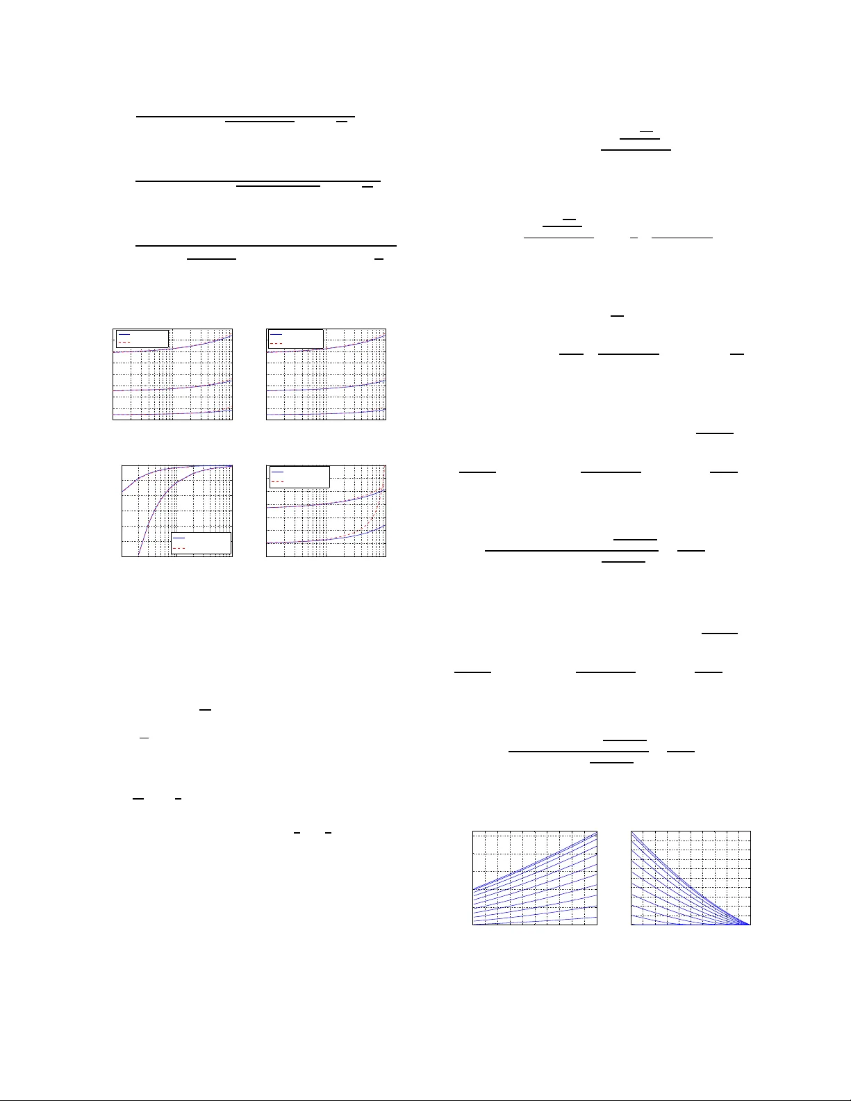
Compr essed Countin g Ping Li Departmen t of Statis tical Science Faculty of Computing and Informatio n Science Cornell University , Ithaca, NY 148 53 pingli@corn ell.edu Abstract Counting is a fundamen tal operation . For exam- ple, coun ting the α th frequen cy moment, F ( α ) = P D i =1 A t [ i ] α , of a streaming signal A t (where t de- notes time), has been an activ e area of research, in theoretical comp uter science, databases, and d ata mining. When α = 1 , the task (i.e., counting th e sum) can be accomp lished using a cou nter . When α 6 = 1 , howe ver , it beco mes non-trivial to d esign a small space (i.e., low memory) counting system. Compr essed Counting (CC) is proposed for effi- ciently compu ting the α th frequency moment of a data stream A t , w here 0 < α ≤ 2 . CC is ap- plicable if the streaming data follow the T urnstile model, with the restriction that at the time t for the ev aluation, A t [ i ] ≥ 0 , ∀ i ∈ [1 , D ] , wh ich includ es the str ict T urnstile model a s a special case. For data streams in practice, this restriction is minor . The under lying technique is skewed stab le random pr ojections , which captures the intuition that, when α = 1 a simple coun ter suffices, an d wh en α = 1 ± ∆ with small ∆ , the sample comp lexity sho uld be lo w (continuo usly as a fu nction of ∆ ). W e sho w the sample complexity (number of projections) k = G 1 ǫ 2 log ` 2 δ ´ , where G = O ( ǫ ) as ∆ → 0 . In other words, f or small ∆ , k = O (1 /ǫ ) instead of O  1 /ǫ 2  . The case ∆ → 0 is pra ctically very importan t. It is now well-understood that one can obtain g ood ap- proxim ations to the entropies of data streams using the α th mom ents with α = 1 ± ∆ an d very small ∆ . F or statistical inference using the metho d of moments , it is sometimes reaso nable use the α th moments with α very close to 1. As another e xam- ple, ∆ might be the “decay rate” or “interest rate, ” which is u sually small. Thus, Comp r essed Count- ing will b e an ideal too l, for estimating the total value in the f uture, tak ing in account th e effect of decaying or interest accruem ent. Finally , our ano ther contribution is an algorithm for ap prox imating the logarithm ic norm, P D i =1 log A t [ i ] , and th e logar ithmic distance, P D i =1 log | A t [ i ] − B t [ i ] | . The lo garithmic norm arises in statistical estima- tions. The logarith mic distance is usefu l in ma- chine learning practice with heavy-tailed data. 1 Intr oduction This pap er focuses o n cou nting , which is amo ng the most fundam ental ope rations in almost e very field o f science and engineer ing. Computing the sum P D i =1 A t [ i ] is the simplest counting ( t denotes time). C ounting th e α th moment P D i =1 A t [ i ] α is more general. When α → 0+ , P D i =1 A i [ i ] α counts the total number of non-zeros in A t . When α = 2 , P D i =1 A t [ i ] α counts the “energy” or “power” of the signal A t . If A t actually out- puts the power of an und erlying signal B t , counting the sum P D i =1 B t is equiv alent to computing P D i =1 A t [ i ] 1 / 2 . Here, A t denotes a time-varying signal, for example, data str eams [8, 5, 10, 2, 4, 17]. In th e liter ature, the α th f requen cy moment of a data stream A t is defined as F ( α ) = D X i =1 | A t [ i ] | α . (1) Counting F ( α ) for massive data streams is practically im- portant, among many challenging issues in data stream com- putations. In fact, the g eneral th eme of “scaling u p f or h igh dimensiona l data and high speed data streams” is among the “ten challenging problem s in data mining research . ” Because th e e lements, A t [ i ] , are time-varying, a n a´ ıve counting mech anism requir es a system of D co unters to com- pute F ( α ) exactly . T his is not al ways realistic when D is large and we only need an app roxima te answer . For exam- ple, D may be 2 64 if A t records the ar riv als of IP addre sses. Or , D can be the total number of checking /savings ac counts. Compressed Counting (CC) is a ne w scheme for approx - imating the α th frequency m oments of data streams (w here 0 < α ≤ 2 ) using low memory . T he underly ing technique is based on what we call skew ed stable random pr ojectio ns . 1.1 The Data Models W e consider the p opular T urnstile d ata stream m odel [17]. The in put stream a t = ( i t , I t ) , i t ∈ [1 , D ] ar riving sequen- tially de scribes the un derlying signal A , mean ing A t [ i t ] = A t − 1 [ i t ] + I t . The increm ent I t can be either positi ve (inser- tion) or negativ e (deletion). Restricting I t ≥ 0 results in the cash r e gister model. Restricting A t [ i ] ≥ 0 at all t (but I t can still be either positive or n egati ve) results in th e strict T u rn- stile mod el, which suffices fo r describing m ost (although not all) natural ph enomen a. For example[ 17 ], in a database, a record can on ly be deleted if it was previously inserted. An- other example is the checking/savings account, which allows deposits/withdrawals b ut generally does not allo w overdraft. Compr essed Counting (CC) is applicable when, at the time t for the ev aluation, A t [ i ] ≥ 0 f or all i . Th is is more flexible than the strict T urnstile model, which req uires A t [ i ] ≥ 0 at all t . In other words, CC is applicable when data streams are ( a) in sertion on ly (i.e ., the cash r e gister model), or (b) always no n-negative (i.e., the strict T urnstile m odel), or (c) non-n egati ve at check po ints. W e b eliev e our model suffices for describin g most natur al data streams in practice. W ith the realistic restriction th at A t [ i ] ≥ 0 at t , the defi- nition of the α th frequen cy momen t becomes F ( α ) = D X i =1 A t [ i ] α ; (2) and the case α = 1 becom es tri vial, because F (1) = D X i =1 A t [ i ] = t X s =1 I s (3) In other words, for F (1) , we need o nly a simple cou nter to accumulate all values of increm ent/decrem ent I t . For α 6 = 1 , howev er , countin g ( 2) is still a non -trivial problem . I ntuitively , there sho uld exist an intelligent cou nt- ing sy stem that perf orms almost like a simple counter when α = 1 ± ∆ with small ∆ . The parameter ∆ may bear a clear physical meaning . For example, ∆ may be the “d ecay rate” or “interest rate, ” which is usually small. The proposed Compr essed C ounting (CC) provides such an intelligent counting systems. Because its underlying tech- nique is based on skewed st able r andom pr ojections , we pro- vide a brief introdu ction to skewed stable distrib utions . 1.2 Skewed Stable Distrib utions A ran dom variable Z f ollows a β -skewed α - stable distribu- tion if the Fourier transform of its density is[21] F Z ( t ) = E exp ` √ − 1 Z t ´ α 6 = 1 , = exp “ − F | t | α “ 1 − √ − 1 β sign ( t ) tan “ π α 2 ””” , where − 1 ≤ β ≤ 1 an d F > 0 is the scale parameter . W e denote Z ∼ S ( α, β , F ) . He re 0 < α ≤ 2 . When α < 0 , the inverse Four ier transfor m is unbounded ; and when α > 2 , th e inverse Fourier transfor m is not a probability density . This is why Compr essed Counting is limited to 0 < α ≤ 2 . Consider two in depend ent variables, Z 1 , Z 2 ∼ S ( α, β , 1) . For any non-negative co nstants C 1 and C 2 , the “ α -stability” follows from properties of F ourier transforms: Z = C 1 Z 1 + C 2 Z 2 ∼ S ( α, β , C α 1 + C α 2 ) . Howe ver , if C 1 and C 2 do not ha ve the same signs, the above “stability” does not hold (unless β = 0 or α = 2 , 0+ ). T o see this, we consider Z = C 1 Z 1 − C 2 Z 2 , with C 1 ≥ 0 and C 2 ≥ 0 . Then, because F − Z 2 ( t ) = F Z 2 ( − t ) , F Z = exp “ −| C 1 t | α “ 1 − √ − 1 β sign ( t ) tan “ π α 2 ””” × exp “ −| C 2 t | α “ 1 + √ − 1 β sign ( t ) tan “ π α 2 ””” , which d oes not represen t a stable law , unless β = 0 or α = 2 , 0+ . This is the fundamen tal r eason why Com pr essed Count- ing need s the restriction that at the time o f ev aluation, ele- ments in the data streams should hav e the same signs. 1.3 Skewed Stable Random Projections Giv en R ∈ R D with each element r i ∼ S ( α, β , 1) i.i.d ., then R T A t = D X i =1 r i A t [ i ] ∼ S α, β , F ( α ) = D X i =1 A t [ i ] α ! , meaning R T A t represents one sample of the stable distribu- tion whose scale parame ter F ( α ) is what we are after . Of c ourse, we need more than one sample to estimate F ( α ) . W e can g enerate a matrix R ∈ R D × k with each entry r ij ∼ S ( α, β , 1) . The resultan t vector X = R T A t ∈ R k contains k i.i.d. samples: x j ∼ S  α, β , F ( α )  , j = 1 to k . Note th at this is a linear pro jection; and recall that the T urnstile mode l is also linear . Thus, skewed stable random pr ojections can be applicable to dynamic data streams. For ev ery in coming a t = ( i t , I t ) , we update x j ← x j + r i t j I t for j = 1 to k . Th is way , at any tim e t , we maintain k i.i.d. stable samples. The remaining task is to recover F ( α ) , which is a statistical estimation problem . 1.4 Counting in Statistical/Learning A pplications The method of moments is ofte n con venient an d popular in statistical parameter estimatio n. Consider, for example, the three-par ameter gen eralized gam ma distribution GG ( θ , γ , η ) , which is h ighly flexible for modelin g positive data, e.g., [15]. If X ∼ GG ( θ , γ , η ) , then the first three moments are E ( X ) = θγ , V ar ( X 2 ) = θ γ 2 , E ( X − E ( X )) 3 = ( η + 1) θγ 3 . T hus, one can estimate θ , γ and η fro m D i.i.d. sam ples x i ∼ GG ( θ, γ , η ) by counting the first thr ee empirical mom ents from the data. Howev er , some moments may be (much) eas- ier to com pute than others if the data x i ’ s are collecte d from data stream s. Instead o f u sing integer mo ments, the param- eters can also be estimated from any th ree fr actional mo- ments, i.e., P D i =1 x α i , for three different values of α . Because D is very large, any co nsistent estimator is likely to provide a good estimate. Thus, it might be reason able to choose α mainly based on the com putationa l cost. See App endix A for comments o n th e situation in which one may also care about the relativ e accuracy caused by different choices of α . The log arithmic no rm P D i =1 log x i arises in statistical es- timation, for e xample, the maximu m likelihood estimator s for the Pareto and gamm a distributions. Since it is closely connected to the moment proble m, Section 4 p rovides an al- gorithm for approximating the lo garithmic nor m, as well as for th e logarithmic distance; the latter can be quite useful in machine learning practice with massive heavy-tailed data (either dynamic or static) in lieu of the usual l 2 distance. Entropy is also an important s ummary statis tic. Recently [20] pr oposed to approxim ate the entropy mo ment P D i =1 x i log x i using the α th mome nts with α = 1 ± ∆ and very small ∆ . 1.5 Comparisons with Previous Studies Pioneered by[1], there have been many studies on approxi- mating the α th frequency mom ent F ( α ) . [1] con sidered in- teger mom ents, α = 0 , 1, 2, as well as α > 2 . Soo n af ter , [5, 9] provid ed improved algorithms for 0 < α ≤ 2 . [18, 3] proved the samp le complexity lo wer bounds for α > 2 . [ 19] proved the optim al lower bounds for all frequ ency moments, except for α = 1 , becau se for no n-negative d ata, F (1) can be computed essentially error-free with a counter [16 , 6, 1]. [11] p rovided algorith ms for α > 2 to (essentially) achieve the lower bounds proved in [ 18, 3]. Note that an algorith m, wh ich “achieves the optimal boun d, ” is not necessarily practical because the constant may be very large. In a sense, the method based on symmetric s table ran- dom pr ojections [10] is on e of the f ew successful algorith ms that are simple and free of large constants. [ 10] described the proced ure fo r approxima ting F (1) in data streams and proved the bound for α = 1 (alth ough n ot explicitly). For α 6 = 1 , [10] provided a c onceptu al algo rithm. [14] pro posed vari- ous estima tors for symmetric stable random pr ojections and provided the constants explicitly for all 0 < α ≤ 2 . None of the pr evious studies, howe ver , c aptures of the intuition that, wh en α = 1 , a simple counter suffices fo r computin g F (1) (essentially) error-free, and when α = 1 ± ∆ with sm all ∆ , the sample comp lexity ( numbe r of projections, k ) should be low and v ary continuously as a function of ∆ . Compressed Co unting ( CC) is proposed f or 0 < α ≤ 2 and it works particularly well when α = 1 ± ∆ with small ∆ . This can be pra ctically very useful. F or examp le, ∆ m ay b e the “decay rate” or the “interest r ate, ” which is usually small; thus CC can count the total value in the fu ture ta king into account the effect of decaying or interest accruement. In pa- rameter estimation s using the method o f momen ts , one may choose the α th moments with α close 1. Also, one can ap- proxim ate the entro py momen t using the α th moments with α = 1 ± ∆ and very small ∆ [20]. Our study has co nnection s to the Joh nson-Lin denstrauss Lemma[1 2 ], which proved k = O  1 /ǫ 2  at α = 2 . An anal- ogous b ound holds f or 0 < α ≤ 2 [1 0, 14]. The depen dency on 1 /ǫ 2 may raise co ncerns if, say , ǫ ≤ 0 . 1 . W e will sho w that CC achie ves k = O (1 /ǫ ) in the neighbo rhood of α = 1 . 1.6 T wo Statistical Estimators Recall that Compr ess ed Counting (CC) boils down to a sta- tistical estimation p roblem . T hat is, given k i.i. d. samp les x j ∼ S  α, β = 1 , F ( α )  , estimate the scale p arameter F ( α ) . Section 2 will explain why we fix β = 1 . Part of this pap er is to p rovide estimators which are con- venient f or theoretical analysis, e.g., tail bound s. W e pro- vide the geometric mean and the ha rmonic mean estimators, whose asymptotic variances are illustrated in Figure 1. 0 0.2 0.4 0.6 0.8 1 1.2 1.4 1.6 1.8 2 0 1 2 3 4 5 α Asymp. variance factor Geometric mean Harmonic mean Symmetric GM Figure 1: Let ˆ F be an estimator of F with asymptotic vari- ance V ar “ ˆ F ” = V F 2 k + O ` 1 k 2 ´ . W e plot the V values for the geometric mea n and the harmonic mean estimators, along with the V values fo r the geometric mean estimator in [14 ] (symmetric GM). When α → 1 , our method achieves an “in- finite improvement” in terms of the asympto tic v ariances. • The geo metric mean estimator , ˆ F ( α ) ,gm ˆ F ( α ) ,gm = Q k j =1 | x j | α/k D gm , ( D gm depends on α and k ) . V ar “ ˆ F ( α ) ,gm ” = F 2 ( α ) k π 2 12 ` α 2 + 2 − 3 κ 2 ( α ) ´ + O „ 1 k 2 « , κ ( α ) = α, if α < 1 , κ ( α ) = 2 − α, if α > 1 . ˆ F ( α ) ,gm is u nbiased. W e pr ove the sample c omplexity explicitly and sho w k = O (1 /ǫ ) suf fices for α aroun d 1. • The harmonic mean estimator, ˆ F ( α ) ,hm,c , for α < 1 ˆ F ( α ) ,hm,c = k cos ( απ 2 ) Γ(1+ α ) P k j =1 | x j | − α „ 1 − 1 k „ 2Γ 2 (1 + α ) Γ(1 + 2 α ) − 1 «« , V ar “ ˆ F ( α ) ,hm,c ” = F 2 ( α ) k „ 2Γ 2 (1 + α ) Γ(1 + 2 α ) − 1 « + O „ 1 k 2 « . It is considerably more accur ate than ˆ F ( α ) ,gm and its sample complexity boun d is also provid ed in an explicit form. Here Γ( . ) is the usual gamma function. 1.7 Paper Organization Section 2 begins with analyzing the moments of ske wed s ta- ble d istributions, from which the geo metric mean and ha r - monic mean estimators ar e derived. Section 2 is then devoted to the detailed analysis of the geometric mean estimator . Section 3 an alyzes the ha rmonic mea n estimator . Section 4 addresses the application of C C in statistical parameter es- timation and an algorithm for app roximatin g the logarithmic norm and distance. The proofs are presented as appendices. 2 The Geometric Mean Estimator W e first p rove a fundam ental r esult ab out th e mom ents of ske wed stable distrib utions. Lemma 1 If Z ∼ S ( α, β , F ( α ) ) , then for any − 1 < λ < α , E “ | Z | λ ” = F λ/α ( α ) cos „ λ α tan − 1 “ β tan “ απ 2 ”” « × “ 1 + β 2 tan 2 “ απ 2 ”” λ 2 α „ 2 π sin “ π 2 λ ” Γ „ 1 − λ α « Γ ( λ ) « , which can be s implified when β = 1 , to be E “ | Z | λ ” = F λ/α ( α ) cos “ κ ( α ) α λπ 2 ” cos λ/α “ κ ( α ) π 2 ” „ 2 π sin “ π 2 λ ” Γ „ 1 − λ α « Γ ( λ ) « , κ ( α ) = α if α < 1 , and κ ( α ) = 2 − α if α > 1 . F or α < 1 , and −∞ < λ < α , E “ | Z | λ ” = E “ Z λ ” = F λ/α ( α ) Γ ` 1 − λ α ´ cos λ/α ` απ 2 ´ Γ (1 − λ ) . Proof: See Append ix B.  Recall that Compr essed Counting boils down to estimat- ing F ( α ) from these k i.i.d. samples x j ∼ S ( α, β , F ( α ) ) . Setting λ = α k in Lemma 1 yields an unbiased estimator: ˆ F ( α ) ,gm,β = Q k j =1 | x j | α/k D gm,β , D gm,β = cos k „ 1 k tan − 1 “ β tan “ απ 2 ”” « × “ 1 + β 2 tan 2 “ απ 2 ”” 1 2 » 2 π sin “ π α 2 k ” Γ „ 1 − 1 k « Γ “ α k ” – k . The following Lemma shows tha t the variance of ˆ F ( α ) ,gm ,β decreases with increasing β ∈ [0 , 1] . Lemma 2 The varianc e of ˆ F ( α ) ,gm ,β V ar “ ˆ F ( α ) ,gm,β ” = F 2 ( α ) V gm,β V gm,β = cos k ` 2 k tan − 1 ` β tan ` απ 2 ´´´ cos 2 k ` 1 k tan − 1 ` β tan ` απ 2 ´´´ × ˆ 2 π sin ` πα k ´ Γ ` 1 − 2 k ´ Γ ` 2 α k ´˜ k ˆ 2 π sin ` πα 2 k ´ Γ ` 1 − 1 k ´ Γ ` α k ´˜ 2 k − 1 , is a decr easing function of β ∈ [0 , 1 ] . Proof: The r esult follows fr o m the fact that cos ` 2 k tan − 1 ` β tan ` απ 2 ´´´ cos 2 ` 1 k tan − 1 ` β tan ` απ 2 ´´´ =2 − sec 2 „ 1 k tan − 1 “ β tan “ απ 2 ”” « , is a deceasing function of β ∈ [0 , 1] .  Therefo re, for attaining th e smallest v ariance, we take β = 1 . For b revity , we simply use ˆ F ( α ) ,gm instead of ˆ F ( α ) ,gm , 1 . In f act, the rest of the paper will always conside r β = 1 o nly . W e r ewrite ˆ F ( α ) ,gm (i.e., ˆ F ( α ) ,gm ,β =1 ) as ˆ F ( α ) ,gm = Q k j =1 | x j | α/k D gm , ( k ≥ 2) , (4) D gm = „ cos k „ κ ( α ) π 2 k « / cos „ κ ( α ) π 2 «« × » 2 π sin “ π α 2 k ” Γ „ 1 − 1 k « Γ “ α k ” – k . Here, κ ( α ) = α , if α < 1 , and κ ( α ) = 2 − α if α > 1 . Lemma 3 concerns the asymptotic moments of ˆ F ( α ) ,gm . Lemma 3 As k → ∞ » cos „ κ ( α ) π 2 k « 2 π Γ “ α k ” Γ „ 1 − 1 k « sin “ π 2 α k ” – k → exp ( − γ e ( α − 1)) , (5) monotonically with incr easing k ( k ≥ 2 ), whe r e γ e = 0 . 5772 4 ... is Euler’ s constant. F or a ny fi xed t , as k → ∞ , E „ “ ˆ F ( α ) ,gm ” t « = F t ( α ) cos k “ κ ( α ) π 2 k t ” ˆ 2 π sin ` πα 2 k t ´ Γ ` 1 − t k ´ Γ ` α k t ´˜ k cos kt “ κ ( α ) π 2 k ” ˆ 2 π sin ` πα 2 k ´ Γ ` 1 − 1 k ´ Γ ` α k ´˜ kt = F t ( α ) exp „ 1 k π 2 ( t 2 − t ) 24 ` α 2 + 2 − 3 κ 2 ( α ) ´ + O „ 1 k 2 «« . V ar “ ˆ F ( α ) ,gm ” = F 2 ( α ) k π 2 12 ` α 2 + 2 − 3 κ 2 ( α ) ´ + O „ 1 k 2 « . Proof: See Appendix C.  In ( 4), the denominator D gm depend s on k for small k . For con venience in analyzing tail bounds, we consid er an asymptotically equiv alent g eometric mean estimator: ˆ F ( α ) ,gm,b = exp ( γ e ( α − 1)) cos „ κ ( α ) π 2 « k Y j =1 | x j | α/k . Lemma 4 provides the tail bo unds for ˆ F ( α ) ,gm ,b and Fig- ure 2 plots the tail bo und constants. One can in fer the tail bound s for ˆ F ( α ) ,gm from the monoton icity result (5). Lemma 4 The right tail bo und: Pr “ ˆ F ( α ) ,gm,b − F ( α ) ≥ ǫF ( α ) ” ≤ exp „ − k ǫ 2 G R,gm « , ǫ > 0 , and the left tail boun d: Pr “ ˆ F ( α ) ,gm,b − F ( α ) ≤ − ǫF ( α ) ” ≤ exp „ − k ǫ 2 G L,gm « , 0 < ǫ < 1 , ǫ 2 G R,gm = C R log(1 + ǫ ) − C R γ e ( α − 1) − log „ cos „ κ ( α ) π C R 2 « 2 π Γ ( αC R ) Γ (1 − C R ) sin „ π αC R 2 «« , ǫ 2 G L,gm = − C L log(1 − ǫ ) + C L γ e ( α − 1) + log α − log „ cos „ κ ( α ) π 2 C L « Γ ( C L ) « + log „ Γ ( αC L ) cos „ π αC L 2 «« . C R and C L ar e solutions to − γ e ( α − 1) + log (1 + ǫ ) + κ ( α ) π 2 tan „ κ ( α ) π 2 C R « − απ / 2 tan ` απ 2 C R ´ − ψ ( αC R ) α + ψ (1 − C R ) = 0 , log(1 − ǫ ) − γ e ( α − 1) − κ ( α ) π 2 tan „ κ ( α ) π 2 C L « + απ 2 tan “ απ 2 C L ” − ψ ( αC L ) α + ψ ( C L ) = 0 . Her e ψ ( z ) = Γ ′ ( z ) Γ( z ) is the “Psi” function . Proof: See Append ix D.  0 0.2 0.4 0.6 0.8 1 0 1 2 3 4 5 6 7 8 9 ε G R,gm α = 0.01 0.99 0.9 0.8 0.7 0.6 0.5 0.4 0.3 0.2 0.1 α = 0.9999 (a) Right bound, α < 1 0 0.2 0.4 0.6 0.8 1 0 2 4 6 8 10 12 14 16 18 ε G R,gm α = 2.0 1.9 1.8 1.7 1.6 1.5 1.4 1.3 1.2 1.1 1.01 1.0001 (b) Right bound, α > 1 0 0.2 0.4 0.6 0.8 1 0 0.5 1 1.5 2 2.5 3 3.5 ε G L,gm α = 0.01 0.1 0.2 0.3 0.4 0.5 0.6 0.7 0.8 0.9 0.99 (c) Left bound, α < 1 0 0.2 0.4 0.6 0.8 1 0 1 2 3 4 5 6 7 8 9 10 ε G L,gm α = 2 1.9 1.8 1.7 1.6 1.5 1.4 1.3 1.2 1.1 1.01 (d) Left bound, α > 1 Figure 2: The tail bound constants of ˆ F ( α ) ,gm ,b in Lemma 4 . It is important to u nderstan d the behavior o f the tail bou nds as α = 1 ± ∆ → 1 . ( α = 1 − ∆ if α < 1 ; and α = 1 + ∆ if α > 1 .) See more comments in Append ix A. Lem ma 5 describes the precise rates of conv ergence. Lemma 5 F or fixed ǫ , as α → 1 (i.e., ∆ → 0 ), G R,gm = ǫ 2 log( 1 + ǫ ) − 2 p ∆ log (1 + ǫ ) + o “ √ ∆ ” , If α > 1 , then G L,gm = ǫ 2 − log ( 1 − ǫ ) − 2 p − 2∆ log(1 − ǫ ) + o “ √ ∆ ” , If α < 1 , then G L,gm = ǫ 2 ∆ “ exp “ − l og (1 − ǫ ) ∆ − 1 − γ e ”” + o ` ∆ exp ` 1 ∆ ´´ . Proof: See Append ix E .  10 −4 10 −3 10 −2 0 0.5 1 1.5 2 ∆ ( α <1) G R,gm ε = 1.0 ε = 0.1 ε = 0.5 Exact Approximate (a) Right bound, α < 1 10 −4 10 −3 10 −2 0 0.5 1 1.5 2 ∆ ( α >1) G R,gm ε = 1.0 ε = 0.5 ε = 0.1 Exact Approximate (b) Right bound, α > 1 10 −3 10 −2 10 −1 10 −150 10 −125 10 −100 10 −75 10 −50 10 −25 10 0 ∆ ( α <1) G L,gm ε = 0.5 ε = 0.1 Exact Approximate (c) Left bound, α < 1 10 −4 10 −3 10 −2 0 0.1 0.2 0.3 0.4 0.5 0.6 0.7 ∆ ( α >1) G L,gm ε = 0.5 ε = 0.1 Exact Approximate (d) Left bound, α > 1 Figure 3: The tail bound constants proved in Lemma 4 and the approx imations in Lemma 5, for small ∆ . Figure 3 plo ts the constants f or small values of ∆ , a long with the appr oximation s sugg ested in Lemma 5. Since we usually consider ǫ should not be too large, we can write, as α → 1 , G R,gm = O ( ǫ ) and G L,g m = O ( ǫ ) if α > 1 ; both at the rate O “ √ ∆ ” . Howe ver , if α < 1 , G L,gm = O ` ǫ exp ` − ǫ ∆ ´´ , which is extremely fast. The sample complexity bo und is then straightforward. Lemma 6 Using the geometric mean estimator , it suffices t o let k = G 1 ǫ 2 log  2 δ  so tha t the err or will be within a 1 ± ǫ factor with pr obability 1 − δ , wher e G = max( G R,gm , G L,g m ) . In the neighbo rhood of α = 1 , k = O  1 ǫ log 2 δ  only . 3 The Harmonic Mean Estimator For α < 1 , th e harmonic mean estimator can considerably improve ˆ F ( α ) ,gm . Unlike the harmo nic mean e stimator in [14], which is useful only for small α a nd has no exponential tail boun ds except for α = 0+ , the h armonic mean estimator in this study has very nice tail properties for all 0 < α < 1 . The harmonic mean estimator takes advantage of the fact that if Z ∼ S ( α < 1 , β = 1 , F ( α ) ) , then E  | Z | λ  = E  Z λ  exists for all −∞ < λ < α . Lemma 7 Assume k i.i.d. samples x j ∼ S ( α < 1 , β = 1 , F ( α ) ) , define the harmonic mean estimator ˆ F ( α ) ,hm , ˆ F ( α ) ,hm = k cos ( απ 2 ) Γ(1+ α ) P k j =1 | x j | − α , and the bias-corr ected harmo nic mean estimator ˆ F ( α ) ,hm,c , ˆ F ( α ) ,hm,c = k cos ( απ 2 ) Γ(1+ α ) P k j =1 | x j | − α „ 1 − 1 k „ 2Γ 2 (1 + α ) Γ(1 + 2 α ) − 1 «« . The bias and variance of ˆ F ( α ) ,hm,c ar e E “ ˆ F ( α ) ,hm,c ” = F ( α ) + O „ 1 k 2 « , V ar “ ˆ F ( α ) ,hm,c ” = F 2 ( α ) k „ 2Γ 2 (1 + α ) Γ(1 + 2 α ) − 1 « + O „ 1 k 2 « . The right tail bound of ˆ F ( α ) ,hm is, for ǫ > 0 , Pr “ ˆ F ( α ) ,hm − F ( α ) ≥ ǫF ( α ) ” ≤ exp „ − k „ ǫ 2 G R,hm «« , ǫ 2 G R,hm = − log ∞ X m =0 Γ m (1 + α ) Γ(1 + mα ) ( − t ∗ 1 ) m ! − t ∗ 1 1 + ǫ , wher e t ∗ 1 is the solution to P ∞ m =1 ( − 1) m m ( t ∗ 1 ) m − 1 Γ m (1+ α ) Γ(1+ mα ) P ∞ m =0 ( − 1) m ( t ∗ 1 ) m Γ m (1+ α ) Γ(1+ mα ) + 1 1 + ǫ = 0 . The left tail bound of ˆ F ( α ) ,hm is, for 0 < ǫ < 1 , Pr “ ˆ F ( α ) ,hm − F ( α ) ≤ − ǫF ( α ) ” ≤ exp „ − k „ ǫ 2 G L,hm «« , ǫ 2 G L,hm = − log ∞ X m =0 Γ m (1 + α ) Γ(1 + mα ) ( t ∗ 2 ) m ! + t ∗ 2 1 − ǫ wher e t ∗ 2 is the solution to − P ∞ m =1 m ( t ∗ 2 ) m − 1 Γ m (1+ α ) Γ(1+ mα ) P ∞ m =0 ( t ∗ 2 ) m Γ m (1+ α ) Γ(1+ mα ) + 1 1 − ǫ = 0 Proof: See Append ix F.  . 0 0.2 0.4 0.6 0.8 1 0 1 2 3 4 5 ε G R,hm α = 0.01 0.2 0.4 0.3 0.5 0.6 0.1 0.7 0.8 0.9 0.99 (a) Right tail bound constant 0 0.2 0.4 0.6 0.8 1 0 0.4 0.8 1.2 1.6 2 ε G L,hm α = 0.01 0.1 0.2 0.3 0.4 0.5 0.6 0.8 0.9 0.99 0.7 (b) Left tail bound constant Figure 4: The tail bound con stants of ˆ F ( α ) ,hm in Lemma 7, which are considerab ly s maller , compared to Figure 2(a)(c). 4 The Logarithmic Norm and Distance The logarithmic n orm and distance can be impo rtant in prac- tice. Consider estimating the parameter s fro m D i.i.d. sam- ples x i ∼ Gamma ( θ , γ ) . Th e density functio n is f X ( x ) = x θ − 1 exp( − x/γ ) γ θ Γ( θ ) , and the likelihood equation is ( θ − 1) D X i =1 log x i − D X i =1 x i /γ − Dθ log( γ ) − D log Γ( θ ) . If in stead, x i ∼ P ar eto ( θ ) , i = 1 to D , th en the d ensity is f X ( x ) = θ x θ +1 , x ≥ 1 , and the likelihood equation is D log θ − ( θ + 1) D X i =1 log x i . Therefo re, the lo garithmic norm oc curs at least in the content of m aximum likelihood estimations o f comm on dis- tributions. Now , consider the d ata x i ’ s are actually the el- ements of data streams A t [ i ] ’ s . Estimating P D i =1 log A t [ i ] becomes an interesting and practically meaningfu l pro blem. Our solution is based on the fact that, as α → 0 + , D α log 1 D D X i =1 A t [ i ] α ! → D X i =1 log A t [ i ] , which can be shown by L ’H ´ opital’ s rule. More precisely , ˛ ˛ ˛ ˛ ˛ D α log 1 D D X i =1 A t [ i ] α ! − D X i =1 log A t [ i ] ˛ ˛ ˛ ˛ ˛ = O 0 @ α D D X i =1 log A t [ i ] ! 2 1 A + O α D X i =1 log 2 A t [ i ] ! , which can be shown by T aylor expansions. Therefo re, we obtain one solution to ap proxim ating the logarithm ic norm using very small α . Of cour se, we have assumed that A t [ i ] > 0 strictly . In fact, this also su ggests an ap proach for appr oximating the lo garithmic d istance b e- tween two streams P D i =1 log | A t [ i ] − B t [ i ] | , provided we use symmetric stable random pr ojec tions . The logarithmic distance can be useful in machine learn- ing practice with massi ve h eavy-tailed data (eithe r static or dynamic) such as image and text data. For those d ata, the usual l 2 distance would n ot be useful withou t “term-weigh ting” the data; and tak ing logar ithm is one simp le weightin g scheme. Thus, our method provides a direct way t o compute pairwise distances, taking into account data weighting automatically . One may be also interested in the tail bo unds, which, howe ver , c an not b e expressed in terms of the logarithm ic norm (or distance). Ne vertheless, we can obtain , e.g., Pr „» D α log „ 1 D ˆ F ( α ) ,hm «– ≥ (1 + ǫ ) » D α log „ 1 D F ( α ) «–« ≤ exp − k `` F ( α ) /D ´ ǫ − 1 ´ 2 G R,hm ! , ǫ > 0 , Pr „» D α log „ 1 D ˆ F ( α ) ,hm «– ≤ (1 − ǫ ) » D α log „ 1 D F ( α ) «–« ≤ exp − k ` 1 − ` D/F ( α ) ´ ǫ ´ 2 G L,hm ! , 0 < ǫ < 1 If ˆ F ( α ) ,gm is used, w e just replace the corre sponding co n- stants in the ab ove expression s. If w e are in terested in the logarithm ic distance, we simply apply symmetric stable r an- dom pr ojections and use an ap prop riate estimator of the d is- tance; the correspon ding t ail boun ds will have same format. 5 Conclusion Counting is a fundamental o peration . In data strea ms A t [ i ] , i ∈ [1 , D ] , countin g the α th fr equency moments F ( α ) = P D i =1 A t [ i ] α has been extensively studied . Our prop osed Compr essed Countin g ( CC) takes adv antage of th e fact that most data streams en counter ed in practice are no n-negative, although they ar e subject to deletion and insertion. In fact, CC only requ ires th at at the time t f or the ev aluation, A t [ i ] ≥ 0 ; at other times, the d ata strea ms can actually go below zero. Compr essed Counting successfully captures the intuition that, wh en α = 1 , a simp le counter suffices, a nd when α = 1 ± ∆ with small ∆ , an intelligent counting system should require low space (continuou sly as a function o f ∆ ). The case with small ∆ c an be practically important. For exam- ple, ∆ may be the “d ecay rate” o r “interest r ate, ” which is usually small. CC ca n also be very useful for statistical pa- rameter estimation based o n the method of moments . Also, one can app roxima te the entr opy moment using the α th mo- ments with α = 1 ± ∆ and very small ∆ . Compared with p revious studies, e.g ., [10, 14], Com- pr essed Countin g achieves, in a sense, an “infinite improve- ment” in term s o f th e asymp totic variances wh en ∆ → 0 . T wo estimators based on the geometr ic mean and the har- monic mea n are pr ovided in this stu dy , includ ing th eir vari- ances, tail boun ds, and samp le complexity bounds. W e analy ze ou r sample complexity boun d k = G 1 ǫ 2 log 2 δ at the neigh borho od of α = 1 and show G = O ( ǫ ) at small ∆ . This implies that our b ound at small ∆ is actu- ally k = O (1 /ǫ ) in stead of O  1 /ǫ 2  , which is req uired in the Johnson-L indenstrau ss Lemma and its v arious analogs. Finally , we propo se a scheme for appr oximating the log- arithmic norm and the logar ithmic distance , useful in statis- tical parameter estimation and machine learning practice. W e expect that new algorithm s will soon be developed to take adv antage of Compr es sed Counting . For examp le, via private communications, we have learned that a gro up is vigoro usly developing algo rithms using projections with α = 1 ± ∆ very close to 1, whe re ∆ is their important parameter . A An Example of Method of Moments W e p rovide a (somewhat con triv ed) example of th e method of moments . Sup pose the o bserved data x i ’ s are from data streams and suppose the data f ollows a gamma distribution x i ∼ Gamma ( θ , 1) , i.i.d . Here, we only con sider o ne pa- rameter θ so that we can analyze the variance easily . Suppose we estimate θ u sing the α th m oment. Because E ( x α i ) = Γ( α + θ ) / Γ( θ ) , we can solve for ˆ θ from Γ( α + ˆ θ ) Γ( ˆ θ ) = 1 D D X i =1 x α k , = ⇒ V ar Γ( α + ˆ θ ) Γ( ˆ θ ) ! = 1 D Γ(2 α + θ ) Γ( θ ) − Γ 2 ( α + θ ) Γ 2 ( θ ) ! By the ”delta meth od” ( i.e., V ar ( h ( x )) ≈ V ar ( x )( h ′ ( E ( x ))) 2 ) and using the implicit deriv ativ e of ˆ θ , we obtain V ar “ ˆ θ ” ≈ 1 D „ Γ(2 α + θ )Γ( θ ) Γ 2 ( α + θ ) − 1 « 1 ( ψ ( α + θ ) − ψ ( θ )) 2 . One ca n verify V ar ( ˆ θ ) increases monoto nically with in- creasing α ∈ [0 , ∞ ) . Because x i ’ s are fr om data streams, we apply Compressed Counting for the α th mo ment. Sup- pose we consider the dif ference in the estimation accuracy at different α is not important (because D is large). Then we simply let α = 1 . In case we need to estimate two parame- ters, we might choose α = 1 and anoth er α close to 1. Now supp ose we actually car e abou t both the estimation accuracy (which fa vors smaller α ) and the computational ef- ficiency (wh ich fav ors α = 1 ), we the n n eed to ba lance th is trade-off by cho osing α . T o do so, we need to know the pre- cise behavior of Compr ess ed Cou nting in th e neig hbor hood of α = 1 , as well as the pr ecise behavior of ˆ θ , i. e., its tail bound s (not just v ariance). Thu s, our analysis on the conv er- gence rates in Lemma 5 will be very useful. B Proof of Lemma 1 Assume Z ∼ S ( α, β , F ( α ) ) . T o prove E  | Z | λ  for − 1 < λ < α , [21, Theorem 2.6.3] provided on ly a partial answer: Z ∞ 0 z λ f Z ( z ; α, β B , F ( α ) ) dz = F λ/α ( α ) sin( πρλ ) sin( π λ ) Γ ` 1 − λ α ´ Γ (1 − λ ) cos − λ/α ( π β B κ ( α ) / 2) where we denote κ ( α ) = α if α < 1 , and κ ( α ) = 2 − α if α > 1 , and according to the parame trization u sed in [21, I.19, I.28]: β B = 2 π κ ( α ) tan − 1 „ β tan „ π α 2 «« , ρ = 1 − β B κ ( a ) /α 2 . Note that cos − λ/α ( π β B κ ( α ) / 2) = “ 1 + tan 2 ( π β B κ ( α ) / 2) ” λ 2 α = „ 1 + tan 2 „ tan − 1 „ β tan „ π α 2 «««« λ 2 α = „ 1 + β 2 tan 2 „ π α 2 «« λ 2 α . Therefo re, for − 1 < λ < α , Z ∞ 0 z λ f Z ( z ; α, β B , F ( α ) ) dz = F λ/α ( α ) sin( π ρλ ) sin( π λ ) Γ ` 1 − λ α ´ Γ (1 − λ ) „ 1 + β 2 tan 2 „ π α 2 «« λ 2 α . T o compu te E  | Z | λ  , we take advantage of a useful pro p- erty of the stable density function [21 , page 65]: f Z ( − z ; α, β B , F ( α ) ) = f Z ( z ; α, − β B , F ( α ) ) . E “ | Z | λ ” = Z 0 −∞ ( − z ) λ f Z ( z ; α, β B , F ( α ) ) dz + Z ∞ 0 z λ f Z ( z ; α, β B , F ( α ) ) dz = Z ∞ 0 z λ f Z ( z ; α, − β B , F ( α ) ) dz + Z ∞ 0 z λ f Z ( z ; α, β B , F ( α ) ) dz = F λ/α ( α ) sin( π λ ) Γ ` 1 − λ α ´ Γ (1 − λ ) „ 1 + β 2 tan 2 „ π α 2 «« λ 2 α × „ sin „ π λ 1 − β B κ ( α ) /α 2 « + sin „ π λ 1 + β B κ ( α ) /α 2 «« = F λ/α ( α ) sin( π λ ) Γ ` 1 − λ α ´ Γ (1 − λ ) „ 1 + β 2 tan 2 „ π α 2 «« λ 2 α × „ 2 sin „ π λ 2 « cos „ π λ 2 β B κ ( α ) /α «« = F λ/α ( α ) cos( π λ/ 2) Γ ` 1 − λ α ´ Γ (1 − λ ) „ 1 + β 2 tan 2 „ π α 2 «« λ 2 α × cos „ λ α tan − 1 „ β tan „ π α 2 ««« = F λ/α ( α ) „ 1 + β 2 tan 2 „ π α 2 «« λ 2 α cos „ λ α tan − 1 „ β tan „ π α 2 ««« × „ 2 π sin „ π 2 λ « Γ „ 1 − λ α « Γ ( λ ) « , which can be simplified when β = 1 , to be E “ | Z | λ ” = F λ/α ( α ) cos “ κ ( α ) α λπ 2 ” cos λ/α “ κ ( α ) π 2 ” „ 2 π sin „ π 2 λ « Γ „ 1 − λ α « Γ ( λ ) « . The final task is to show that when α < 1 an d β = 1 , E  | Z | λ  exists for all −∞ < λ < α , not ju st − 1 < λ < α . This is an extremely useful property . Note that when α < 1 a nd β = 1 , Z is always non- negativ e. As shown in th e proof of [21, Theorem 2.6.3], E “ | Z | λ ” = F λ/α ( α ) cos − λ/α „ π α 2 « 1 π Im Z ∞ 0 z λ Z ∞ 0 exp − z u exp( √ − 1 π / 2) − u α exp( − √ − 1 π α/ 2) + √ − 1 π 2 ! dudz = F λ/α ( α ) cos − λ/α „ π α 2 « 1 π × Im Z ∞ 0 Z ∞ 0 z λ exp ` − z u √ − 1 − u α exp( − √ − 1 π α/ 2) ´ √ − 1 dudz . The on ly thing we need to chec k is that in the proo f of [ 21, Theorem 2.6.3] , the co ndition for Fubini’ s theorem (to ex- change ord er of in tegration) still ho lds when − ∞ < α < 1 , β = 1 , and λ < − 1 . W e ca n show Z ∞ 0 Z ∞ 0 ˛ ˛ ˛ z λ exp ` − z u √ − 1 − u α exp( − √ − 1 π α/ 2) ´ √ − 1 ˛ ˛ ˛ dudz = Z ∞ 0 Z ∞ 0 z λ ˛ ˛ exp ` − u α cos( π α/ 2) + √ − 1 u α sin( π α/ 2) ´ ˛ ˛ dudz = Z ∞ 0 Z ∞ 0 z λ exp ` − u α cos( π α/ 2) ´ dudz < ∞ , provided λ < − 1 ( λ 6 = − 1 , − 2 , − 3 , .... ) and cos( π α/ 2) > 0 , i.e., α < 1 . Note that | exp( √ − 1 x ) | = 1 always and Euler’ s formu la: exp( √ − 1 x ) = c o s( x ) + √ − 1 s in( x ) is frequen tly used to simplify the algeb ra. Once we show that Fubini’ s conditio n is satisfied, we can exchange the or der o f integration and the rest follows from the pro of of [21, Theo rem 2.6.3 ]. Because of continu ity , the “singularity points” λ = − 1 , − 2 , − 3 , ... do not matter . C Proof of L emma 3 W e first show that, for any fixed t , as k → ∞ , E ““ ˆ F ( α ) ,gm ” t ” = F t ( α ) cos k “ κ ( α ) π 2 k t ” ˆ 2 π sin ` πα 2 k t ´ Γ ` 1 − t k ´ Γ ` α k t ´˜ k cos kt “ κ ( α ) π 2 k ” ˆ 2 π sin ` πα 2 k ´ Γ ` 1 − 1 k ´ Γ ` α k ´˜ kt = F t ( α ) exp 1 k π 2 ( t 2 − t ) 24 “ α 2 + 2 − 3 κ 2 ( α ) ” + O „ 1 k 2 « ! . In [14], it was proved that, as k → ∞ , ˆ 2 π sin ` πα 2 k t ´ Γ ` 1 − t k ´ Γ ` α k t ´˜ k ˆ 2 π sin ` πα 2 k ´ Γ ` 1 − 1 k ´ Γ ` α k ´˜ kt =1 + 1 k π 2 ( t 2 − t ) 24 “ α 2 + 2 ” + O „ 1 k 2 « = ex p 1 k π 2 ( t 2 − t ) 24 “ α 2 + 2 ” + O „ 1 k 2 « ! . Using the infin ite p roduct representation o f cosine[7, 1.43.3] cos( z ) = ∞ Y s =0 1 − 4 z 2 (2 s + 1) 2 π 2 ! , we can rewrite cos k “ κ ( α ) π 2 k t ” cos kt “ κ ( α ) π 2 k ” = ∞ Y s =0 1 − κ 2 ( α ) t 2 (2 s + 1) 2 k 2 ! k 1 − κ 2 ( α ) (2 s + 1) 2 k 2 ! − kt = ∞ Y s =0 1 − κ 2 ( α ) t 2 (2 s + 1) 2 k 2 ! 1 + t κ 2 ( α ) (2 s + 1) 2 k 2 + O „ 1 k 3 « !! k = ∞ Y s =0 1 − κ 2 ( α )( t 2 − t ) (2 s + 1) 2 k 2 + O „ 1 k 3 « ! k = ∞ Y s =0 1 − κ 2 ( α )( t 2 − t ) (2 s + 1) 2 k + O „ 1 k 2 « ! = ex p ∞ X s =0 log 1 − κ 2 ( α )( t 2 − t ) (2 s + 1) 2 k + O „ 1 k 2 « !! = ex p − κ 2 ( α ) k ( t 2 − t ) ∞ X s =0 1 (2 s + 1) 2 + O „ 1 k 2 « ! = ex p − κ 2 ( α ) k ( t 2 − t ) π 2 8 + O „ 1 k 2 « ! , which, combined with the result in [14], yields the desired expression. The next task i s to show » cos „ κ ( α ) π 2 k « 2 π Γ „ α k « Γ „ 1 − 1 k « sin „ π 2 α k «– k → exp ( − γ e ( α − 1)) , monoto nically as k → ∞ , where γ e = 0 . 5772156 65 ... , is Euler’ s con stant. In [1 4], it was proved that, as k → ∞ , » 2 π Γ „ α k « Γ „ 1 − 1 k « sin „ π 2 α k «– k → exp ( − γ e ( α − 1)) , monoto nically . In this study , we need to conside r instead » cos „ κ ( α ) π 2 k « 2 π Γ „ α k « Γ „ 1 − 1 k « sin „ π 2 α k «– k = " 2 cos „ κ ( α ) π 2 k « Γ ` α k ´ sin ` πα 2 k ´ Γ ` 1 k ´ sin ` π k ´ # k (6) (Note E uler’ s reflection formula Γ( z )Γ(1 − z ) = π sin( π z ) .) The additiona l term h cos “ κ ( α ) π 2 k ”i k = 1 − O ` 1 k ´ . Therefore, » cos „ κ ( α ) π 2 k « 2 π Γ „ α k « Γ „ 1 − 1 k « sin „ π 2 α k «– k → exp ( − γ e ( α − 1)) . T o sho w the monotonicity , h owe ver , we have to use som e different tech niques from [14 ]. The r eason is becau se the ad- ditional term h cos  κ ( α ) π 2 k i k increases (instead o f decrea s- ing) mono tonically with increasin g k . First, w e consider α > 1 , i.e., κ ( α ) = 2 − α < 1 . For simplicity , we take lo garithm of (6) an d rep lace 1 /k by t , where 0 ≤ t ≤ 1 / 2 (r ecall k ≥ 2 ). I t suf fices to show tha t g ( t ) incre ases with increasing t ∈ [0 , 1 / 2] , where g ( t ) = 1 t W ( t ) , W ( t ) = log „ cos „ κ ( α ) π 2 t «« + log (Γ ( αt )) + l og „ sin „ π α 2 t «« − log (Γ ( t )) − log (sin ( π t )) + log (2) . Because g ′ ( t ) = 1 t W ′ ( t ) − 1 t 2 W ( t ) , to show g ′ ( t ) ≥ 0 in t ∈ [0 , 1 / 2] , it suffices to show tW ′ ( t ) − W ( t ) ≥ 0 . One can check that tW ′ ( t ) → 0 an d W ( t ) → 0 , as t → 0+ . W ′ ( t ) = − tan „ κ ( α ) π 2 t « „ κπ 2 « + ψ ( αt ) α + 1 tan ` πα 2 t ´ „ απ 2 « − ψ ( t ) − 1 tan( π t ) π . Here ψ ( x ) = ∂ log(Γ( x )) ∂ x is the “Psi” fu nction. Therefo re, to show tW ′ ( t ) − W ( t ) ≥ 0 , it suffices to show that tW ′ ( t ) − W ( t ) is an increasing function of t ∈ [0 , 1 / 2] , i.e., ` tW ′ ( t ) − W ( t ) ´ ′ = W ′′ ( t ) ≥ 0 , i.e., W ′′ ( t ) = − sec 2 „ κ ( α ) π 2 t « „ κ ( α ) π 2 « 2 + ψ ′ ( αt ) α 2 − csc 2 „ π α 2 t « „ π α 2 « 2 − ψ ′ ( t ) + csc 2 ( π t ) π 2 ≥ 0 . Using series r epresentation of ψ ( x ) [ 7, 8.363.8 ], we show ψ ′ ( αt ) α 2 − ψ ′ ( t ) = ∞ X s =0 α 2 ( αt + s ) 2 − ∞ X s =0 1 ( t + s ) 2 = ∞ X s =0 „ 1 ( t + s/α ) 2 − 1 ( t + s ) 2 « ≥ 0 , because we consider α > 1 . Th us, it suf fices to show that Q ( t ; α ) = − sec 2 „ κ ( α ) π 2 t « „ κ ( α ) π 2 « 2 − csc 2 „ π α 2 t « „ π α 2 « 2 + csc 2 ( π t ) π 2 ≥ 0 . T o show Q ( t ; α ) ≥ 0 , we can treat Q ( t ; α ) as a fu nction o f α (for fixed t ). Becau se b oth 1 sin( x ) and 1 cos( x ) are co n vex function s of x ∈ [0 , π / 2] , we k now Q ( t ; α ) is a concave function of α (for fixed t ). It is easy to c heck that lim α → 1+ Q ( t ; α ) = 0 , lim α → 2 − Q ( t ; α ) = 0 . Because Q ( t ; α ) is concave in α ∈ [1 , 2 ] , we must have Q ( t ; α ) ≥ 0 ; and co nsequently , W ′′ ( t ) ≥ 0 and g ′ ( t ) ≥ 0 . Therefo re, we have proved that (6) decre ases monoto nically with increasing k , when 1 < α ≤ 2 . For α < 1 (i.e., κ ( α ) = α < 1 ), we prove the mono- tonicity by a different tech nique. First, using infinite- produ ct representatio ns [7, 8.3 22,1. 431.1 ], Γ( z ) = exp ( − γ e z ) z ∞ Y s =1 „ 1 + z s « − 1 exp „ z s « , sin( z ) = z ∞ Y s =1 1 − z 2 s 2 π 2 ! , we can rewrite (6) as " 2 cos „ κ ( α ) π 2 k « Γ ` α k ´ sin ` πα 2 k ´ Γ ` 1 k ´ sin ` π k ´ # k = e x p ( − γ e ( α − 1)) × ∞ Y s =1 exp „ α − 1 sk « „ 1 + α ks « − 1 „ 1 + 1 ks « 1 − α 2 k 2 s 2 ! „ 1 − 1 s 2 k 2 « − 1 ! k . T o show its monoton icity , it suf fices to sho w for any s ≥ 1 „ 1 + α ks « − 1 „ 1 + 1 ks « 1 − α 2 k 2 s 2 ! „ 1 − 1 s 2 k 2 « − 1 ! k decreases mo noton ically , wh ich is equi valent to sho w the monoto nicity of g ( t ) with incr easing t , for t ≥ 2 , where g ( t ) = t log „ 1 + α t « − 1 „ 1 + 1 t « 1 − α 2 t 2 ! „ 1 − 1 t 2 « − 1 ! = t log „ t − α t − 1 « . It is stra ightforward to show that t lo g  t − α t − 1  is mono toni- cally decreasing with increasing t ( t ≥ 2 ), for α < 1 . T o th is end, we have proved that for 0 < α ≤ 2 ( α 6 = 1 ), » cos „ κ ( α ) π 2 k « 2 π Γ „ α k « Γ „ 1 − 1 k « sin „ π 2 α k «– k → exp ( − γ e ( α − 1)) , monoto nically with incr easing k ( k ≥ 2 ). D Proof of L emma 4 W e first fin d the constant G R,gm in the right tail bound Pr “ ˆ F ( α ) ,gm,b − F ( α ) ≥ ǫF ( α ) ” ≤ e xp − k ǫ 2 G R,gm ! , ǫ > 0 . For 0 < t < k , the Markov moment bound yields Pr “ ˆ F ( α ) ,gm,b − F ( α ) ≥ ǫF ( α ) ” ≤ E “ ˆ F ( α ) ,gm ” t (1 + ǫ ) t F t ( α ) = h cos “ κ ( α ) π 2 k t ” 2 π Γ ` αt k ´ Γ ` 1 − t k ´ sin ` παt 2 k ´ i k (1 + ǫ ) t exp ( − tγ e ( α − 1)) . W e need to find the t that minimizes the upper bou nd. For conv enience, we consider its log arithm, i.e., g ( t ) = tγ e ( α − 1) − t log(1 + ǫ )+ k log „ cos „ κ ( α ) π 2 k t « 2 π Γ „ αt k « Γ „ 1 − t k « sin „ π αt 2 k «« , whose first and second deriv ati ves (with respect to t ) are g ′ ( t ) = γ e ( α − 1) − log(1 + ǫ ) − κ ( α ) π 2 tan „ κ ( α ) π 2 k t « + απ/ 2 tan ` απt 2 k ´ + ψ „ αt k « α − ψ „ 1 − t k « , tg ′′ ( t ) = − „ κ ( α ) π 2 « 2 sec 2 „ κ ( α ) π 2 k t « − „ απ 2 « 2 csc 2 „ απt 2 k « + α 2 ψ ′ „ αt k « + ψ ′ „ 1 − t k « . W e need to show that g ( t ) is a c onv ex func tion. By the following e xpansions: [7, 1 .422. 2, 1.42 2.4, 8.363.8] sec 2 „ π x 2 « = 4 π 2 ∞ X j =1 „ 1 (2 j − 1 − x ) 2 + 1 (2 j − 1 + x ) 2 « , csc 2 ( π x ) = 1 π 2 x 2 + 2 π 2 ∞ X j =1 x 2 + j 2 ( x 2 − j 2 ) 2 , ψ ′ ( x ) = ∞ X j =0 1 ( x + j ) 2 , we can rewrite kg ′′ ( t ) = − κ 2 ∞ X j =1 „ 1 (2 j − 1 − κt/k ) 2 + 1 (2 j − 1 + κt/k ) 2 « − k 2 t 2 − α 2 2 ∞ X j =1 ( αt/ 2 k ) 2 + j 2 (( αt/ 2 k ) 2 − j 2 ) 2 + α 2 ∞ X j =0 1 ( αt/k + j ) 2 + ∞ X j =0 1 (1 − t/k + j ) 2 = − κ 2 ∞ X j =1 „ 1 (2 j − 1 − κt/k ) 2 + 1 (2 j − 1 + κt/k ) 2 « − α 2 ∞ X j =1 „ 1 ( αt/k − 2 j ) 2 + 1 ( αt/k + 2 j ) 2 « + α 2 ∞ X j =1 1 ( αt/k + j ) 2 + ∞ X j =1 1 ( j − t/k ) 2 . If α < 1 , i.e., κ ( α ) = α , the n kg ′′ ( t ) = − α 2 ∞ X j =1 „ 1 ( αt/k − j ) 2 + 1 ( αt/k + j ) 2 « + α 2 ∞ X j =1 1 ( αt/k + j ) 2 + ∞ X j =1 1 ( j − t/k ) 2 = − α 2 ∞ X j =1 1 ( j − αt/k ) 2 + ∞ X j =1 1 ( j − t/k ) 2 ≥ 0 , because α < 1 and 0 < t < k . If α > 1 , i.e., κ ( α ) = 2 − α < 1 , then kg ′′ ( t ) = − κ 2 ∞ X j =1 „ 1 (2 j − 1 − κt/k ) 2 + 1 (2 j − 1 + κt/k ) 2 « − α 2 ∞ X j =1 „ 1 ( αt/k − 2 j ) 2 + 1 ( αt/k + 2 j ) 2 « + α 2 ∞ X j =1 1 ( αt/k + 2 j ) 2 + α 2 ∞ X j =1 1 ( αt/k + 2 j − 1) 2 + ∞ X j =1 1 (2 j − t/k ) 2 + ∞ X j =1 1 (2 j − 1 − t/k ) 2 ≥ − κ 2 ∞ X j =1 1 (2 j − 1 + κt/k ) 2 − α 2 ∞ X j =1 1 (2 j − αt/k ) 2 + α 2 ∞ X j =1 1 ( αt/k + 2 j − 1) 2 + ∞ X j =1 1 (2 j − t/k ) 2 = 0 @ − ∞ X j =1 1 ((2 j − 1) /κ + t/k ) 2 + ∞ X j =1 1 ((2 j − 1) /α + t/k ) 2 1 A + 0 @ − ∞ X j =1 1 (2 j /α − t/k ) 2 + ∞ X j =1 1 (2 j − t/k ) 2 1 A ≥ 0 , ( because α > κ ) . Since we have proved that g ′′ ( t ) , i.e., g ( t ) is a c onv ex function , one can find the op timal t by solving g ′ ( t ) = 0 : γ e ( α − 1) − log(1 + ǫ ) − κ ( α ) π 2 tan „ κ ( α ) π 2 k t « + απ/ 2 tan ` απt 2 k ´ + + ψ „ αt k « α − ψ „ 1 − t k « = 0 , W e let the solution be t = C R k , where C R is the solution to γ e ( α − 1) − l og(1 + ǫ ) − κ ( α ) π 2 tan „ κ ( α ) π 2 C R « + απ/ 2 tan ` απ 2 C R ´ + ψ ( αC R ) α − ψ (1 − C R ) = 0 . Alternatively , we can seek a “sub -optimal” (but asymp- totically optimal) solu tion using the asym ptotic expression for E “ ˆ F ( α ) ,gm ” t in Lemma 3, i.e., the t that minimizes (1 + ǫ ) − t exp 1 k π 2 24 “ t 2 − t ” “ 2 + α 2 − 3 κ 2 ( α ) ” ! , whose minimum is attained at t = k log(1 + ǫ ) (2 + α 2 − 3 κ 2 ( α )) π 2 / 12 + 1 2 . This appr oximation can be useful (e.g., ) for servin g the ini- tial guess for C R in a numerica l procedure. Assume we know C R (e.g., b y a numerical procedur e), we can then express the right tail bound as Pr “ ˆ F ( α ) ,gm,b − F ( α ) ≥ ǫF ( α ) ” ≤ exp − k ǫ 2 G R,gm ! , ǫ 2 G R,gm = C R log(1 + ǫ ) − C R γ e ( α − 1) − log „ cos „ κ ( α ) π C R 2 « 2 π Γ ( αC R ) Γ (1 − C R ) sin „ π αC R 2 «« . Next, we find the constant G L,g m in the left tail boun d Pr “ ˆ F ( α ) ,gm,b − F ( α ) ≤ − ǫ F ( α ) ” ≤ e xp − k ǫ 2 G L,gm ! , 0 < ǫ < 1 . From Lemma 3, we know t hat, for any t , where 0 < t < k /α if α > 1 and t > 0 if α < 1 , Pr “ ˆ F ( α ) ,gm,b ≤ (1 − ǫ ) F ( α ) ” = Pr “ ˆ F − t ( α ) ,gm,b ≥ (1 − ǫ ) − t F − t ( α ) ” ≤ E “ ˆ F − t ( α ) ,gm,b ” (1 − ǫ ) − t F − t ( α ) =(1 − ǫ ) t h − c os “ κ ( α ) π 2 k t ” 2 π Γ ` − αt k ´ Γ ` 1 + t k ´ sin ` παt 2 k ´ i k exp ( tγ e ( α − 1)) =(1 − ǫ ) t exp ( − tγ e ( α − 1)) h cos “ κ ( α ) π 2 k t ” Γ ` 1 + t k ´ i k ˆ Γ ` 1 + αt k ´ cos ` παt 2 k ´˜ k =(1 − ǫ ) t exp ( − tγ e ( α − 1)) h cos “ κ ( α ) π 2 k t ” Γ ` t k ´ i k ˆ α Γ ` αt k ´ cos ` παt 2 k ´˜ k whose minimu m is attain ed at t = C L k (we skip the p roof of conv exity) such that log(1 − ǫ ) − γ e ( α − 1) − κ ( α ) π 2 tan „ κ ( α ) π 2 C L « + απ 2 tan „ απ 2 C L « − ψ ( αC L ) α + ψ ( C L ) = 0 . Thus, we show the left tail bou nd Pr “ ˆ F ( α ) ,gm,b − F ( α ) ≤ − ǫ F ( α ) ” ≤ e xp − k ǫ 2 G L,gm ! , ǫ 2 G L,gm = − C L log(1 − ǫ ) + C L γ e ( α − 1) + log α − log „ cos „ κ ( α ) π 2 C L « Γ ( C L ) « + log „ Γ ( αC L ) c os „ π αC L 2 «« . E Proof of Lemma 5 First, we consider the right bound . From Lemma 4, ǫ 2 G R,gm = C R log(1 + ǫ ) − C R γ e ( α − 1) − log „ cos „ κ ( α ) π C R 2 « 2 π Γ ( αC R ) Γ (1 − C R ) sin „ π αC R 2 «« , and C R is the solution to g 1 ( C R , α, ǫ ) = 0 , g 1 ( C R , α, ǫ ) = − γ e ( α − 1) + l og (1 + ǫ ) + κ ( α ) π 2 tan „ κ ( α ) π 2 C R « − απ/ 2 tan ` απ 2 C R ´ − ψ ( αC R ) α + ψ (1 − C R ) = 0 . Using series representatio ns in [7, 1.4 21.1,1 .421. 3,8.362.1] tan „ π x 2 « = 4 x π ∞ X j =1 1 (2 j − 1) 2 − x 2 , 1 tan ( π x ) = 1 π x + 2 x π ∞ X j =1 1 x 2 − j 2 , ψ ( x ) = − γ e − 1 x + x ∞ X j =1 1 j ( x + j ) , we rewrite g 1 as g 1 = − γ e ( α − 1) + l og (1 + ǫ ) + κπ 2 4 κC R π ∞ X j =1 1 (2 j − 1) 2 − ( κC R ) 2 − απ 2 0 @ 2 π αC R + αC R π ∞ X j =1 1 ( αC R / 2) 2 − j 2 1 A − α 0 @ − γ e − 1 αC R + αC R ∞ X j =1 1 j ( αC R + j ) 1 A + 0 @ − γ e − 1 1 − C R + (1 − C R ) ∞ X j =1 1 j (1 − C R + j ) 1 A = log (1 + ǫ ) + 2 κ 2 C R ∞ X j =1 1 (2 j − 1) 2 − ( κC R ) 2 + 2 α 2 C R ∞ X j =1 1 (2 j ) 2 − ( αC R ) 2 − α 2 C R ∞ X j =1 1 j ( αC R + j ) + (1 − C R ) ∞ X j =1 1 j (1 − C R + j ) − 1 1 − C R = log (1 + ǫ ) + κ ∞ X j =1 „ 1 2 j + 1 − κC R − 1 2 j − 1 + κC R « + α ∞ X j =1 „ 1 2 j − αC R − 1 2 j + αC R « − α ∞ X j =1 „ 1 j − 1 αC R + j « + ∞ X j =1 „ 1 j − 1 1 − C R + j « + κ 1 − κC R − 1 1 − C R W e show that, as α → 1 , i.e., κ → 1 , the term lim α → 1 κ ∞ X j =1 „ 1 2 j + 1 − κC R − 1 2 j − 1 + κC R « + α ∞ X j =1 „ 1 2 j − αC R − 1 2 j + αC R « − α ∞ X j =1 „ 1 j − 1 αC R + j « + ∞ X j =1 „ 1 j − 1 1 − C R + j « = lim α → 1 ∞ X j =1 „ κ 2 j + 1 − κC R + α 2 j − αC R « − ∞ X j =1 „ κ 2 j − 1 + κC R + α 2 j + αC R « − α ∞ X j =1 „ 1 j − 1 αC R + j « + ∞ X j =1 „ 1 j − 1 1 − C R + j « = lim α → 1 ∞ X j =1 κ 1 + j − κC R − ∞ X j =1 κ j + κC R − α ∞ X j =1 „ 1 j − 1 αC R + j « + ∞ X j =1 „ 1 j − 1 1 − C R + j « = 0 . From Lemma 4, we know g 1 = 0 has a unique well-defined solution for C R ∈ (0 , 1 ) . W e need to analyze this term κ 1 − κC R − 1 1 − C R = κ − 1 (1 − κC R )(1 − C R ) = − ∆ (1 − κC R )(1 − C R ) , which, whe n α → 1 (i.e., κ → 1 ), must approach a finite limit. In other words, C R → 1 , at the rate O  √ ∆  , i.e., C R = 1 − s ∆ log(1 + ǫ ) + o “ √ ∆ ” . By Euler’ r reflection form ula and series representations, ǫ 2 G R,gm = C R log(1 + ǫ ) − C R γ e ( α − 1) + l og 0 @ cos “ απC R 2 ” Γ(1 − αC R ) cos “ κπC R 2 ” Γ(1 − C R ) 1 A , cos “ απC R 2 ” Γ(1 − αC R ) cos “ κπC R 2 ” Γ(1 − C R ) = ex p( γ e ( α − 1) C R ) 1 − C R 1 − αC R ∞ Y j =0 1 − α 2 C 2 R (2 j + 1) 2 ! 1 − κ 2 C 2 R (2 j + 1) 2 ! − 1 × ∞ Y j =1 exp „ (1 − α ) C R j « „ 1 + 1 − C R j « „ 1 + 1 − αC R j « − 1 = ex p( γ e ( α − 1) C R ) (1 + αC R )(1 − C R ) 1 − κ 2 C 2 R ∞ Y j =1 1 − α 2 C 2 R (2 j + 1) 2 ! × 1 − κ 2 C 2 R (2 j + 1) 2 ! − 1 exp „ (1 − α ) C R j « „ 1 + 1 − C R j « „ 1 + 1 − αC R j « − 1 , taking logarithm of which yields log cos “ απC R 2 ” Γ(1 − αC R ) cos “ κπC R 2 ” Γ(1 − C R ) = γ e ( α − 1) C R + log (1 + αC R )(1 − C R ) 1 − κ 2 C 2 R + ∞ X j =1 log „ 1 − α 2 C 2 R (2 j +1) 2 « „ 1 − κ 2 C 2 R (2 j +1) 2 « + „ (1 − α ) C R j « + log “ 1 + 1 − C R j ” “ 1 + 1 − αC R j ” . If α < 1 , i.e., κ = α = 1 − ∆ , then log cos “ απC R 2 ” Γ(1 − αC R ) cos “ κπC R 2 ” Γ(1 − C R ) = − γ e ∆ C R + log 1 − C R 1 − αC R + ∞ X j =1 „ (1 − α ) C R j « + log “ 1 + 1 − C R j ” “ 1 + 1 − αC R j ” = − γ e ∆ C R − log „ 1 + ∆ C R 1 − C R « + ∞ X j =1 1 2 „ 1 − αC R j « 2 − 1 2 „ 1 − C R j « 2 ... = − γ e ∆ C R − log „ 1 + ∆ C R 1 − C R « + π 2 12 C R ∆(2 − αC R − C R ) + ... Thus, for α < 1 , as C R = 1 − q ∆ log(1+ ǫ ) + o “ √ ∆ ” , we obtain ǫ 2 G R,gm = C R log(1 + ǫ ) − ∆ C R 1 − C R + π 2 12 C R ∆(2 − αC R − C R ) + .. . = log (1 + ǫ ) − 2 q ∆ l og (1 + ǫ ) + o “ √ ∆ ” If α > 1 , i.e., α = 1 + ∆ and κ = 1 − ∆ , then log cos “ απC R 2 ” Γ(1 − αC R ) cos “ κπC R 2 ” Γ(1 − C R ) = γ e ∆ C R + log (1 + αC R )(1 − C R ) 1 − κ 2 C 2 R + ∞ X j =1 log „ 1 − α 2 C 2 R (2 j +1) 2 « „ 1 − κ 2 C 2 R (2 j +1) 2 « + ... Also log (1 + αC R )(1 − C R ) 1 − κ 2 C 2 R = log 1 + αC R 1 + κC R − log 1 − κC R 1 − C R = log „ 1 + 2∆ C R 1 + κC R « − log „ 1 + ∆ C R 1 − C R « = − q ∆ l og(1 + ǫ ) + o “ √ ∆ ” , and ∞ X j =1 log „ 1 − α 2 C 2 R (2 j +1) 2 « „ 1 − κ 2 C 2 R (2 j +1) 2 « = ∞ X j =1 log 1 + αC R 2 j +1 1 + κC R 2 j +1 + log 1 − αC R 2 j +1 1 − κC R 2 j +1 = ∞ X j =1 log 0 @ 1 + 2∆ C R 2 j +1 1 + κC R 2 j +1 1 A + log 0 @ 1 − 2∆ C R 2 j +1 1 − κC R 2 j +1 1 A = O (∆) . Therefo re, for α > 1 , we also have ǫ 2 G R,gm = log (1 + ǫ ) − 2 q ∆ l og (1 + ǫ ) + o “ √ ∆ ” . In other words, as α → 1 , the con stant G R,gm conv erges to ǫ 2 log(1+ ǫ ) at the rate O  √ ∆  . Next, we consider the left bo und. Fro m Lemma 4, Pr “ ˆ F ( α ) ,gm,b − F ( α ) ≤ − ǫ F ( α ) ” ≤ e xp − k ǫ 2 G L,gm ! , where ǫ 2 G L,gm = − C L log(1 − ǫ ) + C L γ e ( α − 1) + log α − log „ cos „ κ ( α ) π 2 C L « Γ ( C L ) « + log „ Γ ( αC L ) c os „ π αC L 2 «« . and C L is the solution to g 2 ( C L , α, ǫ ) = 0 , g 2 ( C L , α, ǫ ) = log(1 − ǫ ) − γ e ( α − 1) − κ ( α ) π 2 tan „ κ ( α ) π 2 C L « + απ 2 tan „ απ 2 C L « − ψ ( αC L ) α + ψ ( C L ) = 0 . Using series representations, we rewrite g 2 as g 2 = − γ e ( α − 1) + l og (1 − ǫ ) − κπ 2 4 κC L π ∞ X j =1 1 (2 j − 1) 2 − ( κC L ) 2 + απ 2 4 αC L π ∞ X j =1 1 (2 j − 1) 2 − ( αC L ) 2 − α 0 @ − γ e − 1 αC L + ( αC L ) ∞ X j =1 1 j ( αC L + j ) 1 A + 0 @ − γ e − 1 C L + C L ∞ X j =1 1 j ( C L + j ) 1 A = − 2 κ 2 C L ∞ X j =1 1 (2 j − 1) 2 − ( κC L ) 2 + 2 α 2 C L ∞ X j =1 1 (2 j − 1) 2 − ( αC L ) 2 − α 2 C L ∞ X j =1 1 j ( αC L + j ) + C L ∞ X j =1 1 j ( C L + j ) + log(1 − ǫ ) = log (1 − ǫ ) − κ ∞ X j =1 „ 1 2 j − 1 − κC L − 1 2 j − 1 + κC L « + α ∞ X j =1 1 2 j − 1 − αC L − 1 2 j − 1 + αC L + (1 − α ) C L ∞ X j =1 αC L + j (1 + α ) j ( αC L + j )( C L + j ) . W e first co nsider α = 1 + ∆ > 1 . In or der for g 2 = 0 to have a meaning ful s olution, we must make sure that − κ 1 − κC L + α 1 − αC L = 2∆ (1 − κC L )(1 − αC L ) = 2∆ 1 − 2 C L + C 2 L − ∆ 2 C 2 L conv erges to a fin ite value as α → 1 , i.e., C L → 1 also. Th is provides an approxima te solution for C L when α > 1 : C L = 1 − s 2∆ − log (1 − ǫ ) + o “ √ ∆ ” . Using series representatio ns, we obtain C L γ e ( α − 1) + l og α + log Γ ( αC L ) c os “ παC L 2 ” cos “ κ ( α ) π 2 C L ” Γ ( C L ) = log 0 B @ ∞ Y s =1 1 + C L s 1 + αC L s exp „ ∆ C L s « ∞ Y s =0 1 − α 2 C 2 L (2 s +1) 2 1 − κ 2 C 2 L (2 s +1) 2 1 C A = ∞ X s =1 „ − ∆ C L s + C L + ∆ C L s + o (∆) « + log 1 − α 2 C 2 L 1 − κ 2 C 2 L ! + ∞ X s =1 log 1 − α 2 C 2 L (2 s +1) 2 1 − κ 2 C 2 L (2 s +1) 2 = − q − 2∆ log(1 − ǫ ) + O (∆) . Therefo re, for α > 1 G L,gm = ǫ 2 − log (1 − ǫ ) − 2 p − 2∆ log(1 − ǫ ) + o “ √ ∆ ” . Finally , we need to consider α < 1 . In this case, g 2 = log(1 − ǫ ) + ∆ C L ∞ X j =1 αC L + j (1 + α ) j ( αC L + j )( C L + j ) = log(1 − ǫ ) + ∆ C L 0 @ ∞ X j =1 1 j ( j + C L ) + ∞ X j =1 1 (1 + C L ) 2 1 A + o (∆) . Using p roper ties of Rieman n’ s Zeta fun ction and Bern oulli number s[7 , 9.51 1,9.52 1.1,9.61] ∞ X j =1 1 ( j + C L ) 2 = − 1 C 2 L + Z ∞ 0 t exp( − C L t ) 1 − exp( − t ) dt = − 1 C 2 L + Z ∞ 0 1 + t 2 + t 2 12 + ... ! exp( − C L t ) dt = 1 C L + O 1 C 2 L ! . Using the inte gral relation[7, 0 .244.1 ] and tr eating C L as a positive integer (which does not af fect the asymptotics) ∞ X j =1 1 j ( j + C L ) = 1 C L Z 1 0 1 − t C L 1 − t dt = 1 C L Z 1 0 t C L − 1 + t C L − 2 + ... + 1 d t = 1 C L C L X j =1 1 j = 1 C L “ γ e + log C L + O “ C − 1 L ”” . Thus, the solution to g 2 = 0 can be approx imated by log(1 − ǫ ) + ∆ (1 + γ e + log C L ) + o (∆ ) = 0 . Again, using series representations, we obtain C L γ e ( α − 1) + l og α + l og Γ ( αC L ) Γ ( C L ) = log 0 @ ∞ Y j =1 1 + C L j 1 + αC L j exp „ − ∆ C L j « 1 A = ∞ X j =1 „ ∆ C L j + C L − ∆ C L j + ... « = − ∆ C L ( γ e + log C L ) + .. . Combining the results, we obtain, when α < 1 an d ∆ → 0 , G L,gm = ǫ 2 ∆ “ exp “ − log(1 − ǫ ) ∆ − 1 − γ e ”” + o ` ∆ e xp ` 1 ∆ ´´ . F Pr oof of Lemma 7 Assume k i.i.d. samples x j ∼ S ( α < 1 , β = 1 , F ( α ) ) . Usi ng the ( − α ) th momen t in Lemma 1 suggests that ˆ R ( α ) = 1 k P k j =1 | x j | − α cos “ απ 2 ” Γ(1+ α ) , is an unbiased estimator of d − 1 ( α ) ,whose variance is V ar “ ˆ R ( α ) ” = d − 2 ( α ) k 2Γ 2 (1 + α ) Γ(1 + 2 α ) − 1 ! . W e ca n then estimate F ( α ) by 1 ˆ R ( α ) , i.e., ˆ F ( α ) ,hm = 1 ˆ R ( α ) = k cos “ απ 2 ” Γ(1+ α ) P k j =1 | x j | − α . which is biased at the ord er O  1 k  . T o remove the O  1 k  term of the bias, we recommen d a bias-co rrected version ob - tained by T ay lor expansions [13, Theorem 6.1.1]: 1 ˆ R ( α ) − V ar “ ˆ R ( α ) ” 2 0 @ 2 F − 3 ( α ) 1 A , from which we obtain the bias-corre cted es timator ˆ F ( α ) ,hm,c = k cos “ απ 2 ” Γ(1+ α ) P k j =1 | x j | − α 1 − 1 k 2Γ 2 (1 + α ) Γ(1 + 2 α ) − 1 !! , whose bias and variance are E “ ˆ F ( α ) ,hm,c ” = F ( α ) + O „ 1 k 2 « , V ar “ ˆ F ( α ) ,hm,c ” = F 2 ( α ) k 2Γ 2 (1 + α ) Γ(1 + 2 α ) − 1 ! + O „ 1 k 2 « . W e n ow study the tail boun ds. F or convenience, we pro - vide tail boun ds for ˆ F ( α ) ,hm instead of ˆ F ( α ) ,hm,c . W e first analyze the following mom ent generating function: E exp F ( α ) | x j | − α cos ( απ / 2) / Γ(1 + α ) t !! =1 + ∞ X m =1 t m m ! E F ( α ) | x j | − α cos ( απ/ 2) / Γ(1 + α ) ! m ! =1 + ∞ X m =1 t m m ! Γ(1 + m )Γ m (1 + α ) Γ(1 + mα ) = ∞ X m =0 Γ m (1 + α ) Γ(1 + mα ) t m . For t he righ t tail bound, Pr “ ˆ F ( α ) ,hm − F ( α ) ≥ ǫF ( α ) ” = Pr 0 B @ k cos “ απ 2 ” Γ(1+ α ) P k j =1 | x j | − α ≥ (1 + ǫ ) F ( α ) 1 C A = Pr exp − t P k j =1 F ( α ) | x j | − α cos ( απ / 2) / Γ(1 + α ) !! ≥ e xp „ − t k (1 + ǫ ) « ! ( t > 0) ≤ ∞ X m =0 Γ m (1 + α ) Γ(1 + mα ) ( − t ) m ! k exp „ t k (1 + ǫ ) « = ex p − k − log ∞ X m =0 Γ m (1 + α ) Γ(1 + mα ) ( − t ∗ 1 ) m ! − t ∗ 1 1 + ǫ !! = ex p − k ǫ 2 G R,hm ! , where t ∗ 1 is the solution to P ∞ m =1 ( − 1) m m ( t ∗ 1 ) m − 1 Γ m (1+ α ) Γ(1+ mα ) P ∞ m =0 ( − 1) m ( t ∗ 1 ) m Γ m (1+ α ) Γ(1+ mα ) + 1 1 + ǫ = 0 . For t he left tail bou nd, Pr “ ˆ F ( α ) ,hm − F ( α ) ≤ − ǫ F ( α ) ” = Pr 0 B @ k cos “ απ 2 ” Γ(1+ α ) P k j =1 | x j | − α ≤ (1 − ǫ ) F ( α ) 1 C A = Pr exp t P k j =1 F ( α ) | x j | − α cos ( απ / 2) / Γ(1 + α ) !! ≥ e xp „ t k (1 − ǫ ) « ! ( t > 0) ≤ ∞ X m =0 Γ m (1 + α ) Γ(1 + mα ) t m ! k exp „ − t k (1 − ǫ ) « = ex p − k − log ∞ X m =0 Γ m (1 + α ) Γ(1 + mα ) ( t ∗ 2 ) m ! + t ∗ 2 1 − ǫ !! , where t ∗ 2 is the solution to ∞ X m =1 ( ( t ∗ 2 ) m − 1 Γ m − 1 (1 + α ) Γ(1 + ( m − 1) α ) − m (1 − ǫ ) ( t ∗ 2 ) m − 1 Γ m (1 + α ) Γ(1 + mα ) ) = 0 . Refer ences [1] Noga Alon , Y ossi Matias, an d Mario Sze gedy . The space complex ity of approximating the frequency moments. In STOC , page s 20–29, Philadelphia, P A, 1996. [2] Brian Babcock, Shivnath Babu, Ma yur Datar, Rajeev Mot- wani, and Jennifer Widom. Models and issues in data stream systems. In PODS , pages 1–16, Madison, WI, 2002. [3] Ziv Bar-Y ossef, T . S. Jayram, Rav i Kumar , and D. S iv ak u- mar . An information stati stics approac h to data stream and communication complexity . In FOCS , pages 20 9–218, V an- couv er , BC, Canada, 2002. [4] Graham Co rmode, Mayu r Datar , Piotr Indyk, and S . Muthukr- ishnan. Comparing data streams using hamming norms (how to ze ro in). IEEE T ransactions on Knowledge and D ata Engi- neering , 15(3):529–54 0, 2003. [5] Joan Feigenbaum, Sampath Kannan, Martin Strauss, and M a- hesh V iswanathan. An approximate l 1 -differen ce algorithm for massive data streams. In FOCS , pages 501– 511, N e w Y ork, 1999. [6] Phili ppe F lajolet. Approximate counting: A detailed analysis. BIT , 25(1):113 –134, 1985. [7] Izrail S . Gradshteyn and Iosif M. R yzhik. T able of Integ rals, Series, and Pro ducts . Academic Press, New Y ork, sixth edi- tion, 2000. [8] Monika R . Henzinger , P rabhakar Raghav an, and Sridhar Ra- jagopalan. Computing on Data Str eams . American Mathe- matical Society , Boston, MA, USA, 1999. [9] Piotr Indyk . Stable distrib utions, pseud orandom generators, embeddings and data stream compu tation. In FOCS , pages 189–19 7, Redondo Beach, CA, 2000. [10] Piotr Indy k. Stable distrib utions, pseu dorandom genera tors, embeddings , and data stream computation. J ournal of ACM , 53(3):307–3 23, 2006. [11] Piotr Indyk and David P . W ood ruf f. Optimal approximations of the frequenc y mo ments of data streams. In ST OC , pages 202–20 8, Baltimore, MD, 2005. [12] William B. Johnson and Joram L indenstrauss. E xtensions of Lipschitz mapping into Hi lbert space. Contempor ary Mathe- matics , 26:189– 206, 1984. [13] Erich L. Lehmann and George Casella. Theory of P o int Esti - mation . Springer , Ne w Y ork, NY , second edition, 1998 . [14] Ping Li. Estimators and tail bounds for dimension reduction in l α ( 0 < α ≤ 2 ) using stable random projections. I n S OD A , 2008. [15] Ping Li, Debashis Paul, Ravi Narasimhan, and John Cioffi. On the distrib ution of SINR for the MMSE MIMO recei ver and performance analysis. IEEE T ran s. Inform. Theory , 52(1):271–2 86, 2006. [16] Robert Morris. Counting large numbers of e ven ts in small registers. Commun. A CM , 21(10):84 0–842, 1978. [17] S. Muthukrishnan . Data streams: Algorithms and applica- tions. F oundation s and T r end s in Theor etical Computer Sci- ence , 1:117–2 36, 2 2005. [18] Michael E. Saks and Xiaodong S un. Space lower bounds for distance approximation in the data st ream model. In STOC , pages 360–369 , Montreal, Quebec, Canada, 2002. [19] David P . W oodruff. Optimal space lo wer bounds for all fre- quenc y moments. In SODA , pages 167– 175, New Orleans, LA, 2004. [20] Haiquan Zhao, Ashwin Lall, Mitsunori Ogihara, Oliver Spatscheck, Jia W ang, and Jun Xu. A data streaming algo- rithm for estimating en tropies of od flo ws. In IMC , San Diego, CA, 2007. [21] Vladimir M. Zolotarev . One-dimensional Stable Distribu- tions . American Mathematical Society , Providence , RI, 19 86.