Quantifying Homology Classes

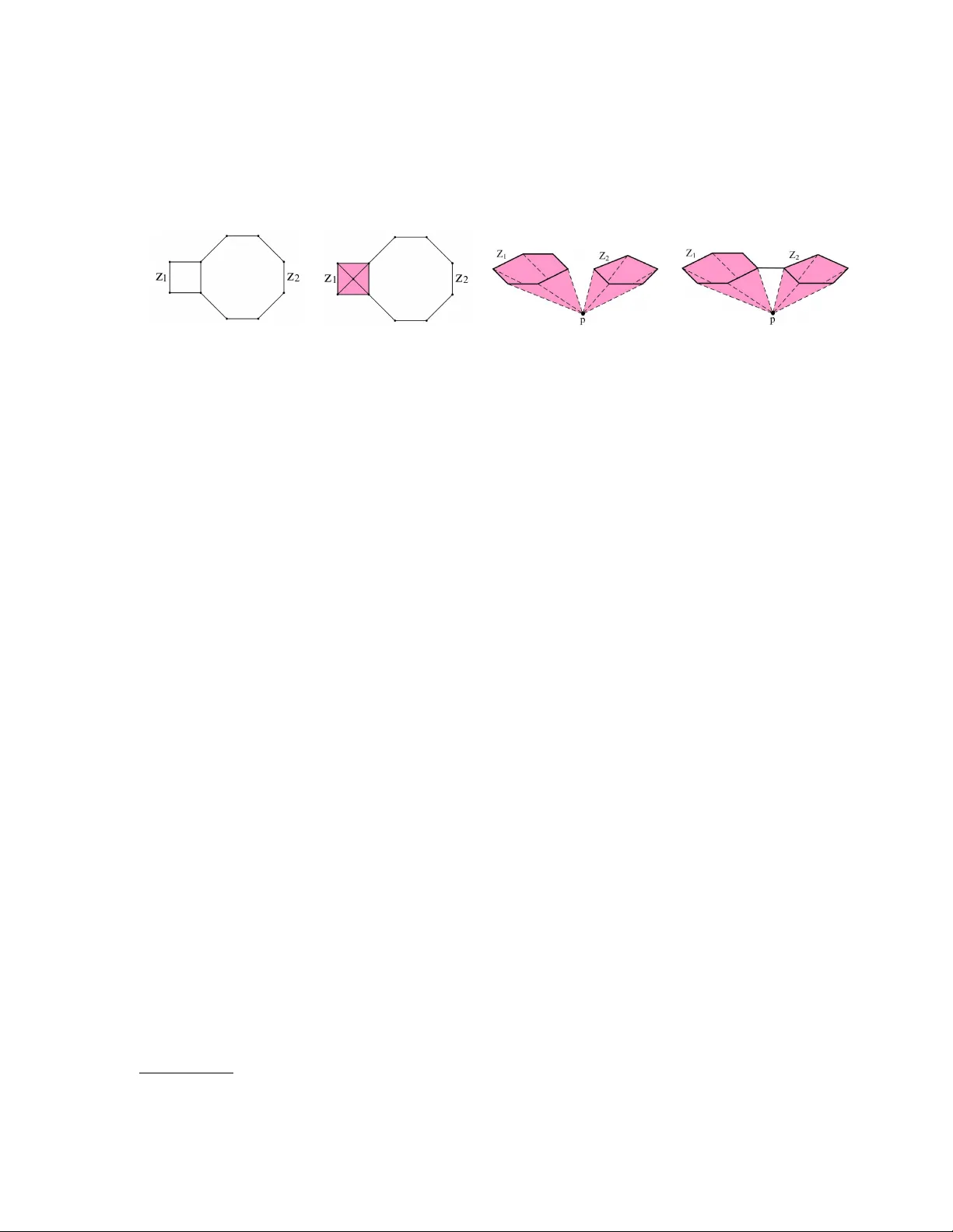
Symposium on Theoretical Aspects of Computer Science 2008 (Bordeaux), pp. 169-180 www .stacs-conf .org QUANTIFYING HOMOLOGY CLASSES CHAO CHEN 1 AND DANIEL FREEDMAN 1 1 Rensselaer P olytechnic Institu t e, 110 8th Street, T ro y , NY 12180, U.S.A. E-mail addr ess , { C. Chen, D. F reedman } : {chenc3, freedman} @cs.rpi.edu Abstra ct. W e develop a method f or mea suring homol ogy classe s. This inv olves three problems. First, w e define the size of a homology class, using ideas from relative homology . Second, w e d efine an optimal basis of a h omology group to b e the basis whose elements’ size hav e the minimal sum. W e provide a greedy algorithm to compute the optimal basis and measure classes in it. The algorithm runs in O ( β 4 n 3 log 2 n ) time, where n is the size of the simplicial complex and β is the Betti n umb er of the homology group . Third, we discuss d ifferent wa ys of lo calizing homology classes and prove some hardn ess results. 1. In tro duction The pr oblem of computing th e top ological features of a space has recent ly dra wn muc h atten tion fr om researc h er s in v arious fields, su c h as high-dimensional data analysis [3, 15], graphics [13, 5], net wo rk s [10] and computational biology [1, 8]. T op ological features are often preferable to purely geometric features, as they are more qualitativ e a nd global, and tend to b e more robust. If the goal is to characte rize a space, therefore, features which incorp orate topology seem to b e goo d candidates. Once w e are able to compute top ological f eatures, a natural p r oblem is to rank the features according to their imp ortance. The significance of this problem can b e justified from t wo p ersp ectiv es. First, un a v oidable errors are introd uced in data acquisition, in the form of traditional signal n oise, and finite s amp ling of con tinuous spaces. T hese errors ma y lead to the presence of man y small top ologic al features that are not “real”, but are simply artifacts of n oise or of samp ling [19]. Second, many problems are naturally hierarchical. This hierarch y – whic h is a kind of multiscale or multi-resolutio n decomp osition – implies that we wan t to capture the large scale features fi rst. S ee Figure 1(a) and 1(b) f or examples. The top ological features we use are h omology groups o v er Z 2 , due to their ease of computation. (Thus, throughout th is pap er, all the ad d itions are m o d 2 add itions.) W e w ould then lik e to quan tify or measure homo logy classes, as w ell as collections of classes. Sp ecifically , there are three problems we would lik e to solv e: (1) Measuring the size of a homology class: W e n eed a w ay to quan tify the size of a giv en homology class, and th is size measure should agree with intuition. F or example, in Figure 1(a), the m easure should b e able to distinguish the one large class (of the 1-dimensional homology group) from the t wo smaller classes. F u rthermore, 1998 ACM Subje ct C l assific ation: F.2.2, G.2.1. Key wor ds and phr ases: Compu t ational T op ology , Computational Geometry , Homolo gy , Persisten t Ho- mology , Localization, Op timization. c  Ch ao Chen and Daniel F reedman CC  Creative Comm on s Attribution-NoDe rivs License 170 CHAO CHEN AND DANIEL FREEDMAN (a) (b) (c) (d) Figure 1: (a,b) A disk with three holes and a 2- handled to rus are really more like a n a nn ulus and a 1- handled torus , resp ectively , b eca use the larg e features are mo re imp or tant. (c) A top ological spa ce formed fro m three cir cles. (d) In a disk with three holes , cycles z 1 and z 2 are well-loca lized; z 3 is no t. the measur e should b e easy to compute, and applicable to homology groups of an y dimension. (2) Cho osing a basis for a homology group: W e would lik e to c h o ose a “go o d” set of homology classes to b e the generators for the homology group (of a fi xed dimension). Su pp ose that β is the dimension of this group, and that we are usin g Z 2 co efficien ts; then there are 2 β − 1 nontrivial homology classes in total. F or a basis, we need to choose a su bset of β of these classes, sub ject to the constrain t that these β generate the group. The criterion of go o dness for a basis is based on an ov erall size m easure for th e basis, whic h relies in turn on the size measur e for its constituen t classes. F or instance, in Figure 1(c), we m ust c ho ose three from the seven nont r ivial 1-dimensional homology classes: { [ z 1 ] , [ z 2 ] , [ z 3 ] , [ z 1 ] + [ z 2 ] , [ z 1 ] + [ z 3 ] , [ z 2 ] + [ z 3 ] , [ z 1 ] + [ z 2 ] + [ z 3 ] } . In this case, the in tuitiv e c hoice is { [ z 1 ] , [ z 2 ] , [ z 3 ] } , as this c hoice reflects the fact that th er e is really only one large cycle . (3) Lo calization: W e need th e smallest cycle to repr esen t a homology class, giv en a natural criterion of the size of a cycle. The criterion should b e delib erately c hosen so that the corresp onding smallest cycle is b oth mathematically natur al and intu- itiv e. Su c h a cycle is a “well- lo calized” representat ive of its class. F or example, in Figure 1(d), the cycles z 1 and z 2 are we ll-lo calized rep resen tativ es of their r esp ectiv e homology classes; whereas z 3 is not. F urthermore, we mak e t wo add itional requirements on the solution of aforemen tioned prob- lems. Firs t, the solution ough t to b e compu table for top ological sp aces of arbitrary dimen- sion. Sec ond the solution should not require that the top ologic al space b e embedd ed, for example in a Euclidean space; and if th e space is em b edd ed, the solution sh ou ld not mak e use of the emb edding. These requir emen ts are natur al from the theoretical p oin t of view, but may also b e justified based on real applications. In mac hine learning, it is often assumed that the data lives on a manifold w hose dimension is muc h smaller than the dimension of the em b edding space. In th e study of shap e, it is common to enric h the sh ap e with other quan tities, s u c h as cur v ature, or color and other physical quanti ties. This leads to high dimensional m an if olds (e.g, 5-7 dimensions) em b edded in high dimensional am b ient spaces [4]. Although there are existing tec hn iques f or approac hin g the problems we hav e laid out, to our kno w ledge, there are no definitions and algo rith m s satisfying the t wo requiremen ts. Ordinary p ersistence [12, 20, 6] pro vides a measure of size, bu t only for those inessential QUANTIFYING HOMOLOGY CLASSES 171 classes, i.e. classes whic h ultimately d ie. More recen t w ork [7] attempts to remedy this situation, but not in an in tuitive w ay . Zomoro dian and C arlss on [21] use adv anced algebraic top ological mac hinery to solv e the basis co mp utation and lo calization p roblems. How ever, b oth the qu alit y of the result and th e complexity dep end strongly on the c hoice of the giv en co v er; th er e is, as y et, no suggestion of a canonical co ver. Other wo rk s lik e [14, 19, 11] are restricted to lo w dimension. Con tributions. In this pap er, w e solv e these problems. Ou r con tributions include: • Definitions of the size of homology classes and the optimal homology b asis. • A p ro v ably correct greedy algorithm to compu te the optimal homology b asis and measure its classes. This algorithm uses the p ersisten t homolog y . • An impro v ement of the str aightforw ard algorithm using fi nite fi eld linear alg ebr a. • Hardness r esults concerning the localization of homology classes. 2. Defining t he Problem In this section, we provide a tec hn iqu e for ranking h omology classes according to th eir imp ortance. Sp ecifically , we solv e the first tw o pr oblems mentio n ed in Section 1 b y formally defining (1) a meaningful s ize measure for h omology classes that is computable in arbitrary dimension; and (2) an optimal homology basis w hic h distinguishes large classes f r om small ones effec tivel y . Since we restrict our work to homology group s ov er Z 2 , when we talk ab out a d - dimensional chain, c , we refer to either a collect ion of d -simplices, or a n d -dimensional v ector ov er Z 2 field, whose non-zero entrie s corresp onds to the included d -simplices. n d is the num b er of d -dimensional simplces in the giv en complex, K . The r elev an t b ac kground in h omology and r elativ e homology can b e found in [16]. The Discrete Geo desic Distance. In order to m easure the size of homology classes, we need a notion of distance. As we w ill deal with a simplicial complex K , it is most natural to introd u ce a discrete metric, and corresp on d ing distance fun ctions. W e d efi ne the discr ete ge o desic distanc e f rom a vertex p ∈ v ert ( K ), f p : vert( K ) → Z , as follo ws. F or any v ertex q ∈ v ert( K ), f p ( q ) = dist( p, q ) is the length of the sh ortest path connecting p and q , in the 1-skel eton of K ; it is assu med that eac h ed ge length is one, though this can easily b e c hanged. W e ma y then extend this distance fu nction from vertic es to higher dimensional simplices naturally . F or any s implex σ ∈ K , f p ( σ ) is the maximal fun ction v alue of the v ertices of σ , f p ( σ ) = max q ∈ ve rt( σ ) f p ( q ). Finally , we d efine a discr ete ge o desic b al l B r p , p ∈ v ert( K ), r ≥ 0, as the su bset of K , B r p = { σ ∈ K | f p ( σ ) ≤ r } . It is straight forward to s ho w th at th ese sub sets are in fact sub c omplexes , namely , subsets that are s till sim p licial complexes. 2.1. Measuring the Size of a Homology Class W e start th is section by introdu cing n otions from relativ e homology . Giv en a simplicial complex K an d a su b complex L ⊆ K , we m a y wish to study the structur e of K b y ignoring all the chains in L . W e study th e gr oup of r elative chain as a quotient group, C d ( K, L ) = C d ( K ) / C d ( L ), whose elemen ts are r elative c hains . Analogous to the wa y we d efine the group of cycles Z d ( K ), the group of b oundaries B d ( K ) and the h omology group H d ( K ) in C d ( K ), w e 172 CHAO CHEN AND DANIEL FREEDMAN (a) (b) Figure 2: (a) On a disk with three holes , the three shaded r egions ar e the three smallest geodesic balls meas uring the three corr esp onding classes . (b) On a tub e, the sma lle st geo desic ball is c e n ter ed at q 2 , no t q 1 . define the gr oup of r elative cycles , the gr oup of r elative b oundaries and the r elative homolo gy gr oup in C d ( K, L ), denoted as Z d ( K, L ), B d ( K, L ) and H d ( K, L ), resp ectiv ely . W e denote φ L : C d ( K ) → C d ( K, L ) as th e homomorphism mapping d -c hains to their corresp ondin g relativ e c hains, φ ∗ L : H d ( K ) → H d ( K, L ) as the in duced homomorp hism mapping homology classes of K to their corresp onding relat ive h omology classes. Using these notions, w e define the size of a homology class as follo ws . Giv en a simplicial complex K , assu me we are giv en a collection of sub complexes L = { L ⊆ K } . F urth er m ore, eac h of these sub complexes is end o w ed with a size. In this case, we defin e the size of a homology class h as the size of the smallest L carrying h . Here we say a sub complex L c arries h if h has a trivial im age in the relativ e homology group H d ( K, L ), f orm ally , φ ∗ L ( h ) = B d ( K, L ). Intuitiv ely , this m eans that h disapp ears if we delete L from K , by con tracting it into a p oint and modd ing it out. Definition 2.1. The size of a class h , S ( h ), is the size of the smallest m easur able sub com- plex carryin g h , formally , S ( h ) = min L ∈L size( L ) suc h that φ ∗ L ( h ) = B d ( K, L ). W e say a sub complex L c arries a c hain c if L cont ains all the simplices of the c hain, formally , c ⊆ L . Usin g standard facts from algebraic top ology , it is straigh tforwa r d to see that L carries h if and only if it carries a cycle of h . Th is giv es us more intuition b ehind the measure definition. In this p ap er, we tak e L to b e the set of discr ete geo desic balls, L = { B r p | p ∈ v ert( K ) , r ≥ 0 } . 1 The size of a geo desic ball is n aturally its radius r . Th e smallest geod esic ball carrying h is denoted as B min ( h ) for con venience, wh ose r ad iu s is S ( h ). In Figure 2(a), the three geo desic balls cente red at p 1 , p 2 and p 3 are the smallest geod esic balls carrying non trivial homology classes [ z 1 ], [ z 2 ] and [ z 3 ], resp ectiv ely . Th eir radii are the size of the three classes. In Figure 2(b), the smallest geo desic ball carrying a n ontrivial h omology class is the pink one cen tered at q 2 , n ot the one cen tered at q 1 . Note that these geo desic balls ma y not look lik e Euclidean b alls in the em b edding space. 2.2. The O ptimal Homology Basis F or th e d -dimensional Z 2 homology group whose d imension (Betti n u mb er) is β d , there are 2 β d − 1 nontrivial homology classes. Ho wev er, w e only need β d of them to form a basis. 1 The id ea of grow ing geo desic discs has b een used in [19]. How ever, this w ork dep end s on lo w dimensional geometric reasoning, and h ence is restricted to 1-d imensional homology classes in 2-manifold. QUANTIFYING HOMOLOGY CLASSES 173 The basis shou ld b e c hosen wisely so th at we can easily d istinguish imp ortan t h omology classes f rom noise. S ee Figure 1(c) f or an example. T h ere are 2 3 − 1 = 7 nontrivial h omology classes; we need three of them to f orm a b asis. W e w ould prefer to c h o ose { [ z 1 ] , [ z 2 ] , [ z 3 ] } as a basis, rather than { [ z 1 ] + [ z 2 ] + [ z 3 ] , [ z 2 ] + [ z 3 ] , [ z 3 ] } . Th e former indicates that there is one big cycle in the top ological sp ace, wh ereas the latter giv es the impression of three large classes. In k eeping with this intuiti on, the optima l homolo gy b asis is defined as follo w s. Definition 2.2. The optimal homology b asis is th e basis for the homology group whose elemen ts’ size h a v e the minimal su m, f ormally , H d = argmin { h 1 ,...,h β d } β d X i =1 S ( h i ) , s.t. dim( { h 1 , ..., h β d } ) = β d . This definition guaran tees that large homology classes app ear as few times as p ossible in the optimal homology basis. In Figure 1(c), the optimal basis will b e { [ z 1 ] , [ z 2 ] , [ z 3 ] } , whic h has only one large class. F or eac h class in the basis, we need a cycle rep r esen ting it. As w e has sho wn, B min ( h ), the smallest geo desic ball carrying h , carries at lea st one cycle of h . W e lo calize eac h class in the optimal basis by its lo c alize d-cycles , whic h are cycles of h carried b y B min ( h ). Th is is a fair c hoice b ecause it is consisten t to th e size measure of h and it is computable in p olynomial time. See Section 5 for further discussions. 3. The Algor it hm In this section, we in tro duce an algorithm to compute the optimal homology b asis as defined in Defin ition 2.2. F or eac h class in the basis, w e measure its size, and r epresen t it with one of its lo calized-cycles. W e first introd uce an algorithm to compute the smallest homology class, namely , Measure -Smallest( K ) . Based on this p ro cedure, we p r o vide the algorithm Me asure-All( K ) , which computes the optimal homology basis. The algorithm tak es O ( β 4 d n 4 ) time, where β d is the Bet ti n u mb er for d -dimensional homology classes and n is the cardinalit y of the in put simp licial complex K . P ersisten t Homology . Our algorithm uses the p ersistent homology algorithm. In p ersis- ten t homology , we filter a top ologic al space with a scalar function, and capture the bir th and death times of homology classes of th e subleve l set du ring the filtration course. Classes with longer p ers istences are considered imp ortant ones. Classes with infin ite p ersistences are called essential homolo gy classes and corresp ond s to the int r insic h omology classes of the giv en top ologic al space. Please refer to [12, 20, 6] for theory and algorithms of p ersisten t homology . 3.1. C omputing the Smallest Homology Class The pr o cedure Measure -Smallest( K ) measures and lo calizes, h min , the smallest non- trivial homology class, namely , the one with the smallest size. Th e output of this pro cedure will b e a p air ( S min , z min ), n amely , the size and a lo calized-cycle of h min . Ac cordin g to the definitions, th is pair is d etermined by the sm allest geo desic ball carrying h min , namely , 174 CHAO CHEN AND DANIEL FREEDMAN B min ( h min ). W e fir st presen t the algorithm to compu te this ball. S econd, we explain ho w to compu te the pair ( S min , z min ) from the computed ball. Pro cedure Bm in( K ) : Computing B min ( h min ) . It is straight forward to see that the ball B min ( h min ) is also the smallest geo desic b all carrying any n on trivial homology class of K . It can b e compu ted by computing B r ( p ) p for all vertice s p , wh ere B r ( p ) p is the smallest geo desic ball cente red at p w hic h carries an y non trivial homology class. When all the B r ( p ) p ’s are computed, we compare their radii, r ( p )’s, and pic k the smallest b all as B min ( h min ). F or eac h v ertex p , we compu te B r ( p ) p b y applying the p ersisten t homology algorithm to K with the discrete geo desic distance from p , f p , as the filter function. Note that a geo desic ball B r p is the sublev el set f − 1 p ( −∞ , r ] ⊆ K . Non trivial homology classes of K are essentia l homology classes in th e p ersisten t homology algorithm. (In the rest of this pap er, w e ma y use “essent ial homology classes” and “non trivial h omology classes of K ” interc han gable.) Therefore, the birth time of the first essenti al homology class is r ( p ), and the su b complex f − 1 p ( −∞ , r ( p )] is B r ( p ) p . Computing ( S min , z min ) . W e compute the pair fr om the computed ball B min ( h min ). F or simplicit y , we den ote p min and r min as the ce nter and radius of the ball. According to the definition, r min is exactly the size of h min , S min . An y n on b ounding cycle (a cycle that is n ot a b oundary) carried b y B min ( h min ) is a localized-cycle of h min . 2 W e fir st computes a b asis for all cycles carried b y B min ( h min ), usin g a r eduction algorithm. Next, elemen ts in this basis are c hec k ed one b y one un til we find one w hic h is nounboun ding in K . T his c h ec king uses the algorithm of Wiedemann[18 ] for rank computation of sp arse matrices o ver Z 2 field. 3.2. C omputing the Optimal Homology Basis In this section, w e presen t the algorithm for computing the optimal homology b asis defined in Defin ition 2.2, namely , H d . W e fir st sho w that the optimal h omology basis can b e computed in a greedy manner. Second, we introdu ce an efficien t greedy algo r ith m . 3.2.1. Computing H d in a Gr e e dy Manner. Recall th at the op timal homology basis is the basis f or the homolog y group whose elemen ts’ size ha ve the minimal su m . W e use matroid theory [9 ] to sho w that we can compu te the optimal homology basis with a greedy m etho d. Let H b e the set of non trivial d -dimensional homology classes (i.e. the homology group min us the trivial class). Let L b e th e family of sets of linearly indep endent nontrivial homology classes. Then we ha ve th e follo wing th eorem, whose p ro of is omitted d ue to space limita tions. Th e same result has b een men tioned in [14]. Theorem 3.1. The p air ( H , L ) is a matr oid when β d > 0 . W e constru ct a we ighte d m atroid by assigning eac h nontrivia l homology class its size as the w eight . T his weig ht function is strictly p ositiv e b ecause a nontrivial homology cla ss can not b e carried by a geodesic ball with radiu s zero. According to matroid theory , we can compu te the optimal homology basis with a naive greedy metho d: c hec k the smallest non trivial homology classes one by one, until β d linearly indep end en t ones are collected. 2 This is true assuming that B min ( h min ) carries one and only one non trivial class, i.e. h min itself. How ever, it is straightforw ard to relax this assumption. QUANTIFYING HOMOLOGY CLASSES 175 The collecte d β d classes { h i 1 , h i 2 , ..., h i β d } form the optimal h omology basis H d . (Note that the h ’s are ord ered b y size, i.e. S ( h i k ) ≤ S ( h i k +1 ).) How eve r, th is method is exp on ential in β d . W e n eed a b etter solutio n . 3.2.2. Computing H d with a Se aling T e chnique. In this section, w e in tro d uce a p olynomial greedy alg orithm for computing H d . Instead of compu ting the smallest cla sses one b y one, our algorithm uses a sealing tec hniqu e and tak es time p olynomial in β d . Intuitiv ely , when the smallest l classes in H d are pic ked, w e mak e them trivial by add in g n ew simp lices to the giv en complex. In the augmented complex, an y linear com b inations of these pic ke d classes b ecomes trivial, and the s mallest n ontrivial class is th e ( l + 1)’th one in H d . The algorithm starts by measuring and lo calizing the smallest homology class of the giv en simplicial complex K (using the pro cedure Measure-Smallest( K ) introd uced in Sec- tion 3.1), which is also th e fi rst class we c h o ose for H d . W e mak e this class trivial by sealing one of its cycles – i.e. the lo calized-cycle we computed – with new simplices. Next, we measure and lo calize the smalle st h omology class of the augmen ted simplicial complex K ′ . This class is th e second smallest homology class in H d . W e mak e this class trivial again and pro ceed for the third smallest cla ss in H d . This p ro cess is rep eated f or β d rounds, yielding H d . W e mak e a homology class trivial b y sealing the class’s lo calized-cycle, w hic h w e ha ve computed. T o seal this cycle z , w e add (a) a n ew v ertex v ; (b ) a ( d + 1)-simplex for eac h d -simplex of z , with vertex set equ al to the ve rtex set of th e d -simplex tog ether with v ; (c) all of th e faces of these new simp lices. In Figure 3(a) and 3(b), a 1-cycle with four edges, z 1 , is sealed up with one new v ertex, four new triangles and four new edges. It is essen tial to make sure the new simplices do es not influence our measuremen t. W e assign the new ve r tices + ∞ geo desic distance f r om an y ve rtex in the original complex K . F urthermore, in the pro cedure M easure-Smallest( K ′ ) , we will n ot consid er an y geo desic ball cente r ed at these new ve r tices. In other w ord s, the geo desic distance from these new v ertices will nev er b e used as a filter function. Whenever we run the p ersistent homology algorithm, all of the new s im p lices ha ve + ∞ filter fu n ction v alues, f ormally , f p ( σ ) = + ∞ for all p ∈ v ert ( K ) and σ ∈ K ′ \ K . The algorithm is illustrated in Figure 3(a) an d 3(b). The 4-edge cycle, z 1 , and the 8-edge cycle, z 2 , are the lo calized-cycles of the smallest and the second smallest homology classes ( S ([ z 1 ]) = 2, S ([ z 2 ]) = 4). The n on b ounding cycle z 3 = z 1 + z 2 corresp onds to the largest n on trivial homology class [ z 3 ] = [ z 1 ] + [ z 2 ] ( S ([ z 3 ]) = 5). After the first round, we c ho ose [ z 1 ] as th e smallest class in H 1 . Next, we destro y [ z 1 ] by sealing z 1 , whic h yields the augmen ted complex K ′ . This time, w e c ho ose [ z 2 ], givi n g H 1 = { [ z 1 ] , [ z 2 ] } . Correctness. W e pro ve in Theorem 3.3 the correctness of our greedy metho d. W e b egin b y pro ving a lemma that d estro ying the smallest n on trivial class w ill neither destroy any other classes nor create an y new cla sses. P lease note that this is not a trivial result. The lemma do es not hold if w e seal an arbitrary class in stead of the smallest one. See Figure 3(c) and 3(d) for examples. Our pro of is based on the assumption that the smallest non trivial class h min is the only one carried b y B min ( h min ). Lemma 3.2. Given a simplicial c omplex K , if we se al its smal lest homolo gy c lass h min ( K ) , any other nontrivial homolo gy class of K , h , is stil l nontrivial in the augmente d simplicial c omplex K ′ . In other wor ds, any cycle of h is stil l nonb ounding in K ′ . 176 CHAO CHEN AND DANIEL FREEDMAN (a) (b) (c) (d) Figure 3: (a,b) the o riginal co mplex K and the augmented complex K ′ after destroying the smallest class, [ z 1 ]. (c) If the origina l co mplex K co nsists of the tw o cycles z 1 and z 2 , destroying a larger class [ z 1 ] + [ z 2 ] will make all other class es trivial to o . (d) The o riginal complex K consists o f the t wo cycles and an edg e connecting them. Destroying [ z 1 ] + [ z 2 ] will make all other classes trivial and cr eate a new class. This lemma leads to the correctness of our algorithm, namely , Theorem 3.3. W e pro ve this theorem by showing that the pro cedure Mea sure-All( K ) pr o duces the same result as the naiv e greedy algo r ithm. Theorem 3.3. The pr o c e dur e Me asure-All( K ) c omputes H d . 4. An Improv emen t Using Finite Field Linear A lgebra In this section, we present an impro v ement on the algorithm presen ted in the previous section, more sp ecifically , an impro vemen t on computing the s m allest geo desic b all carrying an y nontrivial class (the pr o cedure Bm in ). Th e id ea is b ased on th e fin ite field lin ear algebra b ehind the homology . W e fir st ob s erv e that for neighborin g v ertices, p 1 and p 2 , the birth times of the fi rst essen tial homology class using f p 1 and f p 2 as filter functions are close (Th eorem 4.1). This observ ation suggests that f or eac h p , ins tead of computing B r ( p ) p , we ma y just test w hether the geo desic b all cen tered at p with a certain radius carries an y essen tial h omology class. Second, with some algebraic ins ight, we reduce the prob lem of testing wh ether a geo desic ball carries an y essen tial homology cla ss to the p roblem of comparing dimensions of t wo vec tor spaces. F u rthermore, w e use Theorem 4.2 to redu ce the problem to rank computations of sparse m atrices on the Z 2 field, for which w e ha ve ready to ols from the literature. In what follo ws, w e assum e that K has a single comp onen t; m ultiple comp onen ts can b e accommodated with a s imple mo dification. Complexit y . In d oing so, we impro ve the complexit y to O ( β 4 d n 3 log 2 n ). More detailed complexit y analysis is omitted due to space limita tions. 3 Next, we present details of the impro vemen t. In Section 4.1, we pr o v e T h eorem 4.1 and pro vide details of the impr o v ed algorithm. In S ection 4.2, we explain ho w to test whether a certain su b complex carries an y essen tial homology class of K . F or con venience, in this section, w e use “carrying nonboun ding cycles” and “carrying essential homology classes” 3 This complexity is close to that of the p ersisten t homology algorithm, whose complexity is O ( n 3 ). Giv en the nature of the problem, it seems likely th at the p ersistence complexit y is a low er bound. I f this is the case, the current algorithm is nearly optimal. Cohen- Steiner et al.[8] provided a linear algorithm to maintai n the p ersistences while changing the filter function. While interesti n g, this algorithm is not applicable in our case. QUANTIFYING HOMOLOGY CLASSES 177 in terc h an geably , b ecause a geo desic ball carries essen tial homology classes of K if and only if it carries non b oun ding cycles of K . 4.1. The St abilit y of P ersistence Leads t o An Improv ement Cohen-Steiner et al.[6] prov ed that th e change, suitably d efined, of the p ersistence of homology classes is b ounded by the c hanges of the filter fun ctions. Since the fi lter fun ctions of t wo neigh b oring ve rtices, f p 1 and f p 2 , are close to eac h other, the birth times of th e first non b ounding cycles in b oth filters are close as well. This leads to Theorem 4.1. A simp le pro of is provided. Theorem 4.1. If two vertic es p 1 and p 2 ar e neighb ors, the birth times of the first non- b ounding cycles for filter fu nc tions f p 1 and f p 2 differ by no mor e than 1. Pr o of. p 1 and p 2 are neighbors implies that for an y p oin t q , f p 2 ( q ) ≤ f p 2 ( p 1 ) + f p 1 ( q ) = 1 + f p 1 ( q ), in wh ic h the in equalit y follo ws the triangular inequalit y . Th er efore, B r ( p 1 ) p 1 is a subset of B r ( p 1 )+1 p 2 . The form er carries nonb ounding cycles implies that the lat ter do es to o, and th u s r ( p 2 ) ≤ r ( p 1 ) + 1. Similarly , w e ha v e r ( p 1 ) ≤ r ( p 2 ) + 1. This theorem su ggests a wa y to a vo id computing B r ( p ) p for all p ∈ v ert( K ) in the pro cedur e Bmin . Sin ce our ob jectiv e is to find the minimum of th e r ( p )’s, we do a breadth- first searc h through all the vertic es with global v ariables r min and p min recording the smallest r ( p ) w e ha ve found and its corresp onding cent er p , resp ectiv ely . W e start by applying the p ersistent homology algorithm on K with filter function f p 0 , where p 0 is an arbitrary vertex of K . In itialize r min as the birth time of the first non b oundin g cycle of K , r ( p 0 ), and p min as p 0 . Next, w e do a breadth-fir s t searc h th rough th e rest vertice s. F or eac h ve r tex p i , i 6 = 0, there is a neighbor p j w e h a v e visited (the parent v ertex of p i in the breath-first searc h tree). W e kno w that r ( p j ) ≥ r min and r ( p i ) ≥ r ( p j ) − 1 (T h eorem 4.1). Therefore, r ( p i ) ≥ r min − 1. W e only need to test whether the geo desic b all B r min − 1 p i carries an y nonb ounding cycle of K . If so, r min is decremen ted by one, and p min is up dated to p i . After all ve rtices are visited, p min and r min giv e us the ball w e w an t. Ho w eve r , testing whether the sub complex B r min − 1 p i carries an y nonb ounding cycle of K is not as easy as computing n onb ounding cycles of the s ub complex. A n onb ounding cycle of B r min − 1 p ma y n ot b e non b ounding in K as we require. F or example, in Figure 4(a) and 4(b), the simplicial complex K is a toru s with a tail. The p ink geo desic ball in the first figure do es not carry any n on b ounding cycle of K , although it carries its o wn n on b ounding cycles. The geo desic ball in the second figure is the one that carries non b ound ing cycles of K . Therefore, we need algebraic to ols to distinguish nonboun ding cycles of K from those of the sub complex B r min − 1 p i . 4.2. Pro cedure Co ntain-Nonb oundin g-Cycle : T esting Whether a Sub complex Car- ries Non b ounding Cycles of K In this section, we presen t the pro cedur e for testing whether a sub complex K 0 carries an y nonb ounding cycle of K . A c hain in K 0 is a cycle if and only if it is a cycle of K . Ho w eve r , solely fr om K 0 , we are not able to tell w hether a cycle carried by K 0 b ound s or not in K . Instead, we wr ite the set of cycles of K carried by K 0 , Z K 0 d ( K ), and the set of 178 CHAO CHEN AND DANIEL FREEDMAN (a) (b) (c) (d) Figure 4: (a,b) I n a torus with a tail, only the ball in the seco nd fig ure carr ies nonbounding cycles of K , although in b oth figures the balls hav e no nt r ivial top ology . (c,d) The cycles with the minimal ra dius and the minimal diameter, z r and z d (Used in Section 5). b ound aries of K carried by K 0 , B K 0 d ( K ), as sets of linear com binations with certain con- strain ts. Consequen tly , we are able to test whether any cycle carried by K 0 is n on b ounding in K by comparing their dimens ions . F ormally , w e define B K 0 d ( K ) = B d ( K ) ∩ C d ( K 0 ) and Z K 0 d ( K ) = Z d ( K ) ∩ C d ( K 0 ). Let ˆ H d = [ z 1 , ..., z β d ] b e the matrix whose column v ectors are arbitrary β d non b ounding cycles of K which are not h omologous to eac h other. Th e b ou n dary group and the cycle group of K are column spaces of the matrices ∂ d +1 and ˆ Z d = [ ∂ d +1 , ˆ H d ], resp ectiv ely . Using finite field linear algebra, we hav e th e follo w ing theorem, wh ose pro of is omitted du e to space limita tions. Theorem 4.2. K 0 c arries nonb ounding cycles of K if and only if rank( ˆ Z K \ K 0 d ) − rank( ∂ K \ K 0 d +1 ) 6 = β d . wher e ∂ i d +1 and ˆ Z i d ar e the i - th r ows of the matric es ∂ d +1 and ˆ Z d , r esp e ctively. W e use th e algorithm of Wiedemann[18] for the rank compu tation. In our algorithm, the b oundary matrix ∂ d +1 is give n . The matrix ˆ H d can b e precomputed as follo ws. W e p erform a column reduction on the b oun dary matrix ∂ d to compute a basis for the cycle group Z d ( K ). W e c hec k elemen ts in this b asis one b y one u n til we collect β d of them f orming ˆ H d . F or eac h cycle z in this cycle basis, w e c h ec k whether z is linearly indep en den t of the d -b oundaries and the n on b ounding cycles w e ha ve already c hosen. More d etails are omitted due to space limitat ions. 5. Lo calizing Classes In this section, we address the lo caliza tion problem. W e formalize the lo calizati on problem as a com b in atorial optimizatio n p roblem: Giv en a simplcial complex K , compute the represen tativ e cycle of a given homolo gy class minimizing a certain ob jectiv e function. F ormally , giv en an ob jectiv e function defined on all the cycles, cost : Z d ( K ) → R , w e w ant to lo calize a give n class with its optimal ly lo c alize d cycle , z opt ( h ) = argmin z ∈ h cost( z ). In general, w e assum e the class h is giv en by one of its represen tativ e cycles, z 0 . W e explore th ree options of the ob jectiv e function cost( z ), i.e. the volume , diameter and r adius of a giv en cycle z . W e sho w that the cycle w ith the m inimal volume and the cycle with the minimal diameter are NP-h ard to compu te. Th e cycle with the minimal radius, QUANTIFYING HOMOLOGY CLASSES 179 whic h is the lo calized-cycle we defi n ed and computed in previous sections, is a fair c h oice. Due to space limitati ons, we omit pro ofs of theorems in this section. Definition 5.1 (V olume) . Th e vo lum e of z is the n umb er of its simplices, vol( z ) = card( z ). F or example, the v olume of a 1-dimensional cycle, a 2-dimensional cycle and a 3- dimensional cycle are th e num b ers of their ed ges, triangles and tetrahedra, resp ectiv ely . A cycle with the s mallest volume, denoted as z v , is consisten t to a “w ell-localized” cycle in intuitio n. Its 1-dimensional version, the shortest cycle of a class, has b een studied by researc hers [14, 19, 11]. How ever, we p ro ve in Theorem 5.2 that computing z v of h is NP- hard. 4 The p ro of is by reduction from the NP-hard problem MAX-2SA T-B [17]. More generally , we can extend the the v olume to b e th e sum of the w eigh ts assigned to simplices of the cycle, give n an arb itrary w eigh t fu nction defi n ed on all the simplices of K . T he corresp ondin g smallest cycle is still NP-hard to co mp ute. Theorem 5.2. Computing z v for a g i ven h is NP- har d. When it is NP-hard to compute z v , one ma y resort to the geo desic distance b etw een elemen ts of z . The seco n d c hoice of the ob j ectiv e fu nction is the d iameter. Definition 5.3 (Diameter) . The d iameter of a cycle is the diameter of its v ertex set, diam( z ) = diam(v ert( z )), in wh ich the diameter of a set of ve rtices is the maximal geo desic distance b etw een them, formally , diam( S ) = max p,q ∈ S dist( p, q ). In tuitivel y , a repr esen tativ e cycle of h with the minimal diameter, denoted z d , is the cycle wh ose vertic es are as close to eac h other as p ossible. Th e int u ition will b e furth er illustrated by comparison against the r adius criterion. W e p ro ve in Th eorem 5.4 that com- puting z d of h is NP-hard, b y reduction from the NP-hard Multiple-Choic e Cover Pr oblem (MCCP) of Arkin and Hassin [2]. Theorem 5.4. Computing z d for a given h is NP- har d. The third option of the ob j ectiv e function is the radius. Definition 5.5 (Radiu s) . Th e radius of a cycle is th e radius of the smallest geo desic ball carrying it, formally , rad( z ) = min p ∈ vert( K ) max q ∈ ve rt( z ) dist( p, q ), where v ert ( K ) and v ert ( z ) are the sets of vertic es of the give n simplicial complex K and the cycle z , resp ectiv ely . The represent ativ e cycle with the minimal radius, denoted as z r , is the same as the lo calized-cyc le defined and compu ted in previous sections. In tuitive ly , z r is the cycle whose v ertices are as close to a vertex of K as p ossible. Ho wev er, z r ma y not necessarily b e lo calized in intuition. It ma y wiggle a lot while still b eing carried by the smallest geod esic ball carrying the class. See Figure 4(c), in whic h w e lo calize th e only nontrivia l homology class of an ann ulu s (the light gra y area). T he dark gra y area is the smallest geod esic ball carrying the cla ss, whose cen ter is p . Besides, the cycle with the minimal diameter (Fi gur e 4(d)) a vo ids this wiggling problem and is concise in in tuition. T h is in turn justifies th e c hoice of diameter. 5 W e can pr ov e that z r can b e computed in p olynomial time and is a 2-appro ximation of z d . 4 Eric kson and Whittlesey [14] lo calized 1-dimensional classes with their shortest represen tative cycles. Their p olynomial algorithm can only lo calize classes in th e shortest homology basis, not arbitrary given classes. 5 This figure also illustrates that the radius and t he diameter of a cycle are not strictly related. F or the cycle z r in the left, its diameter is twice of its radius. F or the cycle z d in the center, its diameter is equal to its radius. 180 CHAO CHEN AND DANIEL FREEDMAN Theorem 5.6. We c an c ompute z r in p olynomial time. Theorem 5.7. diam( z r ) ≤ 2 diam( z d ) . This b ound is a tigh t b oun d . In Figure 4(c) and 4(d), the diameter of the cycle z r is t wice of the radius of the dark gray geod esic b all. The d iameter of the cycle z d is the same as the radius of the ball. W e ha ve diam( z r ) = 2 diam( z d ). Ac knowled gemen t s The authors wish to ackno wledge constru ctive commen ts from anonymous r eview ers and fruitful discussions on p ersisten t homology with Professor Herbert Edelsbrun ner. References [1] P . K. Agarw al, H. Ed elsbrunner, J. Harer, and Y. W ang. Extreme elev ation on a 2-manifold. Discr ete & Computational Ge ometry , 36:553–57 2, 2006. [2] E. M. Ark in and R. Hassin. Minimum-diameter cover ing problems. Networks , 36(3):147–155, 2000. [3] G. Carlsson. Pers istent homology and the analysis of high d imensional data. Symp osium on the Geom- etry of V ery Large Data Sets, F ebrary 2005. Fields Institute for Research in Mathematical Sciences. [4] G. Carlsson, T. Ishkhanov, V. de Silv a, and L. J. Gu ibas. Persis ten ce barco des for shapes. International Journal of Shap e M o deli ng , 11(2):149–188, 2005. [5] C. Carner, M. Jin, X. Gu, and H. Qin. T opology-driven surface mapp ings with robust feature alignment. In I EEE Visualization , p. 69, 2005. [6] D. Cohen-Steiner, H. Edelsbrunner, and J. Harer. Stability of p ersistence diagrams. Discr ete & Com- putational Ge ometry , 37:103–1 20, 200 7. [7] D. Cohen-Steiner, H. Edelsbrunner, and J. H arer. Ex tending p ersistent homology using Poincar ´ e and Lefsc hetz duality . F oundations of Computational Mathematics , to app ear. [8] D. Cohen-Steiner, H. Edelsbrunner, and D. Morozo v. Vines and vineyards by up dating p ersistence in linear time. In Symp osium on Computational Ge ometry , pp. 119–126, 2006. [9] T. H . Cormen, C. E. Leiserson, R. L. Rivest, and C. S tein. Intr o duction to Algorithms. MIT Press, 2001. [10] V. de Silv a and R. Ghrist. Cov erage in sensor netw orks via p ersistent homology . Algebr aic & Ge ometric T op ol o gy , 2006. [11] T. K. D ey , K. Li, and J. S un. On compu ting handle and tunn el lo ops. In IEEE Pr o c. NASAGEM , 2007. [12] H. Edelsbrunner, D. Letscher, and A. Zomoro dian. T op ological p ersistence and simplification. Di scr ete & Computational Ge ometry , 28(4):511–53 3, 2002. [13] J. Erickson and S. Har-Peled. Optimally cutt ing a surface in to a disk. Discr ete & Computational Ge- ometry , 31(1):37–59, 2004. [14] J. Erickson and K. Wh ittlesey . Greedy optimal h omotop y and homology generators. I n SODA , pp . 1038–10 46, 2005. [15] R. Ghrist. Barco des: t h e p ersistent top ology of data. A mer. Math. So c Current Even ts Bulletin. [16] J. R. Munk res. Elements of Algebr aic T op olo gy. Ad dison-W esley , Redwook Cit y , California, 1984. [17] C. Papadimitrio u and M. Y ann ak akis. O ptimization, app ro x imation, and complexity classes. In Pr o c. 20th ACM Symp osium on The ory of c omputing , pp . 229–234, New Y ork, N Y, US A, 1988. ACM Press. [18] D. H . Wiedemann. Solving sparse linear equations o ver fin ite fields. IEEE T r ansactions on Information The ory , 32(1):54–62, 1986. [19] Z. J. W oo d, H . Hopp e, M. Desbru n, an d P . S chr¨ oder. Removing excess top ology from isosurfaces. A CM T r ans. Gr aph. , 23(2):190–208, 2004. [20] A. Zomorodian and G. Carlsson. Computing p ersisten t homology . Di scr ete & Computational Ge ometry , 33(2):249– 274, 2005. [21] A. Zomorodian and G. Carlsson. Lo calized homology . In Shap e Mo deli ng International , pp. 189–198 , 2007. This work is licensed under t he Cr eative Commons Attribution-No Derivs Licens e. T o view a copy of this license, visit http:/ /creativ e commons.org/licenses/by- n d/3.0/ .