The normal distribution in some constrained sample spaces
Phenomena with a constrained sample space appear frequently in practice. This is the case e.g. with strictly positive data and with compositional data, like percentages and the like. If the natural measure of difference is not the absolute one, it is…
Authors: G. Mateu-Figueras, V. Pawlowsky-Glahn, J.J. Egozcue
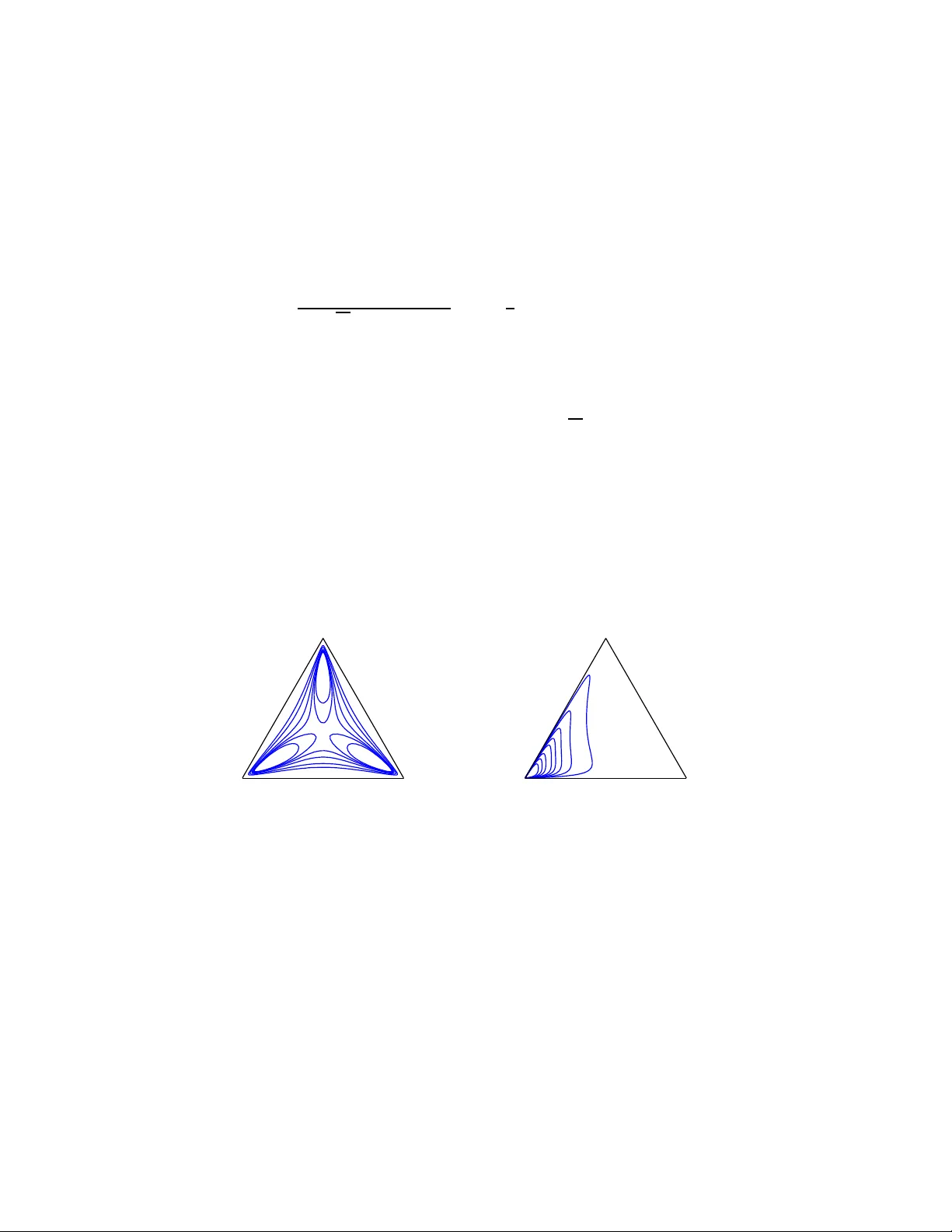
The normal distrib ution in some constrai ned sample spaces G. Mateu-Figueras Universitat de Girona, Girona, Spain . V . P a wlo wsky-G lahn Universitat de Girona, Girona, Spain . J.J . Egozc ue Universitat P olit ´ ecnica de Catalunya, Barcelona, Spain. Summary . Phenome na with a constr ained sample spa ce appear frequ ently in practice. This is the case e.g. with stri ctly positi v e data and with compositio nal data, like percentag es and the lik e. If the natural measure of difference is not th e absolut e on e, i t is possible to use simpl e algeb raic prope r ties to show tha t it is more conv enien t to work wi th a geometr y that is no t the usual Euclidea n geometr y in real space, and with a measure which is not the usua l Lebesgue measure, leadi ng to alte rn ative models which better fit the phen omenon u nder study . T he general app roach is presen ted and i llustrated both on the p ositive real lin e and on the D -par t simplex. K eyw ords : L ognor mal; Additive logistic nor mal. 1. Introduction In gener al, an y statistical a nalysis is p erfor med ass uming data to be r ealisations of rea l random vectors whos e density functions are defined with r esp ect to the Lebesg ue mea- sure, which is a natural m easure in real space and compatible with its inner vector space structure. Sometimes, like in the case of observ ations measured in per centages, random vectors ar e defined o n a constrained sample spa c e, E ⊂ R D , and metho ds and conce pts used in real spa ce lea d to absurd re s ults, as it is well known from exa mples like the spurious co rrelations betw een pro po rtions (Pearson, 1897). This pr oblem ca n be circum- ven ted when E admits a meaningful Euclidean space s tructure different from the usual one (Pa wlo wsky and Ego zcue, 20 01). In fact, if E is an Euclidea n space, a mea sure λ E , compatible with its str ucture, is o bta ined from the Leb esg ue measur e on o r thonormal co or- dinates (Eaton, 1 983; P awlo wsky-Glahn, 2 003). Then, a probabilit y densit y function, f E , is defined on E as the R adom-Niko d´ ym derivative of a probability measure P with re spe ct to λ E . The measure λ E has prop erties comparable to those of the Leb esgue measur e in real space. Difficulties, arising from the fact that the integral P( A ) = R A f E ( x ) dλ E ( x ) is not a n ordina ry one, are so lved working with coor dinates (Eaton, 19 83), and in pa rticular working with co ordinates with r e spe c t t o an orthonormal b asis (P awlo ws ky-Glahn, 200 3), as proper ties that hold in the space of co ordinates transfer directly to the spa c e E . F o r example, for f E a density function on E , call f the density function o f the co ordina tes, and then the proba bilit y of an even t A ⊆ E is computed as P( A ) = R V f ( v ) dλ ( v ) , where V and v are the representation of A a nd x in terms of the orthonormal coordina tes c hosen, and 2 G. Mateu-Figu eras, V . Pa wlowsky-Glahn and J .J. Egozcue λ is the Leb esgue measure in the space of co or dinates. Using f to compute any element of the sample spa ce, e.g. the exp ected v a lue, the co ordinates of this element with resp ect to the s ame orthonor mal basis are obtained. The corres p onding element in E is then given b y the repres en tation o f the element in the basis. Every o ne-to-one transfor mation b et ween a set E and re a l space induces a rea l Eu- clidean space structure in E , with ass o ciated measure λ E . Particularly interesting ar e those transfor mations related to the measure o f differ ence b etw e en observ a tions, as ev i- denced by Ga lton (187 9) when introducing the logarithmic tr ansformation as a mea n to ackno wledge F echner’s law, acco rding to which p er c eption e quals lo g(stimu lu s) , formalise d by McAlister (18 79). This simple appro ach has acquired a growing imp ortance in a pplications, since it has bee n recog nised that many c onstr aine d sample sp ac es , which are subs ets of so me real spa ce— like R + or the simplex—can b e str uctured as Euclidean vector s pa ces (Pawlo wsky and Egozc ue, 200 1). It is imp ortant to empha s ise that this approach implies using a measure which is different from the usual Leb esgue measure. Its a dv antage is that it op ens the door to alternative statistical mo dels dep ending not only on the assumed dis tribution, but a lso on the measure which is consider ed a s appropr ia te or na tural for the studied phenomenon, thus enhancing int erpretation. The idea of using not only the appropriate spac e structure, but also to change the measure, is a p ow erful to ol b ecause it leads to results coherent with the interpretation of the measure o f difference, and b ecause they a re mathematically mor e straightforward. 2. Pr obability densities in Euclidea n vector spaces Let E ⊆ R D be the sa mple spa c e for a ra ndom vector X , i.e. each re alization of X is in E . Assume that there exists a one-to-o ne differenciable mapping h : E → R d with d ≤ D . This mapping allows to define a Euclidea n structure on E just trans la ting the standar d prop erties of R d int o E . The exis tence o f the mapping h implies s o me characteristics o f E . An imp or tant one in this context is that E must hav e some bo rder set so that h tr ansforms neighborho o ds of this bor de r into neighbor ho o ds of infinit y in R d . F or ins ta nce, a sphere in R 3 with a defined po le c a n b e trans fo rmed into R 2 , but, if no po le is defined, this is no longer p ossible. The inner sum ⊕ and the o uter pro duct ⊙ in E are defined as x ⊕ y = h − 1 ( h ( x ) + h ( y )) , α ⊙ x = h − 1 ( α · h ( x )), where x , y are in E and α ∈ R . With these defini- tions E is a vector space of dimension d . The metric s tr ucture is induced b y the in- ner pro duct h x , y i E = h h ( x ) , h ( y ) i , whic h implies the norm a nd the dis tance k x k E = k h ( x ) k , d E ( x , y ) = d( h ( x ) , h ( y )), thus co mpleting the Euclidean structure of E , bas ed on the inner pro duct, norm and dis tance in R d , denoted as h· , ·i , k · k , d( · , · ) resp ectively . By con- struction, h ( x ) is the vector of co o rdinates of x ∈ E . The co ordinates c orresp ond to the or- thonormal basis in E g iven by the images o f the canonic a l ba sis in R d by h − 1 . The Leb esg ue measure in R d , λ d induces a mea sure in E , deno ted λ E , just defining λ E ( h − 1 ( B )) = λ d ( B ), for any Bor elian B in R d . In order to define p df ’s in E , a reference measure is needed. When E is viewed as a subset o f R D , the Leb esgue measur e , λ D , can b e even tually used. Howev er , if d < D the random vector X canno t b e absolutely contin uous with resp ect to λ D . Our prop o s al, and a more natural way to define a p df for X , is to s tart with a p df for the (ra ndom) co or dina tes Y = h ( X ) in R d . Assume that f Y is the p df o f Y with resp ect to the Leb esgue measure, λ d , in R d , i.e. Y is a bsolutely contin uous with resp ect to λ d and the p df is the Radom- Nik o d´ ym The nor mal distri bution in some constrained sample spaces 3 deriv ative f Y = dP /dλ d . The random vector X is recovered fro m Y a s X = h − 1 ( Y ) but, when D > d , h − 1 can b e restricted to only d of its comp onents; let h − 1 d be s uch a restrictio n and X d = h − 1 d ( Y ). The inv er se mapping is denoted by h d ( X d ) = h ( X ). This means that mor e tha n d comp onents result in a r e dundant definition of X . When D = d , the restrictio n of h − 1 reduces to the ident ity h − 1 = h − 1 d . The pdf of X d with resp ect to the Leb e sgue measure in R d is computed using the Jacobian rule f X d ( x d ) = dP dλ d ( x d ) = f Y ( h d ( x d )) · ∂ h d ( x d ) ∂ x d , (1) where the last ter m is the d -dimensiona l J acobian of h d . The next step is to e xpress the p df with resp ect to λ E , the natural measure in the sample space E . The chain rule for Ra dom-Nikod´ ym deriv atives implies f E X d ( x d ) = dP dλ E ( x d ) = dP dλ d ( x d ) · dλ d dλ E ( x d ) , (2) and the last deriv ative is dλ d dλ E ( x d ) = ∂ h − 1 d ( h d ( x d )) ∂ y = ∂ h d ( x d ) ∂ x d − 1 , (3) due to the inv erse function theorem. Substituting (2) and (3) into (1), f E X ( x ) = dP dλ E ( x ) = f Y ( h ( x )) , (4) where the subscripts d have b een suppressed b ecause they only play a ro le when computing the J a cobians. The representation of random v a r iables b y pdf ’s defined with resp ect to the measure λ E requires a r eview of the moments and other c haracteris tics o f the p df ’s . F ollowing Eaton (1983), the exp ectation and v ariance of X c a n b e defined as follows. Let X b e a random v ariable supp orted on E and h : E → R d the coo rdinate function defined o n E . The e x pec ta tion in E is E E [ X ] = Z ⊕ E x f E X ( x ) d x = h − 1 Z R d y f h ( X ) ( y ) d y (5) = h − 1 (E[ h ( X )]) , (6) provided the integrals ex ist in the Leb esgue sense. This definition des erves some remark s. The first integral in (5) has b een sup erscr ipted with ⊕ b ecaus e the inv olved s um is ⊕ fo r elements in E . The pra ctical way to carry o ut the integral is to r epresent the elements of E using co ordinates and to integrate us ing the p df o f the co or dinates; the r esult is transfor med back into E . Finally , (6) summar izes the previous equation using the standard definition of exp ectation of the co or dinates in R d . V ariance in volv es only real exp ectations and can b e identified with v a riance of co o r- dinates. Specia l attention deserves the metric v a r iance or to tal v ariance (Aitchison, 1 9 86; Pa wlowsky a nd Ego zcue, 20 0 1). Assuming the exis tence o f the int egrals , metric v a riability 4 G. Mateu-Figu eras, V . Pa wlowsky-Glahn and J .J. Egozcue of X with res pec t to a po int z ∈ E ca n be defined as V ar [ X , z ] = E[d 2 E ( X , z )] . The minimum metric v ariability is attained fo r z = E E [ X ], th us s upp or ting the definition (5)–(6). The metric v aria nce is then V ar[ X ] = E [d 2 E ( X , E E [ X ])] . (7) The mo de o f a p df is normally defined a s its maximum v a lue, althoug h lo ca l maxima are normally also called mo des. How ev er, the shap e and, pa rticularly , the max im um v alues depe nd on the reference measure taken in the Radom-Nikod ´ ym der iv atives of the density . Since the Le bes g ue mea sure in the c o ordinate s pa ce, R d , cor resp onds to the measur e λ E , the mo de can b e defined as Mo de E [ X ] = arg ma x x ∈ E { f E X ( x ) } = h − 1 argmax y ∈ R d { f h ( X ) ( y ) } , where the usual r emarks on multiple mo des or a symptotes are in order. 3. The positive real line The real line, with the ordinary sum a nd pr o duct by scala rs, has a vector space str uc- ture. The ordinar y inner pro duct a nd the Euclidean distance ar e co mpatible with these op erations. But this g eometry is not s uitable for the po sitive real line. Confront, for ex- ample, some meteoro logists with tw o pairs of samples taken at t wo rain gauges, { 5 ; 10 } and { 100 ; 105 } in mm, and ask for the difference; quite probably , in the firs t ca se they will say there was do uble the total r ain in the seco nd gaug e compar ed to the first, while in the second ca se they will say it rained a lot but approximately the s ame. They a re as suming a relative measure of difference. As a result, the na tural measure of difference is not the usua l Euclidean one and the ordinar y vector spa ce str ucture of R do e s not b e hav e suitably . In fact, pr oblems might app ear shifting a p ositive num ber (vector) by a negative r eal num ber (vector); or multiplying a positive num ber (vector) by an arbitrar y r eal num ber (scalar), bec ause results can b e outside R + . There are tw o ope r ations, ⊕ , ⊙ , which induce a vector space str ucture in R + (Pa wlo wsky a nd Ego zcue, 20 01). In fact, given x, y ∈ R + , the in ternal op eratio n, which plays an analo gous ro le to additio n in R , is the usual pro duct x ⊕ y = x · y and, for α ∈ R , the external op er ation, which plays an a nalogous role to the pro duct by s calars in R , is α ⊙ x = x α . An inner pr o duct, compatible with ⊕ and ⊙ is h x, y i + = ln x · ln y , whic h induces a no rm, k x k + = | ln x | , and a distance, d + ( x, y ) = | ln y − ln x | , and thus the co mplete Euclidean space structur e in R + . Since R + is a 1-dimensio nal vector space there are o nly tw o or thonormal basis: the unit-vector ( e ) and its inv erse element with res pec t to the internal op eration ( e − 1 ). F rom now o n the fir st o ptio n is consider ed a nd it will b e denoted by e . Any x ∈ R + can be expressed as x = ln x ⊙ e = e ln x which re veals that h ( x ) = ln x is the co o rdinate of x with res pect to the basis e . The measur e in R + can b e defined so that, for an interv al ( a, b ) ⊂ R + , λ + ( a, b ) = λ (ln a, ln b ) = | ln b − ln a | and dλ + /dλ = 1 /x (Mateu-Figuera s, 20 0 3; Pa wlowsky-Glahn, 2003). F ollowing the notation in Section 2, a ll these definitions can b e obtained by setting E = R + , D = d = 1 and h ( x ) = ln x . The g eneralizatio n to E = R D + is straightforward: for x ∈ R D + , the co ordina te function can be defined as h ( x ) = ln ( x ), where the loga r ithm applies comp onent-wise. 3.1. The normal distr ibu tion on R + Using the alg ebraic-g eometric structure in R + and the measure λ + , the norma l distribution on R + is defined by Mateu- Fig ueras et.at. (200 2) through the density function of orthonor - The nor mal distri bution in some constrained sample spaces 5 mal co ordinates. Definition 1. Le t b e (Ω , F , P ) a proba bility s pace. A r andom v ar iable X : Ω − → R + is said to hav e a normal on R + distribution with tw o par ameters µ and σ 2 , written N + ( µ, σ 2 ), if its density function is f + X ( x ) = dP dλ + ( x ) = 1 √ 2 π σ exp − 1 2 (ln x − µ ) 2 σ 2 , x ∈ R + . (8) The density (8) is the usua l nor ma l density applied to co ordina tes ln x as implied by (4) and it is a density in R + with resp ect to the λ + measure. This density function is completely restricted to R + and its expr ession corr esp onds to the law of frequency introduced by McAlister (1879). The contin uo us line in Fig.1 represents the de ns it y function (8) for µ = 0 and σ 2 = 1 . 0 0.5 1 1.5 2 2.5 3 3.5 4 0 0.1 0.2 0.3 0.4 0.5 0.6 0.7 Fig. 1. Densit y functio ns Λ (0 , 1) (- - - -) and N + (0 , 1) (——). According to this approa ch, the normal distribution in R + exhibits the same c harac- teristics as the nor mal distribution in R , the mos t relev an t of which are summarized in the following prop er ties . A complete pro of of the following prop erties is pr esented in the app endix. Pr op ert y 1. Let b e X ∼ N + ( µ, σ 2 ), and consta n ts a ∈ R + and b ∈ R . Then, the ra ndom v aria ble X ∗ = a ⊕ ( b ⊙ X ) = a · X b is distributed as N + (ln a + bµ, b 2 σ 2 ). Pr op ert y 2. Let be X ∼ N + ( µ, σ 2 ) a nd a ∈ R + . Then, f + a ⊕ X ( a ⊕ x ) = f + X ( x ),where f + X and f + a ⊕ X represent the probability density functions of the random v a riables X and a ⊕ X = a · X , res pectively . Pr op ert y 3. If X ∼ N + ( µ, σ 2 ), then E + [ X ] = Med + [ X ] = Mo de + [ X ] = e µ . Pr op ert y 4. If X ∼ N + ( µ, σ 2 ), then V ar [ X ] = σ 2 . Notice that Pr o p e r ty 1 implies that the family N + ( µ, σ 2 ) is closed under the op eratio ns in R + and Pr op erty 2 a sserts the inv a riance under translations in R + . The exp ected v alue, the media n and the mode a re elements of the suppo rt space R + , but the v a riance is only a numerical v alue which describ es the disp ersio n of X . W e a re used to take the square ro ot of σ 2 as a wa y to r epresent interv als centered a t the mean and with radius equal to some standar d deviations . T o o btain s uc h an interv al centered at 6 G. Mateu-Figu eras, V . Pa wlowsky-Glahn and J .J. Egozcue E[ X ] = e µ with length 2 k σ , take ( e µ − kσ , e µ + kσ ) as d + ( e µ − kσ , e µ + kσ ) = 2 k σ . This kind o f int erv al is used in practice (Ahre ns , 1 954) and predictive interv als in R + taking exp onential of predictive in terv als co mputed from the log-transfor med data under the hypothesis of normality ar e obtained. In Fig .2(a) we repr esent the interv al ( e µ − σ , e µ + σ ) for a N + ( µ, σ 2 ) density function with µ = 0 and σ 2 = 1. It can b e shown that it is of minimum length, and it is also an iso densit y in terv al thus, the distribution is symmetric around e µ . This symmetry might seem par adoxical, as one ca nnot see it in the sha pe of the density function. But still, it is symmetric within the linear vector space structure of R + , a lthough cer tainly not within the Euclidean space structure of R + as a subset of R . An imp or tant asp ect of this approa ch is that consistent es timators and exact confidence int erv als for the expected v alue a r e easy to obtain. W e have only to ta ke exp onentials of those obtained from normal theory using log -transfor med data, i.e. the co ordina tes with respec t to the orthono rmal basis . Th us, let b e x 1 , x 2 , . . . , x n a r andom sample and y i = ln x i for i = 1 , 2 , . . . , n , then the optimal estimator for the mea n of a nor mal in R + po pulation is the geo metric mean ( x 1 x 2 · · · x n ) 1 /n that equals to e ¯ y . An exact (1 − α )100% confidence interv a l for the mean is ( e ¯ y − t α/ 2 V / √ n , e ¯ y − t α/ 2 V / √ n ) where V denotes the logarithmic v ar iance. 0 0.5 1 1.5 2 2.5 3 3.5 4 0 0.1 0.2 0.3 0.4 0.5 0.6 0.7 0 0.5 1 1.5 2 2.5 3 3.5 4 0 0.1 0.2 0.3 0.4 0.5 0.6 0.7 (a) (b) Fig. 2. Interv al ( e µ − σ , e µ + σ ) in dashed line ( a) N + ( µ = 0 , σ 2 = 1) , (b) Λ( µ = 0 , σ 2 = 1) . 3.2. Normal on R+ vs lognormal The log normal distr ibution has long b een recognized as a useful mo del in the ev a luation of random phenomena whose distribution is p ositive and skew, and sp ecially when deal- ing with measur e men ts in which the r a ndom err ors are multiplicativ e rather than additive. The histo r y of this distribution star ts in 1 879, w he n Galton (18 79) observed that the law of “ frequency of err o rs” was incor rect in ma ny groups of vital and so cial pheno mena. This observ ation w as based on F echner’s law which, in its a pproximate and simplest form, is “sensation= log(stimulus)”. Accor ding to this law, an error o f the sa me magnitude in excess or in deficiency (in the a bsolute sense) is not eq ually probable; therefor e, he prop osed the geometric mean a s a mea sure of the most proba ble v alue instead of the ar ithmetic mea n. This rema rk was follow ed by the memoir of McAlister (18 79), where a mathematical inv es- tigation co ncluding with the lognorma l distr ibution is p erfo r med. He pro po sed a pra ctical and eas y metho d fo r the trea tmen t o f a data set gro uped aro und its geometric mean: “ con- vert the o bserv a tions into log a rithms and trea t the transfor med data set as a ser ies ro und The nor mal distri bution in some constrained sample spaces 7 its ar ithmetic mea n”, and intro duced a density function ca lled the “law of frequency” which is the normal dens it y function applied to the log-tra ns formed v aria ble i.e. density (8). In order to co mpute probabilities in given interv als, he intro duced als o the “law of facility”, now a days known as the lo gnormal density function. A unified treatment of the lognor mal theory is prese nted by Aitc hison and Br own (1957) and more recent developmen ts are compiled by Cr ow and Shimizu (198 8). A g reat num ber of author s use the lognor mal mo del fro m an applied p oint of view. Their approa ch a s sumes R + to b e a s ubset of the r e a l line with the usua l Euclidea n geometry . This is how everyb o dy understands the sentence “an erro r of the sa me magnitude in excess or in deficiency” in the same wa y . One might ask oneself why there is muc h to say ab out the logno rmal distribution if the data analy sis ca n b e referred to the intensiv ely s tudied normal distribution by taking logarithms. One of the generally accepted reaso ns is that par ameter e stimates ar e biased if obtained from the inv erse tr ansformation. Recall that a p os itive random v a riable X is said to b e log normally distributed with tw o parameters µ and σ 2 if Y = ln X is nor mally dis tr ibuted with mean µ and v ar iance σ 2 . W e write X ∼ Λ( µ, σ 2 ) and its probability density function is f X ( x ) = 1 √ 2 π σ x exp − 1 2 ln x − µ σ 2 x > 0 , 0 x ≤ 0 . (9) Comparing (9) with (8), we find some subtle differe nc e s . In fact, the expres sion of the lognorma l density (9) includes a case for the zero a nd for the negative v alue s of the random v aria ble. This fac t is paradoxical, b eca use the lognor mal mo del is c o mpletely r estricted to R + . It is forced by the fact that R + is conside r ed as a subset of R with the same s tructure and, co nsequently , the v ariable is a ssumed to b e a real r andom v ar ia ble, hence the name “lognor mal distribution in R ”. Another difference lies in the co efficient 1 /x , the Jac o bian, which is necessary to work with real ana lysis in R . More obvious differ e nc e s a r e that (9) is not inv aria n t under translations, that it is not symmetric around the mean, and that E[ X ] = e µ + 1 2 σ 2 , while Med[ X ] = e µ , and b oth are different from the mode. T he dashe d line in Fig.1 illustrates the probability density function (9) for µ = 0 and σ 2 = 1 . Observe that it differs fro m the density function (8) plo tted in contin uous line. How ever, w e can also find s o me coincidences betw een the t w o mo dels. The median of a Λ( µ, σ 2 ) model is equal to the median of a N + ( µ, σ 2 ) model. The same happens with a ny p ercentile and any v alue that inv olves the distributio n function in its calcula tion. This prop erty can b e easily shown using measur e theor y , in pa rticular using prop er ties o f int egration with resp ect to the adequate measure. In fact, given a lognor mal distr ibuted v aria ble X with par ameters µ a nd σ 2 , the probability of any interv a l ( a, b ) with 0 < a < b is P ( a < X < b ) = Z b a 1 √ 2 π σ x exp − 1 2 ln x − µ σ 2 ! dλ ( x ) . The same probability could be computed using the normal in R + mo del. Remember that in this case we work in the co ordina tes space, th us the probability of any interv a l ( a, b ) is P ( a < X < b ) = Z ln b ln a 1 √ 2 π σ exp − 1 2 ln x − µ σ 2 ! dλ (ln x ) . Obviously the same result is o btained in both cases . Therefore we conclude that the lognorma l a nd the nor mal in R + are the same proba bilit y law ov er R + . 8 G. Mateu-Figu eras, V . Pa wlowsky-Glahn and J .J. Egozcue As w e ha ve made for the normal in R + case, we could represent an interv al centered at the mean and with r adius equa l to some standard dev iations for the log normal in R . If we consider R + as a subset o f R with an Euclidean structure, thes e interv a ls ar e: (E[ X ] − k Stdev[ X ] , E[ X ] + k Stdev[ X ]). But it has no sense, b ecaus e the lower b ound mig ht take a negative v alue. F o r example, for µ = 0 and σ 2 = 1, the ab ov e interv al with k = 1 is ( − 0 . 512 , 3 . 810 ). This is the reason why sometimes interv als ( e µ − kσ , e µ + kσ ) are use d, which are co nsidered to b e “ non-optimal” b ecause they are neither iso density interv als, nor do they hav e minimum length. In Fig.2(b) we represent the interv al ( e µ − σ , e µ + σ ) for the Λ( µ, σ 2 ) density function with µ = 0 a nd σ 2 = 1. It is clear that in the b ounds of the interv al the density function takes different v alues . Consistent es timators and exact confidence interv als for the mean a nd the v ariance of a lognorma l v a riable are difficult to co mpute. Ea rly metho d of estima ting are s ummarised in Aitc hison and Br own (19 57) a nd Crow and Shimizu (1988). Certa inly we find in the litera - ture and extensive num ber of pro cedures and discussions. It is not the ob jective of this pap er to s ummarise a ll metho ds a nd to provide a complete set of formulas. B ut in ge ne r al we could say that for the mean, the ter m e ¯ y m ultiplied by a term expresse d as an infinite ser ie or tab- ulated in a set of tables is obtained in mo st cas e s (Aitchison and Brown, 1957; Krige, 1981; Clark and Harp er , 2 000). F or example, in Clark and Harp er (2000) the Sichel’s o ptimal estimator for the mean o f a logno r mal p opula tion is used. This e s timator is obtained as e ¯ x γ , where γ is a bias cor rection facto r dep ending on the v ariance and the s ize o f the data set and tabulated in a set of tables. A similar bias correction facto r is used to obtain confidence interv a ls on the populatio n mea n (Clark and Ha rp er, 2000). Nevertheless, in practical s ituations, the geo metric mean or e ¯ y is used to represent the mean and in some cases a lso to r epresent the mode of a log normal distributed v ariable (Herdan, 1960). But as adv erted by Cr ow and Shimizu (198 8) thos e affirmations cannot b e justified using the lognorma l theory . On the contrary , using the nor mal in R + approach those affirmatio ns are completely justified. 3.3. Example The imp or tance of using the no rmal in R + instead of the lo g normal in R can be b est appreciated in prac tice . In order to compare the c lassical lognor mal estimator s with those obtained by the nor- mal in R + approach, we hav e simulated 3 00 samples represe nting sizes of oil fields in thou- sands of barrels, a geological v ar iable often logno rmally mo deled (Davis, 1 986). Using the classical log normal pr o cedures and table A2 provided in Aitchison and Br own (1957) we obta in 161 . 9 6 a s an estimate for the mean. Afterwards a nd using tables 1,2 and 3 given in Kr ige (19 81) we obtain 16 2 . 00 a nd (150 . 31 , 176 . 7 8) a s an estimate and approxi- mate 90% co nfidence interv al for the mean. Also, using tables 7, 8(b) and 8(e) provided in Clark and Harp er (200 0) we could apply the Sichel’s bia s cor r ection and we obta in 16 1 . 86 and (1 4 4 . 07 , 188 . 39 ) as the o ptimal es timator and c onfidence interv al for the mean in the context of the logno rmal a pproach. Using the norma l in R + approach we easily o btain 1 45 . 04 a s the estimate for the mean and (138 . 7 0 , 15 1 . 68) a s the ex act 9 0% confidence interv al for the mean. W e hav e only to take exp onentials o f the mean and the 90% co nfidence int erv a l obtained from normal theo ry using log-tr a nsformed da ta. As ca n b e obser ved, the differences from those obtained using the lo g normal appr o ach are imp orta n t. With the nor mal in R + a m uch more conser v ative result is obtained. The nor mal distri bution in some constrained sample spaces 9 In or der to co mpare gr aphically the normal in R + and the log normal approaches we can represent the histog ram with the co rresp onding fitted densities. In Fig.3(a) and 3(b) the histogram with the fitted lo g normal a nd normal in R + densities a re provided. Note that the interv als of the histog ram ar e of equal length in b oth ca ses, as the absolute Euclidean distance is use d in (a) and the relative distance in R + , d + , is used in (b) to compute them. Thu s, (b) is a cla s sical histog r am but considering the str ucture defined in Sectio n 2. Finally , in Fig.4 the his togram of the logtr ansformed da ta or equiv alen tly o f the co o rdinates with resp ect to the orthono rmal basis with the fitted nor mal density is provided. This la st figur e is ade q uate using bo th metho dolog ie s but in this case we ha ve chosen e xactly the same int erv als as in Fig.3(b). This is only p ossible using the nor mal in R + approach b ecause the int erv als o n the p ositive real line have the corr esp onding interv als in the space of co ordinates. The no rmal on R + mo del a nd its prop erties has b een r ecently applied in a spatia l context and the results hav e seen co mpared with those obtained with the clas sical logno rmal krig ing approach (T olosa na -Delgado and Pawlo wsky-Glahn, 200 7). Using the prop osed mo del and metho dology , the pro blems o f non-o ptimalit y , robustness and pr eserv a tion of distribution disapp ear. 0 100 200 300 400 500 600 700 0 20 40 60 80 100 120 Frequencies 100 200 300 400 500 600 700 0 20 40 60 80 100 120 Frequencies (a) (b) Fig. 3. Simulated sample n = 300 . Hi stogram with (a) the fitted lo gnor mal d ensity a nd (b) wi th th e fitted nor mal in R + density . 3 3.5 4 4.5 5 5.5 6 6.5 7 0 20 40 60 80 100 120 Frequencies Fig. 4. Simulated sample n = 300 . Histogram o f the log transformed sampl e wit h the fitted nor mal density . 10 G. Mateu-Fig ueras, V . P awlowsky-Glahn and J .J. Egozcue 4. The simplex Comp ositional data ar e parts of some who le which give only relative infor mation. Typical examples ar e parts p er unit, p ercentages, ppm, and the like. Their sa mple space is the simplex, S D = { x = ( x 1 , x 2 , . . . , x D ) ′ : x 1 > 0 , x 2 > 0 , . . . , x D > 0; P D i =1 x i = κ } , where the prime stands for transp ose and κ is a constant (Aitchison, 1 982). F or vectors o f prop ortions which do no t sum to a co nstant, always a fill up v alue can b e obtained. The simplex S D has a ( D − 1)-dimensio nal Euclidea n space structure (Billheimer et. al., 2001; Pa wlowsky a nd Ego zcue, 20 0 1) with the following op eratio ns. Let C ( · ) denote the clo- sure op eratio n which normalises any vector x to a co nstant sum (Aitc hison, 1 982), and let b e x , x ∗ ∈ S D , and α ∈ R . Then, the inner sum, called p erturb ation , is defined as x ⊕ x ∗ = C ( x 1 x ∗ 1 , x 2 x ∗ 2 , . . . , x D x ∗ D ) ′ ; the outer pr o duct, c alled p owering , is defined as α ⊙ x = C ( x α 1 , x α 2 , . . . , x α D ) ′ ; a nd the inner pr o duct is defined as h x , x ∗ i a = 1 D X i
Original Paper
Loading high-quality paper...
Comments & Academic Discussion
Loading comments...
Leave a Comment