A Radar-Shaped Statistic for Testing and Visualizing Uniformity Properties in Computer Experiments

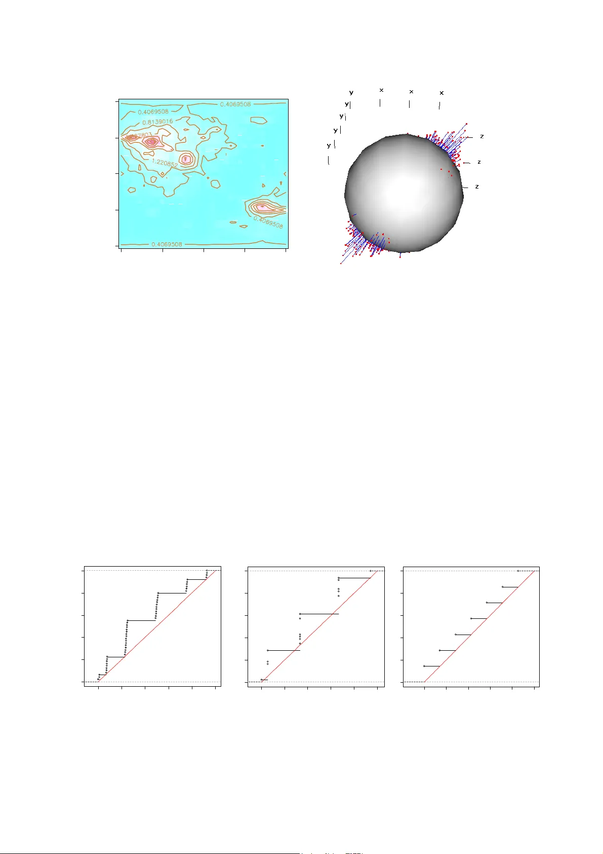
1 A R ADAR -S HAPED S TATISTIC FOR T ESTING AND V ISUALIZING U NIFORMITY P ROPER TIES IN C OMPUTER E XPERIMENTS Jessica Franco 1 , Laurent Carraro 1 , Olivier Roustant 1 and Astrid Jourdan 2 . 1 Département 3MI Ecole Nationale Supé rieure des Mines, Saint-Etienne, nom @emse.fr . 2 Ecole Internationale des Sciences du Tr aitement de l’Information, Pau, astrid.jourdan@eisti.fr . In the study of computer codes, filling sp ace as uniformly as possible is important to describ e the complexity of the investigate d phenom enon. Howeve r, this property i s not conse rved by reducing t he dim ension. Som e numeric expe riment design s are conceived in t his sense as Latin hy percubes or or thogonal arrays, b ut they consider only the projecti ons onto t he axes or the coordina te planes. In this article we introduce a statistic which allows study ing the g ood dist ribution of points acc ording to all 1-di mensional projectio ns. By a ngularly scan ning the domain, we obt ain a rada r type represen tation, allowi ng the unifo rmity defects o f a design to be i dentified with respect t o its pr ojections ont o straight lines. The advantage s of this new tool are dem onstrated on usual examples of space-filling designs (SFD) and a global statistic independent of the angle of rotation is studied. KEYWORDS: Computer experim ents ; Space-Filling De signs ; Dimension Reduction ; Discrepancy ; Kolmogorov-Smirnov Statistic, Cramer-Von Mises Statistic 1. INTRODUCTION For the last 15 years or so, the design of expe riment theory initiated by Fisher (1926) has experienced a revival for the anal ysis of costly industrial com puter codes. This development has led to at least two m ajor changes. First, these codes represent phenomena of an increas ing complexity, which implies that the corres ponding m odels are of ten nonlinear and/or nonparametric. Second, the experiment itself is different. Num erical experiments are simulations and, except for stochastic code s implem enting a Monte Carlo-based method, produce the same response for identical conditio ns (including algorithm and computer-based parameters). Therefore, repeating an experi ment under the sam e conditions does not make sense since no new information is acquired. In this new paradigm, the experiment plan ning m ethods are different. For example when the code is to be analyzed for the first time before any simulation has been made (scanning phase), one often tries to satisf y the following two requirements. Firstly, distribute the points in the space as uniformly as possible to catch n on-linearities; this exc ludes repetitions also. Secondly, this space coverage should remain well-distributed even when the effectiv e dimension is lowered. The first requirement was the starting point of re search work in space filling designs (SFD). The quality of the spatia l distribution is measured either by using deterministic criteria like minimax or m axi min distances (Johnson, Moore and Ylvisaker, 1990), or by using statistical criteria like discrepancy (Niederreite r, 1987, Hickernell, 1998, 2 Fang, Li, Sudjianto, 2006). The second requirement stems from the observation that codes often depend only on a few influential variables, which may be either direct factors or “principal components” composed of linear co mbinations of these variables. Therefore dealing only with these influential factors is more efficient. Note that dimension reducing techniques like SIR (Li, 1991) or KDR (Fukumizu, Bach, Jord an, 2004) effectively identify the space generated by the principal facto rs. He nce, it is desirable that the spa ce filling property should be also satisfied in the projection onto subspaces . This is the aim of Latin hypercubes designs (LHD) and orthogonal arrays (OA) in computer experiments. For instance, the space filling LHDs provide a un ifor m repartition in th e projection onto m argins, so that there is no loss of information if th e code depends on only one variable. In addition, orthogonal arrays with space-fillin g properties extend this aspect to higher dimensions (s ee, for example, Koehler and Owen, 1996, and m ore generally, Owen, 1992 or Santner, William s, Notz, 2003). Nevertheless, considering only the pr ojections onto margins is not sufficient if, for example, the code is a function of a linear combination of 2 variables. In this article we introduce a statistic ba sed on 1-dim ensional proj ections to test the uniformity for a design of experiment. The choice of 1 dimension is due to the difficulty in computing the theoretical distribution for hi gher dimensional space. The advantage of restricting to a single dimension is that it of fers a simp le viewing tool similar to a radar screen. By representing the statistic’s v alue in all directions, one obtains a parameterized curve (or surface), identif ying the uniformity defect s of a des ign with respect to its projections onto straight lines. The article is stru ctured as fo llows. In section 2 we define the new statistic and the associated visualization to ol, called un iformity radar, and give som e properties of them. In section 3 we show examples of radar applications to space-filling designs. Section 4 is devoted to extend the con cept by defining a global statistic which does not depend on a particular axis of rotation. In section 5, a di scussion on the uniformity radar allows specifying its scope of application. Proof s are given in the appendix. 2. UNIFORMITY RADAR In the analysis of a computer code, let us consider a uniform expe riment design on a cubic domain [] 1, 1 d Ω= − . Note 1 , ..., N x x the experimental points, and ( ) 0 H the hypothesis " 1 ,. . . , N x x were generated by independent random sampling according to the uniform distribution in Ω ". If the computer code depend s only on one principal component, the 3 projections on this axis should be we ll distributed. More generally, denote a L the straight line generated by the unitary vector ( ) 1 , ..., d aa a = of Ω , and a μ the probability distribution of the projections of 1 , ..., N x x onto a L . Ideally, we may expect that in any direction a the distribution a μ is uniform. However, this is not realistic when a L is not a coordinate axis. For example, in the case of the cubic dom ain [] 2 1, 1 − , the density of the projected design points is higher in the central part of the axis as can be seen in Figure 1. -1 .0 -0 .5 0.0 0.5 1 .0 -1.0 -0.5 0.0 0.5 1.0 -1 .0 -0 .5 0.0 0.5 1.0 0.0 0.2 0. 4 0.6 Figure 1. Left : Projecti ons of points ont o an axis L a . Right : The histogr am of the projections . More precisely, this distributi on is supported by 3 areas defi ned by the projection of the corners of the domain. The distribution a μ is continuous, with density represented below. The nodes of the trapezoidal density correspond to the corners of the square Ω projected onto the axis a L , where () cos , sin a θ θ = . Figure 2. The distribut ion of the projecti ons for a 3 dimens ional cubic domai n. In the general case, the projection onto a L is a linear combinati on of independent random variables of uniform distributi on, which lead s to a traditiona l problem of pr obabilities first 0 β α M -M - α where : M = |cos θ | + |sin θ | α = | |cos θ |-|sin θ | | β = α + M 1 4 solved by Lagrange in the 18th century (see discussion in Elias and Shiu (1987) on this topic). If we denote () 1 , ..., d X XX = , where 1 , ..., d X X are independent random variables identically distributed following the uni form distribution over [ ] 1, 1 − , and Z the projection of X onto a L , where 0 { 1 , ..., } j aj d ≠∀ ∈ , then the distribution function of Z is given by : F Z ( z ) = 1 2 a j j = 1 d ∏ ⎛ ⎝ ⎜ ⎜ ⎞ ⎠ ⎟ ⎟ × ε ( s ) ( z + s . a ) + d d ! s ∈ { − 1,1} d ∑ where () {} 1 , ..., 1 ,1 d d ss s =∈ − are the corners of the hypercube [] 1, 1 d Ω= − , 1 () d j j ss ε = = ∏ , . sa is the scalar product of the vectors s and a , and ( ) max ( , 0 ) y y + = the positive part of y . As a result, for a given axis, Z admits a piecewise linear density whose nodes correspond to the projections of the co rners of the domain. Note. The distribution of the projec tions is known in other situations, as in the ca se of a spherical domain: if Ω is the unit sphere of R d , a direct cal cul ation shows that a μ admits the density () [] () 2 1,1 2 11 a f xx x π − =− , the distribution function being equal to 2 11 () ( A r c s i n 1 ) 2 a Fx x x x π =+ + − for [ ] 1, 1 x ∈− . In sum, for a uniform experim ent design to have good distribution properties on the 1- dimensional projections, it will be n ecessary that in al l the dir ections a , the empirical distribution of the projections onto a L is close to their theore tical distribution under the hypothesis () 0 H . There exist many distribution ade quacy statistics (s ee D’agostino and Stephens, 1986), which allow for a large number of choices to define a criterion adapted for this purpose. How ever, possibilities are limited by special requirements. To start with, it is preferable that the statistic’s distribution be known to avoid the approximate calculation of its distribution. Furthermore, one would also like the statistic to be distribu tion free, that is, its distribution doesn’t depend on the projection direction to have a unique rejection threshold for all the angles. Also, for the sake of consistency, it would be desi rable for the retained statistic to be interpretable in term s of discrepancy wh en projections are m ade onto a coordinate axis. Finally, two famous statistics (at least) co rrespond to these requi rements: the Kolmogorov- Smirnov statistic 5 D N ( a ) = sup ˆ F N , a ( z ) − F a ( z ) (1) and the Cramér-Von Mises statis tic N ω N 2 ( a ) = ( ˆ F N , a ( z ) − F a ( z )) 2 dz ∫ (2) where , ˆ N a F is the empirical distribution function of the projections of 1 , ..., N x x onto a L , and a F the distribution function of a μ . When a L is a coordinate axis, a μ is the uniform distribution on [0,1] and these statistics co rrespo nd, respectively, to the discrepancies L ∞ and L 2 (Niederreiter, 1987). In what follows, we decided to work on the first because the conclusions seem equivalent, while the correspondi ng graph ics are a little more readable (see section 5). By analogy with the case of coordinate axes, we will talk about a discrepancy of projections to designate the Kolmogorov-Smirno v statistic of the formula (1). The discrepancy of projections p rovides a tool for visua lizing the defects in unif ormity based on the 1-dimensional projections. Since th is tool looks like a rad ar screen, we propose to call it uniformity radar . Its utilization depends on the dimension of Ω . In 2 dimensions, the discrepancy of projections is calculated in 360° by continuous ly projecting onto a rotating axis. Thus, one obtains a param eteri zed curve in polar coordinates ( ) N D θ θ a defined over [0,2 π ], called 2D radar . By displaying the quality of distributions in all directions, the 2D radar provid es decision support on design uniformity. In 3 dim ensions, one calculates the discrepancy of projections onto an axis , L θ ϕ , for all directions, pivoting around the center of the dom ain. This axis is defined in spherical coordinates by an angle θ in longitude and ϕ in latitude. This tim e a parameterized surface is obtained, called 3D radar , ( ) ( ) ,, N D θϕ θ ϕ a defined over [] 0, 2 , 22 π π π ⎡ ⎤ ×− ⎢ ⎥ ⎣ ⎦ . In higher dimensions, it seems unrealistic to make an angular scan of the space Ω . In addition, it becom es almost unfeasible to represent the result graphically (although the calculation is still possible). However, the hypothesis ( H 0 ) remains valid on 2- and 3-dimensional coordinate spaces. Therefore, the uniformity radar m ay be applied to all pairs and/or tr iplets of possible dimensions. In practice, the quality of the representation can be degraded by disc re tizing. Here the 2D and 3D radars are con tinuous applications. But N D is not differentiab le with respect to all the 6 axes a L so that at least two points of Ω are projected onto the sa me point, which explains why the parameterized curves of the next section are not smooth and contain m any singularities. 3. APPLICATIONS OF UNIFORMITY RADAR In this section we present a few examples to show the interest in us ing uniform ity radar to test the uniformity of the distribution of expe rimental points by looking at their projection. We consider cases where the hypothesis ( ) 0 H of a uniform distributi on in the experim ental domain is plausible. For each re pres entation of the uniformity radar we have added the circle (or the sphere) of radius ks equal to the statis tic of the Kolmogorov-Smirnov test associated with a 95% confidence level. Recall that since the s tatistic is distribution free, ks does not depend on a . This provides a decision-making support or, at least, a m eans of comparison with the random designs obtained by a unifor m sampling. Should the studied design be stochastic (pseudorandom, Latin hypercubes or randomized orthogonal arrays), the graph displays the directions a along which the hypothesis ( ) 0 H is rejected. If the design is deterministic, we are outside the usu al scope of a pplication of the test. If one of the values of () N Da is greater than ks , then we can only say that this de sign is worse than a random design since the probability that a random design will have a better discrepancy exceeds 95%. The following examples apply essentially to the la tter cases because we preferred to use known SFD designs without transforming them. Nonethel ess, in practice, it would suffice to apply randomization or scrambling (see, for exampl e, Fang, Li, Sudjianto, 2006) to obtain a stochastic design, and thus be under the usual assumptions of statistical tests. Example 1. Analysis of a 15-dimens ional Halton sequence using 2D radar. We consider the first 250 points of a 15-dimensional Halton sequence of low discrepancy (1960). Since the design is high dimensional, we apply the rada r to all pairs of possible dimensions. Among the rejected pairs we have, for example, the pair (14, 15), represented on Figure 3. 7 0.0 0.2 0 .4 0 .6 0.8 1.0 0.0 0.2 0.4 0 .6 0.8 1.0 -0.3 -0.2 -0 .1 0.0 0 .1 0.2 0.3 -0.3 -0 .2 -0.1 0.0 0 .1 0.2 0.3 Figure 3. Left: Design pr ojections of a Halto n sequence ont o the plane (X 14 ,X 15 ). Right: The 2D radar curve. In this example, since there exist values of ( ) N Da outside the circle of radius ks, the uniformity radar detects a non-uniform distribu tion for the 2-dimensional projections onto () 14 15 , XX . The largest deviation in uniformity is observed in direction a associated with an angle of approximately 135°, corresponding to the di rection that is perpen dicular to the visible diagonal alignments on the figure to the left. Here, we find ourselves faced with the well- known defect of high-dimensional Halton sequences, which do not preserve a low discrepancy in projection (Thi émard (2000), Morokoff, Caflisch (1994)). Note, however, that the radar is not designed to systematically detec t directions of alignm ent as we will see in the next example. Example 2. Analysis of orth ogonal arrays using 3D radar. Let us consider a 49 p oints linear orthogonal array of strength two in 3 dimensions (Owen (1992) and Jourdan (2000)). Like Latin hypercubes, these designs are of ten recommended for numeric experim ental designs because of their appreciable propertie s in pro jection. Projected onto a surface, an orthogonal array of strength two al ways yields a regular grid of points. However, the non- redundancy of the 2-dimensional projections does not imply a good distribution of the points neither on the axes of the domain (here 7 packets of 7 points) nor in th e 3D space, as we will see. X 15 X 14 Uniformity radar ks ≈ 0,09 8 Figure 4. Left. A 3-dimensi onal linear orthogonal a rray of strengt h two wit h 49 points. R ight. Projecti ons onto the plane ( X 1 ,X 2 ). The considered design is a linear orthogonal array of strength two. The way it is built implies that the points satisfy the relation x 1 +3x 2 +x 3 =0 (mod 7). Therefore, th ese points are located on 5 parallel planes. As a result, th e distribution of the projections onto the ax is perpendicular to these planes will not be satisf actory. This problem is never mentioned in computer experiments. However, it is well-known in the literature of experim ental designs. We applied the uniformity radar to the studied orthogonal array and represented the sphere of radius ks (the Kolmogorov-Smirnov sta tistic with a 95% confid ence level), the points () , N D θϕ , and drew straight lines join ing thes e points to the surface of the sphere to illustrate directionally the dev iations in uniform ity. We al so represented the loga rithm of the p-values of the Kolmogorov-Smirnov test as a function of θ and ϕ . We observe that the radar does indeed detect a problem in the dir ection perp endicular to the 5 planes, 72 , 18 θ ϕ =° = ° . In addition, it reveals a poor di stribution of the projected points onto the direction 35 , 40 θ ϕ =° = ° . This is a problem that we could not have anticipated from the design’s characteristics. 9 0.0 0.2 0.4 0.6 0.8 1.0 0.0 0.2 0.4 0.6 0.8 1.0 0.0 0.2 0.4 0 .6 0.8 1.0 0.0 0.2 0.4 0.6 0.8 1.0 0.0 0 .2 0.4 0 .6 0 .8 1.0 0.0 0.2 0.4 0.6 0.8 1.0 teta phi 0 45 90 135 180 -90 -45 0 45 90 Figure 5. Left. The p-values i n –log10 of t he Kolmogor ov-Smirnov test . Right. T he values of the Kolmogorov Smirnov test with the rada r’s representation in pins. However, the radar does not detect a problem on the coordinate axes, for which the projections are stacked in 7 packets of 7 poi nts. This can be explained by observing the empirical cumulative distribut ion function (ecdf). For exam ple, the deviation of the (transformed) ecdf of the pro jected points onto (Oz) from the unifo rm cdf is not large, as seen in Figure 6(c). Actually, the alignments can be detected by the Kolmogo rov-Smirnov statistic, especially when they are not regularly distributed in space (as in example 1). To illus trate this point, we represented the (trans formed) ecdf of the projected points onto the axis L1, L2, L3 corresponding to, respectivel y, the direction 35 , 40 θ ϕ = °= ° , the axis perpendicular to the 5 parallel planes, and (0z). The de viation in uniform ity is much larger on figures (a) and (b). Figure 6. Left to right. the distribution functions (after transformation) of the pro jected points onto L1, L2 and L3. (a) (b) (c) 10 4. A GLOBAL STATISTIC FOR 2D RADAR Example 3. Toward an extension of the uniformity radar. Let us consider the first 100 points of an 8-dimensional Halton sequen ce proj ected onto the subspace formed by () 36 , X X . 0.0 0.2 0.4 0.6 0.8 1.0 0 . 00 . 2 0 . 40 . 6 0 . 8 -0.1 5 -0.1 0 -0.0 5 0.0 0 0.05 0.1 0 0.1 5 -0.1 5 -0.1 0 -0.0 5 0 .0 0 0 .0 5 0 .1 0 0 .1 5 Figure 7. The f irst 100 ter ms of an 8 -dimensional Halton seque nce projec ted onto ( ) 36 , X X . Note that all the poin ts of the uniform ity radar are inside the circle of radius ks and, as a result, the radar accepts the design although we can see that the points of the plane () 36 , X X are not uniformly distributed. Howe ver, the discrepancy values are rather scattered with a low value for angle θ = 0°, and rather high values, for example, for angle 29 θ = ° , which seems to correspond to the orthogonal direction of alignments. The idea to reject this ty pe of design amounts, therefore, to defining a new sta tistic which introduces minimum and m aximum discrepancies. In order to avoi d scale problems, we suggest taki ng the ratio of these quantities. We have: [] [] 0,2 0,2 sup ( ) inf ( ) N N N D G D θπ θπ θ θ ∈ ∈ = (3) This statistic should filter out designs which have a relative poor distribution in one direction. This statistic has the advantag e of being global. This increas e the power of the corresponding statistical test. For a fixed va lue of N, the distribution of N G seems difficult to obtain other than by simulation. In the appendix, the tabl e corresponding to N=1…100 is given. According to this table, the rejection threshold at leve l 95% for a design of 100 poi nts is equal to 4.23. In 6 X 3 X 11 example 3, the observed value of the statistic N G is equal to 6.07, which very clearly eliminates this design. In the statistic table, we observe that the valu es stabilize as N increases, which leads us to believe that it is possib le to specify its asympt otic behavior. This is in fact the case. The following demonstration is based on th e theory of empirical processes. Asymptotic distribution of the global statis tic (3) . Let ( ) 1 , ..., N XX X = , where X 1 , ..., X N are independent random variable s from uniform distribution on [] 2 1, 1 − . Denote () R X θ as the projection of X on axis L θ . Let ( ) , t t N A A Y θ be the following process: ]] () ( ) () ( ) , , 11 11 1( ) ( ) 1 t t NN N iA i t t A ii YR X P R X t X P X A NN θ θθ −∞ == =− < = − ∈ ∑∑ where A t = x ∈ R d , R θ ( x ) < t { } . Using these notations, the discrepancy of projecti ons may be written as () , sup t N N A t DY θ θ ∈ =  . Therefore, , , sup ( ) sup sup inf ( ) inf sup t t N N A t N N N A t DY G D Y θ θθ θ θ θ θ θ == . The limit distribution of the process ( ) , t t N A A Y θ is obtained using the theory of empirical processes. With the central limit theorem , one obtains the convergence of the finite dimensional distributions toward the Gaussian process of sam e expectation and covariances. Furthermore, the fam ily ( A t ) t is a VC-class (see …). Therefore, ( ) ( ) , tt tt loi N AA A A YY θθ ⎯⎯ → where ( ) t t A A Y θ is a centered Gaussian process with covariance: 12 ( ) () () () () () () () ( ) () ( ) () ( ) 2 , 1 cov , ( ) , ( ) 1 () . () 1 () . () () . () cov , ( ) , ( ) ( ) . ( ) cov , ( ) ( ). ( ). st st st N AA ij N i N j AA st s t AA YY P R X s R X t N PR X s PR X t N PR X t PR X s N PR X s PR X t YY P R X s R X t P R X s P R X t YY P A A P A P A μ θ μθ μθ θμ μθ μ θ μθ μ θ μ θ =< < −< < −< < +< < = << − < < =∩ − ∑ ∑ ∑ (4) and P ( G N < y ) N →+∞ ⎯ → ⎯ ⎯ P sup θ sup t Y A t θ inf θ sup t Y A t θ < y ⎛ ⎝ ⎜ ⎜ ⎞ ⎠ ⎟ ⎟ The probability ( ) s t PA A ∩ is interpreted as th e surface of a polygon delimited by the domain and the straight lines s t Ae t A (see Figure 8) . This su rface can be analytically calculated, by noting (for example) that the polygon is a parti tion of triang les with a common corner to be selected from among the vertices of the polygon. The asymptot ic distribution of N G can then be obtained by simulating a centere d Gaussian field with covarian ce matrix defined by (4). Figure 8. Interpretation of the probability () PA A s t ∩ . The procedure is semi-analytic because sim ulati ons are need ed to perform the calculations. In theory, the global statistic may be e xtended to 3 dimensions. For a f inite sample, the sta tistic 1 O=(0,0) L μ t s t A s A -1 1 -1 L θ 13 table can be calculated with sim ulations. Howeve r, the asymptotic distribution is much more difficult to obtain. 5. DISCUSSION Due to the complexity of the phenomena simulated by com puter codes, which implies non- linearities, distributing numerical experiments as uniform ly as possible in the dom ain is preferable. In addition, this distribution shoul d continue to be satisfactory when projecting onto subspaces, especially when the code de pends only on a small number of factors or principal components. In this article we introduce a statistic based on 1-dim ensional projections to test the uniform ity for a design of experiment . In 2 and 3 dimensions, it provides a simple viewing tool called uniformity radar, which graphically tests the uniformity hypothesis by omni-directional scanning. Moreove r, we introduced a global statistic in 2 dimensions to further identify unsatisfactory designs that had been accepted by the uniform ity radar. These tools were applied on usual SFD designs. On these case studies, some of the designs have very poor properties when projecting to su bspaces, as the 15-dimensional sequence with low discrepancy in example 1 or the 3-dimensional orthogonal array in example 2. The uniformity radar was able to detect these defect s. It succeeds when there is a rectangular shaped empty area in the domain, as in th e aforementioned examples. In such cases, th e distribution is unsatisfactory wh en projecting onto the rectangle’ s width. The uniformity radar can also detect the alignments of points, but m ay not identify them if the directions of alignments are well distributed su ch as with a factorial design (see example 2). This underscores the lack of power of the Kolmogorov-Smirnov test when the sample is generated from a continuous distribution supported by the union of small intervals regularly distributed. In practice, this situation is not very detrimental because th e SFD obtained by a deterministic process are often randomized or scrambled (see, for exam ple, Fang, Li and Sudjianto, 2006). Our uniformity radar may be adapted to othe r goodness-of-fit statistics, such as Cramér- Von Mises (see section 2), which corresponds to the discrepancy L 2 for a projection onto a coordinate axis. For instance, we repeated the examples 1 to 3 with the corresponding radar. As expected, the conclusions are the sam e because the Kolmogorov-Smirnov and Cram ér- Von Mises tests do not present a ny clear-cut difference in term s of power. Interestingly, the main difference is graphic. The curve of th e radar defined with the Cramér-Von Mises statistic is smoother, which is due to the no rm L 2 , and introduces sometim es large scale 14 variations from one design to another, while these differences are attenuated by the norm L ∞ in the examples given here . For this reason, the L ∞ radar may be preferred because the conclusions are more apparent. Figure 9. Uniformity radar with the Cramér-Von Mises statistic for examples 1 and 3 . ACKNOWLEDGMENTS This work was conducted within the frame of th e DICE (Deep Inside Computer Experiments) Consortium between ARMINES, Renault, EDF, IRSN, ONERA and TOTAL S.A. We also thank Chris Yukna for his help on editing. 15 APPENDICES Distribution of a linear combination for uni formly distributed independent variables. The final result demonstrated by Ostrowski (1952) often uses very technical methods. However, Elias et al. (1987) propose a simp ler operational computational m ethod that we apply to our special case. Let 11 . ... dd Z Xa X a X a == + + . This is, therefore, a sum of independent random variables of uniform distribution on [ ] , , 1 , ..., ii aa i d −= . As a result, it admits the density given by [] [] () 11 ,, 1 1 11 2 dd d Z aa a a j j f a −− = ⎛⎞ =× ∗ ∗ ⎜⎟ ⎜⎟ ⎝⎠ ∏ L , where ∗ designates the convol ution product. To calculate this product of convolut ions, Elias et Shiu (1987) s uggest using translations. Let () () ( ) a Tfx f x a =+ , the translation of the function f from - a. Then we can write (with the convention 0 0 , 0 α α =∀ ≥ ): ( ) ( ) () () () () 00 , 00 0 1( ) () () () jj jj jj jj aa aa aa xx a x a Tx x T x x TT x x ⎡⎤ − ++ ⎣⎦ +− + −+ =+ − − =− =− And, therefore, () () () () ( ) 11 00 1 1 () 2 dd d Za a a a j j f xT T x T T x a − +− + = ⎛⎞ =× − ∗ ∗ − ⎜⎟ ⎜⎟ ⎝⎠ ∏ L . The proof follows from two basic lemmas. Lemma 1. The translation comm utes with the convolution. () ( )( ) 12 1 2 1 2 12 () ( ) , ax x x ax a x x Tf f f Tf T f f x x ∗= ∗ = ∗ ∀ ∈  Lemma 2. () 1 ,, !! 1 ! mn m n xx x nm x mn m n ++ ++ + ∗= ∀ ∈ ∀ ∈ ++  By applying lemma 1, we obtain: () () () () 11 00 1 1 () 2 dd d Za a a a j j df o i s fx T T T T x x a −− + + = ⎛⎞ ⎛⎞ ⎜⎟ =× − − ∗ ∗ ⎜⎟ ⎜⎟ ⎜⎟ ⎜⎟ ⎝⎠ ⎝⎠ ∏ LL 1 4 42 4 4 3 . 16 Then by applying lemma 2: () ( ) () 11 2 2 1 1 1 ( ) ... 2( 1 ) ! dd d d Za a a a a a j j x fx T T T T T T ad − + −− − = ⎛⎞ ⎛⎞ =× − − − ⎜⎟ ⎜⎟ ⎜⎟ ⎜⎟ − ⎝⎠ ⎝⎠ ∏ . and {} () 11 1 1 1 1,1 1 () 2( 1 ) ! dd d d d Zd s a s a j j s x fx s s T T ad − + = ∈− ⎛⎞ ⎛⎞ ⎜⎟ =× ⎜⎟ ⎜⎟ ⎜⎟ − ⎝⎠ ⎝⎠ ∑ ∏ LL . Finally, 1 1 (. ) 1 () ( ) 2( 1 ) ! d d Z j s j xs a fx s ad ε − + = ⎛⎞ ⎛⎞ + =× ⎜⎟ ⎜⎟ ⎜⎟ ⎜⎟ − ⎝⎠ ⎝⎠ ∑ ∏ . The announced result is obtained by integrating this relation  Continuity and differentiability of the radar. For the sake of simplicity, we give only the pr oofs in 2 dimensions. However, the result is also valid in 3 dimensions. Let () () 1 1 ,..., [0 , 1 ] ˆ ,, s u p N U Nz z z Dz z F zz ∈ = − K , the Kolmogorov- Smirnov statistic for the uniform distribution over [ ] 0, 1 . Proposition. (i) U D is continuous. (ii) U D admits partial deriv atives w ith respect to all the , 1 , ..., i x iN = in () 1 , ..., N zz if and only if the supremum of () 1 ,... , ˆ N zz Fz z − is attained at only one { } , 1 , ..., j zj N ∈ . Proof . Let () ( ) () () 11 cos sin , , cos sin U NN N DD F x y F x y θθ θ θθ θ θ =+ + K where () () 1 1 ,..., [0 , 1 ] ˆ ,, s u p N U Nz z z Dz z F zz ∈ = − K is the Kolmogorov-Smirnov statistic for the uniform distribution over [ ] 0, 1 . By using the expression of F θ , we prove that () ( ) , p Fp θ θ a is continuous ( cf. formula (2.1)). Thus, the problem reduces to demonstrate the continuity of () {} 1 1 1 , ..., sup 1 i N N tt t i tt t N > = − ∑ a with respect to all variables. If the values of i t are perturbed by i η , the supremum varies at most by the sum of the i η , thereby guaranteeing continuity. 17 For differentiability, the problem can be reduced to the existence of partial derivatives of U D . • Let us assume that the suprem um is attained f or only one j z where { } 1 , ..., j N ∈ . In this case, the partial derivatives r elated to i z , ij ≠ , exist and are equal to 0 because any local perturbation in i z would not change the supremum. Let us now prove the existence of U j D z ∂ ∂ . Let us assume, for example, that: [0 , 1 ] ˆˆ sup ( ) ( ) 0 NN j j z Fz z Fz z ∈ − =− > . We choose ε such that ˆˆ ,( ) ( ) Nj j N i i ij F z z F z z ε ∀≠ − > − + et ˆ () Nj j Fz z ε − > . Then : () ( ) 11 , ..., , ..., , ..., UU jN j Dz z z Dz z ε ε += − et ( )( ) 11 , ..., , ..., , ..., UU jN j Dz z z Dz z ε ε − =+ Therefore, () 1 , ..., U N j D zz z ∂ ∂ exists in ( ) 1 , ..., N zz and is equal to -1. Similarly, if ( ) [0 , 1 ] ˆˆ sup ( ) Nj N j z Fz z z F z ∈ −= − , we prove that U j D z ∂ ∂ exists and is equal to 1.  Let us assume that the suprem um is attained at j z and at least at another k z for { } , 1 , ..., j kN ∈ . Now, we are going to prove that the partial derivative in j z does not exist. Assume, for example, that ˆ () 0 Nj j Fz z − > and 0 ε > , ˆ () Nj j Fz z ε − > . Then we have the following case.  The supremum is at j z and k z , jk ≠ where jk zz = . Then () () 11 , ..., , ..., , ..., UU jN N Dz z z Dz z ε ε + =− , but () () 11 , ..., , ..., , ..., UU jN N Dz z z Dz z ε −= . Therefore, the right -hand derivative is different from the left-hand derivative. • Otherwise, for all k z , where kj ≠ at w hich the supremum is atta ined, jk zz ≠ . Thus () () 11 , ..., , ..., , ..., UU jN N Dz z z Dz z ε ε − =+ but () () 11 , ..., , ..., , ..., UU jN N Dz z z Dz z ε += because the local perturbation in j z does not change the value of the suprem um, wh ich is still attained at k z . , the righ t-hand derivative is therefore also differe nt from the left-hand derivative.  18 Table of the statistic of N G : values of N g such that () N N PP G g = < . N P=0,80 P=0,85 P=0,90 P=0,95 P=0,99 1 1,94 1,97 1,98 1,99 1,99 2 2,52 2,82 3,08 3,33 3,47 3 2,68 3,00 3,30 3,63 3,84 4 2,80 3,12 3,42 3,80 4,07 5 2,86 3,19 3,50 3,88 4,12 6 2,89 3,25 3,58 3,97 4,26 7 2,93 3,28 3,59 4,01 4,28 8 2,94 3,29 3,64 4,03 4,31 9 2,95 3,30 3,61 4,00 4,35 10 2,97 3,34 3,66 4,06 4,33 11 2,98 3,34 3,68 4,13 4,46 12 2,99 3,33 3,67 4,08 4,34 13 3,00 3,36 3,70 4,11 4,40 14 3,00 3,36 3,72 4,11 4,41 15 3,00 3,34 3,68 4,12 4,43 16 3,00 3,36 3,70 4,10 4,43 17 3,03 3,38 3,70 4,13 4,49 18 3,01 3,35 3,68 4,07 4,39 19 3,04 3,41 3,75 4,15 4,50 20 3,04 3,41 3,74 4,15 4,47 21 3,04 3,40 3,73 4,17 4,48 22 3,05 3,41 3,74 4,12 4,42 23 3,05 3,39 3,73 4,16 4,47 24 3,06 3,42 3,73 4,16 4,42 25 3,05 3,40 3,72 4,15 4,48 26 3,06 3,43 3,74 4,11 4,46 27 3,05 3,40 3,72 4,11 4,44 28 3,06 3,41 3,76 4,18 4,49 29 3,06 3,43 3,75 4,17 4,47 30 3,05 3,42 3,76 4,18 4,49 31 3,06 3,40 3,72 4,11 4,41 32 3,07 3,44 3,79 4,27 4,58 33 3,06 3,40 3,71 4,12 4,43 34 3,05 3,40 3,71 4,13 4,41 35 3,07 3,42 3,76 4,17 4,42 36 3,08 3,43 3,76 4,16 4,47 37 3,09 3,46 3,78 4,21 4,53 38 3,08 3,45 3,78 4,16 4,47 39 3,07 3,44 3,77 4,23 4,53 40 3,06 3,42 3,75 4,17 4,45 41 3,08 3,43 3,76 4,16 4,53 19 42 3,09 3,43 3,76 4,18 4,47 43 3,08 3,44 3,75 4,21 4,53 44 3,10 3,45 3,76 4,15 4,51 45 3,09 3,44 3,77 4,17 4,44 46 3,07 3,43 3,75 4,15 4,52 47 3,07 3,43 3,78 4,22 4,51 48 3,07 3,42 3,75 4,15 4,41 49 3,10 3,44 3,78 4,21 4,50 50 3,08 3,44 3,77 4,21 4,53 51 3,09 3,43 3,77 4,18 4,47 52 3,11 3,45 3,79 4,22 4,54 53 3,09 3,46 3,78 4,15 4,48 54 3,10 3,45 3,81 4,24 4,54 55 3,09 3,44 3,76 4,20 4,50 56 3,10 3,44 3,79 4,19 4,52 57 3,09 3,46 3,79 4,19 4,48 58 3,09 3,45 3,78 4,20 4,49 59 3,11 3,44 3,78 4,18 4,52 60 3,08 3,44 3,76 4,17 4,45 61 3,11 3,47 3,82 4,20 4,54 62 3,10 3,47 3,80 4,19 4,48 63 3,09 3,45 3,78 4,19 4,46 64 3,09 3,47 3,79 4,23 4,53 65 3,10 3,47 3,80 4,22 4,54 66 3,11 3,46 3,78 4,16 4,45 67 3,10 3,45 3,79 4,23 4,52 68 3,09 3,43 3,77 4,15 4,44 69 3,09 3,44 3,77 4,18 4,44 70 3,10 3,46 3,78 4,21 4,50 71 3,11 3,46 3,77 4,17 4,49 72 3,10 3,44 3,78 4,18 4,42 73 3,09 3,45 3,79 4,18 4,54 74 3,11 3,47 3,80 4,17 4,46 75 3,10 3,44 3,77 4,21 4,47 76 3,11 3,48 3,80 4,22 4,51 77 3,09 3,43 3,78 4,19 4,44 78 3,11 3,45 3,78 4,21 4,48 79 3,08 3,44 3,78 4,20 4,46 80 3,10 3,46 3,80 4,21 4,52 81 3,11 3,48 3,79 4,19 4,52 82 3,11 3,49 3,83 4,25 4,51 83 3,11 3,46 3,78 4,17 4,44 84 3,11 3,45 3,77 4,18 4,51 85 3,09 3,46 3,77 4,23 4,55 20 86 3,10 3,46 3,78 4,18 4,49 87 3,08 3,44 3,76 4,15 4,44 88 3,11 3,47 3,77 4,21 4,48 89 3,10 3,47 3,79 4,17 4,46 90 3,08 3,43 3,74 4,15 4,44 91 3,07 3,43 3,76 4,14 4,43 92 3,09 3,46 3,78 4,19 4,52 93 3,09 3,46 3,81 4,23 4,53 94 3,08 3,43 3,74 4,18 4,52 95 3,09 3,44 3,77 4,21 4,54 96 3,11 3,45 3,76 4,19 4,52 97 3,12 3,45 3,78 4,20 4,47 98 3,08 3,44 3,79 4,21 4,46 99 3,09 3,45 3,77 4,21 4,50 100 3,10 3,44 3,79 4,23 4,51 21 REFERENCES D’agostino R.B., Stephens M.A. (1986). Goodness-of-fit Techniques . Marcel Dekker, New- York. Elias S.W., Shiu W . (1987). Convolution of Uniform Distributions and Ruin Probability. Scandinavian Actuarial , 191-197. Fang K.-T., Li R., Sudjianto A. (2006). Design and Modeling for Computer Experiments . Chapman & Hall. Fisher, R.A. (1926). The arrang ement of field experim ents. J. Ministry Agric . 33 , 503-513. Fukumizu K., Bach F.R., Jordan M.I. (2004), Dimension Reduction for Supervised Learning with Reproducing Kernel Hilbert Spaces, Journal of Machine Learning Research , 5 , 73- 99. Halton, J.H. (1960). On the efficiency of cer tain quasi-random sequences of points in evaluating multi-dim ensional integrals, Numer. Math, 2 , 84-90. Hickernell, F. (1998). A generalized di screpancy and quadrature error bound, Mathematics of computation , 67 , 299-322. Koehler, J.R. et Owen, A.B. (1996). Computer Experim ents, Handbook of Statistics , 13 , 261- 308. Jourdan A. (2000). Analyse statistique et échantillonnage d’expériences simulées, Université de Pau et des Pays de l’Adour. Li K-C. (1991). Sliced i nverse regression for dimension reduction (with discussion). Journal of the American Statistical Association , 86 , 316-342. Morokoff, W.J., Caflisch R.E. (1994). Quasi -random sequences and their discrepancies. S.I.A.M. Journal Scientific Computing, 15 , 1251-1279. Niederreiter, H. (1987). Low-Discrepancy and Low-Dispersion Sequences, Journal of number theory, 30 , 51-70. Ostrowski A.M. (1952). Two Explicit Formulae fo r the Distribution Function of the Sum s of n Uniformly Distributed Independent Variables, Arch. Math , 3 , 451-459. Owen A.B. (1992). Orthogonal arrays for co mputer experiments, integration and visualization. Statisitica Sinica 2 , 439-452. Santner T.J., William s B.J., Notz W.I. (2003). The Design and Analysis of Computer Experiments , Springer. Thiémard E. (2000). Sur le calcul et la majora tion de la discrépance à l'origine. Thèse No 2259, Département de mathématiques, école polytechnique fédérale de Lausanne.