Combining Expert Advice Efficiently

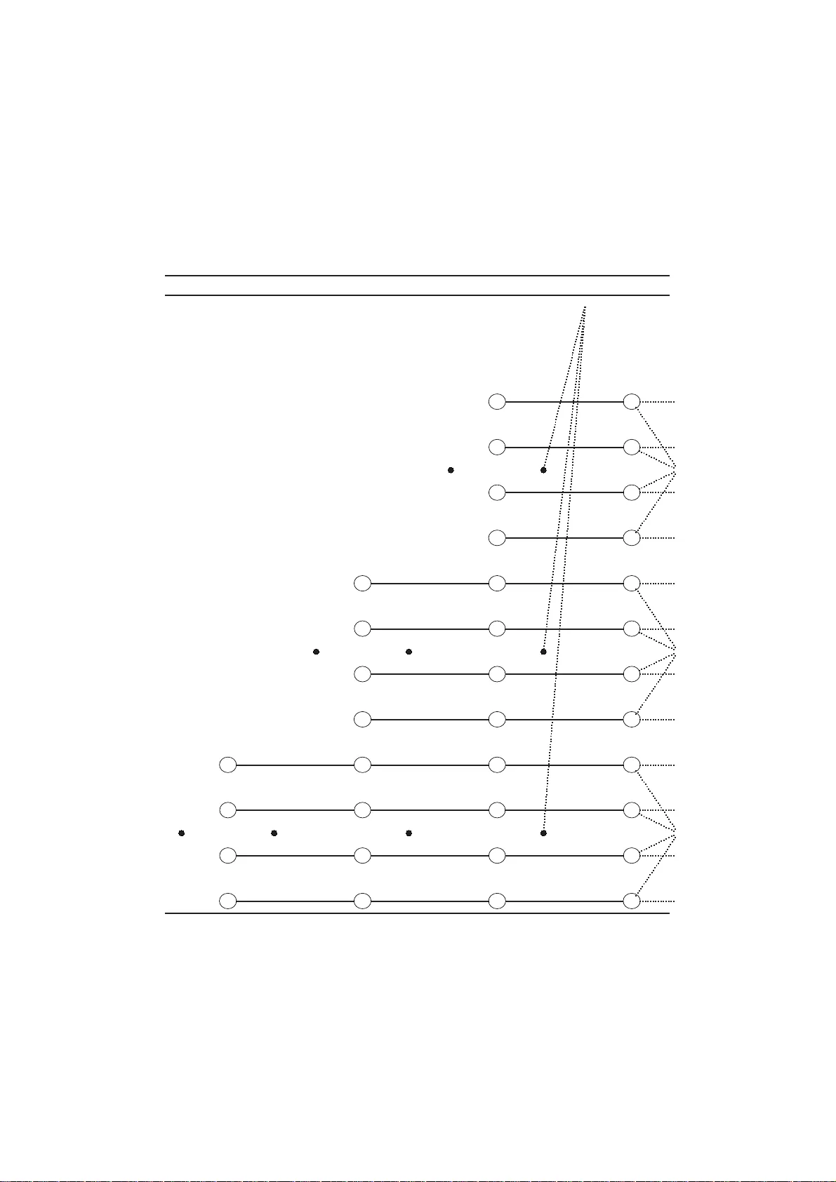
Combining Exper t Advice Efficientl y W outer Ko olen Stev en de R oo ij Cen trum v o or Wiskunde en Informatica (CWI) Kruislaan 413, P .O. Bo x 94079 1090 GB Amsterdam, The Netherlands { W.M.Koo len-Wijkstra,S.de.Rooij } @cwi.nl Con ten ts 1 In tro duction 1 2 Exp ert Sequence Priors 4 2.1 Examples . . . . . . . . . . . . . . . . . . . . . . . . . . . . . 6 3 Exp ert T racking using HMMs 7 3.1 Hidden Mark o v Mod els Ov erview . . . . . . . . . . . . . . . . 7 3.1.1 Algorithms . . . . . . . . . . . . . . . . . . . . . . . . 9 3.2 HMMs as ES-Priors . . . . . . . . . . . . . . . . . . . . . . . 10 3.3 Examples . . . . . . . . . . . . . . . . . . . . . . . . . . . . . 12 3.4 The HMM f or Data . . . . . . . . . . . . . . . . . . . . . . . 13 3.5 The F orward Algorithm and Sequent ial Prediction . . . . . . 14 4 Zo ology 18 4.1 Univ ersal Elemen twise Mixtures . . . . . . . . . . . . . . . . . 19 4.1.1 A Loss Boun d . . . . . . . . . . . . . . . . . . . . . . . 19 4.1.2 HMM . . . . . . . . . . . . . . . . . . . . . . . . . . . 20 4.2 Fixed Sh are . . . . . . . . . . . . . . . . . . . . . . . . . . . . 21 4.3 Univ ersal Share . . . . . . . . . . . . . . . . . . . . . . . . . . 23 4.4 Ov erconﬁdent Exp erts . . . . . . . . . . . . . . . . . . . . . . 25 4.4.1 Recursiv e Com bination . . . . . . . . . . . . . . . . . 26 5 New Mo de ls to Switc h b et ween Exp erts 27 5.1 Switc h Distribution . . . . . . . . . . . . . . . . . . . . . . . . 28 5.1.1 Switc h HMM . . . . . . . . . . . . . . . . . . . . . . . 29 5.1.2 Switc h Distribution . . . . . . . . . . . . . . . . . . . 29 5.1.3 Equiv alence . . . . . . . . . . . . . . . . . . . . . . . . 31 5.1.4 A Loss Boun d . . . . . . . . . . . . . . . . . . . . . . . 32 5.1.5 MAP Estimation . . . . . . . . . . . . . . . . . . . . . 34 5.2 Run-length Mo del . . . . . . . . . . . . . . . . . . . . . . . . 36 5.2.1 Run-length HMM . . . . . . . . . . . . . . . . . . . . 37 5.2.2 A Loss Boun d . . . . . . . . . . . . . . . . . . . . . . . 37 5.2.3 Finite S upp ort . . . . . . . . . . . . . . . . . . . . . . 40 6 Extensions 40 6.1 F ast Ap pro ximations . . . . . . . . . . . . . . . . . . . . . . . 40 6.1.1 Discretisatio n . . . . . . . . . . . . . . . . . . . . . . . 41 6.1.2 T rimming . . . . . . . . . . . . . . . . . . . . . . . . . 41 6.1.3 The ML Conditioning T rick . . . . . . . . . . . . . . . 41 6.2 Data-D ep endent Priors . . . . . . . . . . . . . . . . . . . . . . 44 6.3 An Alternativ e to MAP Data Analysis . . . . . . . . . . . . . 44 7 Conclusion 45 1 Abstract W e sh o w ho w mo dels for prediction with exp ert advice can b e d eﬁned con- cisely and c learly using hidden Mark o v mo dels (HMMs); standard HMM al- gorithms can then b e used to eﬃcien tly calculate, among other things, how the exp ert predictions sh ould b e w eigh ted according to the mo del. W e cast man y existing mo dels as HMMs and reco v er the b est k n o wn r unning times in eac h case. W e also describ e tw o new m odels: the switc h distribution, whic h w as r ecently deve lop ed to impro v e Ba y esian/Minim um Description Length mo del selection, an d a n ew generalisation o f the ﬁxed share algorithm based on run-length co ding. W e giv e lo ss boun ds f or all mo dels and shed new ligh t on their relationships. 1 In tro duction W e cannot predict exactly ho w complicated pr o cesses suc h as the wea ther, the stoc k marke t, so cial in teractions and so on, will dev elop in to the fu ture. Nev ertheless, p eople do ma ke we ather forecasts and buy shares all the time. Suc h predictions can b e based on formal mo dels, or on human exp ertise or int uition. An inv estmen t compan y m a y ev en wa nt to c ho ose b et wee n p ortfolios on the basis of a co mbination of these kinds of pr edicto rs . In s u c h scenarios, predictors typica lly cann ot b e considered “true”. Thus, we ma y w ell end up in a p osition where w e ha ve a wh ole collect ion of pr edictio n strategies, or exp erts , eac h of whom has some in sigh t into some asp ects of the pr ocess of in terest. W e add r ess the qu estion ho w a giv en set of exp erts can b e com bined into a single pr edictiv e strategy th at is as go od as, or if p ossible ev en b etter than, the b est in dividual exp ert. The setup is as follo ws. Let Ξ b e a ﬁnite set of exp erts. Eac h exp ert ξ ∈ Ξ issues a d istribution P ξ ( x n +1 | x n ) on the next outcome x n +1 giv en th e previous observ ations x n := x 1 , . . . , x n . Here, eac h outcome x i is an elemen t of some coun table space X , and random v ariables are written in b old face. The probabilit y that an exp ert assigns to a sequence of outcomes is given b y th e c hain rule: P ξ ( x n ) = P ξ ( x 1 ) · P ξ ( x 2 | x 1 ) · . . . · P ξ ( x n | x n − 1 ). A standard Ba yesia n app roac h to com bine the exp ert predictions is to deﬁne a prior w on the exp erts Ξ whic h indu ces a join t distribu tion with mass function P ( x n , ξ ) = w ( ξ ) P ξ ( x n ). Inference is then b ased on this joint distribution. W e can compute, for example: (a) the mar g inal pr ob ability of the data P ( x n ) = P ξ ∈ Ξ w ( ξ ) P ξ ( x n ), (b) th e pr e d ictive distribution on the next outco me P ( x n +1 | x n ) = P ( x n , x n +1 ) /P ( x n ), whic h deﬁnes a predictio n strategy that com bines th ose of the individual exp erts, or (c) the p osterior distribution on the exp erts P ( ξ | x n ) = P ξ ( x n ) w ( ξ ) /P ( x n ), which tells u s ho w th e exp erts’ pr edictio ns should b e w eigh ted. This simp le p robabilistic approac h has the adv ant age that it is computationally easy: predicting n outcomes u s ing | Ξ | exp erts requ ires only O ( n · | Ξ | ) time. Additionally , this Ba y esian strategy g u arantees th at the o v erall pr obabilit y of the data is only a facto r w ( ˆ ξ ) smaller than the probability of th e dat a according to the b est a v ailable exp ert ˆ ξ . On the ﬂip side, with this strategy we n ev er do any b etter than ˆ ξ either: w e ha v e P ˆ ξ ( x n ) ≥ P ( x n ) ≥ P ˆ ξ ( x n ) w ( ˆ ξ ), which means that p oten tially v aluable in sigh ts from the other exp erts are not used to our adv ant age! More sophisticated com binations of p rediction strategies can b e found in the literature u n der v arious headings, including (Ba ye sian) statistics, sou r ce co ding and universal p rediction. I n the latter the exp erts’ pr edictio ns are not necessarily p robabilistic, and scored us ing an arb itrary loss fun ction. In th is pap er we consider only logarithmic loss, although our resu lts can undoub tedly be generalised to the framework describ ed in, e.g. [14]. W e int ro duce HMMs as an int uitive graphical language that allo ws uni- 1 ﬁed description of existing and new mo dels. Additionally , the run ning t ime for ev aluation of su c h mo dels can b e read oﬀ d irectl y fr om the size of their represent ation. Ov erview In Section 2 w e dev elop a more general framew ork for com bining exp ert predictions, where we consider th e p ossibilit y t hat the optimal we ights used to mix the exp ert predictions may v ary over time , i.e. as th e sample size increases. W e stic k to Ba y esian metho dology , but w e d eﬁne the prior dis- tribution as a p robabilit y measure on se quenc es of exp erts r ather than on exp erts. The prior probabilit y o f a sequence ξ 1 , ξ 2 , . . . is the p robabilit y t h at w e rely on exp ert ξ 1 ’s prediction of the ﬁrs t outcome and exp ert ξ 2 ’s pre- diction of the second outcome, etc. This allo ws for the expr ession of more sophisticated mo dels for the com bin atio n of exp ert predictions. F or example, the natur e of the data generating p rocess ma y ev olv e o v er time; consequ ently diﬀeren t exp erts ma y b e b etter during diﬀeren t p erio ds of time. I t is also p ossible that not the d ata generating pro cess, bu t the exp erts themselv es c hange as more and more outcomes are b eing obs er ved: th ey ma y learn from past mistak es, p ossibly at diﬀerent r ate s, or they may ha ve o cca sional bad da ys, etc. In b oth situations we ma y hop e to b eneﬁt f rom more sophisticated mo delling. Of course, n ot all m odels for com bin ing exp ert predictions are compu- tationally f easible. S ecti on 3 describ es a metho dology for the s p eciﬁcatio n of mo dels that allo w eﬃcient ev aluation. W e ac hieve this b y using hidden Mark o v mo dels (HMMs) on t wo lev els. On the ﬁrst lev el, we use an HMM as a formal sp eciﬁcation of a distribu tion on sequences of exp erts as deﬁned in Section 2. W e introd uce a graphical language to con venien tly represent its structure. Th ese graphs help to u nderstand and compare existing m od- els and to design n ew ones. W e then mo dify this ﬁrst HMM to construct a second HMM that sp eciﬁes the distribution on sequences of outc omes . S ub- sequen tly , w e can us e the standard dynamic programming algorithms for HMMs (forward, bac kw ard and Viterbi) on b oth lev els to eﬃcien tly calcu- late most relev an t quantit ies, most im p ortan tly the marginal probabilit y of the observed outcomes P ( x n ) and p osterior w eigh ts on the next exp ert giv en the previous obser v ations P ( ξ n +1 | x n ). It turns out that m an y existing mo dels for pr edictio n with exp ert advice can b e sp eciﬁed as HMMs. W e pro vide an o verview in S ecti on 4 by giving the graphical represent ations of the HMMs corresp onding to the f ollo wing mo dels. First, univ ersal elemen t wise mixtur es (sometimes called mixture mo dels) that learn the optimal mixtur e parameter from data. S econd, He rb - ster and W armuth’s ﬁxed share algorithm fo r tracki n g the b est exp ert [5 , 6]. Third, u niv ersal share, whic h was introdu ced by V olf and Willems as th e “switc hing metho d” [13] and later indep enden tly prop osed by Bousquet [1]. 2 Figure 1 Ex p ert sequence p riors: generalisation relationships and run time ﬁxed exp ert v v l l l l l l l l l l l l l l l l l " " D D D D D D D D D O ( n ) _ _ _ _ _ _ _ _ _ _ _ _ _ _ _ _ _ _ _ _ _ _ _ _ _ _ _ _ _ _ _ _ _ _ _ _ _ _ ﬁxed elemen twise mixture ) ) S S S S S S S S S S S S S S S S S   Ba yesian mixture { { w w w w w w w w % % J J J J J J J ﬁxed share $ $ J J J J J J J                    ﬁxed o verconﬁdent exp erts   O ( n | Ξ | ) switc h distribution _ _ _ _ _ _ _ _ _ _ _ _ _ _ _ _ _ _ _ _ _ _ _ _ _ _ _ _ _ _ _ _ _ _ _ _ _ _ run-length mod el universal share universal o verconﬁdent exp erts O ( n 2 | Ξ | ) _ _ _ _ _ _ _ _ _ _ _ _ _ _ _ _ _ _ _ _ _ _ _ _ _ _ _ _ _ _ _ _ _ _ _ _ _ _ universal elemen twise mixture O ( n | Ξ | ) Here the goal is to learn the optimal ﬁxed-sh are parameter from d ata. Th e last considered mo del safeguards against ov erconﬁd en t exp erts, a case ﬁrst considered b y V o vk in [14]. W e rend er eac h model as a prior on s equ ences of exp erts b y giving its HMM. The size of the HMM immediately determines the required running time for the fo rward al gorithm. T he generalisation re- lationships b et we en these mo dels as w ell as th eir runnin g times are displa yed in Figure 1. In eac h case this ru nning time coincides with that of the b est kno wn algorithm. W e also giv e a loss b ound for eac h mo del, relating the loss of the mo del to the loss of the b est comp etitor among a set of alternativ es in the wo rst c ase. Such loss b ound s can help select b etw een diﬀeren t mo dels for sp eciﬁc prediction tasks. Besides the mo dels found in the literature, Figure 1 also includes t wo new generalisations of ﬁxed share: the s w itc h distribu tion a nd the ru n-length mo del. Th ese mo dels are the sub ject of Section 5. The switc h distrib ution w as introd u ced in [12] as a practical means of improving Ba ye s/Minimum Description Length prediction to ac hieve the optimal rate of conv ergence in n onparametric settings. Here we giv e the concrete HMM th at allo ws for its linear time computation, and we pro ve that it matc hes th e parametric deﬁnition giv en in [12]. The run -lengt h mo del is b ased on a distribution on the num b er of successiv e outcomes that are typicall y w ell-predicted b y the same exp ert. Run-length co des are typical ly applied directly to th e data, bu t 3 in our no vel application they deﬁne the prior on exp ert sequ ences instead. Again, we p ro vid e the grap h ical r epresen tation of their deﬁning HMMs as w ell as loss b oun ds. Then in Section 6 w e discuss a n umb er of extensions of the ab o ve ap- proac h, such as appro ximation metho ds to sp eed up calculati ons f or large HMMs. 2 Exp ert Sequence Pr iors In this section we explain ho w exp ert trac king can b e describ ed in proba- bilit y theory usin g exp ert s equence priors (ES-pr iors). These ES-priors are distributions on the space of inﬁnite sequences of exp erts that are used to express regularities in the d ev elopment of the relativ e quali ty of the exp erts’ predictions. As illustrations w e ren der Bay esian mixtur es and elemen t wise mixtures as ES-pr iors. In the next section w e sh o w ho w E S-priors can b e implemen ted eﬃcien tly b y h id den Mark ov mo dels. Notation W e denote by N th e natural num b er s includin g zero, an d b y Z + the natur al n um b ers excluding zero. F or n ∈ N , we abbreviate { 1 , 2 , . . . , n } b y [ n ]. W e let [ ω ] := { 1 , 2 , . . . } . Let Q b e a set. W e denote the card in alit y of Q b y | Q | . F or an y natural num b er n , we let the v ariable q n range o ver the n -fold Cartesian pro duct Q n , and we w r ite q n = h q 1 , . . . , q n i . W e also let q ω range ov er Q ω — th e set of inﬁn ite sequences ov er Q — and write q ω = h q 1 , . . . i . W e read the statemen t q λ ∈ Q ≤ ω to ﬁrs t bind λ ≤ ω and subsequently q λ ∈ Q λ . I f q λ is a sequ ence, and κ ≤ λ , then w e denote b y q κ the preﬁx of q λ of length κ . F orecasting System Let X b e a countable outcome space. W e use the notation X ∗ for the set of all ﬁ nite sequences o ve r X and let △ ( X ) denote the set of all probabilit y m ass fun ctio ns on X . A (pr e quential) X - for e c asting system (PFS ) is a function P : X ∗ → △ ( X ) that m aps sequences of previous observ ations to a predictiv e distr ibution on the next outcome. Prequential forecasting systems w ere introd uced b y Dawid in [4]. Distributions W e also require probabilit y measures on spaces of inﬁnite sequences. In suc h a space, a basic ev en t is th e set of all con tinuat ions of a giv en preﬁx. W e ident ify su ch ev en ts with their p reﬁx. Thus a d istribution on X ω is d eﬁned by a fu nction P : X ∗ → [0 , 1] that satisﬁes P ( ǫ ) = 1, where ǫ is the emp ty s equence, and for all n ≥ 0, all x n ∈ X n w e hav e P x ∈X P ( x 1 , . . . , x n , x ) = P ( x n ). W e identify P with the d istribution it deﬁnes. W e wr ite P ( x n | x m ) for P ( x n ) /P ( x m ) if 0 ≤ m ≤ n . Note that forecasting systems con tinue to m ak e predictions ev en after they ha ve assigned probabilit y 0 to a previous outcome, while d istributions’ 4 predictions b ecome u ndeﬁned. Nonetheless w e use the same notation: we write P ( x n +1 | x n ) for the probabilit y that a forecasting system P assigns to the n + 1 st outcome giv en the ﬁrst n outcomes, as if P were a distribution. ES-Priors The sloga n of this p aper is w e do not u nderstand the data . In- stead of mo delling the data, we w ork with exp erts. W e assume th at there is a ﬁxed set of exp erts Ξ , and that eac h exp ert ξ ∈ Ξ pr ed ict s usin g a forecasting system P ξ . Adopting Ba ye sian metho dology , we imp ose a prior π on inﬁ- nite sequences of suc h exp erts; this prior is called an exp ert sequence pr ior (ES-prior). Inference is then based on the distribution on the joint space ( X × Ξ ) ω , called th e ES-joint , wh ic h is deﬁned as follo ws : P  h ξ 1 , x 1 i , . . . , h ξ n , x n i  := π ( ξ n ) n Y i =1 P ξ i ( x i | x i − 1 ) . (1) W e adopt shorthand nota tion for ev en ts: w hen w e write P ( S ), where S is a subsequence of ξ n and/or of x n , this means the probability u n der P of the set of sequences of pairs whic h matc h S exactly . F or example, th e marginal probabilit y of a sequence of outcomes is: P ( x n ) = X ξ n ∈ Ξ n P ( ξ n , x n ) = X ξ n P  h ξ 1 , x 1 i , . . . , h ξ n , x n i  . (2) Compare this to the usual Ba ye sian s tatistics, wh ere a model class { P θ | θ ∈ Θ } is also endow ed with a prior d istribution w on Θ. Then, after observ in g outcomes x n , inference i s based on the p osterior P ( θ | x n ) on th e paramet er, whic h is nev er actually observ ed. Our approac h is exa ctly the same, but w e alw a ys consider Θ = Ξ ω . Th u s as usual our predictions are based on the p osterior P ( ξ ω | x n ). How eve r, sin ce the pr edictiv e distrib ution of x n +1 only dep ends on ξ n +1 (and x n ) we alw ays marginalise as follo ws: P ( ξ n +1 | x n ) = P ( ξ n +1 , x n ) P ( x n ) = P ξ n P ( ξ n , x n ) · π ( ξ n +1 | ξ n ) P ξ n P ( ξ n , x n ) . (3) A t eac h moment in time we p redict the data using the p osterior, whic h is a mixture o v er our exp erts’ predictions. Id eally , the ES-pr ior π sh ould b e c hosen suc h that the p osterior coincides with the optimal mixture weig hts of the exp erts at eac h sample siz e. The trad itional in terpr eta tion of our ES- prior as a repr esen tation o f belief ab out an unkno wn “true” exp ert sequence is ten uous, as normally the exp erts do n ot generate the data, they only predict it. Moreo ve r, by mixing o ver d iﬀeren t exp ert sequ ences, it is often p ossible to pr ed ict signiﬁcan tly b etter than b y u sing an y s ingle sequence of exp erts, a feature that is cru cial to the p erformance of m any of th e mo dels that will b e d escribed b elo w and in Section 4. In the remainder of this pap er we motiv ate ES -priors b y giving p erforman ce guarantees in the form of b ounds on r unning time and loss. 5 2.1 Examples W e no w sho w ho w t w o ubiquitous mo dels can b e rendered as ES -priors. Example 2.1.1 (Ba yesian Mixtures) . Let Ξ b e a set of exper ts, and let P ξ b e a P FS for eac h ξ ∈ Ξ. Supp ose that w e d o not k n o w whic h exp ert will mak e the b est predictions. F ollo wing the usu al Ba yesia n metho dology , we com bine their predictions by conceiving a prior w on Ξ, whic h (dep ending on the adhered philosoph y) ma y or ma y not be in terpreted as an expression of one’s b eliefs in this resp ect. Then the standard Ba ye sian mixture P ba yes is giv en by P ba yes ( x n ) = X ξ ∈ Ξ P ξ ( x n ) w ( ξ ) , where P ξ ( x n ) = n Y i =1 P ξ ( x i | x i ) . (4) The Ba yesia n mixture is not an ES -join t, b ut it can easily b e transformed in to one by using the ES-prior th at assigns pr obabilit y w ( ξ ) to the iden tically- ξ sequence for eac h ξ ∈ Ξ: π ba yes ( ξ n ) = ( w ( k ) if ξ i = k for all i = 1 , . . . , n , 0 o.w. W e will use the ad j ect ive “Ba ye sian” generously throughout this p aper, but when we write the standard Ba y esian ES-p rior this alw ays refers to π ba yes . ✸ Example 2.1.2 (Element wise Mixtures) . T h e elemen t wise mixture 1 is form ed from some mixture we ights α ∈ △ (Ξ) by P mix ,α ( x n ) := n Y i =1 P α ( x i | x i − 1 ) , where P α ( x n | x n − 1 ) = X ξ ∈ Ξ P ξ ( x n | x n − 1 ) α ( ξ ) . In the preceding deﬁ nition, it ma y seem that elemen t wise mixtures do not ﬁt in th e framework of ES-priors. But we can rewrite this deﬁnition in the required form as follo ws: P mix ,α ( x n ) = n Y i =1 X ξ ∈ Ξ P ξ ( x i | x i − 1 ) α ( ξ ) = X ξ n ∈ Ξ n n Y i =1 P ξ i ( x i | x i − 1 ) α ( ξ i ) = X ξ n P ( x n | ξ n ) π mix ,α ( ξ n ) , (5a) 1 These mixtures are sometimes just called m ix tures, or predictive mixtu res. W e use the t erm element wise mixtures b oth for descriptiv e clarity and to av oid confusion with Ba yesian mixtures. 6 whic h is the ES -joint based on the prior π mix ,α ( ξ n ) := n Y i =1 α ( ξ i ) . (5b) Th u s , the ES -prior for elemen twise mixtur es is ju st the m ultinomial distri- bution with mixture we ights α . ✸ W e men tioned ab o ve t h at ES-pr iors cannot b e in terpreted as expressions of b elief about individual exp ert sequences; this is a prime example where the ES-prior is crafted such that its p osterior π mix ,α ( ξ n +1 | ξ n ) exactly coincides with the desired mixture of exp erts. 3 Exp ert T rac king using HMMs W e explained in the pr evious section ho w exp ert trac king can b e im p le- men ted using exp ert sequence p riors. In this section we sp ecify ES -priors using hidden Mark o v mo dels (HMMs). The adv an tage of u sing HMMs is that th e complexity of the resulting exp ert trac king p rocedu re can b e read oﬀ directly f rom the structure of the HMM. W e ﬁ rst giv e a s hort o v erview of the particular kind of HMMs that w e u s e throughout th is pap er. W e then sho w ho w HMMs can b e used to sp ecify ES -priors. As illustrations w e render the ES-pr iors that we obtained for Ba yesia n mixtures and elemen t- wise mixtures in the pr evio u s sections as HMMs. W e conclude by giving the forw ard algorithm for our particular kind of HMMs. In S ecti on 4 w e pro vide an o v erview of ES-priors an d their deﬁn ing HMMs that are found in the literature. 3.1 Hidden Mark ov Mo dels Overview Hidden Marko v mo dels (HMMs) are a well-kno wn tool for sp ecifying prob- abilit y d istributions on sequences with temp oral s tr ucture. F ur thermore, these distributions are v ery app ealing algorithmically: many imp ortant prob- abilities can b e compu ted eﬃcien tly for HMMs. These prop erties mak e HMMs ideal m o dels of exp ert sequ en ces: ES-p r iors. F or an introd u ctio n to HMMs, see [11]. W e require a sligh tly more general notion th at incorp orates silen t s tates and f orecasting systems as explained b elo w. W e deﬁne our HMMs on a generic set of outcomes O to a voi d confusion in later sections, wh er e we use HMMs in t w o diﬀerent conte xts. First in Section 3.2, w e us e HMMs to d eﬁ ne ES-priors, an d instanti ate O w ith the s et of exp erts Ξ . Then in Sect ion 3.4 w e mo dify the HMM that d eﬁnes the ES- prior to incorp orate the exp erts’ pr edictio ns, whereu p on O is instan tiated with the set of observ able outcomes X . 7 Deﬁnition 1. Let O b e a ﬁnite set of outcomes. W e call a quin tup le A = D Q, Q p , P ◦ , P , h P q i q ∈ Q p E a hidden Marko v mo del on O if Q is a countable set, Q p ⊆ Q , P ◦ ∈ △ ( Q ), P : Q → △ ( Q ) and P q is an O -forec asting system for eac h q ∈ Q p . T erminology and Notation W e call the elemen ts of Q states . W e call the states in Q p pro ductiv e and the other states silen t . W e call P ◦ the initial d istribution , let I denote its supp ort (i.e. I := { q ∈ Q | P ◦ ( q ) > 0 } ) and call I the set of initial states . W e call P the s toc hastic transition f unction . W e let S q denote the sup p ort of P( q ), and call eac h q ′ ∈ S q a d irect successor of q . W e abbr eviat e P( q )( q ′ ) to P( q → q ′ ). A ﬁnite or inﬁ nite sequence of states q λ ∈ Q ≤ ω is called a br anc h through A . A branc h q λ is called a ru n if either λ = 0 (so q λ = ǫ ), or q 1 ∈ I and q i +1 ∈ S q i for all 1 ≤ i < λ . A ﬁnite run q n 6 = ǫ is called a ru n to q n . F or eac h branch q λ , we denote b y q λ p its subsequence of pro ductiv e states. W e denote the elemen ts of q λ p b y q p 1 , q p 2 etc. W e call an HMM con tin uous if q ω p is inﬁnite for ea ch inﬁnite run q ω . Restriction In th is pap er we will only w ork with cont inuous HMMs. This restriction is necessary for the follo w ing to b e w ell-deﬁned. Deﬁnition 2. An HMM A induces a joint distribution on runs and se- quences of outcomes. Let o n ∈ O n b e a sequence of o u tcomes and let q λ 6 = ǫ b e a run with at least n pro ductiv e states, then P A ( o n , q λ ) := P ◦ ( q 1 ) λ − 1 Y i =1 P( q i → q i +1 ) ! n Y i =1 P q p i ( o i | o i − 1 ) ! . The v alue of P A at argumen ts o n , q λ that do not fulﬁ l the condition ab ov e is determined by the additivity axiom of probabilit y . Generativ e P ersp ectiv e T h e c orresp ond ing ge nerative viewp oin t is the follo w ing. Begin by samp ling a n initial state q 1 from the initial distrib ution P ◦ . Then iterativ ely samp le a direct successor q i +1 from P( q i ). Whenever a pro ductiv e state q i is sampled, say th e n th , also sa mp le an outco me o n from the forecasting sy s tem P q i giv en all previously sampled outcomes o n − 1 . The Imp ortance of Silent States Silent states can alwa ys b e elimi- nated. Let q ′ b e a silent state and let R q ′ := { q | q ′ ∈ S q } b e the set of states that ha ve q ′ as their direct successor. No w by connecting eac h state q ∈ R q ′ to eac h state q ′′ ∈ S q ′ with tr an s itio n p robabilit y P( q → q ′ ) P( q ′ → q ′′ ) and remo ving q ′ w e preserve the in d uced distribution on Q ω . No w if   R q ′   = 1 8 or   S q ′   = 1 then q ′ deserv es this treatment. Oth erwise, the num b er of suc- cessors has incr eased, since   R q ′   ·   S q ′   ≥   R q ′   +   S q ′   , and the incr ease is quadratic in th e worst case. Th u s , silent s tat es are imp ortant to k eep our HMMs small: they can b e view ed as sh ared common su b expressions. It is imp ortan t to ke ep HMMs small, since the size of an HMM is directly re- lated to the ru nning time of standard algorithms that op erate on it. These algorithms are describ ed in the n ext secti on. 3.1.1 Algorithms There are three classical tasks asso ciated with h id den Marko v mo d els [11]. T o give the complexit y of algorithms for these tasks w e need to sp ecify the input s ize. He re w e consider the case where Q is ﬁn ite. The inﬁnite case will b e co v ered in Section 3.5. Let m := | Q | b e the num b er of states and e := P q ∈ Q | S q | b e the n umb er of trans itio ns with nonzero probabilit y . The three tasks are: 1. Computing the marginal probabilit y P ( o n ) of the d ata o n . This task is p erformed b y the forw ard algorithm. This is a dynamic programming algorithm w ith time complexit y O ( ne ) and space requiremen t O ( m ). 2. MAP estimation: computing a sequence of states q λ with maximal p osterior w eigh t P ( q λ | o n ). Note that λ ≥ n . This task is solve d using the Viterbi algorithm, agai n a dyn amic programming algorithm with time complexit y O ( λe ) and sp ace complexit y O ( λm ). 3. P arameter estimation. Instead of a sin gle probabilistic transition func- tion P, one often considers a collection of tran s itio n fu nctions h P θ | θ ∈ Θ i indexed by a set of parameters Θ. I n this case one often wa nts to ﬁnd the parameter θ for whic h the HMM using t rans itio n fu nction P θ ac hiev es highest likeli h o o d P ( o n | θ ) of the d ata o n . This task is solv ed u sing the Baum-W elc h algorithm. Th is is an it- erativ e improv ement algo rith m (in fact an instance of Exp ectation Maximisation (EM)) bu ilt atop the forward algorithm (and a related dynamic programming algorithm called the bac kwa rd algorithm). Since w e apply HMMs to s equ en tial prediction, in this paper w e are mainly concerned with T ask 1 an d occasionally w ith T ask 2. T ask 3 is outside the scop e of this stu dy . W e note that the forwa rd and bac kwa rd algorithms actually compu te more inform atio n than ju st the marginal probabilit y P ( o n ). Th ey compute P ( q p i , o i ) (forw ard) and P ( o n | q p i , o i ) (bac kward) for eac h i = 1 , . . . , n . The forw ard algorithm can b e computed incrementally , and can th us b e used for on-line prediction. F orward-bac kward can b e us ed together to compute P ( q p i | o n ) for i = 1 , . . . , n , a useful to ol in data analysis. 9 Finally , w e n ote that these algorithms are deﬁned e.g. in [11] for HMMs without silen t states and with simple distributions on outcomes instead of forecasting systems. All these algorithms can b e ad ap ted straigh tforwardly to our general case. W e formulate the forward algorithm for general HMMs in Section 3.5 as an example. 3.2 HMMs as E S-Priors In app lications HMMs are often used to mo del d ata . This is a go o d idea whenev er there are l o cal t emp oral co rr elations b et w een outcome s. A graph- ical mo del depicting this approac h is disp la ye d in Figure 2a. In this pap er we tak e a diﬀerent approac h; we use HMMs as ES-priors, that is, to sp ecify temp oral correlations b etw een the p erformance of our exp erts. T h us instead of concrete observ ations our HMMs will pro duce sequences of exp erts, that are nev er actually obser ved. Figure 2b. illustrates this approac h. Using HMMs as pr iors allo ws us to use the standard algorithms of Sec- tion 3 .1.1 to answ er questions a b out the prior. F or example, w e ca n u s e the forw ard algorithm to compute the prior probability of the sequence of one h un dred exp erts that issues th e ﬁ rst exp ert at all o dd time-p oin ts and th e second exp ert at all ev en momen ts. Of course, w e are often intereste d in questions ab out the data rather than ab out the p rior. In S ect ion 3.4 w e show how joints based on HMM priors (Figure 2c) c an be transformed into ordinary HMMs (Figure 2 a) wit h at most a | Ξ | -fold increase in size, allo wing us to use the s tand ard algorithms of Section 3.1.1 not only for the exp erts, b ut for the data as w ell, with the same in cr ease in complexit y . T his is the b est we can generally h ope for, as we no w need to integrate o ve r all p ossible exp ert sequences instead of considering on ly a single one. Here we ﬁr st consider prop erties of HMMs that repr esent ES-priors. Restriction HMM priors “generate”, or deﬁne the distribution on, se- quences of exp erts. But con trary to the data, whic h are observed, n o con- crete sequence of exp erts is r eali sed. Th is means that w e cannot condition the distribution on exp erts in a pr odu ctiv e state q p n on the sequence of pre- viously pro duced exp erts ξ n − 1 . In other words, w e can only use an HMM on Ξ as a n ES-prior i f the forecast ing systems in its states are simply distri- butions, so that all dep end encies b et we en consecutiv e experts are carried b y the state. Th is is necessary to a void h a ving to sum ov er all (exp onenti ally man y) p ossible exp ert sequences. Deterministic Under the restriction ab ov e, but in the pr esence of silen t states, we can mak e a ny HMM d ete rm inistic in the sens e that eac h foreca st- 10 Figure 2 HMMs. q p i , ξ i and x i are the i th pro ductiv e state, exp ert and observ ation. (a) Standard use of HMM q p 1 / /   q p 2 / /   q p 2 / /   x 1 x 2 | x 1 x 3 | x 2 ··· (b) HMM ES-prior q p 1 / /   q p 2 / /   q p 2 / /   ξ 1 ξ 2 ξ 3 ··· (c) Application to data q p 1 / /   q p 2 / /   q p 2 / /   ξ 1   ξ 2   ξ 3   ··· x 1 x 2 | x 1 x 3 | x 2 ··· ing system assigns probabilit y one to a single outcome. W e jus t r eplace eac h pro ductiv e state q ∈ Q p b y th e follo wing gadget: ' ' 'g 'g 'g / / /o /o /o q / / /o /o /o 7 7 7w 7w 7w ' ' 'g 'g 'g 7 7 7w 7w 7w b ecomes a   ? ? ? ? ? ? ? ? ' ' 'g 'g 'g 'g b ' ' O O O O O O / / /o /o /o ? ?         7 7 o o o o o o / / ' ' O O O O O O   ? ? ? ? ? ? ? ? c / / / / /o /o /o 7 7 7w 7w 7w 7w ' ' 'g 'g 'g 'g 7 7 7w 7w 7w 7w d 7 7 o o o o o o e ? ?         In th e left diagram, th e state q has d istr ibution P q on outcomes O = { a , . . . , e } . In the righ t diagram, th e leftmost silent state has transition probabilit y P q ( o ) to a state that deterministically outputs outcome o . W e often m ake the fun ctio nal relationship exp lici t and call h Q, Q p , P ◦ , P , Λ i a deterministic HMM on O if Λ : Q p → O . Here we slightly abuse notation; the last comp onen t of a (general) HMM assigns a PFS to eac h p rod uctiv e state, while the last comp onen t of a deterministic HMM assigns an outc ome to eac h pro ductive sta tes. Sequent ial prediction using a general H MM or i ts deterministic coun ter- part costs the same amoun t of work: the |O | -fold increase in th e num b er of states is comp ensated by the | O| -fold reduction in the num b er of outcomes that need to b e considered p er state. Diagrams Deterministic HMMs can b e graphically represented by pic- tures. In general, we draw a no de N q for eac h state q . W e d ra w a small blac k dot, e.g. , for a sile nt state, and an ellipse lab elled Λ( q ), e.g. d , for a 11 Figure 3 Com bination of four exp erts usin g a standard Ba y esian mixtu re. a h a ,1 i / / a h a ,2 i / / a / / a / / b h b ,1 i / / b h b ,2 i / / b / / b / / 6 6 n n n n n n D D            ( ( P P P P P P   5 5 5 5 5 5 5 5 5 5 5 c h c ,1 i / / c h c ,2 i / / c / / c / / d h d ,1 i / / d h d ,2 i / / d / / d / / pro ductiv e state. W e draw an arr o w fr om N q to N q ′ if q ′ is a direct successor of q . W e often r eify the initial distrib ution P ◦ b y including a virtual no de, dra wn as an op en circle, e.g. , with an outgoing arro w to N q for eac h initial state q ∈ I . The transition probability P ( q → q ′ ) is n ot displa ye d in the graph. 3.3 Examples W e are no w ready to giv e the deterministic HMMs that corresp ond to the ES-priors of our earlier examples from Section 2.1: Ba yesia n mixtu r es and elemen t wise mixtures w ith ﬁxed parameters. Example 3.3.1 (HMM for Ba yesia n Mixtures) . The Ba y esian mixture ES- prior π ba yes as introdu ced in Example 2 .1.1 represen ts the h yp othesis that a single exp ert predicts b est for all samp le s izes. A s im p le deterministic HMM that generates th e p rior π ba yes is giv en by A ba yes = h Q, Q p , P , P ◦ , Ξ , Λ i , where Q = Q p = Ξ × Z + P ( h ξ , n i → h ξ , n + 1 i ) = 1 (6a) Λ( ξ , n ) = ξ P ◦ ( ξ , 1) = w ( ξ ) (6b) The diagram of (6) is display ed in Figure 3. F r om the picture of the HMM it is clear that it computes the Ba y esian mixtu r e. Hence, using (4), the loss of the HMM with prior w is b ound ed for all x n b y − log P A bay es ( x n ) + log P ξ ( x n ) ≤ − log w ( ξ ) for all exp erts ξ . (7) In particular this b oun d holds f or ˆ ξ = argmax ξ P ξ ( x n ), so w e p redict as w ell as the single b est exp ert with c onstant o ve rh ead. Also P A bay es ( x n ) can ob viously b e computed in O ( n | Ξ | ) using its deﬁnition (4). W e sho w in Section 3.5 th at computing it using the HMM prior ab o ve giv es the same runn in g t ime O ( n | Ξ | ), a p erfect match. ✸ 12 Figure 4 Com bination of four exp erts usin g a ﬁxed elemen t wise mixtu re a h a ,1 i   7 7 7 7 7 7 7 7 7 7 7 a h a ,2 i   7 7 7 7 7 7 7 7 7 7 7 a   7 7 7 7 7 7 7 7 7 7 7 a   b h b ,1 i ( ( Q Q Q Q Q Q Q b h b ,2 i ( ( Q Q Q Q Q Q Q b ( ( Q Q Q Q Q Q Q b ( ( h p ,0 i 6 6 m m m m m m m C C            ( ( Q Q Q Q Q Q Q   7 7 7 7 7 7 7 7 7 7 7 h p ,1 i 6 6 m m m m m m m C C            ( ( Q Q Q Q Q Q Q   7 7 7 7 7 7 7 7 7 7 7 h p ,2 i 6 6 m m m m m m m C C            ( ( Q Q Q Q Q Q Q   7 7 7 7 7 7 7 7 7 7 7 h p ,3 i 6 6 m m m m m m m C C            ( ( Q Q Q Q Q Q Q   7 7 7 7 7 7 7 7 7 7 7 c h c ,1 i 6 6 m m m m m m m c h c ,2 i 6 6 m m m m m m m c 6 6 m m m m m m m c 6 6 d h d ,1 i C C            d h d ,2 i C C            d C C            d C C Example 3.3.2 (HMM for Element wise Mixtures) . W e no w presen t th e deterministic HMM A mix ,α that implemen ts the ES-prior π mix ,α of Exam- ple 2.1.2. Its diag ram is display ed in Figure 4. The HMM has a single silent state p er outcome, and its transition p robabilities are the mixtur e weigh ts α . F ormally , A mix ,α is give n using Q = Q s ∪ Q p b y Q s = { p } × N Q p = Ξ × Z + P ◦ ( p , 0) = 1 Λ( ξ , n ) = ξ (8a) P h p , n i → h ξ , n + 1 i h ξ , n i → h p , n i ! = α ( ξ ) 1 ! (8b) The v ector-st yle deﬁn itio n of P is shorthand f or one P p er line. W e sho w in Section 3.5 that this HMM allo ws us to compute P A mix ,α ( x n ) in time O ( n | Ξ | ). ✸ 3.4 The HMM for Data W e obtain our mod el f or the d ata (F igure 2c) by co mp osing an HMM prior on Ξ ω with a PFS P ξ for eac h exp ert ξ ∈ Ξ. W e n o w sho w that the r esu lting marginal distribution on data can b e implemen ted by a single HMM on X (Figure 2a) with the same numb e r of states as the HMM prior . Let P ξ b e an X -forecasting system for eac h ξ ∈ Ξ, and let the ES -prior π A b e giv en b y the deterministic HMM A = h Q, Q p , P ◦ , P , Λ i on Ξ. Then the marginal distribution of the data (see (1)) is give n by P A ( x n ) = X ξ n π A ( ξ n ) n Y i =1 P ξ i ( x i | x i − 1 ) . The HMM X := D Q, Q p , P ◦ , P ,  P Λ( q )  q ∈ Q p E on X induces the same marginal distribution (see Deﬁnition 2). That is, P X ( x n ) = P A ( x n ). Moreo ve r, X con tains only the forecasting sys tems that also exist in A and it retains the structure of A . In p articular this means that th e HMM algorithms of Section 3 .1.1 ha ve the same ru nning time on the prior A as on the marginal X . 13 3.5 The F orwa rd A lgor ithm and Sequen tial Prediction W e claimed in S ecti on 3.1. 1 that the s tand ard HMM algorithms could easily b e extended to our HMMs w ith silen t states and f oreca sting systems. In this section we giv e the main example: the forward algorithm. W e will also sh o w how it can b e applied to sequentia l prediction. Rec all that the forw ard algorithm compu tes the marginal probabilit y P ( x n ) for ﬁxed x n . On the other hand, sequ ential prediction means predicting the next observation x n +1 for giv en data x n , i.e. computing its d istribution. F or this it suﬃces to predict the next exp ert ξ n +1 ; we then simp ly predict x n +1 b y a verag ing the exp ert’s p r edictio ns accordingly: P ( x n +1 | x n ) = E [ P ξ n +1 ( x n +1 | x n )]. W e ﬁr st describ e the prepro cessing step called unfolding an d in tro duce notation for no des. W e then giv e the forwa rd algorithm, pr o ve its correctness and analyse its run ning time and space requirement. The forw ard algorithm can b e used for prediction with exp ert advice. W e conclud e b y outlining the diﬃculty of adapting the Viterbi algorithm for MAP estimatio n to the exp ert setting. Unfolding Ev ery HMM can b e transformed in to an equiv alen t HMM in whic h eac h pr odu ctiv e state is in vo lved in the pro duction of a unique out- come. Th e single no de in Figure 5a is inv olv ed in the pro duction of x 1 , x 2 , . . . In its unfolding Figure 5b the i th no de is only inv olved in p rod ucing x i . Fig- ures 5c and 5d sho w HMMs that unfold to the Ba yesian mixtur e sho wn in Figure 3 and the elemen t wise mixtur e sho wn in Figure 4. In full generalit y , ﬁx an HMM A . The unf olding of A is the HMM A u := D Q u , Q u p , P u ◦ , P u ,  P u q  q ∈ Q u E , where the states and p r od u ctiv e states are giv en by: Q u := n h q λ , n i | q λ is a ru n through A o , wh ere n =    q λ p    (9a) Q u p := Q u ∩ ( Q p × N ) (9b) and the initial probabilit y , transition f unction and forecasting systems are: P u ◦ ( h q , 0 i ) := P ◦ ( q ) (9c) P u h q , n i →  q ′ , n + 1  h q , n i →  q ′ , n  ! := P( q → q ′ ) P( q → q ′ ) ! (9d) P u h q ,n i := P q (9e) First observe that un folding preserve s the marginal: P A ( o n ) = P A u ( o n ). Second, un folding is an idemp oten t op eration: ( A u ) u is isomorp h ic to A u . Third, un folding renders the set of s tat es inﬁnite, but for eac h n it preserves the num b er of states reac h ab le in exactly n steps. 14 Figure 5 Unfolding example (a) Prior to unfolding a D D (b) After unfolding a / / a / / a / / (c) Ba yesian mixture a e e b e e 6 6 n n n n n n D D            ( ( P P P P P P   5 5 5 5 5 5 5 5 5 5 5 c e e d e e (d) Elemen twise mixture a b v v 6 6 m m m m m m m   C C            h h ( ( Q Q Q Q Q Q Q [ [   7 7 7 7 7 7 7 7 7 7 7 c d Figure 6 In terv al notation (a) Q { 1 } a   @ @ @ @ @ / / a / /   ? ? ~ ~ ~ ~ ~   @ @ @ @ @ ? ? ~ ~ ~ ~ ~   @ @ @ @ @ b ? ? ~ ~ ~ ~ ~ / / b / / ? ? (b) Q (1 , 2] a   @ @ @ @ @ / / a / /   ? ? ~ ~ ~ ~ ~   @ @ @ @ @ ? ? ~ ~ ~ ~ ~   @ @ @ @ @ b ? ? ~ ~ ~ ~ ~ / / b / / ? ? (c) Q (0 , 2) a   @ @ @ @ @ / / a / /   ? ? ~ ~ ~ ~ ~   @ @ @ @ @ ? ? ~ ~ ~ ~ ~   @ @ @ @ @ b ? ? ~ ~ ~ ~ ~ / / b / / ? ? Order The states in an unf olded HMM h a ve earlier-later structure. Fix q , q ′ ∈ Q u . W e write q < q ′ iﬀ there is a run to q ′ through q . W e call < th e natural order on Q u . Ob viously < is a partial order, fu rthermore it is the transitiv e closure of the rev ers e d irect succe ssor relation. It is w ell-found ed, allo win g u s to p erform induction on states, an essent ial ingredient in the forw ard algorithm (Algorithm 1) and its correctness pro of (Theorem 3). In terv al Nota t ion W e in tro duce interv al notation to addr ess subsets of states of u nfolded HMMs, as illustrated b y Figure 6.. Our notation asso- ciates eac h pr od u ctiv e state with the s amp le size at which it pr od u ces its outcome, while the silen t states fall in b et we en. W e use in terv als w ith b or- ders in N . Th e interv al cont ains the b order i ∈ N iﬀ the addr essed s et of states includes the states w here the i th observ ation is pro du ced. Q u [ n,m ) := Q u ∩ ( Q × [ n, m )) Q u [ n,m ] := Q u [ n,m ) ∪ Q u { m } (10a) Q u { n } := Q u ∩ ( Q p × { n } ) Q u ( n,m ) := Q u [ n,m ) \ Q u { n } (10b) Q u ( n,m ] := Q u [ n,m ] \ Q u { n } (10c) Fix n > 0 , then Q u { n } is a non-empty < -an ti-c hain (i.e. its states are pairwise < -incomparable). F ur th ermore Q u ( n,n +1) is empty iﬀ Q u { n +1 } = S q ∈ Q u { n } S q , in other w ords, if there are n o silen t states b et ween s amp le sizes n and n + 1. 15 The F orw ard Algorithm The forward algorithm is sh o wn as Algorithm 1. Algorithm 1 Concurr en t F orward Algorithm and Sequen tial Prediction. Fix an un folded d eterministic HMM pr ior A = h Q, Q p , P ◦ , P , Λ i on Ξ, and an X -PFS P ξ for eac h exp ert ξ ∈ Ξ. Th e inp u t consists of a sequence x ω that arrives sequen tially . Declare the w eigh t map (partial function) w · · · Q → [0 , 1] . w ( v ) ← P ◦ ( v ) for all v s.t. P ◦ ( v ) > 0. ⊲ dom( w ) = I for n = 1 , 2 , . . . do F or w a rd Prop aga tion( n ) Predict next exp ert: P ( ξ n = ξ | x n − 1 ) = P v ∈ Q { n } :Λ( v )= ξ w ( v ) P v ∈ Q { n } w ( v ) . Loss Up d a te( n ) Rep ort probabilit y of data: P ( x n ) = P v ∈ Q { n } w ( v ). end for F or w a rd Prop aga tion( n ) while dom( w ) 6 = Q { n } do ⊲ dom( w ) ⊆ Q [ n − 1 ,n ] Pic k a < -minimal state u in dom( w ) \ Q { n } . ⊲ u ∈ Q [ n − 1 ,n ) for all v ∈ S u do ⊲ v ∈ Q ( n − 1 ,n ] w ( v ) ← 0 if v / ∈ dom( w ). w ( v ) ← w ( v ) + w ( u ) P ( u → v ). end for Remo v e u from the domain of w . end while ⊲ dom( w ) = Q { n } Loss Up d a te( n ) for all v ∈ Q { n } do ⊲ v ∈ Q p w ( v ) ← w ( v ) P Λ ( v ) ( x n | x n − 1 ). end for Analysis Consider a state q ∈ Q , sa y q ∈ Q [ n,n +1) . In itia lly , q / ∈ dom( w ). Then at s ome p oin t w ( q ) ← P ◦ ( q ). This happ ens either in the second line b ecause q ∈ I or in F or w ard Prop aga tion because q ∈ S u for some u (in this case P ◦ ( q ) = 0). Th en w ( q ) accum ulates wei ght as its direct predecessors are pro cessed in For w ard Prop aga tion . A t some p oint all its pr edecessors ha v e b een pro cessed. If q is p rod uctiv e we call its w eigh t at this p oin t (that is, ju st b efore Loss Upda te ) Alg( A , x n − 1 , q ). Finally , F or w a rd Prop aga tion remo ve s q from th e domain of w , neve r to b e considered again. W e call the w eigh t of q (silen t or pro ductive ) just b efore remo v al Alg( A , x n , q ). Note that w e associate two weigh ts with eac h pro ductiv e state q ∈ Q { n } : the w eigh t Alg ( A , x n − 1 , q ) is calculate d b efor e outcome n is observe d, while Alg( A , x n , q ) denote s the w eight after the loss up d ate incorp orates outcome 16 n . Theorem 3. Fix an HMM prior A , n ∈ N and q ∈ Q [ n,n +1] , then Alg( A , x n , q ) = P A ( x n , q ) . Note that the theorem applies twice to pr od u ctiv e states. Pr o of. By < -induction on states. Let q ∈ Q ( n,n +1] , and su pp ose th at the theorem holds for all q ′ < q . Let B q = { q ′ | P( q ′ → q ) > 0 } b e the set of direct p r edecessors of q . Observ e that B q ⊆ Q [ n,n +1) . Th e w eigh t that is accum ulated b y F or w ard Prop aga tion( n ) on to q is: Alg( A , x n , q ) = P ◦ ( q ) + X q ′ ∈ B q P( q ′ → q ) Alg( A , x n , q ′ ) = P ◦ ( q ) + X q ′ ∈ B q P( q ′ → q ) P A ( x n , q ′ ) = P A ( x n , q ) . The second equalit y follo ws from the ind u ctio n hyp othesis. Add itio nally if q ∈ Q { n } is pro ductiv e, sa y Λ ( q ) = ξ , then after Loss Upda te( n ) its wei ght is: Alg( A , x n , q ) = P ξ ( x n | x n − 1 ) Alg( A , x n − 1 , q ) = P ξ ( x n | x n − 1 ) P A ( x n − 1 , q ) = P A ( x n , q ) . The s eco nd inequalit y h olds by induction on n , and the thir d by Deﬁnition 2. Complexit y W e are no w able to sharp en the complexit y results as listed in Section 3.1.1, and extend them to in ﬁnite HMMs. Fix A , n ∈ N . T he forw ard al gorithm pro cesses e ac h state in Q [0 ,n ) once, and at th at p oin t this state’s w eigh t is d istributed o ve r its successors. Th u s , the runnin g time is prop ortional to P q ∈ Q [0 ,n ) | S q | . The forward algorithm k eeps | dom( w ) | man y w eight s. But at eac h samp le size n , dom( w ) ⊆ Q [ n,n +1] . Therefore the space n eeded is at most pr oportional to max m 0 : − log Q ( x ) P ( x ) ≤ E P  − log Q ( ξ ) P ( ξ )     x  ≤ max ξ − log Q ( ξ ) P ( ξ ) . (12) Observe that if Q ( x ) = 0 , we have ∞ ≤ ∞ ≤ ∞ . 19 Pr o of. F or n on-negat ive a 1 , . . . a m and b 1 , . . . b m : m X i =1 a i ! log P m i =1 a i P m i =1 b i ≤ m X i =1 a i log a i b i ≤ m X i =1 a i ! max i log a i b i . (13) The ﬁrst inequalit y is the log sum in equ alit y [3, T h eorem 2.7.1]. The second inequalit y is a simple ov erestimation. W e now a pp ly (1 3) sub stituting m 7→ | Ξ | , a ξ 7→ P ( x, ξ ) an d b ξ 7→ Q ( x, ξ ) and divide by P m i =1 a i to obtain − log Q ( x ) P ( x ) ≤ − X ξ P ( ξ | x ) log Q ( ξ ) P ( ξ ) ≤ max ξ − log Q ( ξ ) P ( ξ ) . Pr o of of The or em 4. W e ﬁrst use Lemm a 5 to obtain a b ound that does n ot dep end on the d ata. Applying the lemma to the join t sp ace X n × Ξ n , with P ( x n , ξ n ) 7→ P ξ n ( x n ) π mix , ˆ α ( ξ n ) and Q ( x n , ξ n ) 7→ P ξ n ( x n ) π umix ( ξ n ) , yields loss b oun d − log P umix ( x n ) − ˆ L ≤ max ξ n ( − log π umix ( ξ n ) + log π mix , ˆ α ( ξ n )) . (14) This b ound can b e computed p rior to observ ation and withou t reference to the experts’ PFSs. The next s tep is to app ro x im ate the loss of π umix , whic h is itself well-kno wn to b e un iv ersal for the m ultinomial distribu tions. It is sho wn in e.g. [15] that − log π umix ( ξ n ) ≤ − log π mix , ˆ α ( ξ n ) + | Ξ | − 1 2 log n π + c for a ﬁ xed co n s tan t c . Combination with (14) completes the pr oof. Since the ov erhead incurr ed as a p enalt y for not kno wing th e optimal pa- rameter ˆ α in adv ance is only logarithmic, we ﬁ n d that P umix is str on gly unive rsal f or the ﬁxed elemen t wise mixtures. 4.1.2 HMM While univ ersal elemen t wise mixtures can b e d escribed using the ES-prior π umix deﬁned in (11), unfortun ate ly any HMM that computes it needs a state for eac h p ossible coun t ve ctor, and is therefore huge if the num b er of exp erts is large. Th e HMM A umix for an arbitrary num b er of exp erts using the  1 2 , . . . , 1 2  -Diric h let p rior is giv en u sing Q = Q s ∪ Q p b y Q s = N Ξ Q p = N Ξ × Ξ P ◦ ( 0 ) = 1 Λ( ~ n, ξ ) = ξ (15) P h ~ n i → h ~ n, ξ i h ~ n, ξ i → h ~ n + 1 ξ i ! =   1/2+ n ξ | Ξ | / 2+ P ξ n ξ 1   (16) 20 Figure 7 Com bination of t w o exp erts u sing a universal element wise mixture a 7 7 h 0,3 i 7 7 o o o o o o ' ' O O O O O O a 7 7 o o o o o o b ' ' h 0,2 i 7 7 o o o o o o ' ' O O O O O O a 7 7 o o o o o o b ' ' O O O O O O a 7 7 h 0,1 i 7 7 o o o o o o ' ' O O O O O O h d ,2 i 7 7 o o o o o o ' ' O O O O O O a 7 7 o o o o o o b ' ' O O O O O O a 7 7 o o o o o o b ' ' h 0,0 i 7 7 o o o o o o ' ' O O O O O O h d ,1 i 7 7 o o o o o o ' ' O O O O O O b ' ' O O O O O O a 7 7 o o o o o o b ' ' O O O O O O a 7 7 h d ,0 i 7 7 o o o o o o ' ' O O O O O O h c ,1 i 7 7 o o o o o o ' ' O O O O O O b ' ' O O O O O O a 7 7 o o o o o o b ' ' h c ,0 i 7 7 o o o o o o ' ' O O O O O O b ' ' O O O O O O a 7 7 h b ,0 i 7 7 o o o o o o ' ' O O O O O O b ' ' W e w rite N Ξ for the set of assignmen ts of coun ts to exp erts; 0 for the all zero assignmen t, and 1 ξ marks one count for exp ert ξ . W e s ho w th e diagram of A umix for the practical limit of tw o exp erts in Figure 7 . I n this case, the forw ard algorithm has running ti me O ( n 2 ). Each pro ductiv e sta te in Figure 7 corresp onds to a vec tor of t wo counts ( n 1 , n 2 ) that sum to th e sample size n , with the in terpretation that of the n exp erts, the ﬁr st was used n 1 times while the s econd was us ed n 2 times. These coun ts are a suﬃcien t statistic f or the m ultinomial mo del class: p er (5b) and (11) the probabilit y of the next exp ert only dep ends on the counts, and these probabilities are exactly the successor probabilities of the silent states (16). Other priors on α are p ossible. In particular, when all mass is placed on a single v alue of α , we retriev e th e element wise mixture with ﬁxed co eﬃcien ts. 4.2 Fixed Share The ﬁr st p ublication that considers a scenario w here the b est p redicting exp ert ma y c hange with the sample size is Herbs ter and W armuth’s p aper on tr acking the b e st exp ert [5, 6]. They partition the d ata of size n into m segmen ts, where eac h segmen t is asso ciated with an exp ert, and giv e algorithms to predict almost as well as the b est p artition wher e the b est exp ert is selected p er segmen t. T hey giv e t wo algorithms called ﬁxed sh are 21 Figure 8 Com bination of four exp erts usin g the ﬁxed share algorithm a   7 7 7 7 7 7 7 7 7 7 7 / / a   7 7 7 7 7 7 7 7 7 7 7 / / a   7 7 7 7 7 7 7 7 7 7 7 / / a / /   b ( ( Q Q Q Q Q Q Q / / b ( ( Q Q Q Q Q Q Q / / b ( ( Q Q Q Q Q Q Q / / b / / ( ( h p ,0 i C C            6 6 m m m m m m m ( ( Q Q Q Q Q Q Q   7 7 7 7 7 7 7 7 7 7 7 h p ,1 i C C            6 6 m m m m m m m ( ( Q Q Q Q Q Q Q   7 7 7 7 7 7 7 7 7 7 7 h p ,2 i C C            6 6 m m m m m m m ( ( Q Q Q Q Q Q Q   7 7 7 7 7 7 7 7 7 7 7 h p ,3 i C C            6 6 m m m m m m m ( ( Q Q Q Q Q Q Q   7 7 7 7 7 7 7 7 7 7 7 c 6 6 m m m m m m m / / c 6 6 m m m m m m m / / c 6 6 m m m m m m m / / c / / 6 6 d C C            / / d C C            / / d C C            / / d / / C C and dyn amic share. T he second algorithm do es not ﬁt in our framew ork; furthermore its moti v ation a pp lies only to loss functions other than log-loss. W e fo cus on ﬁ xed share, whic h is in f act identic al to our algorithm app lied to the HMM d epicted in Figure 8, wher e all arcs into the silent states ha v e ﬁxed probabilit y α ∈ [0 , 1] and all arcs fr om the silen t states ha v e some ﬁxed distribution w on Ξ. 2 The same algorithm is also describ ed as an instance of the Aggregating Algorithm in [14]. Fixed share r educes to ﬁxed elemen t wise mixtures by se tting α = 1 an d to Bay esian mixtures by setting α = 0. F ormally: Q = Ξ × Z + ∪ { p } × N P ◦ ( p , 0) = 1 Q p = Ξ × Z + Λ( ξ , n ) = ξ (17a) P    h p , n i → h ξ , n + 1 i h ξ , n i → h p , n i h ξ , n i → h ξ , n + 1 i    =    w ( ξ ) α 1 − α    (17b) Eac h pro ductiv e state r epresen ts that a particular exp ert is used at a cer- tain sample size. Once a transition to a silen t state is made, all history is forgotten and a new exp ert is chosen according to w . 3 Let ˆ L d enote the loss ac hiev ed b y the b est partition, with switc hin g rate α ∗ := m/ ( n − 1). Let L fs ,α denote the loss of ﬁxed share with uniform w and parameter α . Herbster and W armuth prov e 4 L fs ,α − ˆ L ≤ ( n − 1) H ( α ∗ , α ) + ( m − 1) log ( | Ξ | − 1) + log | Ξ | , whic h w e for brevit y lo osen sligh tly to L fs ,α − ˆ L ≤ n H ( α ∗ , α ) + m log | Ξ | . (18) 2 This is a ctually a slight generalisation: th e original algo rithm uses a uniform w ( ξ ) = 1 / | Ξ | . 3 Con trary to the original ﬁ xed s hare, we allo w switching to the same exp ert. In the HMM framewo rk this is n ecessa ry to achiev e run ning-time O ( n | Ξ | ). Under uniform w , non-reﬂexive switc hing with ﬁxed rate α can b e simulated by reﬂexive switching with ﬁ xed rate β = α | Ξ | | Ξ |− 1 (provided β ≤ 1). F or non-uniform w , th e rate b ecomes ex pert-d ependent. 4 This b ound can b e obtained f or th e ﬁ xed share HMM u sing th e p revious fo otnote. 22 Here H ( α ∗ , α ) = − α ∗ log α − (1 − α ∗ ) log(1 − α ) is the cross en trop y . The b est loss guarantee is obtained for α = α ∗ , in whic h case the cr oss entrop y reduces to the bin ary en tropy H ( α ). A dr awbac k of the metho d is that the optimal v alue of α has to b e known in adv ance in order to min imise the loss. In Sections Section 4.3 and Section 5 w e d escrib e a num b er of generalisations of ﬁxed sh are that a v oid this p roblem. 4.3 Univ ersal Share Indep endently , V olf and Willems describ e univ ersal share (they call it the switching metho d ) [13], whic h is very similar to a probabilistic v ersion of Herbster and W armuth’s ﬁxed sh are algorithm, except that they put a pr ior on the u nkno wn parameter, with the result that their algorithm adaptiv ely learns the optimal v alue during prediction. In [1], Bousqu et s h o ws that the o ve rh ead for not kno wing the optimal parameter v alue is equal to the ov erhead of a Bernoulli u niv ersal distribu- tion. Let L fs ,α = − log P fs ,α ( x n ) denote the loss ac hiev ed b y the ﬁxed share algorithm with p arameter α on d ata x n , and let L us = − log P us ( x n ) de- note the loss of universal share, where P us ( x n ) = R P fs ,α ( x n ) w ( α )d α with Jeﬀreys’ prior w ( α ) = α − 1 / 2 (1 − α ) − 1 / 2 /π on [0 , 1]. Then L us − m in α L fs ,α ≤ 1 + 1 2 log n. (19) Th u s P us is univ ersal for the mo del class { P fs ,α | α ∈ [0 , 1] } that consists of all ES-join ts where the ES-priors are distribu tions with a ﬁ xed switc hing rate. Univ ersal share requires quadr atic run ning time O ( n 2 | Ξ | ), restrict ing its use to mo derately s mall data sets. In [10], Monte leoni and Jaakk ola p lac e a discrete p rior on the param- eter that divides its mass ov er √ n well-c hosen p oin ts, in a setting w here the u ltimat e sample size n is kn o wn b eforehand. Th is w a y they still man- age to ac hieve (19) u p to a constan t, while redu cing the runnin g time to O ( n √ n | Ξ | ). In [2], Bousquet and W armuth describ e yet another generalisation of exp ert tracking; they d eriv e go o d loss b ounds in the situation where the b est exp erts for eac h section in the partition are dra wn from a small p o ol. The HMM for universal sh are with the  1 2 , 1 2  -Diric h let prior on the switc hing rate α is displa yed in Figure 9 . It is formally sp eciﬁed (us ing 23 Figure 9 Com bination of four exp erts usin g univ ersal sh are a h a ,1,2 i   5 5 5 5 5 5 5 5 5 5 5 / / a   5 5 5 5 5 5 5 5 5 5 5 / / a / /   b h b ,1,2 i ' ' O O O O O O / / b ' ' O O O O O O / / b / / ' ' h p ,1,1 i D D            7 7 o o o o o o ' ' O O O O O O   5 5 5 5 5 5 5 5 5 5 5 h q ,1,2 i K K h p ,1,2 i D D            7 7 o o o o o o ' ' O O O O O O   5 5 5 5 5 5 5 5 5 5 5 h q ,1,3 i K K h p ,1,3 i D D            7 7 o o o o o o ' ' O O O O O O   5 5 5 5 5 5 5 5 5 5 5 c h c ,1,2 i 7 7 o o o o o o / / c 7 7 o o o o o o / / c / / 7 7 d h d ,1,2 i D D            / / d D D            / / d / / D D a h a ,0,1 i   5 5 5 5 5 5 5 5 5 5 5 / / a   5 5 5 5 5 5 5 5 5 5 5 / / a   5 5 5 5 5 5 5 5 5 5 5 / / a / /   b h b ,0,1 i ' ' O O O O O O / / b ' ' O O O O O O / / b ' ' O O O O O O / / b / / ' ' h p ,0,0 i D D            7 7 o o o o o o ' ' O O O O O O   5 5 5 5 5 5 5 5 5 5 5 h q ,0,1 i L L                              h q ,0,2 i L L                              h q ,0,3 i L L                              c h c ,0,1 i 7 7 o o o o o o / / c 7 7 o o o o o o / / c 7 7 o o o o o o / / c / / 7 7 d h d ,0,1 i D D            / / d D D            / / d D D            / / d / / D D Q = Q s ∪ Q p ) by: Q s = { p , q } ×  h m, n i ∈ N 2 | m ≤ n  Q p = Ξ ×  h m, n i ∈ N 2 | m < n  (20a) Λ( ξ , m, n ) = ξ P ◦ ( p , 0 , 0) = 1 (20b) P      h p , m, n i → h ξ , m, n + 1 i h q , m, n i → h p , m + 1 , n i h ξ , m, n i → h q , m, n i h ξ , m, n i → h ξ , m, n + 1 i      =      w ( ξ ) 1 ( m + 1 2 )  n ( n − m − 1 2 )  n      (20c) Eac h pro ductiv e state h ξ , n , m i rep r esen ts the fact that at samp le size n exp ert ξ is used, while there ha v e b een m switc hes in the p ast. Note that the last t wo lines of (20c) are subtly diﬀerent f r om the corresp onding topmost line of (16). In a sample of size n there are n p ossible p ositions to use a giv en exp ert, while there are only n − 1 p ossible sw itc h p ositions. The presence of the s w itc h coun t in t h e state is the new in gredien t com- 24 Figure 10 Com bination of four o v erconﬁd en t exp erts a ' ' O O O O O O a ' ' O O O O O O a ' ' O O O O O O a ' ' h a ,0 i 7 7 o o o o o o ' ' O O O O O O h a ,1 i 7 7 o o o o o o ' ' O O O O O O 7 7 o o o o o o ' ' O O O O O O 7 7 o o o o o o ' ' O O O O O O u 7 7 o o o o o o u 7 7 o o o o o o u 7 7 o o o o o o u 7 7 b h n ,3,1 i ' ' O O O O O O b ' ' O O O O O O b ' ' O O O O O O b ' ' h b ,0 i 7 7 o o o o o o ' ' O O O O O O h b ,1 i 7 7 o o o o o o ' ' O O O O O O 7 7 o o o o o o ' ' O O O O O O 7 7 o o o o o o ' ' O O O O O O u h w ,3,1 i 7 7 o o o o o o u 7 7 o o o o o o u 7 7 o o o o o o u 7 7 @ @            = = = = = = = = = J J                       ) ) ) ) ) ) ) ) ) ) ) ) ) ) ) ) ) ) ) ) c ' ' O O O O O O c ' ' O O O O O O c ' ' O O O O O O c ' ' h c ,0 i 7 7 o o o o o o ' ' O O O O O O h c ,1 i 7 7 o o o o o o ' ' O O O O O O 7 7 o o o o o o ' ' O O O O O O 7 7 o o o o o o ' ' O O O O O O u 7 7 o o o o o o u 7 7 o o o o o o u 7 7 o o o o o o u 7 7 d ' ' O O O O O O d ' ' O O O O O O d ' ' O O O O O O d ' ' h d ,0 i 7 7 o o o o o o ' ' O O O O O O h d ,1 i 7 7 o o o o o o ' ' O O O O O O 7 7 o o o o o o ' ' O O O O O O 7 7 o o o o o o ' ' O O O O O O u 7 7 o o o o o o u 7 7 o o o o o o u 7 7 o o o o o o u 7 7 pared to ﬁxed share. It allo ws u s to adapt the switc h in g prob ab ility to the data, but it also rend ers the num b er of states quadr atic . W e discus s reducing the num b er of states withou t sacriﬁcing muc h p erformance in Section 6.1. 4.4 Ov erconﬁden t Exp erts In [14], V o vk considers o v erconﬁd en t exp erts. In this scenario, there is a single unkn own b est exp ert, except that this exp ert sometimes mak es wild (o v er-categorica l) p redictions. W e assume that th e r ate at whic h this hap- p ens is a kn o wn constan t α . The ov erconﬁdent exp ert mo del is an attempt to mitigate the wild predictions usin g an additional “safe” exp ert u ∈ Ξ, who alwa ys issues the uniform distribu tion on X (whic h we assume to b e ﬁnite for simp licit y here). Using Q = Q s ∪ Q p , it is f ormally sp eciﬁed by: Q s = Ξ × N Λ( n , ξ , n ) = ξ P ◦ ( ξ , 0) = w ( ξ ) Q p = { n , w } × Ξ × Z + Λ( w , ξ , n ) = u (21a) P      h ξ , n i → h n , ξ , n + 1 i h ξ , n i → h w , ξ , n + 1 i h n , ξ , n i → h ξ , n i h w , ξ , n i → h ξ , n i      =      1 − α α 1 1      (21b) Eac h pr o du ctiv e state corresp onds to the idea that a certain exp ert is b est, and additionally w hether the current outcome is n ormal or wild. 25 Fix data x n . Let ˆ ξ n b e the exp ert sequence that maximises the likeli ho o d P ξ n ( x n ) among all exp ert sequences ξ n that switc h b et wee n a single exp ert and u . T o deriv e our loss b oun d, we u nderestimate th e m arginal p robabilit y P oce , α ( x n ) f or the HMM deﬁned ab o ve, by drop p ing all terms except the one for ˆ ξ n . P oce ,α ( x n ) = X ξ n ∈ Ξ n π oce , α ( ξ n ) P ξ n ( x n ) ≥ π oce ,α ( ˆ ξ n ) P ˆ ξ n ( x n ) . (22) (This ﬁrst step is also used in the b ounds for the t wo new mo dels in Sec- tion 5.) Let α ∗ denote the frequency of occurr ence of u in ˆ ξ n , let ξ best b e the other exp ert that o ccurs in ξ n , and let ˆ L = − log P ˆ ξ n ( x n ). W e can no w b ound our wo rs t-case additional loss: − log P oce , ˆ α ( x n ) − ˆ L ≤ − log π oce ,α ( ˆ ξ n ) = − log w ( ξ best ) + nH ( α ∗ , α ) . Again H denotes the cross en tropy . F rom a co ding p ersp ectiv e, after ﬁrst sp ecifying the b est exp ert ξ best and a b inary sequence r epresen ting ˆ ξ n , we can then use ˆ ξ n to enco de the actual observ ations with optimal eﬃciency . The optimal mispred ict ion r ate α is u sually not kno wn in adv ance, so w e c an aga in learn it from data b y placing a prior on it and in tegrating o ver this prior. This comes at the cost of a n additional loss of 1 2 log n + c bits f or some constan t c (which is ≤ 1 f or t wo exp erts), a nd as will b e sho wn in the next subsection, can b e implemented using a quadr atic time algorithm. 4.4.1 Recursiv e Combination In Figure 10 one m a y recognise t w o simpler HMMs: it is in f act just a Ba y esian com bin atio n of a set of ﬁxed element wise mixtures with some pa- rameter α , one for eac h exp ert. Thus tw o mod els for combining exp ert predictions, the Ba yesian mo del and ﬁxed elemen t wise mixtures, hav e b een recursiv ely com bined in to a s in gle n ew mo del. T his view is illustrated in Figure 11. More generally , an y method to com bine the predictions of m ultiple ex- p erts int o a single new pred icti on strategy , can itself b e considered an exp ert. W e can apply our metho d recursive ly to this new “meta-exp ert”; the ru n- ning t ime of the recur siv e com bination is o nly the su m of the running times of all the comp onen t pr edictors. F or example, if all used individ ual exp ert mo dels c an b e e v aluated in quadratic time, then the full r ecursiv e com b in a- tion also has quadratic runnin g time, even though it may b e imp ossible to sp e cify using an HM M of quadr atic size . Although a recursiv e combination to implemen t ov erconﬁd en t exp erts ma y sa v e some work, the same run ning time may b e achiev ed by imple- men ting the HMM d epicted in Figure 10 directly . Ho w eve r, we can also obtain eﬃcient generalisations of the o v erconﬁd en t e xp ert model, b y replac - ing any com bin ato r by a more soph istica ted one. F or example, rather than 26 Figure 11 Implementing ov erconﬁd en t exp erts with recursiv e combinatio ns. Ba y es t t h h h h h h h h h h h h h h h h } } { { { { { { ! ! C C C C C C * * V V V V V V V V V V V V V V V V Fix. mix.   Fix. mix.   Fix. mix.   Fix. mix.   a b u + + X X X X X X X X X X X X X X X X X X $ $ J J J J J J z z t t t t t t s s f f f f f f f f f f f f f f f f f f c d a ﬁxed elemen twise mixture, we could use a unive rs al elemen twise mixture for eac h exp ert, so that the error frequency is learned from data. Or, if we susp ect that an exp ert may not only make inciden tal slip-ups, but actually b ecome completely untrust w orthy fo r longer stretc hes of time, w e ma y eve n use a ﬁ xed or universal share mo del. One m a y also consider that the fund amen tal idea b ehind the o verco nﬁ - den t expert mo d el is to com bine eac h exp ert with a uniform pr ed icto r using a mispred iction mo del. In the example in Figure 11, this idea is u sed to “smo oth” the exp ert predictions, w hic h are th en used at the top lev el in a Ba yesia n com bination. Ho we ver, the mo del that is used at th e top lev el is completely orthogonal to the mo del u sed to smo oth exp ert predictions; w e can s afeguard against o ve rconﬁ den t exp erts not only in Ba y esian com- binations bu t also in other mo dels such as the switc h distribu tion or the run-length mo del, wh ic h are describ ed in the next section. 5 New M o dels to Switc h b et w een Exp erts So far w e ha ve considered t wo mo dels for switc hin g b etw een exp erts: ﬁ xed share and its generalisatio n, univ ersal s h are. While ﬁxed share is an ex- tremely eﬃcien t algorithm, it requires that th e frequency of switc hing b e- t w een exp erts is estimated a priori, whic h can b e hard in practice. Mo re- o v er, w e m ay h a ve prior knowledge ab out h ow the switc hing probabilit y will c hange o v er time, but unless w e kno w the ultimate sample s ize in adv ance, w e ma y b e forced to accept a linear o v erh ea d compared to the b est parame- ter v alue. Un iv ersal share o v ercomes this p r oblem b y marginalising o ver the unknown parameter, but has qu adratic running time. The ﬁr st mo del considered in this section, ca lled the switc h distribution, a v oids b oth prob lems. It is parameterless and has essen tially th e sa me r un- ning time as ﬁxed sh are. It also ac hieve s a loss b ound comp etitiv e to that of univ ersal share. Moreo ve r, for a b ounded num b er of switches th e b ound has ev en b etter asymptotics. The s eco nd mod el is called the ru n -length mo del b ecause it uses a ru n - length co de (c.f. [9]) as an E S-prior. This m a y b e usefu l b ecause, wh ile b oth ﬁxed an d un iv ersal share mo del the d istance b et w een switc hes with 27 a geometric distrib ution, the real distribu tion on these distances ma y b e diﬀeren t. Th is is the case if, for example, the s w itc hes are highly clustered. This add itio nal expr essiv e p ow er comes at the cost of qu adratic runn ing time, but w e d iscuss a sp ecial case where this ma y b e reduced to lin ear. W e conclude this section with a comparison of the four exp ert switc hin g mo dels discussed in this pap er. 5.1 Switc h Distribution The switc h distribution is a new mo del for combining exp ert predictions. Lik e ﬁxed share, it is in tended for settings where the b est predicting e xp ert is exp ected t o c hange as a function of the sample siz e, bu t it has t w o ma jor inno v ations. First, w e let the probability of switc h ing to a diﬀeren t exp ert decrease w ith the sample size. This al lo ws us to deriv e a loss b oun d close to that of the ﬁxed share algo rith m , without the need to tune an y parameters. 5 Second, the switc h distribution has a s p ecial provisio n to ensure that in the case where the n umb er of switc hes remains b ound ed , the incurred loss o v erhead is O (1). The switc h distrib u tion was introd uced in [12], whic h addr esses a long standing op en problem in statisti cal mo del class selection known as the “AIC v s BIC d ilemma” . Some criteria for mo del class selectio n , such as AIC, are eﬃcien t wh en app lied t o sequ ential prediction of future outcomes, while other criteria, s uc h as BIC, a re “consisten t”: with probab ility one, th e mo del class that con tains the data generating distrib ution is selected giv en enough data. Using the switch distribution, these tw o goals (truth ﬁ nding vs prediction) can b e reconciled. Refer to the pap er f or more information. Here we disregard suc h applications and treat the switc h distribution lik e the other mo dels for com b ining exp ert predictions. W e describ e an HMM that corresp onds to the switch d istribution; this illuminates the r elat ionship b et w een the switc h distribution and the ﬁxed share algorithm w hic h it in fact generalises. The equiv alence b et ween the original deﬁn itio n of th e s w itc h d istribution and th e HMM is not trivial, so w e give a formal pro of. T he size of the HMM is suc h that calculation of P ( x n ) requires only O ( n | Ξ | ) steps. W e p ro vid e a loss b ound for the s w itc h d istribution in Section 5.1.4. Then in Section 5.1.5 w e show how the sequence of exp erts that has maxi- m um a p osteriori probabilit y can b e compu ted. This problem is diﬃcult fo r general HMMs, bu t the structur e of the HMM for th e switc h distr ibution allo ws f or an eﬃcien t algorithm in this case. 5 The idea of decreasing the switc h probability as 1 / ( n + 1), whic h has not p reviously b een pu blished, was indep enden tly conceived by Mark Herbster and th e authors. 28 5.1.1 Switc h HMM Let σ ω and τ ω b e sequences of distributions on { 0 , 1 } whic h we call the switc h probabilities and the stabilisation probabilities . Th e switc h HMM A sw , displa yed in Figure 12, is d eﬁned b elo w using Q = Q s ∪ Q p : Q s = { p , p s , p u } × N P ◦ ( p , 0) = 1 Λ( s , ξ , n ) = ξ Q p = { s , u } × Ξ × Z + Λ( u , ξ , n ) = ξ (23a) P              h p , n i → h p u , n i h p , n i → h p s , n i h p u , n i → h u , ξ , n + 1 i h p s , n i → h s , ξ , n + 1 i h s , ξ , n i → h s , ξ , n + 1 i h u , ξ , n i → h u , ξ , n + 1 i h u , ξ , n i → h p , n i              =              τ n (0) τ n (1) w ( ξ ) w ( ξ ) 1 σ n (0) σ n (1)              (23b) This HMM cont ains t wo “exp ert bands”. Consider a pro ductiv e state h u , ξ , n i in the b ottom band , which we call the unstable band, from a generativ e viewp oin t. Tw o things can happ en. With probab ility σ n (0) the pro cess con tin ues horizonta lly to h u , ξ , n + 1 i and the story rep eats. W e sa y th at no switch o c curs . With probabilit y σ n (1) the pr o cess con tinues to the silen t state h p , n i directly to th e right. W e sa y th at a switch o c curs . Then a new c hoice has to b e m ad e. With probabilit y τ n (0) the pro cess con tinues righ t- w ard t o h p u , n i and t hen branc hes out to s ome pro ductiv e state h u , ξ ′ , n + 1 i (p ossibly ξ = ξ ′ ), and the story rep eats. With probability τ n (1) the pro cess con tin ues to h p s , n i in the top band, called th e stable band. Also here it branc hes out to some pro ductive state h s , ξ ′ , n + 1 i . But from this p oin t on wa rd there are n o c hoices an ymore; exp ert ξ ′ is p rod uced forev er. W e sa y that the pr ocess h as stabilise d . By choosing τ n (1) = 0 and σ n (1) = θ for all n w e essent ially remov e the stable band and arriv e at ﬁxed share with parameter θ . The pr esence of the stable band enables us to impro ve th e loss b ound of ﬁ xed share in the particular case that the n umb er of switc hes is b ounded; in th at case, the stable band allo w s us to remov e the dep endency o f the loss b ound on n altoge ther. W e will use the particular choic e τ n (0) = θ for all n , and σ n (1) = π t ( Z = n | Z ≥ n ) for some ﬁxed v alue θ and an arbitrary distribution π t on N . T his allo ws us to r elat e the switc h HMM to the parametric repr esen tation that we presen t next. 5.1.2 Switc h Distribution In [12 ] De Ro oij, V an Erven and Gr ¨ unw ald in tro duce a prior d istr ibution on exp ert sequences and give an algorithm th at compu tes it eﬃcien tly , i.e. 29 Figure 12 Com bination of four exp erts using th e switc h distribution a / / a / / a / / a / / b / / b / / b / / b / / h p s ,0 i E E           7 7 p p p p p p ' ' N N N N N N   3 3 3 3 3 3 3 3 3 3 h p s ,1 i E E           7 7 p p p p p p ' ' N N N N N N   3 3 3 3 3 3 3 3 3 3 h p s ,2 i E E           7 7 p p p p p p ' ' N N N N N N   3 3 3 3 3 3 3 3 3 3 h p s ,3 i E E           7 7 p p p p p p ' ' N N N N N N   3 3 3 3 3 3 3 3 3 3 c h s , c ,1 i / / c / / c / / c / / d / / d / / d / / d / / a   3 3 3 3 3 3 3 3 3 3 / / a   3 3 3 3 3 3 3 3 3 3 / / a   3 3 3 3 3 3 3 3 3 3 / / a / /   b ' ' N N N N N N / / b ' ' N N N N N N / / b ' ' N N N N N N / / b / / ' ' h p ,0 i / / L L                              h p u ,0 i E E           7 7 p p p p p p ' ' N N N N N N   3 3 3 3 3 3 3 3 3 3 h p ,1 i L L                              / / h p u ,1 i E E           7 7 p p p p p p ' ' N N N N N N   3 3 3 3 3 3 3 3 3 3 h p ,2 i L L                              / / h p u ,2 i E E           7 7 p p p p p p ' ' N N N N N N   3 3 3 3 3 3 3 3 3 3 h p ,3 i L L                              / / h p u ,3 i E E           7 7 p p p p p p ' ' N N N N N N   3 3 3 3 3 3 3 3 3 3 c h u , c ,1 i 7 7 p p p p p p / / c 7 7 p p p p p p / / c 7 7 p p p p p p / / c / / 7 7 d E E           / / d E E           / / d E E           / / d / / E E in time O ( n | Ξ | ), where n is the sample size and | Ξ | is the n umb er of con- sidered exp erts. In this sectio n, we will pro ve that the switc h distribu tion is implemen ted by the switc h HMM of S ect ion 5.1.1 . Thus, the algorithm giv en in [12] is really ju st the forward algorithm applied to the switc h HMM. Deﬁnition 6. W e ﬁrst deﬁn e the coun table set of switc h parameters Θ sw := {h t m , k m i | m ≥ 1 , k ∈ Ξ m , t ∈ N m and 0 = t 1 < t 2 < t 3 . . . } . The switc h prior is the d iscrete distribution on s witc h parameters giv en by π sw ( t m , k m ) := π m ( m ) π k ( k 1 ) m Y i =2 π t ( t i | t i > t i − 1 ) π k ( k i ) , where π m is geometric with rate θ , π t and π k are arbitrary distributions on N and Ξ . W e deﬁn e the mappin g ξ : Θ sw → Ξ ω that in terprets switc h parameters as sequ ences of exp erts by ξ ( t m , k m ) := k [ t 2 − t 1 ] 1 a k [ t 3 − t 2 ] 2 a . . . a k [ t m − t m − 1 ] m − 1 a k [ ω ] m , where k [ λ ] is the sequence consisting of λ rep etitions of k . This mappin g is not 1-1: inﬁnitely man y switc h p aramete rs m ap to the same inﬁnite se- quence, since k i and k i +1 ma y coincide. The switc h distribu tion P sw is the ES-join t based on the ES-prior that is obtained by comp osing π sw with ξ . 30 Figure 13 Comm utativit y diagram Q ω , π A Λ   7 7 7 7 7 7 7 7 7 7 7 7 7 7 7 7 Θ sw , π sw ξ                    f o o # Ξ ω , π 5.1.3 Equiv alence In this section we sho w that the HMM prior π A and the switc h prior π sw deﬁne the same E S-prior. Dur ing this section, it is con v enient to r ega rd π A as a distribu tion on sequences of s tat es, allo wing us t o diﬀeren tiate b et w een distinct sequen ces of states that map to the same sequence of exp erts. The function Λ : Q ω → Ξ ω , that w e call trace , explicitly p erforms this mapping; Λ ( q ω )( i ) := Λ( q p i ). W e cannot relate π sw to π A directly as they are carried b y diﬀerent sets (switc h p aramete rs vs state sequences), but need to con- sider t h e distrib ution that b oth ind uce on sequences of exp erts via ξ and Λ . F ormally: Deﬁnition 7. If f : Θ → Γ is a random v ariable and P is a distribution o n Θ, then we wr ite f ( P ) to denote the distribution on Γ that is induced b y f . Belo w we will sho w th at Λ ( π A ) = ξ ( π sw ), i.e. that π sw and π A induce the same distribution on the exp ert sequences Ξ ω via th e trace Λ and the exp ert- sequence mapping ξ . Our argument will ha v e the structure outlined in Figure 13. Instead of pro ving th e claim directly , w e create a random v ariable f : Θ sw → Q ω mapping switc h parameters into run s. Via f , we can view Θ sw as a r eparametrisati on of Q ω . W e th en show that the diagram comm utes, that is, π A = f ( π sw ) and Λ ◦ f = ξ . This sh o ws that Λ ( π A ) = Λ ( f ( π sw )) = ξ ( π sw ) as requ ired. Prop osition 8. L et A b e the HM M as deﬁne d in Se ction 5.1.1, and π sw , ξ and Λ as ab ove. If w = π k then ξ ( π sw ) = Λ ( π A ) . Pr o of. Recall (23) that Q = { s , u } × Ξ × Z + ∪ { p , p s , p u } × N . W e deﬁne th e random v ariable f : Θ sw → Q ω b y f ( t m , k m ) := h p , 0 i a u 1 a u 2 a . . . a u m − 1 a s, where u i := hh p u , t i i , h u , k i , t i + 1 i , h u , k i , t i + 2 i , . . . , h u , k i , t i +1 i , h p , t i +1 ii s := hh p s , t m i , h s , k m , t m + 1 i , h s , k m , t m + 2 i , . . . i . 31 W e now sh o w that Λ ◦ f = ξ and f ( π sw ) = π A , from wh ic h the th eorem follo w s directly . Fix p = h t m , k m i ∈ Θ sw . S ince the trace of a co ncatenation equals the concatenation of th e traces, Λ ◦ f ( p ) = Λ ( u 1 ) a Λ ( u 2 ) a . . . a Λ ( u m − 1 ) a Λ ( s ) = k [ t 2 − t 1 ] 1 a k [ t 3 − t 2 ] 2 a . . . a k [ t m − t m − 1 ] 2 a k [ ω ] m = ξ ( p ) . whic h establishes the ﬁ rst p art. S eco nd , we n eed to sho w that π A and f ( π sw ) assign the same probability to all ev en ts. Since π sw has countable su pp ort, so has f ( π sw ). By construction f is injectiv e, so t he preimage of f ( p ) equals { p } , and hence f ( π sw )( { f ( p ) } ) = π sw ( p ). Therefore it suﬃces to sh o w that π A ( { f ( p ) } ) = π sw ( p ) for all p ∈ Θ sw . Let q ω = f ( p ), and d eﬁne u i and s for this p as ab o v e. T hen π A ( q ω ) = π A ( h p , 0 i ) m − 1 Y i =1 π A ( u i | u i − 1 ) ! π A ( s | u m − 1 ) Note that π A ( s | u m − 1 ) = (1 − θ ) π k ( k i ) π A ( u i | u i − 1 ) = θ π k ( k i )   t i +1 − 1 Y j = t i +1 π t ( Z > j | Z ≥ j )   π t ( Z = t i +1 | Z ≥ t i +1 ) . The pro du ct ab ov e telescop es, so that π A ( u i | u i − 1 ) = θ π k ( k i ) π t ( Z = t i +1 | Z ≥ t i +1 ) . W e obtain π A ( q ω ) = 1 · θ m − 1 m − 1 Y i =1 π k ( k i ) π t ( t i +1 | t i +1 > t i ) ! (1 − θ ) π k ( k m ) = θ m − 1 (1 − θ ) π k ( k 1 ) m Y i =2 π k ( k i ) π t ( t i | t i > t i − 1 ) = π sw ( p ) , under the assu m ption that π m is geometric with parameter θ . 5.1.4 A Loss Bound W e deriv e a loss b ound of the same t yp e as the b ound f or the ﬁxed s h are algorithm (see Section 4.2). 32 Theorem 9. Fix data x n . L et ˆ θ = h t m , k m i maximise the likeliho o d P ξ ( ˆ θ ) ( x n ) among al l switch p ar ameters of length m . L et π m ( n ) = 2 − n , π t ( n ) = 1 / ( n ( n + 1)) and π k b e uniform. Then the loss overhe ad − log P sw ( x n ) + log P ξ ( ˆ θ ) ( x n ) of the switch distribution is b ounde d by m + m log | Ξ | + log  t m + 1 m  + log ( m !) . Pr o of. W e hav e − log P sw ( x n ) + log P ξ ( ˆ θ ) ( x n ) ≤ − log π sw ( ˆ θ ) = − log π m ( m ) π k ( k 1 ) m Y i =2 π t ( t i | t i > t i − 1 ) π k ( k i ) ! = − log π m ( m ) + m X i =1 − log π k ( k i ) + m X i =2 − log π t ( t i | t i > t i − 1) . (24) The considered prior π t ( n ) = 1 / ( n ( n + 1)) satisﬁes π t ( t i | t i > t i − 1 ) = π t ( t i ) P ∞ i = t i − 1 +1 π t ( i ) = 1 / ( t i ( t i + 1)) P ∞ i = t i − 1 +1 1 i − 1 i +1 = t i − 1 + 1 t i ( t i + 1) . If w e substitute this in the la st term of (24), the su m telescopes and w e are left with − log( t 1 + 1) | {z } = 0 + log( t m + 1) + m X i =2 log t i . (25) If w e ﬁx t m , this expression is maximised if t 2 , . . . , t m − 1 tak e on the v alues t m − m + 2 , . . . , t m − 1, so that (25) b ecomes t m +1 X i = t m − m +2 log i = log  ( t m + 1)! ( t m − m + 1)!  = log  t m + 1 m  + log ( m !) . The theorem follo ws if we also in stan tiate π m and π k in (24). Note that this loss b oun d is a function of the index o f the last switc h t m rather than of the sample s ize n ; this means that in the imp ortan t scenario where the num b er of switc hes remains b oun ded in n , the loss compared to the b est partition is O (1). The b ound can b e tigh tened sligh tly b y u s ing t h e fact that we allo w for switc hing to the same exp ert, as also remark ed in F o otnote 3 o n page 2 2. If w e tak e th is in to account, the m log | Ξ | term can b e reduced to m log( | Ξ | − 1). If we tak e this into accoun t, the b oun d compares quite fav ourably with 33 the loss b ound for the ﬁxed share algorithm (see Section 4.2). W e no w in ve stigate how m uch w orse the ab o ve guarantee s are compared to th ose of ﬁ x ed sh are. T h e ov erhead of ﬁx ed sh are (18) is b ounded from ab o ve b y nH ( α ) + m log( | Ξ | − 1). W e ﬁrst und erestimat e this worst-case loss by substituting the optimal v alue α = m/n , and rewrite nH ( α ) ≥ nH ( m/n ) ≥ log  n m  . Second w e ov erestimate the loss of the switch distribution b y su b stituting the wo rst case t m = n − 1. W e then ﬁ nd th e maximal diﬀerence b et w een the t wo b ounds to b e  m + m log( | Ξ | − 1) + log  n m  + log ( m !)  −  log  n m  + m log( | Ξ | − 1)  = m + log ( m !) ≤ m + m log m. (26) Th u s using th e switch distribu tion instead of ﬁ xed share lo wers the guar- an tee by at most m + m log m b its, whic h is signiﬁcan t only if the num b er of switc hes is rela tive ly large. On the ﬂip side, using the switc h distribu tion do es not r equire any prior kn o wledge ab out any parameters. This is a big adv ant age in a setting wh ere w e desire to maintain the b ound sequenti ally . This is imp ossible with the ﬁxed share algorithm in case the optimal v alue of α v aries with n . 5.1.5 MAP Estimation The particular nature of the switc h distribution allo ws u s to p erform MAP estimation eﬃcien tly . Th e MAP sequence of exp erts is: argmax ξ n P ( x n , ξ n ) . W e observ ed in Section 3.5 that Viterbi can b e u sed on unambiguous HMMs. Ho w ev er, the switc h HMM is ambig u ou s , since a single sequ ence of exp erts is pro duced by multiple sequences of states. Still, it tur ns out that for the switc h HMM w e can jo intly c onsider all these sequ en ces of states eﬃciently . Consider f or example the exp ert sequence abaabbb b . The s equ ences of states that pro du ce this exp ert sequence are exactly the ru ns throu gh the prun ed HMM sh o wn in Figure 14. Runs thr ough this HMM can b e decom- p osed in t wo parts, as indicated in the b ottom of the ﬁgure. In the righ t part a single exp ert is rep eated, in our case exp ert d . The left part is con tained in the u nstable (lo wer) band . T o compute the MAP sequen ce w e pr oceed as follo ws. W e iterate o v er the p ossible places of the transition from left to righ t, and then optimise the left and right seg ments ind ep en den tly . 34 Figure 14 MAP estimation for the switch distr ib ution. The sequ ences of states th at can b e obtained by follo wing the arro ws are exactly those th at pro duce exp ert sequence aba abbbb . a a a a a / / a / / a / / a > > ~ ~ ~ > > ~ ~ ~ > > ~ ~ ~ > > ~ ~ ~ b b b b b b b b a a @ @ @ a a a @ @ @ / / a @ @ @ / / a @ @ @ / / a / / @ @ @ / / > > ~ ~ ~ / / @ @ @ / / @ @ @ L L              / / > > ~ ~ ~ L L              / / > > ~ ~ ~ L L              / / > > ~ ~ ~ L L              / / > > ~ ~ ~ b > > ~ ~ ~ b b > > ~ ~ ~ / / b > > ~ ~ ~ b b b b  Left   Right  In the remainder w e ﬁrs t compute the probabilit y of the MAP exp ert sequence instead of th e s equ ence itself. W e then show how to compute the MAP sequence fr om the fallout of the probability computation. T o optimise b oth parts, we deﬁne t wo functions L and R . L i := max ξ i P ( x i , ξ i , h p , i i ) (27) R i ( ξ ) := P ( x n , ξ i = . . . = ξ n = ξ | x i − 1 , h p , i − 1 i ) (28) Th u s L i is the probabilit y of the MAP exp ert sequence of length i . The requirement h p , i i forces all sequences of states that realise it to remain in the un stable b and. R i ( ξ ) is the probabilit y of the tail x i , . . . , x n when exp ert ξ is used for all outcomes, starting in state h p , i − 1 i . Com bining L and R , w e ha v e max ξ n P ( x n , ξ n ) = max i ∈ [ n ] ,ξ L i − 1 R i ( ξ ) . Recurrence L i and R i can eﬃcien tly b e compu ted u s ing the folo wing recurrence relations. Firs t we deﬁne auxiliary quantit ies L ′ i ( ξ ) := max ξ i P ( x i , ξ i , h u , ξ , i i ) (29) R ′ i ( ξ ) := P ( x n , ξ i = . . . = ξ n = ξ | x i − 1 , h u , ξ , i i ) (30) Observe that the requiremen t h u , ξ , i i f orces ξ i = ξ . First, L ′ i ( ξ ) is the MAP probabilit y f or length i un der the constrain t th at the last exp ert used is ξ . Second, R ′ i ( ξ ) is the MAP probabilit y of the tail x i , . . . , x n under th e constrain t that t he same expert is u s ed all the time. Using these qu an tities, 35 w e ha v e (using the γ ( · ) transition pr obabilitie s sho wn in (34)) L i = max ξ L ′ i ( ξ ) γ 1 R i ( ξ ) = γ 2 R ′ i ( ξ ) + γ 3 P ξ ( x n | x i − 1 ) . (31) F or L ′ i ( ξ ) and R ′ i ( ξ ) we ha ve the follo wing recurrences: L i +1 ( ξ ) = P ξ ( x i +1 | x i ) max  L ′ i ( ξ )( γ 4 + γ 1 γ 5 ) , L i γ 5  (32) R ′ i ( ξ ) = P ξ ( x i | x i − 1 )  γ 1 R i +1 ( ξ ) + γ 4 R ′ i +1 ( ξ )  . (33) The r ecur rence for L has b ord er case L 0 = 1. The r ecur rence for R has b order case R n = 1. γ 1 = P ( h u , ξ , i i → h p , i i ) γ 2 = P ( h p , i − 1 i → h p u , i − 1 i → h u , ξ , i i ) γ 3 = P ( h p , i − 1 i → h p s , i − 1 i → h s , ξ , i i ) γ 4 = P ( h u , ξ , i i → h u , ξ , i + 1 i ) γ 5 = P ( h p , i i → h p u , i i → h u , ξ , i + 1 i ) (34) Complexit y A single recurrence step of L i costs O ( | Ξ | ) du e to the max- imisation. All other recurrence steps tak e O (1) . Hence b oth L i and L ′ i ( ξ ) can b e computed recursiv ely for all i = 1 , . . . , n and ξ ∈ Ξ in time O ( n | Ξ | ), while eac h of R i , R ′ i ( ξ ) and P ξ ( x n | x i − 1 ) can b e computed r ecur siv ely for all i = n , . . . , 1 and ξ ∈ Ξ in time O ( n | Ξ | ) as well. Thus the MAP probabil- it y can b e compu ted in time O ( n | Ξ | ). Storing all in termediate v alues costs O ( n | Ξ | ) space as w ell. The MAP Exp ert Sequence As u sual in Dynamic Programming, we can retriev e the ﬁnal solution — the MAP exp ert sequence — from these in termediate v alues. W e redo the compu tat ion, an d eac h time that a max- im um is computed we record the exp ert that ac h ieves it. The exp erts thus computed form th e MAP sequence. 5.2 Run-length Mo del Run-length cod es h a ve b een used extensiv ely in the con text of d ata com- pression, s ee e.g. [9 ]. Rather th an ap p lying run length co des d irectly to the observ ations, we rein terpret the corresp ondin g prob ab ility distributions as ES-priors, b ecause they ma y constitute go od mo dels f or the distances b et w een consecutiv e switc hes. The run length mo del is esp ecially useful if the switches are clustered, in the sense that some b loc ks in the exp ert sequence con tain relativ ely few switc hes, wh ile other blo c ks con tain many . T h e ﬁx ed sh are algorithm re- mains oblivious to suc h prop erties, as its predictions of the exp ert sequence 36 are based on a Bernoulli mo del: the pr obabilit y of switc hing r emains the same, regardless of the index of the previous switc h. Ess en tially the same limitation also applies to the univ ersal sh are algorithm, whose sw itching probabilit y normally con ve rges as th e sample size increases. The switc h dis- tribution is eﬃcien t when the switc hes are clustered to wa rd the b eginning of the samp le: its switching pr obabilit y decreases in the sample s ize. Ho we ver, this ma y b e unrealistic and ma y in tro duce a new unnecessary loss o verhead. The run-length m odel is based on the assumption that the intervals b et w een successive switches are indep end en tly distributed according to some distribution π t . After the unive rs al share mo del and th e sw itc h distrib ution, this is a third g eneralisation of the ﬁxed share a lgorithm, whic h is reco vered b y taking a geometric distrib ution for π t . As ma y b e dedu ced from th e deﬁning HMM, wh ich is giv en b elo w, we require quadratic r unning time O ( n 2 | Ξ | ) to ev aluate the run-length mo del in general. 5.2.1 Run-length HMM Let S :=  h m, n i ∈ N 2 | m < n  , and let π t b e a distribution on Z + . The sp eciﬁcation of the r un-length HMM is giv en u sing Q = Q s ∪ Q p b y: Q s = { q } × S ∪ { p } × N Λ( ξ , m, n ) = ξ Q p = Ξ × S P ◦ ( p , 0) = 1 (35a) P      h p , n i → h ξ , n , n + 1 i h ξ , m, n i → h ξ , m, n + 1 i h ξ , m, n i → h q , m , n i h q , m, n i → h p , n i      =      w ( ξ ) π t ( Z > n | Z ≥ n ) π t ( Z = n | Z ≥ n ) 1      (35b) 5.2.2 A Loss Bound Theorem 10. Fix data x n . L et ξ n maximise the likeliho o d P ξ n ( x n ) among al l exp ert se quenc es with m blo cks. F or i = 1 , . . . , m , let δ i and k i denote the length and exp ert of blo ck i . L e t π k b e the uniform distribution on exp erts, and let π t b e a distribution satisfying − log π t ( n ) ≤ log n + 2 log log ( n + 1) + 3 (for instanc e an E lias c o de). Then the loss overhe ad − log P ( x n ) + log P ξ n ( x n ) is b ounde d by m  log | Ξ | + log n m + 2 log log  n m + 1  + 3  . 37 Figure 15 HMM for the r un-length mo del a / /   5 5 5 5 5 5 5 5 5 5 5 a / /   b / / ' ' O O O O O O b / / ' ' h p ,2 i D D            7 7 o o o o o o ' ' O O O O O O   5 5 5 5 5 5 5 5 5 5 5 h q ,2,3 i K K c / / 7 7 o o o o o o c / / 7 7 d / / D D            d / / D D a / /   5 5 5 5 5 5 5 5 5 5 5 a / /   5 5 5 5 5 5 5 5 5 5 5 a / /   b / / ' ' O O O O O O b / / ' ' O O O O O O b / / ' ' h p ,1 i D D            7 7 o o o o o o ' ' O O O O O O   5 5 5 5 5 5 5 5 5 5 5 h q ,1,2 i K K                           h q ,1,3 i M M c h c ,1,2 i / / 7 7 o o o o o o c / / 7 7 o o o o o o c / / 7 7 d / / D D            d / / D D            d / / D D a / /   5 5 5 5 5 5 5 5 5 5 5 a / /   5 5 5 5 5 5 5 5 5 5 5 a / /   5 5 5 5 5 5 5 5 5 5 5 a / /   b / / ' ' O O O O O O b / / ' ' O O O O O O b / / ' ' O O O O O O b / / ' ' h p ,0 i D D            7 7 o o o o o o ' ' O O O O O O   5 5 5 5 5 5 5 5 5 5 5 h q ,0,1 i K K                           h q ,0,2 i M M                                                     h q ,0,3 i N N c h c ,0,1 i / / 7 7 o o o o o o c h c ,0,2 i / / 7 7 o o o o o o c / / 7 7 o o o o o o c / / 7 7 d / / D D            d / / D D            d / / D D            d / / D D 38 Pr o of. W e ov erestimate − log P rl ( x n ) − ( − log P ξ n ( x n )) ≤ − log π rl ( ξ n ) = m X i =1 − log π k ( k i ) + m − 1 X i =1 − log π t ( Z = δ i ) − log π t ( Z ≥ δ m ) ≤ m X i =1 − log π k ( k i ) + m X i =1 − log π t ( δ i ) . (36) Since − log π t is conca ve , b y Jensen’s inequalit y w e ha v e m X i =1 1 m · − log π t ( δ i ) ≤ − log π t 1 m m X i =1 δ i ! = − log π t  n m  . In other words, the blo c k lengths are all equ al in the w orst case. Plugging this int o (36) we obtain m X i =1 − log π k ( k i ) + m · − log π t  n m  . The result f ollo ws by expanding π t and π k . W e hav e introdu ced t wo new mo dels f or switc hin g: the switch d istri- bution and the run-length mo del. It is n atur al to wonder w hic h mo del to apply . One p ossibilit y is to compare asymptotic loss b ounds. T o compare the b ounds given b y Theorems 9 and 10, we s u bstitute t m + 1 = n in the b ound f or the switc h d istribution. The next step is to determine which b ound is b etter dep end ing on h o w fast m grows as a function of n . It only mak es s en se to consider m non-decreasing in n . Theorem 11. The loss b ound of the switch distribution (with t n + 1 = n ) is asymptot ic al ly lower than that of the run-length mo del if m = o  (log n ) 2  , and asympto tic al ly higher if m = Ω  (log n ) 2  . 6 Pr o of sketch. After eliminating common terms fr om b oth loss b ounds , it remains to compare m + m log m to 2 m log log  n m + 1  + 3 . If m is b ound ed, the left h an d side is clea rly lo w er f or suﬃciently large n . Otherwise we ma y d ivide b y m , exp onen tiate, simp lify , and compare m to ( log n − log m ) 2 , from which the theorem follo ws dir ect ly . 6 Let f , g : N → N . W e say f = o ( g ) if lim n →∞ f ( n ) /g ( n ) = 0. W e sa y f = Ω( g ) if ∃ c > 0 ∃ n 0 ∀ n ≥ n 0 : f ( n ) ≥ cg ( n ). 39 F or ﬁnite samples, the switc h distr ibution can b e u s ed in case the switches are exp ected to o ccur early on a ve rage, or if the r unning time i s paramoun t. Otherwise the run-length mo del is p referable. 5.2.3 Finite Supp ort W e ha ve seen that the r un-length m odel reduces to ﬁxed sh are if th e prior on switch distances π t is geometric, so that it can b e ev aluated in linear time i n that case. W e also o btain a l inear time a lgorithm when π t has ﬁnite supp ort, because then only a constan t num b er of states can rec eive p ositiv e w eigh t at an y sample siz e. F or this reason it can b e adv an tageous to c h o ose a π t with ﬁnite su pp ort, ev en if one exp ects th at arbitrarily long distances b et w een consecutiv e switc hes ma y o ccur. Exp ert sequ en ces with suc h longer distances b et w een switc hes can s till b e represent ed w ith a trun cate d π t using a sequence of switc hes from and to the same exp ert. This w ay , long runs of the same exp ert r ece ive exp onentia lly small, but p ositiv e, prob ab ility . 6 Extensions The app roac h describ ed in S ectio ns 2 and 3 allo w s eﬃcien t ev aluation of exp ert mo dels that can b e deﬁned u sing small HMMs. It is n atural to lo ok for add itio nal eﬃcien t mo dels for combining exp erts that cannot b e expressed as sm all HMMs in th is w a y . In this section we describ e a num b er o f suc h extensions to the mo del as describ ed ab o ve . In Section 6.1 w e outline diﬀerent metho ds for app ro x i- mate, bu t faster, ev aluation of large HMMs. The idea b ehind Section 4.4.1 is to treat a c ombination of exp erts as a single exp ert, and sub ject it to “meta” exp ert com bination. Then in Section 6.2 we outline a p ossible generalisa- tion of th e considered class of HMMs, allo w ing the ES-prior to dep end on observ ed data. Finally we pr opose an alternative to MAP exp ert sequence estimation that is eﬃcien tly computable for general HMMs. 6.1 F ast Approxim ations F or some applications, su itable ES-priors do not adm it a description in the form of a small HMM. Under suc h circumstances we migh t requir e an ex- p onen tial amoun t of time to compute quan tities such as the predictiv e dis- tribution on the n ext exp ert (3). F or example, although the size of the HMM required to describ e the elemen t wise mixtures of S ect ion 4.1 gro ws only p olynomially in n , this is still not f easible in p ractic e. Consider that the tr ansition probabilities at samp le size n must dep end on the n umb er of times that eac h exp ert h as o ccurred previously . The num b er of states required to repr esen t this inform ation must therefore b e at least  n + k − 1 k − 1  , 40 where k is th e num b er of exp erts. F or ﬁve exp erts an d n = 100, we al- ready require more than four million states! I n the sp ecial case of mixtures, v arious metho ds exist to eﬃcien tly ﬁn d goo d parameter v alues, suc h as ex- p ectatio n maximisation, see e.g. [8] and Li a nd Barron’s app roac h [7]. Here w e describ e a f ew general metho ds to sp eed up exp ert sequence calculations. 6.1.1 Discretisation The simplest w a y t o r ed uce the ru nning time of Algorithm 1 is to reduce the n umb er of states of the in put HM M, either by simply omitting states or by iden tifying states with similar futures. T his is esp ecially useful for HMMs where the n um b er o f states gro ws in n , e.g. the HMMs wher e t h e parameter of a Bernoulli sour ce is learned: the HMM f or un iv ers al elemen t wise mixtu res of Figure 7 and the HMM for u niv ersal sh are of Figure 9. At eac h sample size n , these HMMs con tain states for count v ectors (0 , n ) , (1 , n − 1) , . . . , ( n, 0). In [10] Montel eoni and J aakk ola m an age to reduce the num b er of states to √ n when the samp le size n is kno wn in adv ance. W e conjecture th at it is p ossible to ac h ieve th e s ame loss b ound by j oining r anges of wel l-c hosen states in to roughly √ n s u p er-state s, and adapting the transition p robabili- ties accordingly . 6.1.2 T rimming Another straight forward wa y to reduce the running time of Algorithm 1 is b y r un-time mo diﬁcation of th e HMM. W e call this trimming . The idea is to drop low probability transitions from one sample size to the next. F or example, consider the HMM for elemen t wise mixtur es of tw o exp erts, Figure 7. The num b er of trans itions grows linearly in n , bu t dep ending on the details of the app lica tion, the probabilit y mass ma y concentrate on a subset that r epresen ts mixture co eﬃcien ts close to the optimal v alue. A sp eedup can then b e ac hieved b y alw a ys r etai nin g only th e smallest set of transitions th at are reac hed with probabilit y p , for s ome v alue of p w hic h is reasonably close to one. The lost probability mass can b e reco v ered by renormalisation. 6.1.3 The ML Conditioning T ric k A more drastic app roac h t o red ucing the r unning time ca n b e applied wh en- ev er the ES -prior assigns p ositiv e pr ob ab ility to all exp ert sequences. Con- sider the d esir ed marginal pr ob ab ility (2) whic h is equal to: P ( x n ) = X ξ n ∈ Ξ n π ( ξ n ) P ( x n | ξ n ) . (37) In this expression, the sequence of exp erts ξ n can b e interpreted as a p a- rameter. While we w ould ideally compute the Ba yes marginal distribu tion, 41 whic h means in tegrating out the parameter under the ES-prior, it ma y b e easier to compute a p oin t estimator for ξ n instead. S uc h an estimat or ξ ( x n ) can then b e used to ﬁn d a lo we r b ound on th e marginal probabilit y: π ( ξ ( x n )) P ( x n | ξ ( x n )) ≤ P ( x n ) . (38) The ﬁrst estimator th at su gge sts itself is the Ba yesia n maxim um a-p osteriori: ξ map ( x n ) := argmax ξ n ∈ Ξ n π ( ξ n ) P ( x n | ξ n ) . In S ection 3.5 w e exp lai n that this estimator is generally h ard to compute for am b iguous HMMs, and for unam biguous HMMs it is as hard as ev alu- ating the marginal (37). One estimato r that is muc h easier to compute is the maxim um like liho o d (ML) estimator, whic h disregards th e ES-prior π altoge ther: ξ ml ( x n ) := argmax ξ n ∈ Ξ n P ( x n | ξ n ) . The ML estimator ma y corresp ond to a m uch smaller term in (37) than the MAP estimator, bu t it has the adv an tage that it is extremely easy to compute. In fact, letting ˆ ξ n := ξ ml ( x n ), eac h exp ert ˆ ξ i is a function of only the corresp onding outcome x i . T h us, calculation of the ML estimator is c heap. F urthermore, if the goal is n ot to ﬁnd a lo we r b ound, but to predict th e outcomes x n with as m u ch conﬁdence as p ossible, we can make an ev en b etter use of the estimator if we use it sequen tially . P r o vided th at P ( x n ) > 0, we can appro ximate: P ( x n ) = n Y i =1 P ( x i | x i − 1 ) = n Y i =1 X ξ i ∈ Ξ P ( ξ i | x i − 1 ) P ξ i ( x i | x i − 1 ) ≈ n Y i =1 X ξ i ∈ Ξ π ( ξ i | ˆ ξ i − 1 ) P ξ i ( x i | x i − 1 ) =: ˜ P ( x n ) . (39) This approxima tion improv es the run ning time if the cond itional distribution π ( ξ n | ξ n − 1 ) can b e computed more eﬃcien tly than P ( ξ n | x n − 1 ), as is often the case. Example 6.1.1. As can b e seen in Figure 1, the run ning time of the uni- v ersal elemen t wise mixture mo del (cf. S ecti on 4.1) is O ( n | Ξ | ), w hic h is pr o- hibitiv e in practice, ev en for small Ξ . W e apply th e ab o ve approximati on. F or simplicit y w e imp ose the uniform p rior den sit y w ( α ) = 1 on th e m ixtu re co eﬃcie nts. W e use the generalisation of Laplace’s Ru le of Su ccessio n to m ultiple exp erts, whic h s tat es: π ue ( ξ n +1 | ξ n ) = Z △ (Ξ) α ( ξ n +1 ) w ( α | ξ n )d α = |{ j ≤ n | ξ j = ξ n +1 }| + 1 n + | Ξ | . (40) 42 Substitution in (39) yields the follo wing predictiv e distribution: ˜ P ( x n +1 | x n ) = X ξ n +1 ∈ Ξ π ( ξ n +1 | ˆ ξ n ) P ξ n +1 ( x n +1 | x n ) = X ξ n +1 |{ j ≤ n | ˆ ξ j ( x n ) = ξ n +1 }| + 1 n + | Ξ | P ξ n +1 ( x n +1 | x n ) . (41) By ke eping trac k of the num b er of o ccurrences of eac h exp ert in the ML sequence, this exp ression can easily b e ev aluated in time prop ortional to the num b er of exp erts, so that ˜ P ( x n ) can b e computed in the ideal time O ( n | Ξ | ). (one has to consider all exp erts at all samp le sizes) ✸ The diﬀerence b et wee n P ( x n ) and ˜ P ( x n ) is diﬃcult to analyse in gen- eral, but the appro ximation d oes h av e t w o encouraging prop erties. First, the low er b ound (38) on the marginal probabilit y , instantiat ed for th e ML estimator, also p ro vid es a lo w er b ound on ˜ P . W e h av e ˜ P ( x n ) ≥ n Y i =1 π ( ˆ ξ i | ˆ ξ i − 1 ) P ˆ ξ i ( x i | x i − 1 ) = π ( ˆ ξ n ) P ( x n | ˆ ξ n ) . T o see why the appro ximation giv es higher probabilit y than the b ound , consider that th e b ound corresp onds to a d efect ive distribu tio n , unlik e ˜ P . Second, the follo win g information pro cessing argument sho w s that eve n in circumstances where the approximati on of the p osterior ˜ P ( ξ i | x i − 1 ) is p o or, the appro ximation of the predictiv e distribution ˜ P ( x i | x i − 1 ) migh t b e acceptable. Lemma 12. L et P and Q b e two mass func tions on Ξ ×X such that P ( x | ξ ) = Q ( x | ξ ) for al l outc omes h ξ , x i . L et P Ξ , P X , Q Ξ and Q X denote the mar gi nal distributions of P and Q . Then D ( P X k Q X ) ≤ D ( P Ξ k Q Ξ ) . Pr o of. The claim f ollo ws from taking (12) in exp ectatio n u nder P X : E P X  − log Q ( x ) P ( x )  ≤ E P X E P  − log Q ( ξ ) P ( ξ )     x  = E P Ξ  − log Q ( ξ ) P ( ξ )  . After observin g a sequence x n , this lemma, su pplied with the distribu tio n on the next exp ert and outco me P ( ξ n +1 , x n +1 | x n ), and its appro ximation π ( ξ n +1 | ξ ( x n )) P ξ n +1 ( x n +1 | x n ), sh ows that th e d iv ergence b et w een the predictiv e distribu tion on the n ext outc ome and its appr o ximation, is at most e qu al to the div ergence b et w een the posterior distribution o n the n ext exp ert and its appro ximation. I n other w ords, approxima tion errors in the p osterior tend to cancel eac h other out during prediction. 43 Figure 16 Conditioning ES-pr ior o n past observ ations for free q p 1 / /   q p 2 / /   q p 2 / /   ξ 1   ξ 2 | x 1   ξ 3 | x 2   ··· x 1 x 2 | x 1 x 3 | x 2 ··· 6.2 Data-Dep endent Priors T o motiv ate ES-priors we used the slogan we do not understand the data . When we discussed using HMMs as ES-priors w e imp osed the restriction that for eac h state the asso ciated Ξ-PFS w as indep endent of the pr eviously pro duced exp erts. Indeed, conditioning on the exp ert history incr eases th e runn in g time dramatically as all p ossible histories must b e considered. How- ev er, conditioning on the p ast observations can b e done at no additional c ost , as the data are observe d . The r esulting HMM is sho wn in Figure 16. W e consider this tec hnical p ossibilit y a curiosity , as it clearly violates ou r s lo- gan. Of course it is equally feasible to condition on some function of the data. An in teresting case is obtained by c onditioning on the v ector of losses (cum ulativ e or incremen tal) incurred b y the exp erts. Th is w ay we main tain ignorance ab out the d ata , while extending expressive p o we r: the resulting ES-join ts are generally n ot d eco mp osable into an ES-p rior and exp ert PFSs. An example is the V ariable Share algorithm in tro duced in [6]. 6.3 An A lternativ e t o MAP Data A nalysis Sometimes w e ha ve data x n that w e wa nt to analyse. O ne wa y to d o this is by computing the MAP s equence of exp erts. Unfortu nately , w e do n ot kno w ho w to compute the MAP sequence for general HMMs. W e prop ose the follo w ing alternativ e wa y to gain in sigh t in to the data. The forw ard and bac kward algo rithm compu te P ( x i , q p i ) and P ( x n | q p i , x i ). Recall that q p i is the p rod uctiv e s tat e that is used at time i . F rom these w e can compute the a-p osteriori probabilit y P ( q p i | x n ) of eac h pro ductiv e state q p i . Th at is, the p osterior pr ob ab ility taking the en tire future in to accoun t. This is a standard wa y to analyse data in the HMM literature. [11] T o arriv e at a conclusion ab out exp erts, w e simply pro ject the p osterior on states do wn to ob tain th e p osterior pr obabilit y P ( ξ i | x n ) of eac h exp ert ξ ∈ Ξ at eac h time i = 1 , . . . , n . This gives us a sequ en ce of mixtu r e weigh ts o ve r the exp erts that we can, for example, plot as a Ξ × n grid of gra y sh ades. O n the one hand this giv es us mixtures, a ric h er represen tation than just single exp erts. On the other h and w e lose temp oral corr elations, as we treat eac h time instance separately . 44 7 Conclusion In pr edictio n with exp ert advice, the goal is to formulate pr ed ict ion s trate - gies that p erform as w ell as the b est p ossible exp ert (co mbination). Exp ert predictions can b e com bined by taking a weigh ted mixtur e at ev ery sample size. Th e b est combinatio n generally evo lves ov er time. In this pap er we in tro duced exp ert sequence p riors (ES-priors), w hic h are pr obabilit y distri- butions o v er inﬁnite sequences of exp erts, to mo del the tr a jectory follo we d b y the b est exp ert com bination. P redictio n with exp ert advice then amounts to marginalising th e join t distribution constructed from t h e c h osen ES-prior and the exp erts’ p redictions. W e emplo yed hid den Mark o v mo dels (HMMs) to sp ecify ES-priors. HMMs’ explicit notion of curr en t state and state-to -state ev olution naturally ﬁt the temp oral correlations we s eek to mo del. F or reasons of eﬃciency we u se HMMs with silen t s tates. T he standard algorithms for HMMs (F orw ard, Bac kward, Viterbi and Baum-W elc h) c an b e used to ans wer qu estio n s ab out the ES-prior as w ell as th e induced distribu tion o n data. The run n ing time of the forward algorithm can b e read oﬀ directly from the graph ical repre- sen tation of the HMM. Our ap p roac h allo w s uniﬁcation of man y existing expert mod els, includ - ing mixtu r e mo dels and ﬁxed s h are. W e ga v e their deﬁning HMMs and reco v ered the b est kn o wn ru nning times. W e also in tro duced t wo n ew pa- rameterless generalisations of ﬁxed share. The ﬁrst, called the switch dis- tribution, was recen tly introd uced to impro ve model selection p erform ance. W e rendered its parametric deﬁnition as a small HMM, whic h sh o ws ho w it can b e ev aluated in linear time. The second, called the run-length mo del, uses a run-length co de in a nov el w a y , namely as an ES-prior. This mo d el has quadratic running time. W e compared the loss b ounds of the tw o mo d- els asymptotica lly , and sho wed that the run -length mo del is preferred if the n umb er of switc hes grows lik e (log n ) 2 or faster, while the switc h d istr ibution is preferr ed if it gro ws slo wer. W e pro vided graphical repr esen tations and loss b ound s f or all considered mo dels. Finally we d escrib ed a num b er of extensions of the ES-prior/HMM ap- proac h, including appr oximati ng metho ds for large HMMs. Ac kno wledgemen ts P eter Gr ¨ unw ald’s an d Tim v an Erv en’s suggestions s igniﬁcan tly improv ed the qualit y of th is pap er. Thank y ou! 45 References [1] O. Bousquet. A n ote on parameter tun ing for on-line shifting algo- rithms. T echnical rep ort, Max Planck In s titute for Biologica l C yb er- netics, 2003. [2] O. Bousquet and M. K . W armuth. T rac king a small set of exp erts by mixing p ast p osteriors. Journal of Machine L e arning R ese ar ch , 3:363– 396, 2002. [3] T. M. Cov er and J. A. Thomas. E lements o f Information The ory . John Wiley & Sons , 199 1. [4] A. P . Da wid . Statistical theory: The prequ en tial approac h. Journal of the R oyal Statistic al So ciety, Series A , 147, P art 2:278–292, 1984. [5] M. Herbster and M. K. W armuth. T rac king the b est exp ert. In P r o c e e d- ings of the 12th Annual Confer enc e on L e arning The ory (COL T 1995) , pages 286–294 , 199 5. [6] M. Herbster and M. K. W arm uth. T rac king the b est exp ert. Machine L e arning , 32:151–1 78, 199 8. [7] J. Q. Li and A. R. Barr on . Mixture densit y estimation. In S . A. Solla, T. K. Lee n , and K.-R. M¨ uller, editors, NIPS , pages 279– 285. The MIT Press, 1999. [8] G. McLac hlan and D. P eel. Finite Mixtur e Mo dels . Wiley Series in Probabilit y and Statistics, 2000. [9] A. Moﬀat. Compr ession and Co ding Algorithm s . Kluw er Academic Publishers, 2002. [10] C. Montele oni and T. Jaakk ola. O nline learning of non-stationary se- quences. A dvanc es in N eur al In formation Pr o c essing Systems , 16, 2003. [11] L. R. Ra bin er. A tu torial on hidden Mark ov mo dels and sel ected appli- cations in sp eec h recognitio n. In Pr o c e e dings of the IEEE , vol u m e 77, issue 2, p age s 257–28 5, 1989 . [12] T. v an Erv en, P . D. Gr ¨ unw ald, and S . de Ro oij. C atc hing up faster in Ba yesia n mo del selection and mo del a v eraging. In T o app e ar in A dvanc es in Neur al Information Pr o c essing Systems 20 (N IP S 2007) , 2008. [13] P . V olf and F. Wille ms. Switc hin g b et ween tw o unive rs al source co d- ing algorithms. In Pr o c e e dings of the Data Compr e ssion Confer enc e, Snowbir d, Utah , pages 491–50 0, 1998 . 46 [14] V. V ovk. Derandomizing sto c h astic prediction strategies. Machine L e arning , 35:247–2 82, 199 9. [15] Q. Xie and A. Barron . Asymptotic minimax regret for data compres- sion, gam bling and pr edicti on. IEEE T r ansactions on Information The- ory , 46(2):43 1–445, 2000 . 47

Combining Expert Advice Efficiently

Original Paper

Comments & Academic Discussion

Leave a Comment

Original Paper

Related Papers

Comments & Academic Discussion

Leave a Comment