New Estimation Procedures for PLS Path Modelling

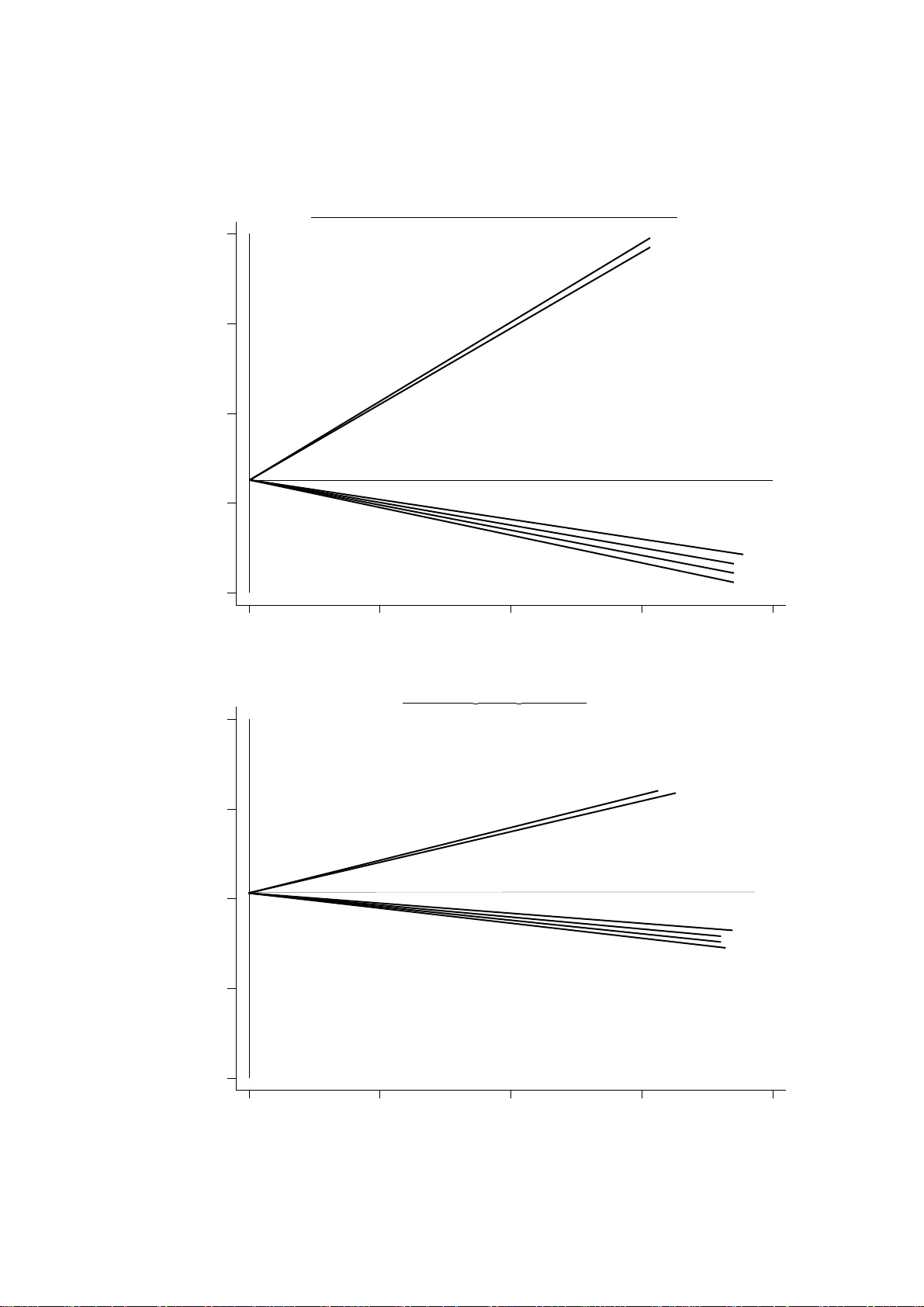
New E stimation P rocedur es for PLS Path Modellin g X. Bry Laboratoire LISE-CEREMA DE, Université de Paris IX Dauphine Email : bry xavier @yahoo.fr Abstract : Given R groups of numerical variables X 1 , ... X R , we assume that each group is the result of one underlying latent variable, and that all latent variabl es are bound together through a linear equation system. Moreover, we assume that some explanatory latent variables may interact pair wise in one or more equations. We basically consider PLS Path Modelling's al gorithm to estimate both l atent variables and the model's coefficients. New « external » estimation schemes are proposed that draw latent variables towards strong group s tructures in a more flexible way. New « internal » estimation schemes are proposed to enable PLSPM t o make good use of variable group complementarity and to deal with interactions. Appl ication examples are given. Keywords : Interaction effects, Latent Variables, PLS Path Modelling, PLS Regression, Thematic Components Analysis. Notations I n stands for identity matrix of size n . When the matr ix’s size is una mbiguo us, we’ ll simply wr ite it I . Greek lower case letters ( α, β, . ... , λ, µ, .. . ) stand for scalars. X is a data matrix describing n individuals (lines) using variables (columns). This symbo l indifferently stands for the variable group coded in the matri x. If variable group X contains J variables, we then wr ite : ( ) J to j j x X 1 = = . M is a sy mmet ric regular positive matr ix of size J used to wei gh X . Lo wercase x, y refer to column-v ectors of size n as well as to the corresponding variables. X 1 , ..., X r , ... , X R are R observed variable groups. Group X r has J r column s. M r is a sy mmet ric regular positive matr ix of size J r used to weig h variable group X r . Diag ( A,B,C ...) stands for the block-diagonal matr ix wit h diagonal blocks A, B, C ... < X > stands for the vec torial subspace spanned by variable group X . F and Φ stand for factors built up throug h linear combi nation of variables from group X . v, w stand for latent var iables (to be estimated thro ugh factors). The perpendicular projecto r onto subspace E will be writte n Π E . x being a ve ctor and E 1 , E 2 two subspace s, the E 1 -compone nt of x E E 2 1 + Π will be written x E E 2 1 Π (Note : the restriction of x E E 2 1 Π to subspace E 1 +E 2 is projector onto E 1 parallelly to E 2 ). If not explicitly mention ed, orthogonality will be taken w ith respect to the canonical euclidian metric I . Scalar product of two vec tors x and y will be writte n x y . Sy mbol ∝ stands for proportionnality of two vectors, e.g. : x ∝ y . Standardized variable x will be wr itten st ( x ). Juxtaposition of mat rices A, B, C ... will be wr itten [ A, B, C ...]. 1 A fe w acrony ms : PCA: Principal Compo nents Ana lysi s PLS: partial Least Squares PLSPM: PLS Path Modelling N.B. Variables are sy stematically assu med to have zero mean . 1. Intr oduction Conceptual models Consider a variable group Y describing an aspect of reality (e.g. Health) on n units (e.g. countries) and R explanatory variable groups X 1 , ... X R , each pertaining to a theme, i.e. havin g a clear conceptual unity and a proper role in the explanation of Y (e.g. Wealth, Education...). We may g raph the dependancy of Y on X 1 , ... X R as show n on fig ure 1. Figure 1 : Conceptual model X 1 X R : : Y X : : H e a l t h W e a l t h Ed u c a t i o n It should be clear that such a conceptual model shows no interest in the global relation between Education and Health over t he units, for instance, but aims at knowing wh ether, Wealth level etc. remaining unchanged , a change in Education implies a change in Health. So, arrows in this graph indicate marginal (or partial ) effects, and not global relations between each X r and Y . This analytical approach (the mutatis mutandis et ceteris paribus question) is the whole point of such models, so we think estimation strategies should reflect full conce rn of it. Modelling w ith Latent Variables • Consider R variable groups X 1 , ..., X R . One may assume that underly ing each group, there i s one l atent (unobserved) variable v r , and that these latent variables are linked through a linear m odel having one or more equations (cf. fig . 2). We shall refe r t o this mode l as the latent model . Figure 2 : Multi-equati on latent variables model X r v r Late nt mod el 2 • Consider a sing le equation latent model, in which q latent variables act upon one observed or latent variable. W e shall call the model a q -predictor-group one. A 1-predictor group model is essential ly different from a multi -predictor group one, i n that the effect of a predicto r group on the dependant group indicates a global relation in the former model, and a partial relation (controlling for all other pre dictor groups) in the latter model. • Each latent variable underlying a group of obs erved variables should, as far as possible, represent a group's strong structure, i.e. a component common to as many variables as possible in the group. At the same time , the latent variable set should fulfill, as best as possible, the latent model. It is easily understandable that these two constraints will gene rally draw the estimation in divergent directions. Ther efore, a compromise must be found. It also stands to reason that the estimation of a l atent variable with exclusive regard to the observed variables in its group, leaning on global redundancy between them, should make use of simple correlations (as PCA does), whereas its estimat ion with regard to the latent model, having to deal with effec t separation, should use partial correlations. One therefore ends up with two different estima tion schemes, and has to make them work h and in hand. • In multi-predictor group models, the question of collinearity between groups arises. We t hink that, from the mome nt this ty pe of model has been chosen by the analy st, he should not tolerate collinearity betw een groups, at least as far as strong within- group structures are concerned : the purpose of the model being to separate t he explanatory group effects on t he dependant one, these effects must indeed be separable. S o, within- group collinearity should be no problem, whe reas between -group collinearity should be one. 2. PLS Path Modelling's algorithm • This approach was initially pro posed by H. W old [ Wold 85], and improved by Lohm öller [Lohmöller 89]. Wold's algorith m supposed that the sig n of the correlation betwee n each dependant latent variable F r and each of its latent determina nts F m was know n a priori . This is a costly assumption. Lohmöller' s method notably relaxes this hypothes is [Lohmöller 1989][ Tenenhaus 1998][Vivien 2002], and carries out estimation without any more informat ion than the conceptual model we have presented here (i.e. mere dependancy arcs between variables). Therefore, let us here present Loh möller's algorit hm. • Consider R variable groups X 1 , ..., X r , ... X R . All variables are standardized. One make s the follow ing hy potheses: H1 : Each group X r is essentially unidime nsional, i.e. is gener ated by one sing le latent variable v r . Each variable in the gr oup can thus be writte n k r r k r k r v a x ε + = , whe re k r ε is a centered noise uncorrelated wit h v r . H2 : Latent variables are linked together by such st ructural relations as : r r t t tr r v b v ω + = ∑ ≠ , where r ω is uncorrelated wi th the v t 's standing in the rightha nd side. Some of the tr b 's are a priori know n to be 0. Hy pothesis H2 corresponds to the causal relation graph between latent variables. A non-n ull tr b coefficient means that there is a causal arc oriented from v t towards v r . 3 2.1. The algorithm Step 0 (initialization) : A starting value F r (0) is determined for each latent variable v r , for instance by equating it to one of the variables of its group. We suggest t hat one start wi th the group's first principal component, since it embodies the g roup's « commu nality » . Step p : Phase 1 (internal estimation of each variable): One sets :         − = Φ ∑ ≠ r t t tr r p F c st p ) 1 ( ) ( (1) ... where st( x) mea ns standardized x , and coefficients c tr are computed as follo ws: 1 – When latent variable v r is to be explained by variables { v t }, coefficient s { c tr } will be equated to regression coeff icients of F r on { F t } ; 2 - When v r is an explanatory variable of v t , c tr will be equated to sin gle correlation ρ ( F r , F r ). Phase 2 (external estimation of each variable): The internal estima tion Φ r is drawn to wards strong c orrelation structures of group X r by compu ting: ( ) ) ( ' ) ( p X X st p F r r r r Φ = (2) Note that, all variables being standar dized, this form ula also reads :         Φ = ∑ ∈ j X x r j r x p x st p F r j )) ( , ( ) ( ρ End : The algorithm stops whe n estima tions of latent variables ha ve reached required stability. 2.2. Discussion • Algorit hmic struct ure: Phase 2 (external estimation) of the curre nt step draws each latent variable estimation tow ards a strong structure of its group using binary correlations between the internally estimated value of the latent variable and all observed variables of its group. We study properties of operato r X r X r ' and ge neralize it in next section. Phase 1 (internal estimation) is supposed t o bring the estimation of the latent variable closer to the relation it should fulfil with the others. And so it does, to a certain extent. But, according t o us, it does not fully comply wit h the partial correlation logic, and therefore does not make full use of group-compleme ntarity to optimize prediction. This point is developpe d further below. It seems to us tha t external and internal estimations, w hich we tr y to make meet, each ha ve their own log ic : - External estimation, in order t o draw each latent variable towards strong correlation structures with in the group, naturally uses sin gle bivariate correlation between the v ariables in the group. 4 - Internal estimation, on the contrary , tries to draw the l atent variables towards a linear explanatory scheme, i.e. to separate the effects of explanatory groups onto the dependant group. Its logic should therefore use partial correlation. Converg ence of internal estimat ion may be reached, as well as that of external estimation, but the two limits will generally remain distinct, s ince external estima tion F r pertains to < X r >, when internal estimation Φ r does not a priori . • I nternal Estimat ion scheme : Let us get back to coefficients c tr . Suppose the model has but one equation, predicting l atent variable v r linearly from laten t variables { v t }. The internal estim ation of F r will be:         − = Φ ∑ ≠ r t t tr r p F c st p ) 1 ( ) ( ... where coefficie nts { c tr } are regression coefficients of F r on { F t }. These coefficients are partial effects, t hus comply with the effe ct-separation logic. Now, c onsider the internal estim ation of each v t : ( ) ) 1 ( ) ( − = Φ p F c st p r rt t where: )) 1 ( ), 1 ( ( − − = p F p F c r t rt ρ When there is but one equation in the model, we see that internal estimat ion of each predictor is taken as the predicted variable itself. Should there be several equations and v t appear as predictor of several dependant variables v r , the internal estimation would compute a sum of these dependant variables (externally estima ted)wheig hed by their global correlation with F t . In any case, the estimatio n Φ t completely ignores the existence of other pre dictors of v r . The fact that coefficient c rt does not convey any idea of partial relation here seems rather problematic to us. Let us n ow develop an alternat ive approach to external and inter nal estimation. 3. External estimation - Resultants: 3.1. Linear resultants • X being a group of J standardized variables, and y a standardized variable, XX'y will be termed simple resultant of y on group X , and shortha nded R X y . We have already noted that: • More generally , let y be a numerical variable and X a group of J numer ical variables. Let M be a regular sy mmet ric positive J × J matrix weighin g X . We call variable XMX ’ y : resultant of y on group X weighed by M , and shorthand it: y R M X , . Matrix XMX ' is of course none other than that of M -scalar product of observation (row) vectors of X . We showe d that the resultant can be used to measure the concordance of y wit h X in two way s : its direction gives the dimension of this concordance in the group’s sub-space, and its norm ca n be used to measure the in tensity of the link [Bry 2001]. 5 ∑ = = J j j j x x y y XX 1 ) , ( ' ρ • Now, let + ∈ R α . Matrix XMX ' being sy mmetr ic positive, it can be powered with α . Let us wri te: y XMX y R M X α α ) ' ( , = (3) and call it the α - degree resultant of y on X,M . • In PLSPM, the simple resultant on group X is used to draw a current estimation of a latent variable towards a strong correlation structure of X . How does resultant y R M X α , draw y towards a strong s tructure of X , and what structure? Let G k be the standardized k -th principal component of X weig hed by M , and λ k be the corresponding eigenva lue. G k is the eigenvector of XMX ’ associated with eigenvalue λ k . So, it is also the eigenvector of ( XMX ’) α associated with eigenvalue α λ k . Therefore, we have : ∑ = k k k k M X y G G y R ' , α α λ = ∑ k k k k G y G α λ (4) So, y R M X α , can be viewed as a sum of y ’s components on X ’s principal component basis, each component being weighed by the factor’s structural force λ k (i.e. t he part of total variance it captures) taken with power α . As a consequence , y is drawn towards Principal Component s of X in prop ortion of the percentage of variance they capture (put to power α ), and of their correlation with y . • I t is easy to see on (4) that: - I f α = 0: y G y G y R X k k k M X > < Π = = ∑ 0 , . No account is taken of correlation struc tures in group X . - I f α > 0, heavier PC's wil l draw strong er on y (provided it has non- zero correlation with the m). - If α → +∞ , the heaviest PC with which y has non-zero correlati on becomes dominating in the sum, so that y is simply proj ected onto it. As a conclu sion, continuou s parameter α reflects the exte nt to which we con sider correlation structures in X . Figure 3 gives a little illustration of how resultants w ork. Here, we have, for simp licity' s sake, a bidimensional X group having P CA eigenva lues λ 1 and λ 2 such that λ 1 = 2 λ 2 (their mag nitudes are figur ed using a thick line). Variable y is positionned in plane < X >, as shown. Then, resultants y R X 1 t o y R X 3 are computed, y R X 0 being obvious ly equal to y . Figure 3: How resultants work λ 1 λ 2 y = R 0 X y R 1 X y R 2 X y R 3 X y 6 • The purpose of matrix M is also to modu late the account take n of correlation structures in X , y et it works a bit differently : l ess smo othly , in a sense, but allowing to di stingu ish sub-g roups in X . Of course, if we t ake M = ( X'X ) -1 , we e nd up with: ( ) ( ) y y y X X X X y R X X M X > < > < − Π = Π = = α α α ' ) ' ( 1 , (which we will also wr ite: y R X > < ) ... i.e. the same resu lt as when α = 0 whate ver M . But let us now partiti on X into R sub-g roups X 1 , ..., X r , ... X R and let M = Diag ({( X r 'X r ) -1 } r ). Then: ∑ ∑ > < − Π = = r X r r r r r M X y y X X X X y R r ' ) ' ( 1 , One sees that n o account is taken of correlation struct ures within sub-groups, correlations between sub- groups still being cons idered. The immedia te application of that is to deal with categorical variables. Suppose we have a group X of R categ orical variables. Each such v ariable X r will be coded as the dumm y variable set of its value s. Within this set, correlation structur es are irrelevant. So, this set will be regarded as a numer ical variable sub-g roup and one will us e M = Diag ({( X r 'X r ) -1 } r ). When a nume rical variable group X is partitionned into R sub- groups and one wan ts to take correlation structures into acc ount within each as well as between t hem, bu t balance the contribution of groups to the resultant, one may use M = Diag ({ w r I Jr } r ), where J r is the nu mber of variables in g roup X r and w r a suitable weig ht, for instance th e inverse of X r 's fir st PCA eigenva lue, as in Multiple Factor Ana lysi s [Escofier, Pagès 1990]. 3.2. Non-linear Resultants 3.2.1. Why may one want to go beyond linear resultants? Consider a group X of standardized numer i cal variables, weig hed by mat rix I . We have seen that, for α > 0, α I X R , operator will alwa ys dr aw variable y harder towards stronger PC' s (with which it has non- zero correlation), even - and this is the point - if y is ve ry far from them, i.e. the se correlations are very low. This can be seen on fig ure 3: y is closer to the second PC, and yet is drawn towards the f irst one. Under the hy pothesis that group X is fu ndamen tally un idimens ional (H1), this is nothing to complain about. But ma ny situation s are thoroughly multidim ension al. Let us just recall, for History 's sake, the gr eat Spearman- Thurstone controversy as to the dimens ions of intell igence. Spearman, and th ose who fo llowed him, were misla id for 30 years by the prejudice that there was but one factor underly ing intellectual aptitudes. Thurstone pointed out the existenc e, among the psycho metric test data, of several positively but weakly correlated variable bundles, and made clea r that it was esse ntial that PCs help identify them. Comp uting seve ral PCs instead of one is a f irst considerable improveme nt. The second improveme nt owed to Thurstone is the rotation he proposed of original PCs so as to make the m adjust variable bundles (yet, it may still not be suffi cient, as mu tually uncorrelated component s cannot adjust correcly to correlated bundles). In our external esti mation context, w e wou ld like to « draw the e stimation to wards a close structural direction » (e.g. bundle, if any ), still pay ing some respec t to the strengt h of this structure . It is clear that the linear resultant fa i ls to achieve that. Consider f igure 4, showi ng a group consi sting in tw o positively but wea kly correlated variable bundles of equal struc tural importance. 7 Figure 4: Bundles, PCs and resultants Bund le A’s d ir ect io n Bun dle B ’s dir ec tion 1st PC 2nd P C y R X y B A Variable y is close to bundle A, and has ve ry little to do with bundle B (which i s only w eakly correlated with A). Yet, the resul tant draws it tow ards the firs t PC, and so, towards B . Let us rotate the PCs so a s to make each one as close as possible to a bundle, and substit ute them for gr oup X in the resultant comp utation. As these rotated PC's capture the sa me amoun t of variance (for obvious sy mmetry reasons) and are uncorrelated, the resultan t operator will boil dow n to the identity matrix, and will leave a ny variable y unc hanged (fig. 5). So, y is still not draw n towards the closest structural direction. Figure 5: Bundles, rotated PC's and resultants A B ro tat ed P C y=R PC y rot ate d PC To achieve that, we have to introduce some bonus to « closenes s » in the resultant' s computation, and this make s it non-lin ear. 3.2.2. Non-linear resultants a) Formulas • The simple resul tant of y on a numer ical standardized variable group X was calculated as follo ws: ∑ = j j j X x x y y R Taking β ∈ R + , we may introduce a bonus to closeness by calculating in stead: ∑ j j j j x x y x y β It may be suffic ient, in practice, to take β = 2 k , where k is a natural in teger, which we sh all refer to as the resultant' s order . Then, we wr i te: ∑ + = j j k j k X x x y y S 1 2 , ) ( 8 • L et us generalize the previous situation by considering a numerical variable group X partitionned into R sub-g roups X 1 , ..., X r , ... X R and let M = Diag ({( X r 'X r ) -1 } r ). The linear resultant was: ∑ > < Π = r X M X y y R r , Now, if we introduce our bonus to closeness in the sa me wa y a s above, we have: ∑ ∑ > < > < > < Π Π = Π > < = r X k X r X r k k X y y y X y y S r r r 2 2 , ) , ( co s ) ( (5) This formul a generalizes the previou s one and allows us to deal with ca tegorical variables. It can obviously be written : y X XM y S k y X k X ' ) ( , , , = (6) ... where { }       Π = − > < r r r k X k y X X X y Diag M r 1 2 , , ) ' ( is a sy mmet ric positive matrix including the « bonus to closeness » effect and thus, depending on y (hence the non-linearity ). Matrix M X,y,k is a local euclidian metric matri x. So, matrix ' , , , , X XM S k y X k y X = is a local resultant operator. Just as linear resultant operators, it can be put to any positive po wer α ∈ R + : ( ) α α ' , , , , X XM S k y X k y X = (7) As w ith li near resultants, α can be interpreted as the degree of account taken of struc tures in X . b) Behaviour When α = 0, we get t he orthogonal projection onto < X >. Now, let us take α > 0: When k = 0, we g et the linear resultant back, the bonu s to closeness being nu ll. When k > 0, variable subgroups spann ing subspa ces closer to y are given more we ight. When k → ∞ , the variable subgroup spanning the closest subspace to y is dominating: ) ( , y S k X α is colinear to y 's proje ction onto this subspace. When sub-groups are reduced to single variables, ) ( , y S k X α ends up being colinear to the variable best correlated with y . Let us illustrate this with an example. Using a random number generator, we computed a variable group X consisting in 2 numerical variable bundles ( A and B ) appr oximately makin g a π /4 angle. Bundle A contains 4 variables ( a 1 , ... a 4 ) obtained by adding a little random noise to the same variable. Bundle B only contains 2 variables ( b 1 , b 2 ), generated in the same way . Bundle B i s thus « lighter » than A . Then, several y j variables are generated through l inear combination of variables in X . Finally , we computed non-linear resultants of y j 's on X wit h k ranging from 0 to 6. Resultant ) ( 1 , y S k X will be shorthanded S k y . Figur e 6 shows what becomes of a variable ( y 7 ) located inbetween bundles A and B , but closer t o B , according to the k value (all variables are projected onto X 's f irst PCA plane). 9 Figur e 7 shows n l-resultants for all variables and k -values 0 (linear resu ltant) and 6 (furiously no n-linear resultant). I t is easy to notice that S 6 resultant s are grouped in the bundles' ne ighbourhoods, in contrast wi th S 0 ones. Variables y 4 , y 5 and y 7 have been draw n by S 6 towards bund le B , whereas y 1 , y 2 , y 3 and y 6 have been drawn towards bundle A . Figure 6: possible attractions of an « inbetw een » variable Figure 7: S 0 and S 6 resultants 10 CorF2 CorF1 0 .987106 -.270801 .59072 a1 a2 a3 a4 b1 b2 S0y7 S1y7 S2y7 S3y7 S4y7 S5y7 S6y7 y7 CorF2 CorF1 0 .989949 -.953942 .888049 S0y1 S0y2 S0y3 S0y4 S0y5 S0y6 S0y7 S6y1 S6y2 S6y3 S6y4 S6y5 S6y6 S6y7 a1 a2 a3 a4 b1 b2 y1 y2 y3 y4 y5 y6 y7 c) Link with the quartim ax rotation A link may be established between 1 st ord er non linear resultant and quartimax rotation. This rotation aims at drawing a set of H orthogonal standardized factors closer to H variable bundles. This method has been derived by several authors ([ Ferguson 1954] [Carroll 1953] [Neuhaus & W rigley 1954] [Saunders 1960]) from di stinct but equivalen t criteria. For instance, it can be derived from the followin g program: ∑ ∑ = H h j h j F F F x Max H 1 4 ed standard iz orthogonal ,..., ) , ( cos 1 Keeping the heuristic base of the program, w e can extend it to any even power greater than 4. Thus, for k ≥ 2, we g et: ∑ ∑ = H h j h j k F F F x Max H 1 2 ed standar diz orthogon al ,..., ) , ( cos 1 This program can be rew ritten: ∑ ∑ = − H h h j j h j k F F F x F x Max H 1 1 2 ed s tandar diz orth ogon al ,..., ) , ( cos 1 That is: ∑ = − H h h h k X F F F F S Max H 1 1 , ed s tan dard iz orth ogona l ,..., ) ( 1 In every scalar product < S X , k -1 ( F h ) | F h >, two eleme nts are taken in to account: the correlation of the factor wit h its non- linear resultant, and the n orm of that res ultant. The non-linea r resultant dra wing a f actor F towards a « strong and close » structure, the factor itself wi ll be all the closer to this structur e as it is correlated to the resultant. On the other hand, the resul tant's norm will be all the greater as F is close to the structure. Thus, the criterium maximi zed by the progr am is straigh tforward to interpret. 11 4. Internal estimation We are now going to set up an alternative internal estimatio n scheme . Let us take back notations from §2. External esti mates of latent va riables will be referred to as factors . 4.1. Latent model without interaction effects 4.1.1. Single equation m odel Take latent model: r r t t tr r v b v ε + = ∑ ≠ . External estimates of v r , v t computed at step p -1 are F r ( p -1), F t ( p -1). Indices r and t will refer to dependant and explanatory variables respectively . Let F -t stand for the the set of all explanatory f actors except F t . Estim ation formulas: • To estimate v t , we have to take into account all other predictors of v r , and shall take advantage of the whole prediction potential of group X t . So, we regress F r ( p -1) onto { X t , F -t ( p -1)}, and take the component on X t of the prediction. So, we ha ve: ( ) ) 1 ( ) ( ) 1 ( − Π = Φ > − < > < − p F st p r p F X t t t (8) • We could keep estimating v r internally using Lohmöller' s method, i.e. formu la (1), { c tr } being the coefficient s of F r ( p -1)'s regressio n upon { F t ( p -1)}. Geometrically speak ing, we would t hen have: { } ( ) ) 1 ( ) ( ) 1 ( − Π = Φ > − < p F st p r p F r t t In fact, we woul d like, just as for the explanatory variables, to get an internal estimation of v r that is in < X r >, in order to be able to skip external esti mation. So, we s hall take: { } ( ) ) 1 ( ) ( ) 1 ( − Π Π = Φ > − < > < p F st p r p F X r t t r (9) Properties: • Formu la (8) uses partial relations between dependa nt and explanatory variables. • As each variable v r 's internal estimat ion now pertains to subspace < X r >, it becomes possible to skip external estima tion in the PLSPM algorithm. The roles of internal and external estimations are well separated: internal estima tion's purpose is to maximize latent model adjustment, whe reas external estimation' s purpose is to draw estima tions towards g roups' strong structures. • Notice that (8) maximis es coefficient R² over < X t >, given F -t . If we iterate (8) to internally estimate in turn all explanatory variables v t , R² increases throughou t the process. Formula (9) can only increase R² too. So, if we s kip external esti mation, R² can only i ncrease throug hout the PLSPM algorithm . • Now, let us regress F r ( p -1) onto all explanatory groups, i.e. X , where X = [ { X t } t ], and let ) 1 ( − p F r t be the < X t >-compo nent of t he prediction. If we replace every current explanatory factor F t ( p -1) by ) 1 ( − p F r t , then regressing onto { X t , F -t ( p -1)} amounts to the same as re gressing on X , and theref ore, (9) yields: 12 ( ) ) 1 ( ) ( − = Φ p F st p r t t and of course, (8) gives: ) 1 ( ) ( − = Φ p F p r r . So, we ha ve a fixed point of the alg orithm. • If there is but one explanatory group X t , and we skip external estimation, the algorithm will perform canonical correlation analysis. Indeed, once stability is reached, the estimated variables verify the following characteristic equations: ( ) ) ( ) ( ∞ Π = ∞ > < r X t F st F t and ( ) ( ) ) ( ) ( ) ( ) ( ∞ Π ∝ ∞ Π Π = ∞ > < > ∞ < > < t X r F X r F st F st F r t r If we add up standard external estimation using si mple resul tants, we ge t rank 1 factors of PLS regression. But again, the thing to focus on is the use of partial relations to predicto rs in the estimatio n process when there are several predictor groups. Illustration of the main difference with Lohm öller's procedure Consider the case reported on figure 8. Here, we have a dependant group reduced to a sing le variable y , t o be predicted from two groups X 1 and X 2 . Explanatory group X 1 contains standardized variables a and b , which are supposed to be uncorrelated, while X 2 m erely contains c . The only latent variable to be estimated is v 1 i n group X 1 . The dependant variable y pertains to plane < a,c >, and is such that its orthogonal proj ection onto < X 1 > is colinear to b (i.e. y = < a,c > ∩ < b, ⊥ > ). The dimen sion in X 1 that is the most us eful, together with c , to predict y is therefore a . Whatever the initial F 1 value, Lohmöller' s procedure will i nternally estimate v 1 as y = Φ 1 . Then, external estima tion will replace it with b y y X X F X = Π = = > < 1 ' 1 1 1 (once standardized). We can see that we have reached stability . Figure 8 y X 1 X 2 a b c In contrast, the procedure we sugg est, proj ecting y onto < X 1 > parallelly to c , will find a = Φ 1 . Then, external estima tion will replace it with a a a X X F X = Π = = > < 1 ' 1 1 1 . Here also, we ha ve reached stability. Collinearity problems: • Let a be a linear combination of F -t factors. We have: 0 = Π > < > < − a t t F X . S o, (8) ensures that Φ t is as far as possible from collinearity with F -t . Of course, r F X F t t > < > < − Π is uniquely determined only if < X t > ∩ < F -t > = 0. This will be the case in practice, provided group X t is not too large (with respect to the number of observations) . If it is, one possibility consists in reducing its dimen sion through prior PCA. W e regard it as a good one, 13 because really weak dimension s should any way be discarded, and using a subspace of < X t >, we keep Φ t in < X t >. A rema ining collinearity probl em betwee n < X t > and < F -t >, once the weaker dimen sions in < X t > removed, woul d indicate that X t shares strong explanatory dimens ions with the ot her explanatory groups. Thi s is a problem, but less w ith the method than w ith th e conceptual model: this m eans in deed that the partial effects of explanatory g roups upon the dependant one can theoretically not be separated, whi ch violates the funda mental assumption of our analytical approach. Under such circumstance s, how could one think of an explanatory model? • Whe n there is some collinerarity wit hin X t , r F X F t t > < > < − Π ca nnot be expressed uniquely in terms of j t x variables. Nevertheles s, if < X t > ∩ < F -t > = 0, r F X F t t > < > < − Π exists and is unique, w hich is enoug h for our estimation metho d (it could be computed us ing X t 's PCs). So collinearity with in X t causes no rea l pro blem. 4.1.2. Multi-equation m odel • Here, we suppose that the model contains several equations. A latent variable v r can be the dependant one in some equations, and explanatory in ot hers. Supposing v r intervenes in Q equations.We may apply formulas (8) and (9) to estimate se parately v r in each equation. Equation q leads to internal est imation ) ( p q r Φ . How can we sy nthesize a unique internal estimation from all these separate estimat ions? Let ) ( p r Ω = { } q q r p ) ( Φ and α > 0. A simple and na tural way is to set ) 1 ( ) ( ), ( − = Φ Ω p F R p r I p r r α , for instance. • In what follows, we will refer to this PLSPM algorithm as the Thematic Components PLS Path Modelling (shorthande d TCPM). The reason for this being that the idea of projecti ng the dependant variable onto each explanatory group parallelly to all other explanatory factors was firs t developped in an algorith m called Thematic Components Analysis , dealing with a single equation m odel [Bry 2003]. 4.1.3. Application example: the Senegalese presidential election of 2000 The election of the Senegalese president has two ballots. The two candidates who g et the highest scores in the first ballot are the only ones to compete in the second ballot. The winn er is the one who wins the relative majority i n the second ballot. The data : (cf. appendix A) Senegal is divided i nto 30 departments. We shall try to relate t he departemental scores of the candidates to economic, social and cultural characteristics of the departments, using the conceptual model shown on figure 9. The rationale behind this model, is that : 1) Concerning the first ballot, the economic and social situation should be an important factor of pol itical choice. Besides, in a given socio-econom ic situation, cultural considerations such a ethnic and religious background ma y still cause differences in the vote. 2) The results of the second ball ot are mainly determined by those of the first, through a strong vote-transfer mecha nism. 14 Figure 9 : conceptu al model for the senegalese elections X 1 = E c o no m i c , So c i a l & D e m o g r a p h i c B a c k g r o u nd X 2 = E t hn ic & R e li g io u s B a c k g r o u nd X 3 = 1 s t B a l l o t sc o r e s X 4 = 2 n d B a l lo t sc o r e s The model has tw o parts : (a) X3 = f(X1 , X2) and (b) X4 = f(X3). The latent variable in group Xk wil l be written Fk . The variables used in this a naly sis are : Group X1 (economic social and demographic background) : NHPI : Normalized Hu man Poverty I ndex (a compound measu re of educational, sanitary and life conditions indicators) PctAgriInc : Proportion of the global income that is mad e in Agric ulture IncActivePers : Averag e Income of an active person ActivePop : proportion of the active persons in th e population. Scol : Gross Enrolmen t Ratio Malnutrition : Malnutrition rate. DrinkWater : Proportion of population having a ccess to drinkable water. Rural , Urban : Percentages of rural and urban populations. PopDensity : Population Density HouseholdSize : Averag e number of persons in a household Pop0_14 , Pop15 _60 , PopOver60 : Proportions of population aged 0 to 14, 15 to 60, and over 60. WIndep , WPu blic , Wprivate , WApprentice : Proporti ons of employ ed population working as independant wor ker, Public Sector Salaried worker, Private Sector Salaried worker, and Apprentice. OEm ployed , OUnemploye d , OStudent , OHouseWife , ORetired : Prop ortions of population being : employ ed, unemploy ed, student, house wife, retired. ASPrim , ASSec , ASTer : Activi ty Sectors ; respectively P rimary , Secondary and Tertiary. Group X2 (ethnic and religious background) : Wolof , sereer , joola , pulaar , manding : Percentage s of the main e thnic groups. Moslims : Percentage of mo slim population. Group X3 (1 st ballot scores) : Thiam1 , Niasse1 , Ka1 , Wade1 , Dieye1 , Sock1 , Fall1 , Diouf1 , Abstention1 : Departmental scores of candidates, and abstention. Every candidate s core is calculated as number of votes for the candidate over number of electors on the official list. Group X4 (2 nd ballot scores) : Diouf2 , Wade2 , Abstention2 . 15 We must mention that candidates Thiam, Dieye, Sock and Fall most generally had very low scores at the first ballot (below 1%), and therefore had very little weig ht in the coalitions that formed between the two ballots. Atten tion should thus be focussed on the other candidates (Wade, Diouf, Niasse, Ka). TCPM results: We thought m ore careful to first inve stigate equations (a) and (b) separately , and check the closeness of estima tions for the comm on latent var iable F3 , before launchin g the joint estimat ion of the who le 2-equation sy stem. Stability (changes lo wer than 1/1000) was alway s reached in less tha n 10 iterations. Separate estimations of equations (a) and (b) We successively used resultants S 0 , S 1 , S 2 , S 3 , S 4 to see whethe r adjustment could be improved. Table 1 gives, for each S -choice, the R² coe fficient for equations (a) and (b) estimated separately , as well as t he correlation betwee n the two e stimations of the F3 factor. Table 1: Separate estimation adjustment qualit y according to S-choice S operator R² equation (a) R² equation (b) Corr (F3(a),F3(b)) S 0 .686 .912 .897 S 1 .711 .925 .913 S 2 .669 .895 .914 S 3 .658 .864 .849 S 4 .653 .821 .767 All in a ll, the choice of S 1 seems best, as it gives better adjustmen t of both equations, and (almo st) the best correlation between F 3 estimations. Suc h a good correlation will en title us to proceed later on to a joint estima tion of both equations. Interpretation of equation (a) estimated on its own : Compari ng the factors gi ven by the dif ferent S order options, we no ticed that S 1 ,... S 4 give out very close results (correlations betwe en estima tions of the « same » factor ranging from 0.97 to 1), but that there are more im portant differences betw een the resu lts given by S 0 and S 1 , especially in g roup X2, as shown be low. Factor F 1 F2 F3 correlation between S 0 - and S 1 -esti mations .994 .491 .815 Considering this, we found impor tant to interpret results in the S 0 and S 1 cases. • F3 factor was r egressed on F1 and F2 , which g ave the followi ng resu lts : S = S 0 : R² = .686 Explanatory f actor → F1 F2 Coefficien t .632 -.434 P-value 1 .000 .000 1 Critical P. values shou ld not be used for inference, but only be taken as a descriptive indicator. 16 S = S 1 : R² = .711 Explanatory f actor → F1 F2 Coefficien t .776 .304 P-value 1 .000 .007 • I nterp retation of F3 : F3- Correlations Thiam1 Niasse1 Ka1 Wade1 Diey e1 Sock1 Fall1 Diouf1 Abst.1 S = S 0 : .226 .467 -.596 .730 -.633 -.542 .334 -.553 -.383 S = S 1 : .148 .071 -.416 .975 -.277 -.243 .150 -.729 -.263 Let us con sider the candidates having non-skin ny scores. S = S 0 : Factor F3 opposes MM. Wade and Niasse to MM. Diouf and Ka. Note that after t he first ballot, candidates Diouf and Ka formed a conservative coalition, wher eas candidates W ade and Niasse formed a coalition to « change » (« Sopi » , meaning « change » in wolof, wa s their slog an). S = S 1 : Here, factor F3 opp oses M. Wade to M. Diouf, and to a modest extent, M. Ka. The correlation with M. Wade's score is much highe r, but M. Niasse has been lost on the wa y . • I nterp retation of F1 : F1-Correlations NHPI PctAgriInc IncActivePers ActivePop Scol Malnutritio n DrinkWater Rural Urban PopDensity HouseholdSize Pop0_14 Pop15_60 S = S 0 : -.937 -.437 .713 -.294 .725 -.021 .688 -.956 .956 .767 -. 086 -.720 .732 S = S 1 : -.942 -.451 .730 -.285 .672 .045 .714 -.960 .960 .781 -. 050 -. 733 .774 PopOver60 WIndep WPublic Wprivate WApprentice OEmployed OUnemployed OStudent OHouseWife ORetired ASPrim ASSec ASTer S = S 0 : -.320 -. 564 .931 .963 -.700 -.834 .870 .607 . 513 -.097 -.956 .914 .940 S = S 1 : -.385 -. 615 .944 .968 -.656 -.815 .885 .543 . 543 -.141 -.955 .906 .942 From these correlations, it is clear that in both cases, F1 opposes urban depa rtments (high values) to rural ones (low values). Urban departments have a higher population density , are better provided with indus try and services and are relatively rich, wher eas rural ones merely depend on agriculture and are very poor. • I nterp retation of F2 : F2- Correlations Wolof Sereer Joola Pulaar Ma nding Moslims S = S 0 : -.469 -.628 -.271 .907 .428 .316 S = S 1 : -.225 -.011 .949 -.534 .076 -.878 17 S = S 0 : Factor F2 is highly correlated with th e presence of the Pulaar ethnic group. S = S 1 : Here, factor F2 is high ly cor related posi tively with the presence of the Joola ethnic group and nega tively with the proportion of moslims in the population. Recall that the great majority of the Joola people lives in the south deparment s and is christian, and that most christians are J oolas, too, hence an interdepartme ntal correlation of -.839 between t he percentage of Joolas and that of mosli ms. In this case, the choice of S has heavy consequences: the computed factors do not quite seem to poi nt to the same p henomeno n, and will not lead to identical mode ls. • We end up with the followi ng model s, relating standardized factors: S = S 0 : F3 = .632 F1 - .434 F2 (R² = .686) S = S 1 : F3 = .776 F1 + .304 F2 (R² = .711) If we select the variable best correlated with the f actor in each group, we ha ve: S = S 0 : Wade 1 = .204 PctUrban - .053 Pulaar + . 119 (R² = .595) (P) (0.0 00) (0.193) (.000) S = S 1 : Wade1 = .215 PctUrban + .107 Joola + .094 (R² = .646) (P) (0.0 00) (0.021) (.000) Note that regression of W ade1 onto PctUrban alone gives R² = .568. The Pulaar factor does not seem to have a signi ficant role in the mode l of Wade1 , whereas t he Joola factor has, and provides a better predi ction. If we try to model the variable the most negatively correlated with F3 in the case S = S 0 , i.e. M. Ka 's score, we f i nd: Ka1 = .000 PctUrban + .117 Pulaar + .015 (R² = .395) (P) (0.994) (0.000) (.288) So, the use of S 1 and S 0 has directed us towards two different phenomeno ns: the urban factor and the J oola region' s bonus in the W ade vote ( S 1 ), and t he Pul aar factor i n the Ka vote ( S 0 ). But the first phenome non is globally mo re important, and wa s more c learly set out. Interpretation of equation (b) estimated on its own : Here, the choice of S does not lead to very different results. W e s elected S = S 1 , since it provides the best adjusted latent model. • I nterp retation of F3 : Correlations Thiam1 Niasse1 Ka1 Wade1 Dieye1 Soc k1 Fall1 Diouf1 A bst.1 F3 .307 .230 -.670 .865 -.275 -.130 .283 -.803 -.046 F3 opposes the Wade liberal vote t o the conservative socialist vote represented by MM. Diouf and Ka . • I nterp retation of F4 : Correlations W ade2 Diouf2 Abst.2 F4 .921 -.955 -.126 F4 opposes final Wade and Diouf votes. 18 • The estimated laten t model is: F4 = .962 F3 ( R ² = .925) Selecting the observed scores best correlated with the factors and relevant with political orientations, we easily get to the following model of the final Diouf score, expressed as a function of his former score and t hat of his 2 nd ballot ally, M. Ka: Diouf2 = .944 Diouf1 + .786 Ka1 - .025 (R² = .935) (P) (.000) (.00 0) (.174 ) It is also possible to model the fina l Wade score i n the sam e way , with near ly equivalent qual ity. Joint estimation of equations (a) and (b): We know enoug h, by now, about the two « conceptual equations » ( economic & cultural → vote1 and vote1 → vote2 ) to try and match t hem thr ough the joint estim ation process. Table 2: Joint estimation adjus tment quality accordin g to S- choice S operator R² equation (a) R² equation (b) S 0 .655 .861 S 1 .648 .843 S 2 .642 .746 S 3 .655 .713 S 4 .662 .684 As sh own on table 2, the best latent model global adjustment quality w as obtained for S = S 0 , but results gi ven by S 0 and S 1 are rather close. Besides, when correlating F2 estimations, one can notice a drastic change in F2 when one leaves S 0 or S 1 for S 2 or a higher order S . So, we may feel important to present S 0 - and S 2 - estima tions. Factor interpretation : F1 has exactly the same interpretation as i n the separate estima tion ( rural / urban ). So has F4 ( Wade2 / Diouf2 ). As for F2 and F3, S 0 leads to the same phenomenon as in the separate estimation ( Pulaar factor in the Ka vote), wher eas S 2 leads to the phenomenon outlined by S 1 in t he separate estimation ( urban factor and Joola bonus for W ade ). Final mod els : We end up with two possible models, of unequal adjustment quality , but poi nting out different and equally interesting phenome nons. If we select the one or two best correlated variables with each factor, we g et: S 0 → Model 1: Urban , PctPulaar → Wade 1 (Ka 1) Wade 1 (Ka 1) → Wade 2 (Diouf 2) 19 S 2 → Model 2: Urban , PctJoola (PctMoslims) → Wade 1 (Diouf 1) Wade 1 (Diouf 1) → Diouf 2 (Wade 2) Combin ing these two models gives our final path model of the contest (fig. 10). All coefficients have P-value below .01 except for the Joola effect in Wade1's mo del (P = .02). Figure 10: final path model of the electoral contest Economic Ethnic / Religious 1st ballot 2nd ballot Pct Urb an Pct Pu la ar Pct J ool a Dio uf Ka Wade Diou f Wad e .126 .117 .215 .107 .944 .786 - .778 .638 R²=.319 R²=.395 R²=.646 R²=.935 R²=.688 It is clear t hat the use of different S -degrees has allowed us to approach the data with more deli cacy , and that the fina l model better reflects the complexity of the studied reality . 4.2. Dealing with interaction eff ects So far, we only considered the predictors' marginal (constant) effects on the dependant variable. Let us now release this cons traint by allowi ng a predictor's effect to be a linear func tion of other predictors' values. 4.2.1. Single equation m odel with interaction effects 4.2.1.1. The mod el Consider the fol lowing single equation mod el, in wh ich a predictor interacts with some others: ∑ ∑ ∑ ≠ ∈ ∈ ∈ + + + = t u J E F u u t J F r rt t J F r r s t s s u s t r t s r F F F F F \ ) ( β δ β β F s is the dependant variable. The set of its predictors is E s . Among st them , F t i nteracts wit h some other predictors, whose set i s denoted J s t . Supposing that all variables are currently known but F t , we have to extend our internal estimation procedure so as to estimate F t (internal esti mation wil l be denoted Φ t , as before). Note: Should the model contain some interactions that do not involve F t , each of the interac ting predictors and of their products could be considered as part of the F u 's in the last summ ation. 4.2.1.2. Internal estim ation procedure for interactive latent variables Notation: F being a variable and X a variable group, F ⊗ X (or X ⊗ F ) will refer to the group formed by multi plyi ng F with every x j in X : F ⊗ X = { Fx j | x j ∈ X }. 20 Algorit hm: Initialization: Φ t 's initial value is calculated as if all δ rt coefficients were zero, i.e. using the interna l estimatio n sche me we proposed in section 4.1. for an explanatory f actor. Current step 1: Regress F s onto { } t s r J F t r s F E ∈ Φ ∪ . This provides with a current estimation of coefficients β t and δ rt ,denoted: rt t δ β ˆ , ˆ . Current step 2: 1) C alculate group Y t = t J F r rt t X F s t r ⊗ + ∑ ∈ ) ˆ ˆ ( δ β and use it as a new group in the internal estimation, to determine a factor G t . This mea ns regressing F s ont o Y t , F r and all non-interactive predictors , and extracting th e Y t -compone nt G t . 2) Then, divide G t by ) ˆ ˆ ( ∑ ∈ + s t r J F r rt t F δ β and standardize the result. This provides the new current value for Φ t . If this value i s close enough fr om the previous one, stop. Else, go back to current step 1. The illustration of thi s algorithm is given on fi gure 11 in a simplifi ed case. Figure 11: Internal estimation of an i nteractive variable F s Φ t F r Φ t ( β t + δ rt F r ) Φ t β r F r < X t > < F r ⊗ X t > ^ ^ ^ F r Dependant factor F s has only two predictors F r and F t , which interact. We illustrate F t 's internal esti mation. Current step 1 F s is regressed on F r , Φ t and F r Φ t , whic h give s estima ted coefficients rt t r δ β β ˆ , ˆ , ˆ . F r F s G t < ( β t + δ rt F r ) ⊗ X t > ^ ^ Current step 2 1) Subspace t r rt t X F ⊗ + ) ˆ ˆ ( δ β is formed. Then, F s is regressed on this s ubspace and F r , whic h give s a new com ponent G t . 21 F r F s Φ t F r Φ t < X t > < F r ⊗ X t > ( β t + δ rt F r ) Φ t ^ ^ 2) From equation t r r t t t F G Φ + = ) ˆ ˆ ( δ β , we draw the n ew va lue of Φ t (so, that of F r Φ t ). Properties: • R² increa ses: Curren t step 1: The standard multiple reg ression optimizes R². Curren t step 2: Subspace > ⊗ + < ∑ ∈ t J F r rt t X F s t r ) ˆ ˆ ( δ β contains the solution of step 1: t J F r rt t s t r F Φ + ∑ ∈ ) ˆ ˆ ( δ β , but is larger. The regression performed here there fore increases R². • When no F t in X t does really interact with any other predictor in F s 's model, the procedure boils down to the formul a used for models w ithou t interactions: Curren t step 1 finds all 0 ˆ = rt δ . Therefore, subspace > ⊗ + < ∑ ∈ t J F r rt t X F s t r ) ˆ ˆ ( δ β formed in current step 2 is none other than < X t >. So step 2 amounts to repeating initialization, i.e. what is done in model s witho ut interactions. 4.2.2. Multi-equation m odel with interaction effects There is absolutely no dif ference with the techniq ue used when no interaction is cons idered. 4.2.3. First application exam ple: simulated data • For 100 observations, we generated 20 independant random variables using uniform distribution U [–1 , 1] , and aranged them in 2 groups, A and B , containing 10 variables each: a1 ... a10 for group A , and b1 ... b10 for group B . Then, we computed the follow ing c variable: c = 0.2( a1 + b1 )/ 2 3 / + 0.8( a2 / 10 + b2 /10 + a 2 . b2 )/ 53 450 / • All variables na turally ha ve zero mean, includi ng products ai.bj , since E( ai.bj ) = E( ai ).E( bj ) = 0. • Variable c can be written: c = 0.2 c1 + 0.8 c2 , where c1 = ( a1 + b1 )/ 2 3 / and c2 = ( a2 /10 + b2 /10 + a 2 * b2 )/ 53 450 / are two independant v ariables of unit var iance: ∀ i : V( ai ) = V( bi ) = (1+1)²/12 = 1/3 ; ∀ i,j : V( ai.bj ) = E( ai.bj )² = E( ai ²).E( bj ²) = V( ai ).V( bi ) = 1/9 ∀ i,j : Cov( ai , bj ) = 0 ; Cov( ai , ai.bj ) = E( ai . ai.bj ) = E( ai ² .bj ) = E( ai ²).E( bj ) = 0 Similar ly, Cov( bj , ai.bj ) = 0. 22 As a consequence: V( a1 + b1 ) = V( a1 ) + V( b1 ) =2/3 and: V( a2 /10 + b2 /10 + a 2 . b2 ) = V( a2 )/100 + V( b2 )/100 + V(a 2 . b2 ) = 53/450. Therefore: V( c1 ) = V( c2 ) = 1. • Note that coefficient of c1 in c is four times smaller than that of c2 . Variable c1 contains no interaction betwee n a1 and b1 , wherea s in c2 , interaction between a2 and b2 is dominating in terms of variance. A method that only sees marginal effects should detect a1 and b1 as main components of c , whe reas taking interactions in to account should shift these compone nts to a2 and b2 respectively . • Notes: 1) Each of groups A and B consisting in uncorrelated variables having the same variance, it has no definite principal compo nent sy stem, so PCA prior to regression is no us e at all. 2) The number of possible interactions between va riables of groups A and B respectively amoun ts to 100 (it is the number of products ai.bj ). If we add to this the number of marg inal effects of both groups, we get 120 coefficient s. As there are only 100 observations, it i s imposs ible to regress c onto { ai , bj , ai.bj } ij to estima te the model directly . So, the situation looks unc omfor table. Let us submit the data to TCPM using linear resultant S 0 (it gives similar results to using no resultant at all, since groups have no definite PC structure) , first without , then with interactions. Stability has been reached using 3 iterations inside the internal estimation procedure, and 15 iterations alternating internal and external estima tions. TCPM without interactions: Here are the correlations between e ach factor we ge t and the variables of the corresponding group: Group A a1 a2 a3 a4 a5 a6 a7 a8 a9 a10 FA .877 .443 -.760 -.247 .116 .068 .016 .072 -.143 -. 149 Group B b1 b2 b3 b4 b5 b6 b7 b8 b9 b10 FB .739 .385 -.216 .206 -. 004 .162 .268 .208 -.230 .103 TCPM without interactions, unable to detect t he interaction between a2 and b2 , tracked down the variables whos e sole marginal effects were able to capture c 's variance best, i.e. a1 and b1 (factors are also positively, but weakly correlated to a2 and b2 , respectively). But the part of explained variance remai ns modest (regressing c onto FA and FB has R ² = .307; regressing c onto a1 and b1 has R² = .208). So, the procedure has mi ssed the main phenomenon. TCPM with in teractions: Correlations betwee n each factor we get and the variables of the corresponding g roup are now: Group A a1 a2 a3 a4 a5 a6 a7 a8 a9 a10 FA .167 .969 -.066 .059 -.177 .002 .115 -.062 .066 -. 369 Group B b1 b2 b3 b4 b5 b6 b7 b8 b9 b10 FB -.020 -.979 .110 .172 .026 .144 -.207 .108 .191 -.078 Considering interactions allowed TCPM t o detect t he dominatin g variables in c 's model (regressing c onto FA, FB and FAFB has now R² = .868; regressing c onto a2 , b2 and a2b2 has R² = .948). 23 4.2.4. Second appli cation example : m odelling the rent in Dakar The data (cf. appendix B): We are dealing with a sample of 41 houses let for rent in Dakar. For each one, we recorded the monthly rent (in thousands of FCFA, t his single variable making up group X1, t he dependant group), as well as three groups of expla natory characteristics: House size char acteristics (group X2): - Plot surface (m²) - Built surface (m²) - Built surface / number of residential rooms (i.e. rooms except kitchens, ba throoms and WC) - Total number of rooms (bedrooms, livingroom s, kitchen s, bathrooms and WC) - Number of bathrooms - Number of bedrooms - Number of livingrooms - Number of W C - Number of kitchens Building qual ity character istics (group X3): - Detached house (0 = flat ; 1 = detached house) - Buiding standing (0 = no ; 1 = y es) - General condition (0 = poor ; 1 = medium ; 2 = fair ; 3 = new) - Garden (0 = no ; 1 = yes) - Backyard (0 = no ; 1 = ye s) - Pool (0 = no ; 1 = yes) - Garage (0 = none ; 1 = sing le ; 2 = double) - High Tech (number of high tech facilitie s, such as solar energy wate r heater, generating set, parabolic aerial...) Area quality characteristics (group X4): - Distance to Town Centre (0 = town center ; 1 = less than 2km from TC ; 2 = 2 - 10 km to TC ; 3 = over 10 km to TC) - Shopping area (0 = more than 1km away ; 1 = less than 1k m away ) - Beach (0 = more than 1km a way ; 1 = less than 1k m away ) - Hotel businesses , i.e. hotels, restaurants, casinos... (0 = more than 2km away ; 1 = less than 2km away ) - Access to one of the four main roads going to town centre (0 = more than 1km away ; 1 = less than 1km away ) - Area standing (0 = irregular ; 1 = lowerclas s regular ; 2 = middleclass ; 3 = upperclass) - Business area (0 = no ; 1 = yes) The model that seemed natural to us i s the following : building quality and area quality determine the cost of the house per size unit ( size being a latent variable since it can be measure d in various way s). Then, under t he assum ption that t he return on investmen t is constant, cost per size uni t and size should determine the rent in a multi plicative way (cf. fig 12). 24 Figure 12: conceptual model of t he rent X1 : Re nt X2 : H o use size X3 : B uild ing quali ty X4 : Are a qual ity Cost per siz e u nit × We shall use the f ollowing not ations: Rent = R (observed) ; Bui lding quality = B (latent) ; Area quality = A (latent) ; Size = S (latent) ; Cost per size unit = C (latent). From the conceptual model show n on fig. 12, we dra w the followin g equation s: (a) R = r 0 + C S ; (b) C = c 0 + c A A + c B B Note that no observed variable can be taken as a meas ure of Cost . Therefore, we can not apply TCPM directly to our model. But removing Cost transforms this model so that every latent variable is directly supported by a group of observed variables. I ndeed, from (a) and (b), we dra w: R = r 0 + ( c 0 + c A A + c B B ) S ⇔ (c) R = r 0 + c 0 S + c A SA + c B SB We finally get a single equation model (c) involving two interactions. The corresponding conceptual model is show n on fig ure 13. Figure 13: alternative conceptu al model of the rent X1 : Re nt X2 : H ouse size X3 : B uild ing qua lity X4 :Area qua lit y × × Estim ation : We computed severa l TCP M estimation s: - Without externa l estimation ; f irst witho ut, then wi th intera ction effects. - With external estima tion ; first withou t, then with interaction effects. We tried resultant orders 0 to 4, and found tha t k = 1 provided the best adjustment qual ity. When estimation was made taking no account of interactions, the corresponding factor products were still calculated and put into the fi nal regression model, to allow comparison. 25 The results of the estimat ions are compared in t ables 3 t o 6. Stability was alway s achieved in l ess than 10 iterations. Model adjustment quality: Table 3 : Model adjustment (R²) Model Estimation S,B,A,SB,SA S,B,A,SB S,B,A,SA S,B,A Without external estimation Without interactions .934 .921 .933 .917 With interactions .993 .885 .977 .830 With k = 0 external estimation Without interactions .917 .844 .857 .783 With interactions .925 .839 .858 .757 With k = 1 external estimation Without interactions .922 .846 .868 .795 With interactions .945 .845 .843 .756 The best adjusted model is, unsurpr isingly , that estimated with interactions and without external estimation (R² is then the sole criterium to be maximi zed). The remarkable adjustment quality is due to several facts: 1) Pure R² maxim ization whe n one skips external estimations ; 2) Taking interactions into account raises the numb er of predicti ve dimensions ; 3) Rent fluct uations, given size and quality , are relatively small compared to global fluctuatio ns, since houses go from timewo rn sing le room to luxury detached house; 4) The numb er of explanatory observed variables is high, considering the number of observations. Note t hat when one skips external estimation, taking interactions into account improves adjustment quality (rising from 0.934 to 0.993) much m ore than whe n one does not. This i s perfectly expectable, as external estimat ion restricts estimation liberty . Note also the adjustment quality loss when interaction terms SB and SA are being omitted in the model. Since k = 1 provides a better adjusted latent model, we s hall retain this order for external estima tion. Factor interpretation: A factor can be interpre ted in two c omplement ary way s: 1 - Using its correlations with the group's observed variables. In this case, the stress is put on the global relation betwee n the factor and each of the observed variables. 2 - Using the coefficients of the observed variables in the factor's formula . In that case, the stress is put on the part each observed variable pl ay s in the factor (partial relation). Here, we have standardized all variables so as to be able to compare their coefficients in absolute value. 26 Table 4: Size f actor Correlati ons Plot sur face Built surf ace Built surf. / resid . r oom Nr rooms Nr résid. rooms Nr bathro oms Nr bedroo ms Nr livingr ooms Nr WC Nr Kitche ns Without external estimation No interactions .915 .766 .658 . 710 .627 .698 .584 .620 . 823 .264 Interactions .922 .932 .814 .875 .813 .845 .759 .801 .888 .330 With external estimation No interactions .854 .985 .773 . 977 .945 .913 .911 .858 . 902 .331 Interactions .840 .985 .765 .982 .953 .912 .919 .864 .903 .330 Coefficients Without external estimation No interactions .836 .634 -.500 -.083 -.336 -.078 -.464 .030 .778 .053 Interactions .351 .980 -.228 -. 072 -.243 -. 074 -.363 .090 .366 -.055 With external estimation No interactions .172 .159 .084 . 118 .107 .118 .097 .111 . 135 .006 Interactions .132 .168 .083 .124 .117 .113 .109 .116 .134 .006 House size (cf. table 4): The estimated size factor is strongly and positively correlated with all size variables, which entitles us to interpret it as such in all cases. It is generaly closer to the built surface t han to any other variable. The least relevant variable appears to be the number of kitchens (a nearly constant variable, since in t he great majority of houses, ther e i s a single kitche n, with the exception of isolate rooms, having none, and fe w luxury detached houses ha ving tw o). As for coefficients, t hey show a great disparity across estim ations. When one skips external estimation, signs and absolute values vary considerably : effect transfers occur between correlate d variables, obviously . The role of external estimation is to shrink such transfers, and so so it does, giving only positive coefficient s having balanced absolute values. The only variable having a coefficient much weake r than the others' is the numb er of kitchens, alre ady noted as little relevant. 27 Table 5: Building quality factor Correl ations Detached house Standing Conditi on Garden Back- y ard Pool Garage High Tech Without external estimation No interactions .648 .023 .421 -.157 .058 -.067 . 613 . 431 Interactions .840 .541 .631 .445 .578 .313 .902 .591 With external estimation No interactions .419 .764 .643 .644 .222 . 411 .694 .885 Interactions .475 .849 .756 . 669 .276 .434 .744 .694 Coefficien ts Without external estimation No interactions .653 -.187 . 430 -. 602 -.384 -.270 . 200 . 435 Interactions .341 .095 .143 .058 .282 -.102 .389 .108 With external estimation No interactions -.000 .366 .196 .076 -.003 .016 .028 .588 Interactions .002 .432 .357 .171 .001 .028 .151 .178 Building quality (cf. table 5): Skipping external estimation and considering no interaction lead to a factor poorl y correlated with quality variables and with unconsta nt s ign. Coeff icients also have heterogenous absolute values and signs. Under such circumst ances, factor interpretation is awkw ard. Taking interactions into account improves the situa tion a great deal: the factor it provides is positively and often well correlated with t he variables that mean quality rise. Moreover, when one uses external estimation, coefficie nts of all variables in the factor's formula become all positive. 28 Table 6 : Area quality f actor Correl ations Distance to TC Shoppin g area Beach Hotel businesses Main road Area standing Business area Without external estimation No interactions -.432 .565 .174 .608 .517 .492 .571 Interactions -.637 . 270 .027 .572 .539 .388 .887 With external estimation No interactions -.919 .493 -.360 .539 .204 .179 .853 Interactions -.860 .328 -.324 .462 .266 .221 . 941 Coefficien ts Without external estimation No interactions . 212 .704 .202 .227 .250 . 258 .462 Interactions -.115 .180 .219 .160 .249 . 012 .723 With external estimation No interactions -.455 .172 -.000 .181 .035 . 022 .456 Interactions -.366 .032 -.001 . 112 .051 . 018 .643 Area quality (cf. table 6): Here, all variables a priori mean a facility , with the possible exception of Distance to TC . Estimation s provide a factor negatively correlated to the latter variable, and positively to Business area (the business area being l ocated in the town centre). S kipping external estimation and ignoring i nteractions leads to a factor poorly correlated with the group's variables, and with coefficients sometimes having irrelevant signs (e.g. Distance to TC 's and Business area 's have the same sign). Note that merely introducing interactions yields results much easier to interpret. Besides, wh at external estimat ion does i s very clear: it draws the l atent variable towards th e Town Center (busi ness area) factor, which seems to be the mo st importan t in this group. Conclusion : Taking interactions into account alway s provided a better fitting model. Besides, external estimation proved essential for factor interpretation. Therefore, we will retain the model estimated through the last procedure. This estimated mo del (linking standardized variables) is: R = -.123 + .584 S + .280 B + .598 A + .318 SB + .542 SA 29 5. Conclusion In these developments, we have kept the basic idea of P LSPM, i.e. alternating latent model adjustment (internal estimat ion) and attraction of factors to strong correlation s tructure s in groups (external estimation). But both internal and external estimatio n mechan isms have been extended, so as to be able t o focus on a greater variety of phenomenons: interactive latent variables in t he l atent model, and the existence of bundles in groups. As the application examples show, the main asset of these extensions is that they give a greater flexibility to the Path Modelling t echnique, and allow to better respect the complexity of t hings during exploration. Of course, the a nalyst wi ll have to pay f or it, by try ing several options as to the mode l (the choice of interactions) and the external estimation tool (the resultant's order). Then, he/she will have t o exam ine the results produced by these choices, and take the responsability to pick some and discard others. But we feel that t here lies perhaps the second m ain asset of t he extens ions: whe n selection is possible, i t has to be supported by valuable arg uments, so t he analy st may have to think thing s over with greater care. Thanks Very w arm thanks to Pierre Cazes for careful reading a nd clever advising. References Bry X. (2004) : Estimation empirique d'un modèle à variables latentes comportant des interactions , RSA vol. 52, n°3. Bry X. (2003) : Une méthode d’estimation empirique d’un modèle à variables latentes : l’Analyse en Composantes Thématiques , RSA vol. 51, n°2, pp. 5-45. Bry X. (2001) : Une autre approch e de l’Analyse Factorielle: l'Analyse en Résultantes Covariantes , RSA vol. 49, n°3, pp. 5-38. Carroll, J.-B. (1953 ): An analytical solution for approximating simple structure in factor analysis , Psy chometrika, vol. 18, pp. 23-38. Cazes P . (1997) : Adaptation de la régression PLS au cas de la régression après Analyse des Correspondances Multiples , RSA v ol. 45, n°2, pp. 89-99 Escofier B., Pagès J. (1990): Analyses factorielles simples et multiples, 2 nd edition , Dunod, Paris. Ferguson G. A. (1954): The concept of parsimony in factor analysis , Psy chometrika, vol. 19, pp. 281-290. Guinot C., Latreille J., Tenenhaus M. (2001) : PLS Path modelling and multiple table analysis. Applicati on to the cosmetic habits of women in Ile- de-France . Chem ometrics and I nt elligent L aborato ry Sy st ems 58 pp. 247-259. Lohm öller J.-B. (198 9) : Latent Variables Path Modelling w ith Partial Least Squares , Physica -Verlag, Heidelberg. Morrison D. F. (1967): Multivariate Statistical Methods , McGraw-Hil l Series in Probability and Statistics. Neuhau s J., Wrigley C . (19 54): The Quartimax method: An analytical approach t o orthogonal simple structure , British Journal of Statistical Psy chology , vol.7 pp. 81-91. Saunders D. R. (1960): A computer program to find t he best-fitting orthogonal factors for a given hypothesis , Psyc hometrika, vol.25, pp. 207-210. Pagès J., Tenenhaus M. (2001 ) : Multiple Factor Analysis combined with PLS path modelling. Application to the analysis of relationships between physicochemical variables, sensory profiles and hedonic judgements . Chemo metrics and Intelligen t Laboratory Sy stems 58 pp. 261-273. 30 Tenenhaus M. (1999) : L’approche PLS , RSA vol. 47, n°2, pp. 5-40. Tenenhaus M. (1998) : La régression PLS, théorie et prati que , Technip. Tenenhaus M . (1995 ) : A partial least square approa ch to multiple regression, redundan cy analysis and canonic al analysis , Cahier de recherche n°550, Groupe HEC, Jouy-en -Josas. Vivien M. (2002) : Approches PLS linéaires et non linéaires pour la modélisation de multi-tableaux : théori e et applications , Thèse de doctorat, Université Montpellier I. Wold H. (1985) : Partial Least Squares , Encyclopedia of Statistical Sciences, John Wiley & Sons, pp. 581-591 31 Appendice s : A - Senegalese Departmental Data 2 District NHPI PctAgriInc IncActive Pers ActivePo p Scol Malnutr ition DrinkWater Rural Urban PopDensit y Househol dSize Pop0_1 4 Pop15 _60 PopOver60 WIndep WPublic Wprivate WApprenti ce BAKEL 59.5 12.4 692 55.7 19 .1 0 52. 5 84.7 15. 3 6 8.9 45.8 50.0 4.3 56.6 2.0 7.0 34.4 BAMBEY 64.1 20. 6 213 53.7 19.9 5.9 27.6 90.3 9.7 160 9.5 49.3 43 .5 7.1 58. 7 0.4 2. 7 38.2 BIGNON A 53.9 35.1 238 54. 1 62.6 5.3 13.1 66.1 33. 9 37 8.2 49.5 44.3 6.2 60.3 2.4 2.8 34.5 DAGAN A 38.5 26.3 350 25. 2 46.0 11 .3 66.3 39.9 60.1 276 10.0 46. 0 49.2 4.8 42.5 6.0 14 .7 36.7 DAKAR 1.5 0 9722 57. 0 76.5 6 97.9 0. 0 100. 0 28027 7.0 38.1 58.6 3.2 33.5 13.8 38 .2 14.5 DIOURBEL 57.5 24.1 202 34.0 35.3 2.8 50 52.5 47. 5 170 8. 9 49.2 45.8 5.0 58.3 1.4 6.3 34.0 FATI CK 75.6 23. 1 211 62.0 41.6 10 21.1 90 .2 9.8 84 8.2 52. 5 42.1 5.4 50. 6 0.8 1.4 47.2 FOUNDI OUGNE 52.9 46 249 58.0 17.3 3.3 11 90.8 9.2 142 10.3 52.6 42 .1 5.3 64. 9 0.4 1. 6 33.1 GOSSAS 63. 0 28. 4 317 52.7 7. 5 5. 4 63.1 87.8 12. 2 116 9. 4 48.9 44.9 6.2 66.3 0.3 1.6 31.9 KAF FRI NE 66.4 35. 5 206 70.3 8. 9 5 32. 9 94.3 5.7 55 9. 4 49.4 46.2 4.4 63.4 0.7 0.4 35.5 KAOL ACK 44.4 42.5 996 27. 6 35.9 4.2 62.9 49.0 51. 0 227 9. 0 47.2 48.0 4.8 59.0 3.4 5.6 32.0 KEBEMER 61. 2 14 658 58. 9 16.7 4.9 76 87.5 12.5 43 9.2 47. 7 46.6 5.7 58. 4 0.5 1.2 39.8 KEDOUGOU 84. 1 33.7 184 53. 6 18.5 4.9 21.5 100. 0 0.0 4 8.5 47. 7 47.7 4.5 60. 0 0.2 0.3 39.5 KOLD A 71. 7 52. 6 349 45.8 29.8 5.8 2.8 77.2 22.8 25 8.1 49.2 46.9 3.9 54.3 1.7 1.2 42.8 LI NGUERE 72.0 9.8 1150 55.7 18 .0 15 53 92 .1 7.9 8 7.9 46. 7 47.2 6.1 56.6 0.3 1.0 42.1 LOUG A 48. 0 13. 3 574 42.0 18.8 16.2 55.3 75 .3 24.7 36 9.0 48.1 46 .9 5.0 55. 6 2.0 2. 7 39.6 MATAM 71.9 2.8 703 56.9 9. 2 6 18.8 10 0. 0 0.0 10 9.0 49. 9 43.9 6.2 43.7 0.1 1.3 54.9 MBACKE 65.4 6.5 102 47.9 7. 1 1.2 76. 8 84.9 15. 1 407 8.3 48. 1 45.3 6.6 73. 8 0.6 5.7 19.9 MBOUR 55.8 7.4 199 36. 7 41.7 0 49 68.2 31.8 506 9.4 51. 0 43.6 5.4 60. 2 2.2 13 .1 24.5 NIORO 62.0 56. 5 627 52.5 17.1 4.3 19.1 92.2 7.8 91 9.7 51. 6 44.6 3.8 62. 3 1.3 0.7 35.6 OUSSOUYE 74. 5 23.8 249 56. 1 77.2 0 0 100. 0 0.0 46 5.4 47. 5 40.1 12. 4 77.0 0.0 0.0 23.0 PIK INE 22.9 0 2778 51. 0 55.7 6.1 89. 9 0. 0 100. 0 21030 9.1 46.8 49.9 3.3 46.0 7.2 25 .0 21.9 PODOR 63.3 8.2 396 59.4 32.6 18 .2 29 88.4 11.6 12 8.0 50.0 44.4 5.6 48.4 3.0 10 .7 38.0 RUFIS QUE 15. 7 10 13 89 49. 0 64.5 6 99.5 27.0 73. 0 645 9. 2 45.1 49.9 5.0 46.5 7.1 24 .8 21.6 SEDHIOU 70.0 31. 8 200 54.8 27.7 2.2 13.7 90.0 10.0 42 9.4 50.0 43.9 6.1 54.8 1.0 0.8 43.4 TAMBACOUNDA 68.1 26.5 843 44.7 22 .3 8 18. 5 81.1 18. 9 11 8.3 49.3 46.9 3.8 61.5 1.6 2.9 34.0 THIES 37.8 25. 6 144 30.3 42.3 3.1 66.9 50.6 49.4 464 10.2 48. 6 46.2 5.3 47. 4 5.5 9.4 37.7 TIVA OUANE 53.3 16. 4 123 51.3 22 .1 3. 2 31.4 79.8 20.2 198 9.1 49. 8 46.0 4.2 62.3 0.4 3.7 33.6 VELI NGAR A 65.8 35. 1 591 25.6 21 .6 2. 8 0 84.5 15. 5 26 7.3 48.5 46.9 4.6 68.5 1.0 0.6 29.9 ZIG UIN CHOR 40.5 26. 4 157 16.5 57 .3 4. 8 18.5 29.8 70.2 129 8.1 48. 1 48.0 3.9 60. 7 2.5 15 .6 21.2 2 Source : Direction de la Prévision et de la Statistique du Sénéga l District OEmploye d OUnemploy ed OStudent OHouseWife ORetired ASPrim ASSec ASTer Wolof Sereer Joola Pulaar Mand ing PctMosl ims BAKEL 68.0 2.3 6.7 18.0 5.0 82.8 3.6 13.6 3.8 0.3 0.0 50. 0 9.6 100.0 BAMBEY 76.6 1.7 8.0 8.3 5.4 86.2 2.7 11. 1 57.3 38.9 0.1 2.9 0.1 99.1 BIGNON A 51.1 3.6 31.5 7.4 6.4 78 .2 3.4 18.4 1.8 1.2 80. 6 5.2 6.1 77.0 DAGAN A 43.0 10. 0 15.8 26.6 4.6 53 .0 14.8 32.2 63. 6 1.3 0.7 31.2 1.4 98.6 DAKAR 37.8 16. 1 24.3 17.3 4.5 2.3 15.3 82.3 49.1 13. 0 6.9 16.5 5.6 87 .2 DIOURBEL 61.6 4.1 14.4 14 .1 5.9 63.1 9.6 27. 3 53.4 34.4 0.4 9.4 0.5 100 .0 FATI CK 71.3 1.9 15 .5 6.8 4. 6 93 .6 1.4 4.9 29. 9 86.0 0.1 5.1 1.3 78.9 FOUNDI OUGNE 78.6 2.2 6.9 7.2 5. 2 89 .3 1.4 9.3 6.1 37. 7 0.6 9.0 9.3 98 .8 GOSSAS 83. 0 1.1 1.6 10.3 4.1 93 .1 0.8 6.1 39.1 29. 8 0.1 14.6 1.1 100.0 KAF FRI NE 79.4 1.3 5.6 8.2 5.5 93.2 1.3 5.5 71.5 6.0 0.2 18.7 2.3 98 .4 KAOL ACK 56.1 4.4 16.7 18 .0 4.7 61.3 7.1 31. 6 47.3 22.8 0.5 19. 7 5.3 99.3 KEBEMER 75. 7 6.5 4.9 9.7 3.2 79.6 2.3 18. 1 82.6 1.0 0.0 17.0 0.0 100.0 KEDOUGOU 84. 2 0.9 2. 2 6.8 5. 9 98 .3 0.2 1.4 1.4 0.4 0.0 41. 0 35.0 93.3 KOLD A 75. 9 2.2 10 .3 4.9 6. 7 87 .3 3.3 9.4 7.6 0.2 1.6 73. 5 9.7 96.5 LI NGUERE 73.7 3.6 5.3 11.9 5.5 87 .0 1.5 11. 6 46.9 4.5 0.5 48.0 0.5 99 .4 LOUG A 72. 0 9.9 6.7 8.4 3.0 77.7 3.1 19. 2 75.8 0.5 0.1 23.0 0.1 99.3 MATAM 62.7 2.3 4. 9 24.5 5. 6 90 .3 1.7 8.0 3.9 0.1 0.0 88. 8 0.3 100 .0 MBACKE 66.7 3.1 6.7 16.8 6.7 39 .8 6.4 53. 8 84.9 5.5 0.1 8.4 0.1 100 .0 MBOUR 54.2 6.9 14 .0 16.7 8. 2 56 .8 5.7 37.5 26. 9 57.6 0.8 10. 8 2.9 92.5 NIORO 70.3 5.5 10 .2 6.8 7. 1 91 .0 1.1 7.9 70. 7 4.1 0.0 21.4 2.0 99.5 OUSSOUYE 57. 2 1.3 32.3 2.6 6.5 88.3 7.0 4.7 4.8 3.5 82.4 4.7 1.5 25 .2 PIK INE 36.3 13.5 19.7 26 .6 3. 9 3.2 21.5 75.4 3.5 10. 6 3.5 22.3 4.2 95.6 PODOR 38.8 6.5 14 .6 33.1 6. 9 63 .4 6.1 30. 5 5.5 0.3 0.1 92. 1 0.2 100.0 RUFIS QUE 36. 2 11.1 22.0 25 .4 5.4 18.1 19.5 62.4 1.3 9.8 1.3 12.8 2.6 95 .6 SEDHIOU 78.8 0.8 11 .4 2.7 6. 3 93 .2 1.7 5.1 1.6 0.2 10.9 19. 9 39.5 82.3 TAMBACOUNDA 65.5 2.8 7.3 20 .6 3. 8 80 .4 3.0 16.6 14. 4 5.6 0.6 43. 6 21.7 98.6 THIES 44.0 10.9 15.9 20 .7 8. 5 47 .8 7.4 44. 9 53.7 26.9 1.0 13.7 3.1 97.3 TIVA OUANE 65.4 9.1 9.6 11 .9 3.9 72.5 4.8 22. 7 80.1 8.1 0.4 10. 0 0.8 100.0 VELI NGAR A 75.3 2.4 5.9 11 .5 4. 9 87 .2 3.4 9.4 1.2 0.1 0.7 80.0 8.3 96 .9 ZIG UIN CHOR 48.7 10.1 25 .3 11.2 4. 7 44 .3 12.4 43. 3 8.2 3.4 34. 4 13.5 14.4 67 .1 Votes for (%): District Thiam1 Niasse1 Ka1 Wade1 Dieye1 Sock1 Fall1 Diouf1 absten tion1 Diouf2 Wade2 absten tion2 BAKE L 0.6 3.6 3.7 14 .4 0.6 0.4 0. 4 33.2 43.0 32. 0 25.9 42.1 BAMBEY 1.2 5.9 1.6 19 .1 0.6 0.4 2. 1 30.6 38.6 23. 8 39.8 36.4 BIG NONA 0.9 5.5 1.3 28 .5 0.4 0.5 0. 3 23.6 38.9 20. 9 41.4 37.7 DAGA NA 0.8 4.4 9.5 18.5 0.9 0.3 0.3 36. 7 28.7 40. 2 29.0 30.8 DAKA R 0.7 16.3 3.0 33.8 0.4 0.2 0. 7 15.2 29.6 15. 5 50.1 34.4 DIOURBEL 1.3 10.5 3.3 16.5 0.7 0.5 2.4 28. 0 36.8 24. 7 39.2 36.1 FAT ICK 1. 2 14.8 2.2 9.6 0.7 0.5 0.6 38.1 32 .4 35.4 33. 0 31.6 FOUNDI OUGNE 0. 8 22.3 1.8 7.7 0.4 0.3 0.5 29. 3 36.8 29.5 36.0 34.4 GOSSAS 0.9 9.7 4.0 13 .1 0.7 0.5 1.1 30.9 39 .1 29.5 34.0 36.5 KAF FRINE 0. 8 10.5 2.9 7.1 0.6 0.4 0.6 29.4 47 .8 31.5 24.9 43.6 KAOL ACK 0. 8 24.3 4.2 11 .4 0.6 0.4 0.7 23. 6 33.9 23.6 42.2 34.2 KEBEMER 0.7 3.4 2.7 15 .0 0.3 0.2 0. 5 24.9 52.4 23. 3 26.5 50.2 KEDOUGOU 1.0 3.3 7.4 11 .9 2.5 1.0 0. 5 28.0 44.4 24. 0 31.6 44.4 KOL DA 0.7 5.9 4.5 23 .4 1.0 0.7 0. 4 20.6 42.8 21. 3 40.5 38.3 LI NGUERE 0.4 1.7 23.2 5. 9 0.8 0.3 0.3 31.3 36 .0 45.8 15.4 38.8 LOUG A 0.7 6.4 4.8 10 .1 0.7 0.6 0. 7 39.0 37.0 40. 0 21.6 38.3 MATAM 0.4 3.6 12.0 4.6 0.7 0.3 0.3 33.3 45.0 37. 8 15.3 46.9 MBACKE 0.5 5.4 2.1 16 .3 0.3 0.2 1. 4 22.9 50.9 18. 0 31.6 50.5 MBOUR 0.7 10.5 2.6 14 .4 0.5 0.3 0.5 36. 4 34.0 34. 2 30.9 34.9 NIORO 0.7 29.9 2.0 6.0 0.6 0.3 0.5 28. 7 31.3 29. 7 42.2 28.1 OUSSOUYE 0.8 7.2 1.7 16.4 0.3 0.4 0.4 29. 9 42.8 26. 2 31.0 42.8 PIK INE 0.6 11.4 4.2 30 .4 0.3 0.2 0.7 12. 5 39.6 13. 2 43.9 43.0 PODOR 0. 4 4.1 16. 4 5.4 0.7 0.3 0. 2 32.1 40.4 41.5 16.6 41.8 RUFIS QUE 0.9 10.8 3.1 31.1 0.7 0.3 0.6 30. 7 21.7 26. 0 49.9 24.1 SEDHIOU 1.2 9.5 1.7 16 .5 0.5 0.4 0.6 27. 7 41.9 24. 8 35.5 39.7 TAMBACOUND A 1. 0 7.3 5.3 13 .7 1.4 0.7 0.7 30. 8 39.1 31. 5 29.5 39.0 THIES 0.6 6.8 1.8 25 .3 0.4 0.2 1.0 20. 9 42.9 19. 7 37.8 42.5 TIVA OUANE 0.8 5.2 1.9 23.2 0.7 0.2 0. 8 32.2 34.8 30.1 36.9 32.9 VELI NGARA 0.9 7.3 4.0 15.2 0.8 0.5 0. 4 32.2 38.8 29. 4 32.7 37.9 ZI GUI NCHOR 0.8 11. 5 3.4 22 .7 0.5 0.5 0.3 21. 3 38.9 19.4 40.8 39.9 B - 41 houses in Dakar Quartier Month ly Rent Plot S urface Built Surfa ce Buit Surf/Resid room Nr Rooms Nr Resid Rooms Nr Bathroo ms Nr Bedroom s Nt Livin groo ms Nr WC Nr Kitchen s Detached House House standing Condit ion Garden Backyar d Pool Garage High Te ch Dist to TC Shpping Area Beach Hotel bu is. Main Road Area Sta nding Busine ss Are a Fass 20 19 19 19 3 1 1 1 0 1 0 0 0 1 0 0 0 0 0 1 1 0 1 0 1 0 Fass 30 55 55 27.5 5 2 1 1 1 1 1 0 0 1 0 0 0 0 0 2 1 0 1 0 0 0 Derkle 35 40 40 13.3 6 3 1 2 1 1 1 0 0 1 0 0 0 0 0 2 1 0 0 0 2 0 Colo bane 48 58 58 19.3 7 3 1 2 1 2 1 0 0 0 0 1 0 0 0 2 1 0 0 1 1 0 Bopp 50 75 75 15.0 9 5 1 3 2 2 1 0 0 2 0 1 0 0 0 2 1 0 0 0 1 0 GrandYo ff 50 80 80 20.0 9 4 2 3 1 2 1 0 0 1 0 1 0 1 0 3 0 0 0 1 1 0 Libe rteI 50 36 36 18.0 5 2 1 1 1 1 1 0 1 3 0 1 0 0 0 2 1 0 0 0 2 0 Malika 55 99 12 9 25 .8 9 5 1 3 2 2 1 1 0 1 0 1 0 0 0 3 0 1 0 0 1 0 Yoff 55 53 53 17.7 6 3 1 2 1 1 1 0 0 2 0 1 0 0 0 3 1 1 0 1 1 0 Niay eCoker 60 59 59 14.8 7 4 1 3 1 1 1 0 0 1 0 1 0 0 0 1 1 0 1 0 1 0 Piki ne 60 60 60 15 7 4 1 3 1 1 1 0 0 2 0 1 0 0 0 3 1 0 0 0 1 0 JetdEau 70 69 69 17.3 8 4 1 3 1 2 1 0 1 2 1 1 0 1 1 2 1 0 0 0 2 0 Medin a 90 70 70 17.5 9 4 2 3 1 2 1 0 0 1 0 1 0 0 0 1 1 0 1 1 1 0 Medin a 90 50 50 16.7 6 3 1 2 1 1 1 0 0 2 0 1 0 0 0 1 1 0 1 1 1 1 Yoff 90 71 71 23.7 6 3 1 2 1 1 1 0 0 1 0 1 0 0 0 3 1 1 1 1 1 0 Castors 95 154 139 19 .9 11 7 1 6 1 2 1 1 0 0 0 1 0 0 0 2 1 0 0 0 2 0 G ueuleTapee 95 90 90 18 10 5 2 4 1 2 1 0 0 1 0 1 0 0 0 1 1 0 1 1 1 0 HLM 120 149 14 9 21 .3 12 7 2 5 2 2 1 1 0 1 0 1 0 2 0 2 1 0 0 0 1 0 Libe rteVI 145 147 17 6 22 .0 14 8 3 6 2 2 1 1 0 2 0 1 0 2 0 2 1 0 0 0 2 0 SacreCoeurI II 150 205 15 9 26 .5 11 6 2 4 2 2 1 1 0 3 0 1 0 2 0 2 0 0 0 1 2 0 Parcel les 190 148 29 2 22 .5 20 13 3 10 3 3 1 1 0 2 0 1 0 2 0 3 1 1 0 0 1 0 Mermo z 200 90 90 22.5 9 4 2 2 2 2 1 0 1 0 1 0 0 1 0 2 1 1 1 1 3 0 Fe netreMermo z 240 96 96 19.2 10 5 2 3 2 2 1 0 1 2 0 1 0 1 0 2 1 1 1 1 2 0 Fo ire 280 350 27 0 33 .8 15 8 3 6 2 3 1 1 1 2 1 1 0 2 1 3 0 0 0 1 2 0 Bel Air 290 310 19 5 32 .5 12 6 2 4 2 3 1 1 1 2 0 1 0 2 0 2 0 1 1 0 2 0 SacreCoeur 290 255 20 4 34 .0 11 6 2 4 2 2 1 1 0 2 0 1 0 2 0 2 1 0 1 0 2 0 Fass 310 387 17 4 29 .0 11 6 2 4 2 2 1 1 0 2 1 1 0 1 0 1 1 0 1 0 1 0 Hann 350 293 22 0 31 .4 13 7 2 5 2 3 1 1 1 2 1 1 0 2 0 3 0 1 0 1 3 0 Plate au 350 60 60 15.0 8 4 1 3 1 2 1 0 1 2 0 1 0 0 0 0 1 0 1 1 3 1 Mermo z 390 203 19 8 33 .0 11 6 2 4 2 2 1 1 0 2 1 1 0 2 1 2 1 0 1 1 2 0 Fan n 440 100 10 0 20 .0 10 5 2 3 2 2 1 0 1 3 1 1 0 1 0 2 1 1 1 1 3 0 Plate au 590 95 95 19.0 10 5 2 3 2 2 1 0 0 2 0 1 0 0 0 0 1 0 1 1 3 1 Point E 600 589 25 1 35 .9 14 7 3 6 1 3 1 1 1 1 1 1 1 2 0 2 1 0 1 1 3 0 Point E 690 250 30 4 30 .4 17 10 3 7 3 3 1 1 1 2 0 1 0 3 1 2 1 0 1 1 3 0 Ngor 800 307 28 5 31 .7 15 9 2 6 3 3 1 1 1 3 1 1 1 2 0 3 1 1 1 1 3 0 Fan nHock 840 252 27 0 24 .5 18 11 3 8 3 3 1 1 1 2 0 1 0 3 0 2 1 1 1 1 3 0 Mamel les 850 598 29 4 29 .4 17 10 3 6 4 2 2 1 1 3 1 1 0 2 1 3 0 1 1 1 3 0 Mamel les 970 396 39 6 39 .6 18 10 3 7 3 4 1 1 1 2 0 1 1 3 1 3 0 1 1 1 3 0 Alm adie s 1000 500 346 28.8 20 12 3 8 4 4 1 1 1 3 1 1 1 3 2 3 0 1 1 1 3 0 Plate au 1370 154 154 25.7 12 6 2 4 2 3 1 1 1 2 0 1 0 2 0 0 1 0 1 1 3 1 Fan nReside nce 2100 988 390 35.5 20 11 4 8 3 4 1 1 1 3 1 1 0 3 2 2 1 1 1 1 3 0