V-fold cross-validation improved: V-fold penalization

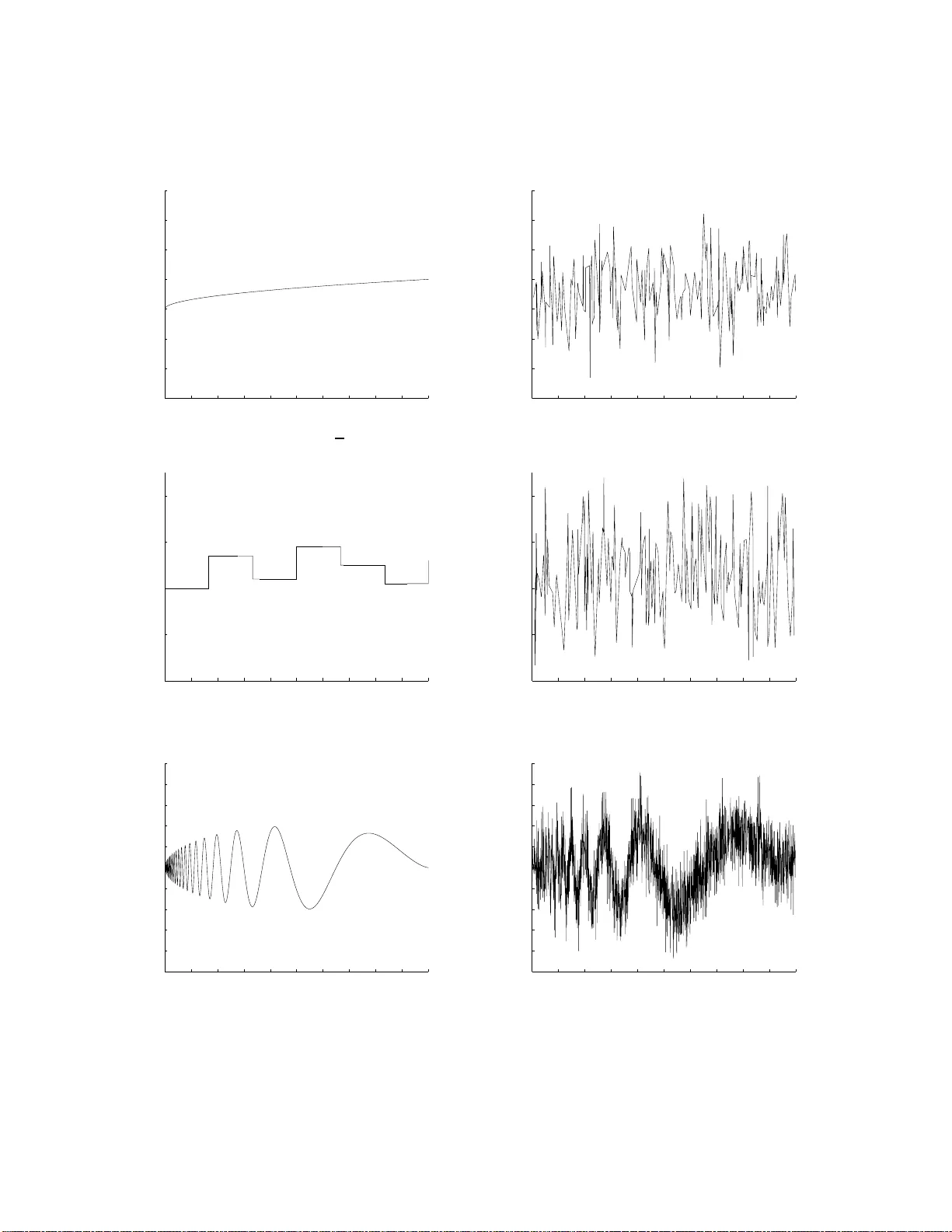
Submitte d to the Annals of Statistics arXiv: 0802. 0566 V -F OLD CR OSS-V ALID A TION IMPR O VED: V -F OLD PENALIZA TION By Syl v ain Arlot Universit´ e Pa ris-Sud W e stud y the eﬃciency of V -fold cross-v a lidation (V F CV) for model selection from the non-asymptotic v iewpoint, and suggest an impro vemen t on it, whic h we call “ V -fold p enalization”. Considering a particular (though simple) regression problem, w e pro ve that V FC V with a boun ded V is sub optimal for model selec- tion, b ecause it “o ve rp enalizes” all the more that V is large. H ence, asymptotic optima lit y requires V to go to inﬁnity . Ho w ever, when the signal-to-noise ratio is lo w, it appears that o ver p enalizing is n ec- essary , so that the optimal V i s not alw a ys the larger one, despite of the v aria bilit y issue. This is conﬁrmed by some sim ulated data. In order to improv e on the prediction p erformance of VFC V, we deﬁne a n ew mo del selection procedure, called “ V -fol d p enalization” (p enVF). It is a V -fold subsampling version of Efron’s b o otstrap p enalties, so that i t has the same computational cost as VFCV, while b eing more ﬂexible. In a heteroscedastic regression framew or k, a ssum- ing the mo dels to hav e a particular structu re, we prov e that p enVF satisﬁes a non-asympt otic oracle inequality with a leading constan t that tend s to 1 when the sample size go es to inﬁnity . In particular, this implies adaptivit y to the smooth ness of the regression function, even w ith a highly h eteroscedastic noise. Moreov er, it is easy to o ver- p enalize with p enVF, ind epen dently from the V parameter. A simu- lation study sho ws that this results in a signiﬁcan t impro vemen t on VFC V in non-asympt otic situations. 1. In tro duction. There are typica lly t w o kinds of mo del selection criteria. On the one- hand, p enalized criteria are the sum of an empirical loss an d some p enalt y term, often measurin g the complexit y of the mo dels. This is the case of AIC (Ak ai k e [Ak a7 3]), Mallo ws’ C p or C L (Mallo w s [Mal73]) and BIC (Sc h w arz [Sch78]), to name but a few. On the other hand, cross- v alidation (Allen [All74 ], Stone [Sto74], Geisser [Gei75]) and related criteria are b ased on the idea of d ata splitting. Part of the d ata (the training set) is used for ﬁtting eac h mo del, and the rest of the data (the v alidati on s et) is used to measure the p erformance of the mo dels. T here are sev eral versions of cross-v alidat ion (CV), e.g. lea v e-o ne-out (LOO, also called ordinary CV), AMS 2000 subje ct classiﬁc ations: Primary 62G09; secondary 62G08 , 62M20 Keywor ds and phr as es: non-parametric sta tistics, sta tistical l earning, resampling, non-asymptotic, V -fold cross- v ali dation, mod el selection, p enalization, non-p arametric regressio n, adaptivity, heteroscedastic data 1 2 ARLOT, S. lea v e- p -out (LPO, also called d elete- p CV) and generalized CV (Cra ven and W ah ba [CW79]). In practical applications, cross-v alidation is often computational ly very exp ensive . This is why less greedy C V algorithms hav e b een prop osed, among which V -fold cross-v alidation (VFCV, Geisser [Gei 75]) and rep eated learning testing metho d s (Breima n et al. [BF O S84]). In this article, w e mainly consider VF CV — which seems to b e the most widely used no w ada ys — when the goal of mo d el selection is to b e eﬃci e nt , i.e. to minimize the p r ediction risk among a family of estimators. Let us emphasize that this is quite diﬀeren t from pic kin g up the “true mo d el”, whic h is often recalle d as the identiﬁc ation or c onsistency issu e. The prop erties of CV (in particular lea ve- p -out) for prediction and mo del iden tiﬁcation ha ve b een widely stud ied from the asymptotical viewp oin t. It t ypically dep ends on the s p litting ratio, i.e. the ratio b et ween the sizes of the v alidation and training sets ( p/ ( n − p ) in the lea ve- p -o ut case; 1 / ( V − 1) for V -fold cross-v alidation). Th is has b een s h o wn for instance b y S h ao [S ha97] (for regression on linear mo dels) and by v an d er Laan, Dudoit and Keles [vdLDK04] (for densit y estimatio n). Asymptotic optimalit y o ccurs when this ratio go es to zero at inﬁn it y , as shown b y Li [Li87] for th e lea v e-one-out, and generalized by Sh ao [Sha97] for the lea ve- p -out with p ≪ n , b oth in the regression setting, when all th e mo dels are linear. Other asymptotic results ab out CV in regression can b e found in the b o ok by Gy¨ orﬁ et al. [GKKW02], and in the p ap er of v an d er Laan, Dudoit and Keles [vd LDK04] f or densit y estimation. Notice that the b eha viour of these p ro cedures changes completely when the goal is consistency; w e r efer to Y ang [Y an07] and Sect. 5.4 b elo w for references on this p roblem. When it comes to p ractical application, a ma jor qu estion is ho w to c ho ose the tu n ing pa- rameters of CV pro cedures, since their p erformance strongly dep end on them. In the case of VF CV, this means choosing V . Basicall y , there are three comp eting factors. First, the VFCV estimator of the prediction error, crit VFCV , is biased, and its bias decreases with V . As sho wn by Burman [Bur89, Bur90], it is p ossible to correct this bias; otherwise, V sh ould not b e tak en to o small. Second, the v ariance of crit VFCV dep ends on V : it is alw a ys decreasing for small v alues of V , b ut then it can either sta y decreasing (as in the linear regression case [Bur89]) or start to increase b efore V = n (as in some classiﬁcation pr oblems [Bre96, HTF01, MSP 05 ] or in densit y estimatio n [CR08]; see Sect. 2.3). Third, the computational cost of VFCV is prop ortional to V , so that the theoretic optimum (taking only b ias and v ariabilit y into accoun t) can not alw a ys b e computed. More pr ecisely , it is n ecessary to understand we ll ho w the p erformance of VF CV dep ends on V b efore taking into accoun t the computational cost. T h is is one of the p urp oses of this article . W e h ere aim at providing a b etter un derstanding of some CV p ro cedures (including VFCV) from the non-asymptotic viewp oint . This ma y ha v e t w o m a jor implications. First, non-asymptotic results are made to h an d le collectio ns of mo dels whic h ma y dep end on the sample size n : their sizes ma y t ypically b e a p o wer of n , and they ma y con tain mo d els whose complexities gro w with n . Such collectio ns of mo d els are particularly signiﬁcan t for designing adaptiv e estimators of a function wh ich is only assumed to b elong to some h¨ olderian ball, wh ic h may r equire an V - FOLD PENALIZA TION 3 arbitrarily large num b er of parameters. Second, in several practical app licatio ns, we are in a “non-asymptotic situation” in the sense that the signal-to -noise ratio is lo w. W e shall see in the follo wing that it s h ould really b e tak en into accoun t for an optimal tu n ing of V . It is w orth noticing that suc h a non-asymptotic app roac h is not common in the literature, sin ce most of the results already men tioned are asymp totic, and none is considering our second p oin t ab ov e. Another imp ortan t p oin t in our approac h is that our fr amew ork includes sev eral kin ds of heteroscedastic data. W e only assume that the observ ations ( X i , Y i ) 1 ≤ i ≤ n are i.i.d. with Y i = s ( X i ) + σ ( X i ) ǫ i , where s : X 7→ R is the (unkno w n) regression function, σ : X 7→ R is the (un kno wn) noise-lev el, and ǫ i has a zero m ean and a unit v ariance conditionally to X i . In p articular, the noise-lev el σ ( X ) can b e strongly dep end en t from X , and the d istribution of ǫ can itself dep end from X . Suc h d ata are generally considered as very diﬃcult to handle, b ecause w e ha v e no inform ation on σ , making ir regularities of the s ignal h arder to distinguish from noise. Then, s imple m o del selectio n pro cedures suc h as Mallo ws’ C p ma y not w ork (see Chap. 4 of [Arl07] for a theoretical argumen t), and it is natural to hop e th at VF C V or other resampling metho ds ma y b e robust to heteroscedastic it y . In this article, b oth theoretical and sim u lation results conﬁrm this fact. In Sect. 2, w e pro vide a non-asymptotic analysis of the p erformance of VF C V. The aforemen- tioned b ias turns out in to a non-asymptotic negativ e result (Thm. 1), sho wing a rather simp le problem for wh ic h VF CV can not satisfy an oracle inequalit y with leading constan t smaller than κ ( V ) − ǫ n , with κ ( V ) > 1 for an y V ≥ 2 and ǫ n → 0. In p articular, VF CV with a b ounded V can n ot b e asymptotical ly optimal. But our analysis also has a ma jor p ositiv e consequence in some “non-asymptotic” situations. Indeed, by considerin g VF CV as a p enalizatio n pro cedure, our previous result can b e in terpr etated as an ov erp enalization pr op ert y of VF CV. Th is should b e related to the fact that the eﬃciency of p enalizatio n m etho d s (like Mallo ws’ C p ) is often impro v ed by o verpenalization, when the signal-to-noise ratio is small. Then, one can exp ect the optimal V for VF CV to b e smaller than n , ev en for least- squares regression, wh ic h is conﬁr med b y the sim u lation study of Sect. 4. So, it app ears that c ho osing the optimal V for VF CV ma y b e quite hard. In addition, the optimal c hoice ma y not b e satisfactory when it corresp onds to a highly v ariable criterion such as the 2-fold CV one. It is lik ely that there is some ro om left here to impro ve on VFCV. This is wh y we prop ose in S ect. 3 another V -fold algorithm, that w e call “ V -fold p enalizati on” (p enVF). It is based up on Efron’s resampling heuristics [Efr79], in the same wa y as Efron’s b o otstrap p enalt y [Efr83], bu t with a V -fold subsamp ling scheme instead of the b o otstrap. It th u s has exactly the same computational cost as the classical VF CV, and our results show that is has a similar robustness prop ert y , in some heteroscedastic regression framework. In addition, it turns out to b e a generaliz ation of Burman’s corrected VF CV [Bur89, Bur90] (at least when the splitting in to V blo cks is r egular). T he main adv ance of p enVF b eing that it is straigh tforw ard 4 ARLOT, S. to o v erp enalize within an y factor w hen this is required, for instance w h en the signal-to-noise ratio seems lo w. In the least-square r egression framew ork, when w e hav e to select among histogram mo d els (see Sect. 2.2 for an accurate deﬁnition), w e pr ov e that p enVF satisﬁes a non-asymptotic oracle inequalit y with a leading constan t almost one (Thm. 2). T o our knowledge , suc h a non-asymptotic result is new for any V -fold mo del selection pro cedure. One of its stren gths is that it requires v ery few assumptions on the noise, allo wing in particular heteroscedasti cit y . It is a strong result for p enVF — which w as not bu ilt for this particular setting at all — to improv e on VF CV for suc h diﬃcult pr oblems, where VF C V is among the b est pr o cedures o verall. As a consequence of Thm. 2, one can use p enVF with the family of regular histograms in order to obtain an estimator adaptiv e to the sm o othness of the regression fun ction, when the noise is heteroscedastic (wh ile ha vin g no information at all on the distribution of the noise). Notice that we only consider this result as a ﬁr st step tow ards a more general theorem, without the restriction to histograms, as discussed in Sect. 5.3. The main interest of this to y f ramew ork is that w e can study it deeply , and then deriv e general heu r istics for pr actical use. As an illustration to our theoretical study , we pr o vide the results of a simulat ion study in Sect. 4. It conﬁrms the go o d p erformances of p enVF against b oth VFCV and th e simpler Mal- lo ws’ C p criterion, in particular for diﬃcult heteroscedastic p r oblems. W e also show ho w u seful ma y b e the ﬂexibilit y of p enVF wh en th e signal-to-noi se ratio is lo w. By decoupling V from the o verpenalization factor, w e allo wed a signiﬁcan t impro vemen t of the p erformance of b oth VF C V and its b ias-correcte d version. Finally , our results are d iscussed in Sect. 5. Th e remaining of the pap er is d ev oted to some probabilistic to ols (App . A) and pro ofs (App . B). 2. P erformance of V -fold cross-v alidat ion. In this sec tion, w e pro vide a n on-asymptotic study of V -fold cross-v alidation (VF CV) in the least-squares regression fr amew ork. In order to mak e explicit computations p ossible, w e fo cus on the case where eac h mo del is an “histogram mo del”, i.e. th e v ector space of piece wise constant functions on so me ﬁxed partition of th e feature space. This is only a ﬁrst th eoretical step. W e us e it to deriv e heuristics, that should help the p ractical user of VFCV in any f ramew ork. Notice also that we do not assume that the regression function itself is p iecewise constan t. 2.1. Gener al fr amework. First consider the general p rediction setting: X × Y is a measurable space, P an unkno w n probabilit y mea sure on it and w e observ e some data ( X 1 , Y 1 ) , . . . , ( X n , Y n ) ∈ X × Y o f common la w P . Let S b e the set of predictors (measurable f unctions X 7→ Y ) and γ : S × ( X × Y ) 7→ R a con trast fu nction. Giv en a family ( b s m ) m ∈M n of data-dep endent predic- tors, our goal is to ﬁnd the one minimizing the prediction loss P γ ( t ) := E ( X,Y ) ∼ P [ γ ( t, ( X, Y ))]. Notice that the exp ectation h ere is only tak en w.r.t. ( X , Y ), so that P γ ( t ) is random when t is random ( e.g. data-driv en). Assuming that there exists a minimizer s ∈ S of the loss (the Ba y es predictor), w e will often consider the excess loss l ( s, t ) = P γ ( t ) − P γ ( s ) ≥ 0 instead of the loss. V - FOLD PENALIZA TION 5 W e assume that eac h predictor b s m can b e writte n as a function b s m ( P n ) of the empirical distribution of the data P n = n − 1 P n i =1 δ ( X i ,Y i ) . The case-example of such a pred ictor is the empirical r isk minimizer b s m ∈ arg min t ∈ S m { P n γ ( t ) } , wh ere S m is an y set of p redictors (called a mo del ). In the classical versio n of VFCV, we ﬁrst choose some partition ( B j ) 1 ≤ j ≤ V of the indexes { 1 , . . . , n } . Then , we d eﬁ n e P ( j ) n = 1 Card( B j ) X i ∈ B j δ ( X i ,Y i ) b s ( j ) m = b s m  P ( j ) n  P ( − j ) n = 1 n − Card( B j ) X i / ∈ B j δ ( X i ,Y i ) b s ( − j ) m = b s m  P ( − j ) n  . The ﬁnal VF CV estimator is b s b m VFC V ( P n ) with (1) b m VFCV ∈ arg min m ∈M n { crit VFCV ( m ) } and crit VFCV ( m ) := 1 V V X j =1 P ( j ) n γ  b s ( − j ) m  . It is classica l to assu m e that the partition ( B j ) 1 ≤ j ≤ V is regular, i.e. that ∀ j , | Card( B j ) − n/V | < 1. In order to u nderstand deeply the prop erties of VF CV, w e ha v e to compare precisel y crit VFCV ( m ) to the excess loss l ( s, b s m ). A crucial p oin t is to compare th eir exp ectati ons, wh ic h is qu ite hard in general. This is why we restrict ourselve s to a particular fr amew ork, n amely the histogram regression one. W e describ e it in the next su bsection. 2.2. The histo gr am r e gr ession c ase. In the regression fr amew ork, the d ata ( X i , Y i ) ∈ X × R are i.i.d. of common la w P . Denoting by s the regression fu n ction, we h av e (2) Y i = s ( X i ) + σ ( X i ) ǫ i where σ : X 7→ R is the h eteroscedastic noise-lev el and ǫ i are i.i.d. cen tered noise terms, p ossibly dep endent from X i , but with mean 0 and v ariance 1 conditionally to X i . In order to simplify the th eory , w e will make t wo main assu mptions on the d ata throughout this pap er: σ ( X ) ≥ σ min > 0 a.s. and k Y k ∞ ≤ A < + ∞ . Notice that we do not assum e σ min and A to b e kno wn from the statistician. Moreo ver, those t wo assumptions can b e relaxed, as sho w n b y Ch ap . 6 and Sect. 8.3 of [Arl07]. T he feature sp ace X is t ypically a compact subs et of R d . W e u s e the least-squares con trast γ : ( t, ( x, y )) 7→ ( t ( x ) − y ) 2 to measure the qu alit y of a predictor t : X 7→ Y . As a consequence, the Ba ye s predictor is the regression fu n ction s , and the excess loss is l ( s, t ) = E ( X,Y ) ∼ P ( t ( X ) − s ( X )) 2 . T o eac h mo del S m , w e asso ciate the empiric al risk minimizer b s m := b s m ( P n ) = arg min t ∈ S m { P n γ ( t ) } 6 ARLOT, S. (when it exists and is unique). Deﬁne also s m := arg min t ∈ S m P γ ( t ). W e n ow fo cus on histograms. Eac h m o del i n ( S m ) m ∈M n is the set of piecewise co nstan t functions (histograms) on some partition ( I λ ) λ ∈ Λ m of X . It is thus a v ector s pace of d imension D m = Card(Λ m ), spanned by the family ( 1 I λ ) λ ∈ Λ m . As this b asis is orthogonal in L 2 ( µ ) for any probabilit y measure µ on X , we can mak e explicit compu tations. T h e follo wing notations will b e useful throughout this article. p λ := P ( X ∈ I λ ) b p λ := P n ( X ∈ I λ ) σ 2 λ := E h ( Y − s ( X ) ) 2    X ∈ I λ i . Remark that b s m is uniquely deﬁ n ed if and only if eac h I λ con tains at least one of the X i , i. e. min λ ∈ Λ m { b p λ } > 0. Prop. 1 b elo w compares the V -fold criterion and the ideal criterion P γ ( b s m ) in exp ectation. Pr oposition 1 . L et S m b e the mo del of histo gr ams asso ciate d with the p artition ( I λ ) λ ∈ Λ m and ( B j ) 1 ≤ j ≤ V some “almost r e gu lar” p artition of { 1 , . . . , n } , i.e. such that max j  Card( B j ) n  ≤ c B < 1 and sup j      Card( B j ) n − 1 V      ≤ ǫ r eg n − − − → n →∞ 0 . Then, the e xp e ctation of the ide al and V -fold criteria ar e r esp e ctive ly e qual to E [ P γ ( b s m ) ] = P γ ( s m ) + 1 n X λ ∈ Λ m ( 1 + δ n,p λ ) σ 2 λ (3) E [ crit VFCV ( m ) ] = P γ ( s m ) + V V − 1 × 1 n X λ ∈ Λ m  1 + δ ( V F ) n,p λ  σ 2 λ (4) wher e δ n,p only dep ends on ( n, p ) , δ ( V F ) n,p dep ends on ( n, p ) and the p artition ( B j ) 1 ≤ j ≤ V , but b oth ar e smal l when the pr o duct np is lar ge: | δ n,p | ≤ L 1 and    δ ( V F ) n,p    ≤ L 2 h ǫ r eg n + max  ( np ) − 1 / 4 , e − np (1 − c B )  i , wher e L 1 is a numeric al c onstant ant L 2 only dep ends on c B . Remark 1 . Since w e deal with histograms, b s m is not d eﬁ n ed when min λ ∈ Λ m b p λ = 0, whic h o ccurs w ith p ositiv e probabilit y . W e then h av e to tak e a con ve n tion for P γ ( b s m ) (on the ev en t min λ ∈ Λ m { b p λ } = 0, whic h has generally a very small probabilit y) so that it has a ﬁnite exp ecta- tion. The same kind of problem o ccur with crit VFCV . See the pro of of Prop. 1. Prop. 1 is consisten t with Burman’s asymptotic estimate of the b ias of VFCV [Bur89]. Th e ma jor adv ance here is that it is non-asymptotic, and w e hav e explicit u pp er b ounds on the V - FOLD PENALIZA TION 7 remainder terms (see the pro of of Prop. 1 in App. B.4). It sho ws that the classical V -fold cross- v alidation o v erestimates the v ariance term n − 1 P λ ∈ Λ m σ 2 λ , b ecause it estimates the generalization abilit y of b s ( − j ) m , which is built up on less data than b s m . This in terpretation is consisten t with the results of Shao [Sha97] on linear regression, and v an der Laan, Dudoit and Keles [vdLDK04] in the d ensit y estimatio n framew ork. When V sta ys b ounded as n gro w s t o inﬁnity , it is then natural to think that VF CV is underﬁtting, and th u s b e sub optimal for pred iction. Since Prop. 1 is non-asymptotic and quite accurate, w e are no w in p osition to pro v e su c h a resu lt. Theorem 1 . L et n ∈ N , ( X i , Y i ) 1 ≤ i ≤ n b e i.i .d. r andom variables, with X ∼ U ([0 , 1]) and Y = X + σ ǫ with σ > 0 , E [ ǫ | X ] = 0 , E  ǫ 2   X  = 1 and k ǫ k ∞ < + ∞ . L et M n = { 1 , . . . , n } and ∀ m ∈ M n , S m b e the mo del of r e gular histo gr ams with D m = m p ie c es on X = [0 , 1] . L e t V ∈ { 2 , . . . , n } and ( B j ) 1 ≤ j ≤ V b e some p artition of { 1 , . . . , n } such that for every j ,   Card( B j ) − nV − 1   < 1 . Then, ther e is an event of pr ob ability at le ast 1 − K 1 n − 2 on which (5) l ( s, b s b m VFC V ) ≥ (1 + κ ( V ) − ln( n ) − 1 / 5 ) inf m ∈M n { l ( s, b s m ) } , for some c onstant κ ( V ) > 0 dep ending only on V (and de c r e asing as a function of V ), and a c onstant K 1 which dep ends on σ , A and V . W e no w make a few commen ts: • In the same framewo rk, usin g similar arguments, w e can pro ve an up p er b oun d on l ( s, b s b m VFC V ) sho w ing that the constan t 1 + κ ( V ) is exact (up to the ln( n ) − 1 / 5 term). In p articular, l ( s, b s b m VFC V ) inf m ∈M n { l ( s, b s m ) } a.s. − − − − − → n → + ∞ 1 + κ ( V ) = 1 + 2 2 / 3 3 " 1 −  V − 1 V  1 / 3 # 2 > 1 . • When ( B j ) 1 ≤ j ≤ V is not assumed reg ular, the proof of Prop. 1 sho ws that the fac tor V / ( V − 1) b ecomes P V j =1 n/ ( n − Card( B j )) whic h is alw a ys larger, b ecause x 7→ ( n − x ) − 1 is conv ex. On the other hand , if one c h o oses a ( X i ) 1 ≤ i ≤ n -dep endent partition suc h that for ev ery λ ∈ Λ m , C ard { X i ∈ I λ and i ∈ B j } is (almost) indep end en t from j , th en a similar pro of sh o ws that δ ( V F ) n,p is made m uc h s maller than the pr evious upp er b ound . In a n utshell, it seems that the b est p erformance of VF CV corresp onds in general to the regular partition case, for whic h (5 ) holds. • Although w e restrict in Thm. 1 to a ve ry particular problem, a similar resu lt sta ys v alid m u c h more generally , p ossib ly with a diﬀeren t v alue for the constant κ ( V ). Th e only purp ose of our a ssumptions is to c ompare v ery precisely crit VFCV ( m ) and P γ ( b s m ) as functions of m . Since D b m VFC V is sm aller than the optim um from a m ultiplicativ e factor indep end ent from n only , this analysis strongly dep ends on h o w P γ ( b s m ) v aries with m . 8 ARLOT, S. • One can easily extend this r esult to any cross-v alidation lik e metho d, when t w o conditions are satisﬁed. First, the ratio b et w een the size of the training set and n has to b e upp er- b ound ed by 1 − V − 1 < 1 (uniformly in n ). S econd, the num b er of training sets considered has to b e b ound ed by B max (from wh ic h K 1 ma y d ep end). Th is includes for instance the hold-out case, and rep eated learning-testing metho ds. Notice that the second assump tion is mainly tec hnical; if w e w ere able to pro ve the corresp onding concen tration inequalities, the lea ve - p -out w ith p ∼ n/V sh ould h av e appr o ximately the same prop erties. 2.3. How to cho ose V . 2.3.1. Classic al analysis. There are thr ee wel l-kno wn factors to tak e into accoun t in order to c ho ose V : • bias : when V is to o small, crit VFCV o verest imates the v ariance term in P γ ( b s m ), which leads to underﬁtting and sub optimal mo del selecti on (Th m. 1). • variability : the v ariance of crit VFCV ( m ) is a decreasing function of V , at least in the linear regression framework (see Burman [Bur89] f or an asymptotic expans ion of this v ariance). In general, V = 2 is kno wn to b e quite v ariable b ecause of the single split. When the prediction algorithm ( X i , Y i ) 1 ≤ i ≤ n 7→ b s m is un stable ( e.g. classiﬁcation with CAR T, as noticed by Hastie, Tibshirani and F riedman [HTF01]; see also Breiman [Bre96]), the lea ve- one-out criterion ( i.e. V = n ) is also known to b e quite v ariable, bu t this phenomenon seems to disapp ear when b s m is more stable (Molinaro, Simon and Pfeiﬀer [MSP05]). In particular, in the least-squares regression framewo rk, the v ariance of crit VFCV ( m ) should decrease with V . • c omputational c omplexity : V -fold cross-v alidation needs to compute at least V empirical risk minimizers for eac h mo del. In the least-squares regression setting, V h as to b e c h osen large in order to improv e accuracy (b y reducing bias and v ariabilit y); on the con trary , computational issues arise wh en V is too big. This is why V = 5 and V = 10 are ve ry classical and p opu lar c hoices. 2.3.2. The non-asymptotic ne e d for overp enalization. W e now come to some particularit y of the non-asymptotic viewp oint. Indeed, our pr o of of Thm. 1 sho ws that the asymptotic b ehavio ur of h old-out and cross-v alidation criterions only d ep end on their bias, b ecause all these criterions are suﬃcien tly close to th eir exp ectations asymp totically . How ev er, this is not true w hen the sample size is ﬁxed, and even the less v ariable criterions are far from b eing deterministic. As a consequence, using an unbiase d estimator is no longer a guaran tee of b eing optimal, since it can still lead to choosing a very p o or mo d el w ith a p ositiv e probabilit y . In order to analyze this phen omenon, it is useful to tak e the p enalization viewp oin t. T h e idea of p enalizatio n for mo del select ion is to d eﬁne (6) b m ∈ arg min m ∈M n { P n γ ( b s m ) + p en( m ) } , V - FOLD PENALIZA TION 9 0 1 2 3 1 2 3 4 5 6 7 8 Overpenalization constant E[Loss(estimator)]/E[Loss(oracle)] Fig 1 . The non-asymptotic ne e d f or overp enalization: the pr e diction p erformanc e C or (deﬁne d in Se ct. 4.1) of the mo del sele ction pr o c e dur e (6) with p en( m ) = C o v E [ pen id ( m ) ] is r epr esente d as a function of C o v . Data and mo dels ar e the ones of exp eriment (S1): n = 200 , σ ≡ 1 , s ( x ) = sin( π x ) . Se e Se ct. 4 for mor e details. where p en( m ) is c hosen so that P n γ ( b s m ) + p en( m ) is close to the p rediction error P γ ( b s m ). In other words, the “ideal p enalt y” is (7) p en id ( m ) := ( P − P n ) γ ( b s m ) . According to Prop. 1 and (38) (wh ich follo ws its pro of ), in the histogram r egression case, w e can compu te the exp ectation of the ideal p enalt y: (8) E [ p en id ( m ) ] = 1 n X λ ∈ Λ m ( 2 + δ n,p λ ) σ 2 λ , whic h is close to Mallo w s ’ C p p enalt y 2 σ 2 D m n − 1 in the homoscedastic case. T he p oint is that o verpenalization (that is, taking p en larger than p en id , ev en in exp ectation) can impr o ve the prediction p erformance of b s b m when the signal-to-noise ratio is small. This can b e seen on Fig. 1, according to whic h the optimal ov erp enalization constan t C ⋆ o v seems to b e b et ween 1 . 2 and 1 . 7 for this p articular mo d el selection problem. See also [Arl07] for a longer d iscussion of this problem. 2.3.3. Cho osing V in the non-asympto tic fr amework. Sin ce V -fold cross-v alidation is choosing the m o del b m VFCV whic h m inimizes some criterion crit VFCV , it can b e written as a p enalization pro cedure: it satisﬁes (6) with p en VFCV ( m ) := crit VFCV ( m ) − P n γ ( b s m ) . 10 ARLOT, S. Using again Prop. 1 and (38 ), w e can compu te its exp ectatio n: E [ p en VFCV ( m ) ] = 1 n X λ ∈ Λ m  1 + V V − 1  1 + δ ( V F ) n,p λ   σ 2 λ . Compared to (8), this sh o ws that V -fold cross-v alidation is o ve rp enalizing within a factor 1 + 1 / (2( V − 1)). W e can no w revisit the question of c ho osing V for optimal prediction, in suc h a non-asymptotic situation: • the overp enalization factor is 1 + 1 / (2( V − 1)). • the varianc e of crit VFCV roughly decreases with V . • the c omputational c omplexity of computing crit VFCV is roughly prop ortional to V . First, tak e o nly the prediction p erformance into accoun t. Th e v ariabilit y question should b e less cru cial than o v erp enalizatio n, b ecause the v ariance of crit VFCV dep ends only on V through second order terms, according to the asymptotic computations of Burman [Bur 89 ]. Since the optimal o v erp enalization constan t is C ⋆ o v > 1, the p erformance of V -fold cross-v alidation should b e optimal for some V ⋆ < n . This analysis is conﬁr med by the simula tion study of S ect. 4, w here V = 2 p ro vid es b etter p erform ance than V = 5 and V = 10 for seve ral diﬀerent exp erimen ts. No w, if computational cost comes into the balance, or if we consider less stable prediction algorithms than least-squares regression estimators, th e optimal V ma y b e ev en smaller. What- ev er the fr amew ork, it seems quite diﬃcult to ﬁnd the optimal V , even if C ⋆ o v w as known (whic h is far fr om b eing the case in general). It would b e at least necessary to und erstand well ho w the v ariance of crit VFCV dep ends on V in the non-asymptotic fr amew ork. This is a diﬃcult pr actica l problem, since “there is no u n iv ersal (v alid und er all distributions) unbiased estimator of the v ariance of V -fold cross-v alidation” (Bengio and Grandv alet [BG04]). In th e d ensit y estimatio n framew ork, this question has b een tac kled recent ly by Celisse and Robin [CR08]. The conclusion of th is section is that c h o osing V for V -fold is a v ery complex issue in practice, ev en indep end en tly fr om the cost of compu ting crit VFCV . Moreo ver, it seems u nsatisfactory to select a mo del according to a criterion as v ariable as the 2-fold cross-v alidation one wh en V ⋆ = 2 b ecause of the need for o v erp enalization. Finally , wh en the signal-to -noise r atio is large, we w ould lik e to obtain a nearly unbiased p ro cedure without ha vin g to tak e V very large, w hic h can b e computationally too h ea vy . In other words, w e w ould like to decouple the c hoice of an o v erp enalizatio n factor from the v ariabilit y issue (wh ic h is essent ially linked with complexit y). Th e dr awbac k of V -fol d cross- v alidation is that they b oth dep end on the V parameter. As we shall see in the next section, suc h a decoupling can b e naturally obtained through the u se of p enalization. 3. An alt ernativ e V -fold algorithm: V -fold p enalties. There are seve ral wa ys to de- ﬁne V -fold cross-v alidation like p enalization pro cedures with a tun able o verpenalization factor, V - FOLD PENALIZA TION 11 indep end ent from the V p arameter. A ﬁr st idea ma y b e to multiply p en VFCV ( m ) by a constan t i.e. to use (6) with the p enalt y p en( m ) = C o v  1 + 1 2( V − 1)  − 1 ( crit VFCV ( m ) − P n γ ( b s m ) ) . F rom the pr o of of Thm. 1 (see also the one of Th m. 2 b elo w), it is clear that when C o v ∼ 1, this pro cedu re satisﬁes with large p robabilit y a non-asymptotic oracle inequalit y with leading constan t 1 + ǫ n , and more generally an oracle inequalit y with leading constan t K ( C o v ) ≥ 1. Ho wev er, th is may s eem a little artiﬁcial, and strongly dep endent from the h istogram r egression framew ork in wh ic h the compu tations of Pr op. 1 work. In this section, w e consider another approac h, that we call “ V -fold p enalization”, whic h seems more natural to us. W e shall see b elo w that it is closely related to an idea of Burman [Bur89, Bur90] for correcting the bias of V -fold cross-v alidation. Ho wev er, Burman did not consider his metho d as a p enalization one. His goal w as only to obtain an un b iased estimate of th e pr ediction error, so th at it is not straigh tforward to choose an ov erp enalizatio n factor d iﬀeren t fr om 1 with his metho d. This is a ma jor diﬀerence with our approac h. 3.1. Deﬁnition of V -fold p enalties. 3.1.1. Gener al fr amework. W e come bac k to the general setting of Sec t. 2.1. Recall t hat eac h p r edictor b s m can b e written as a fu nction b s m ( P n ) of the empirical distribu tion of the data P n = n − 1 P n i =1 δ ( X i ,Y i ) . W e wa n t to b uild a p enalizatio n metho d , i.e. c h o ose b m according to (6), so that the prediction err or of b s b m is as small as p ossible. T his could b e done exactly if w e knew the ideal p enalt y p en id ( m ) = ( P − P n ) γ ( b s m ( P n )), b ut this qu an tity dep ends on the unknown distribution P . F ollo wing a heu r istics d ue to Efron [Efr 79], w e prop ose to deﬁne p en as the resampling estimate of p en id , according to a V -fold sub sampling sc heme. W e ﬁrst recall the general form of this h euristics. Basicall y , the r esampling heuristics tells that one can mimic the relationship b et ween P and P n b y bu ilding a n -sample of common distribu tion P n (the “resample”). P W n denoting the em- pirical distribution of the r esample, the pair ( P , P n ) should b e close (in distribution) to the pair ( P n , P W n ) (conditionally to P n for the latter distribution). Th en, the exp ectati on of any quantit y of the form F ( P , P n ) can b e estimated by E W h F ( P n , P W n ) i , wh ere E W [ · ] denotes exp ectation w.r.t. the resampling randomness. In the case of p en id , this leads to Efron’s b o otstrap p enalt y [Efr83]. Later on, this heuristics has b een generalized to other resampling sc hemes, with the ex- c hangeable wei gh ted b o otstrap (Mason and Newton [MN92], Præstgaard and W ellner [PW93]). The empirical distribution of the resample then h as th e general form P W n := 1 n n X i =1 W i δ ( X i ,Y i ) with W ∈ R n an exc h angeable w eight v ector, indep end ent from the data ( W is sa id to be excha nge able wh en its d istribution is inv arian t b y any p erm u tation of its co ordinates). F romont [F ro07] used it successfully (with a p articular 12 ARLOT, S. upp er b ound on p en id ) to build global p enalties in the classiﬁcation framew ork. Exchangea ble resampling p enalties (generalizi ng Ef r on’s b o otstrap p enalt y) ha ve also b een recent ly prop osed, and stu d ied in the regression fr amew ork [Arl07]. The idea of V -fold p enalties is to use a V -fol d subsampling scheme instead, i.e. tak e W i = V V − 1 1 i / ∈ B J with J ∼ U ( { 1 , . . . , V } ) in dep endent from the data ( U ( E ) denotes the uniform distribution o ver the set E ). Then, P W n = P ( − J ) n and w e obtain the follo wing algorithm. Algorithm 1 ( V -fol d p enalizati on) . 1. Cho ose a partition ( B j ) 1 ≤ j ≤ V of { 1 , . . . , n } , as regular as p ossible. 2. Cho ose a constan t C ≥ C W, ∞ = V − 1. 3. Compute th e follo wing resampling p enalt y for eac h m ∈ M n : p en( m ) = p en VF ( m ) := C V V X j =1 h P n γ  b s m  P ( − j ) n   − P ( − j ) n γ  b s m  P ( − j ) n   i . 4. Cho ose b m according to (6). Remark 2 (Ab out the constant C ) . Contrary to Efron’s r esampling heur istics, w e hav e to put a constan t C 6 = 1 in fron t of the p enalt y (p en b eing an un biased estimator of p en id when C = C W, ∞ ). This is b ecause eac h W i has a v ariance ( V − 1) − 1 6 = 1 (we only normalized W s o that E [ W i ] = 1 for ev ery i ). According to Lemma 8.4 of [Arl07 ], the right normalizing constan t can b e deriv ed from the exc hangeable case. As a consequence, from Theorem 3.6.13 in [vdVW96], C W, ∞ ∼ n →∞ n − 1 n X i =1 E ( W i − 1 ) 2 ! − 1 ∼ n →∞ V − 1 . The asymptotic v alue of C W, ∞ can also b e deriv ed from the computations of Burman [Bur89] in the linear r egression framework. I ndeed, with our notations, Bu r man’s criterion (formula (2.3) in [Bur89]) is crit corr . VF ( m ) := crit VFCV ( m ) + P n γ ( b s m ) − 1 V V X j =1 P n γ  b s ( − j ) m  = P n γ ( b s m ) + 1 V V X j =1 h  P ( j ) n − P n  γ  b s ( − j ) m  i . If all the blo cks of the partition ha ve the same size n/V , then P ( j ) n − P n = ( V − 1)( P n − P ( − j ) n ), s o that Burman’s corrected VF CV coincides exactl y with V -fold p enalizati on when C = V − 1. Since crit corr . VF ( m ) is an asymptotical ly unbiase d estimato r of P γ ( b s m ) (at least for linear regression), the result follo ws. F rom the non-asymp totic viewp oin t, we prov e in Sect. 3.2 b elo w that V − 1 also leads to an u n biased estimator of p en id in the h istogram regression case. V - FOLD PENALIZA TION 13 Notice also that w e do not assu me that C = C W, ∞ , but only C ≥ C W, ∞ . This is a ma jor qualit y of V -fold p enalizatio n (penVF): it is straigh tforw ard to c h o ose any o verpenalization factor, indep endently from V . F urther comments ab out the c hoice of C and V are made in Sect. 5. 3.1.2. The histo g r am r e gr ession c ase. W e no w come b ac k to the framew ork of S ect. 2.2, in whic h w e can analyze deep er Algorithm 1. Remind that histograms are not our ﬁn al goal, but only a con v enient setting from which we can deriv e heuristics for practical us e of p enVF in an y framew ork. F rom no w on, ( S m ) m ∈M n is a collectio n of histogram mo dels and ( b s m ) m ∈M n the asso ciated collect ion of least- squares estimators. W e ﬁrst int ro duce some more notations: s m = X λ ∈ Λ m β λ 1 I λ and b s m = X λ ∈ Λ m b β λ 1 I λ with β λ = E [ Y | X ∈ I λ ] a nd b β λ = 1 n b p λ X X i ∈ I λ Y i b p W λ := P W n ( X ∈ I λ ) = b p λ W λ with W λ := 1 n b p λ X X i ∈ I λ W i and b s W m := arg min t ∈ S m P W n γ ( t ) = X λ ∈ Λ m b β W λ 1 I λ with b β W λ := 1 n b p W λ X X i ∈ I λ W i Y i . Assuming that min λ ∈ Λ m b p λ > 0 (otherwise, the mo del m should clearly not b e chosen), we can compu te the ideal p enalt y (see (37) and (38) in Sect. B.4) and its resampling estimate: p en id ( m ) = ( P − P n ) γ ( b s m ) = X λ ∈ Λ m ( p λ + b p λ )  b β λ − β λ  2 + ( P − P n ) γ ( s m ) E W h ( P n − P W n ) γ ( b s W m ) i = X λ ∈ Λ m E W   b p λ + b p W λ   b β W λ − b β λ  2  , (9) since P i E [ W i ] = 1 implies that E W h ( P n − P W n ) γ ( b s m ) i = 0. Th e p enalt y (9) is well- deﬁned if and only if b s W m is a.s. un iquely deﬁ n ed, i.e. W λ > 0 for ev ery λ ∈ Λ m a.s. This is why we mo d iﬁed the d eﬁnition of the w eigh ts in algorithm 1, so that this problem do es not o ccur. Algorithm 2 ( V -fol d p enalizati on for histograms) . 1. Replace M n b y c M n = { m ∈ M n s.t. min λ ∈ Λ m { n b p λ } ≥ 3 } . 2. Cho ose a constan t C ≥ C W, ∞ = V − 1. 3. F or ev ery m ∈ c M n , c h o ose a partition ( B j ) 1 ≤ j ≤ V of { 1 , . . . , n } su c h that ∀ λ ∈ Λ m , ∀ 1 ≤ j ≤ V ,     Card ( B j ∩ { i s.t. X i ∈ I λ } ) − n b p λ V     < 1 . 4. Compute th e follo wing resampling p enalt y for eac h m ∈ M n : (10) p en( m ) = p en VF ( m ) := C V V X j =1 h P n γ  b s ( − j ) m  − P ( − j ) n γ  b s ( − j ) m  i . 14 ARLOT, S. 5. Cho ose b m according to (6). A t step 3, w e c ho ose a diﬀeren t partition for eac h mo del m . O ur c hoice is consisten t with the prop osal of Breiman et al. [BF O S84] (see also Burman [Bur90], Sect. 2) to stratify the data and c ho ose a partition whic h resp ects the stratas. In the histogram case, natural stratas are the sets { i s.t. X i ∈ I λ } . In particular, steps 1 and 3 of Algorithm 2 ensure that min λ ∈ Λ m W λ > 0 for ev ery m ∈ c M n , so that (10) is w ell-deﬁned. Other mo diﬁcations of algorithm 1 are p ossible. F or instance, kee p the same regular partition ( B j ) 1 ≤ j ≤ V for all th e mo dels, and tak e (11) p en VF ( m ) = C X λ ∈ Λ m  E W  b p λ  b β W λ − b β λ  2     W λ > 0  + E W  b p W λ  b β W λ − b β λ  2   instead of (9). This is w hat w e d id in the simula tions of Sect. 4, and a sh ort theoretica l study of this metho d is done in Sect. 8.4.1 of [Arl07]. It conﬁr ms that the t wo algorithms should hav e v ery similar p erformances in practical applications. 3.2. Exp e ctations. W e no w come to the exp ectation of V -fold p enalties, in the h istogram regression framew ork. Pr oposition 2 . L et S m b e the mo del of histo gr ams asso ciate d with some p artition ( I λ ) λ ∈ Λ m and p en = p en VF b e deﬁne d as in Algorithm 2. Then, if min λ ∈ Λ m { n b p λ } ≥ 3 , (12) E Λ m [ p en VF ( m ) ] = 1 n X λ ∈ Λ m  2 C V − 1 + C V − 1 δ (penV ) n, b p λ  σ 2 λ with E Λ m [ · ] = E Λ m h ·    ( 1 X i ∈ I λ ) 1 ≤ i ≤ n, λ ∈ Λ m i and 2 n b p λ − 2 ≥ δ (penV ) n, b p λ ≥ 0 . Comparing (12) with (8) , it app ears that p en VF is an (almost) unbiased estimator of p en id when C = V − 1. Indeed, when min λ ∈ Λ m { np λ } go es to inﬁnit y f aster than some constan t times ln( n ), so do es min λ ∈ Λ m { n b p λ } with a large pr ob ability . Moreo ver, follo wing the p ro of of Lemma 3, we can sho w that E h δ (penV ) n, b p λ 1 n b p λ ≥ 3 i ≤ κ min  1 , ( np λ ) − 1 / 4  − − − − − → np λ →∞ 0 for some absolute constant κ > 0. This is consisten t with the asymptotic compu tations of Burman [Bur89]. Th e main nov elt y of Prop. 2 is that we ha v e an explicit non-asymptotic upp erb ound on the r emainder term. This is crucial to d eriv e oracle in equ alities for Algorithm 2. V - FOLD PENALIZA TION 15 3.3. Or acle ine qualities and asymptotic optima lity. W e are now in p osition to state the main result of this section: V -fold p enalties (Algorithm 2) satisfy a n on-asymptotic oracle inequ alit y with a leading constan t close to 1, on a large probabilit y eve nt. This imp lies the asymptotic optimalit y of Algorithm 2 in terms of excess loss. F or this, we assume the existence of some non-negativ e constant s α M , c M , c rich , η such that: ( P1 ) P olynomial complexit y of M n : C ard( M n ) ≤ c M n α M . ( P2 ) Ric hness of M n : ∃ m 0 ∈ M n s.t. D m 0 ∈ [ √ n ; c rich √ n ]. ( P3 ) The constan t C is wel l c h osen: η ( V − 1) ≥ C ≥ V − 1. Theorem 2 . Assume that the ( X i , Y i ) ’s satisfy the fol lowing: ( Ab ) Bounde d data: k Y i k ∞ ≤ A < ∞ . ( An ) Noise-level b ounde d fr om b elow: σ ( X i ) ≥ σ min > 0 a.s. ( Ap ) Polynom ial de cr e asing of the bias: ther e exists β 1 ≥ β 2 > 0 and C + b , C − b > 0 such that C − b D − β 1 m ≤ l ( s, s m ) ≤ C + b D − β 2 m . ( Ar X ℓ ) L ower r e gularity of the p artitions for L ( X ) : D m min λ ∈ Λ m p λ ≥ c X r ,ℓ > 0 . L e t b m b e the mo del chosen by algorithm 2 (under r estrictions ( P1 − 3 ) , with η = 1 ). Then, ther e exists a c onstant K 2 and a se quenc e ǫ n c onver ging to zer o at inﬁnity such that (13) l ( s, b s b m ) ≤ ( 1 + ǫ n ) inf m ∈M n { l ( s, b s m ) } with pr ob ability at le ast 1 − K 2 n − 2 . Mor e over, we have the or acle ine quality (14) E  l ( s, b s b m )  ≤ ( 1 + ǫ n ) E  inf m ∈M n { l ( s, b s m ) }  + A 2 K 2 n 2 . The c onstant K 2 may dep end on V and c onstants in ( Ab ) , ( An ) , ( Ap ) , ( Ar X ℓ ) and ( P1 − 3 ) , but not on n . The term ǫ n is smal ler than ln( n ) − 1 / 5 for instanc e; it c an also b e taken smal ler than n − δ for any 0 < δ < δ 0 ( β 1 , β 2 ) , at the pric e of enlar ging K 2 . W e ﬁrst mak e a f ew commen ts on our assumptions. 1. When assump tion ( P3 ) is satisﬁed with η > 1, the same result holds with a leading constan t 2 η − 1 + ǫ n instead of 1 + ǫ n in (13) and (14). 2. In Thm. 2, we assume that V is ﬁxed when n gro ws. A careful lo ok at the pro of sh ows that w e on ly need V ≤ ln( n ) for n large enough. With a few more w ork, we could go up to V of order n δ for some δ > 0 dep ending on the assumptions of Thm. 2, b ut w e can not hand le the lea ve -one-out case ( V = n ). This is probably a tec h nical restriction, since a similar result for sev eral exchange able w eigh ts (including lea ve-o ne-out) is pr o ven in Chap. 6 of [Arl07]. 16 ARLOT, S. 3. ( Ab ) and ( An ) are rather mild (and n either A nor σ min need t o b e known from the statistic ian). In particular, they allo w quite general heteroscedastic noises. They can ev en b e relaxed, f or instance thanks to r esults pro v en in Chap. 6 and Sect. 8.3 of [Arl07], allo wing the noise to v anish or to b e unbound ed. 4. ( Ar X ℓ ) is satisﬁed for “almost r egular” histograms wh en X has a lo w er b oun ded densit y w.r.t. Leb, as for instance all the sim u lation exp erimen ts of Sect. 4 . 5. The up p er b ound in ( Ap ) holds when ( I λ ) λ ∈ Λ m is regular and s α -h¨ o lderian with α ∈ (0 , 1]. The lo wer b ound ma y seem more sur prising, since it means that s is n ot to o well appro ximated b y the mo dels S m . How ev er, it is classical to assume that l ( s, s m ) > 0 for ev ery m ∈ M n for p r o ving the asymptotic optimalit y of Mallo ws’ C p ( e.g. by S hibata [Shi81], Li [Li87] and Birg ´ e and Massart [BM06]). W e h ere mak e a stronger assumption b ecause w e need a n on-asymptotic lo wer b oun d on the dimension of b oth the oracle and selected mo dels. T h e reason wh y it is not to o r estrictiv e is that n on-constan t α -h¨ ol derian functions satisfy ( Ap ) with β 1 = k − 1 + α − 1 − ( k − 1) k − 1 α − 1 and β 2 = 2 αk − 1 , when ( I λ ) λ ∈ Λ m is regular and X has a lo wer-b ounded densit y w.r.t. the Leb esgue measure on X ⊂ R k ( cf. Sect. 8.10 in [Arl07] for more details). Notice also that S tone [Sto85] and Burman [Bur02] used th e same assumption in the d ensit y estimatio n fr amew ork. Theorem 2 has at least t wo ma jor consequences. First, V -fold p enalties pro vide an asymptoti- c al ly optimal mo del selecti on pro cedure, at least in the histogram regression fr amew ork, as so on as C ∼ V − 1. Th is should b e compared to Thm. 1, where we pr o ve d that V -fold cross-v alidation is sub optimal for a rather mild homoscedastic pr oblem. Notice that a sligh t mo diﬁcation of the pro of of Thm. 2 sho w s that seve ral other cross-v alidation like metho ds (ev en with the s ame computational cost) ha ve similar theoretical p rop erties. W e discuss this p oint in Sect. 5. Second, Thm. 2 can handle sev eral kind s of heter osc e dastic noises , while Algorithm 2 d o es not need an y kn o wledge ab out σ , k Y k ∞ or the smo othness of s . Ev en the tuning of C and V c an b e made (at least at ﬁrst order) without any information on the distribution P of the data. Th is sho ws that V -fold p enalization is a natur al ly adaptive algorithm , as long as M n allo ws adaptation. The p oin t here is that when s b elongs to some h¨ olderian ball H ( α, R ) (with α ∈ (0 , 1] and R > 0), w e can c ho ose M n as the family of r egular h istograms on X ⊂ R k to obtain suc h an adaptivit y result. Then, from Th m . 2, w e can b uild an estimator adaptiv e to ( α, R ) in a heteroscedastic framewo rk (see [Arl07] for more details). If moreov er the noise-lev el σ satisﬁes some regularit y assump tion, we can sho w th at this estimator attains the minimax estimation rate, up to some numerical constant , wh en α = k = 1. Notice also that a similar adaptation result could b e obtained with V -fold cross-v alidation, whic h also satisﬁes (13) and (14) with leading constan ts K ( V ) > 1, u n der s imilar assumptions. The adv ance with V -fol d p en alization is that we ha v e simultaneously the adaptivit y pr op ert y of V - FOLD PENALIZA TION 17 V -fold cross-v alidation, its mild computational cost (when V is c hosen small), and asymptotic optimalit y (cont rary to VFCV) . Finally , w e wo uld lik e to emphasize that buildin g suc h estimators is not the ﬁnal goal of p enVF. As a matter of fact, there are sev eral pro cedures that are adaptiv e to the smo othness of s and the heteroscedasticit y of the noise ( e.g. by Efromovic h and Pin sk er [EP96] or Galtc houk and P ergamenshchik o v [GP05]), and they may h av e b etter p erformances than b oth VFCV and p enVF in this p articular framew ork. Con trary to these ad h o c pr o cedures, particulary built for d ealing w ith heteroscedasticit y , VFCV and p enVF are general-purp ose d evices. What our theoretica l resu lts sh o w is that they b ehav e quite w ell in this fr amework, for wh ic h they were not b uilt in particular. 4. Sim ulation study . As an illustration of the results of the t wo previous sections, we compare the p erformances of VF CV, p enVF (for sev eral v alues of V ) and Mallo ws’ C p on some sim u lated data. 4.1. Exp erimental setup. W e consider four exp eriment s, called S1, S2, HSd 1 and HSd2. Data are generated acco rding to Y i = s ( X i ) + σ ( X i ) ǫ i with X i i.i.d. uniform on X = [0; 1] and ǫ i ∼ N (0 , 1) indep end en t from X i . Th e exp erimen ts diﬀer from th e r egression function s (smo oth for S, see Fig. 2; smo oth with jumps for HS, see Fig. 3), the noise t yp e (homoscedastic for S1 and HS d1, heteroscedastic for S2 and HSd 2) and the n um b er n of data. Instances of data sets are giv en by Fig. 4 to 7. Their last diﬀerence lies in the families of mo dels. Deﬁning ∀ k , k 1 , k 2 ∈ N \ { 0 } , ( I λ ) λ ∈ Λ k =   j k ; j + 1 k   0 ≤ j ≤ k − 1 and ( I λ ) λ ∈ Λ ( k 1 ,k 2 ) =   j 2 k 1 ; j + 1 2 k 1   0 ≤ j ≤ k 1 − 1 ∪   1 2 + j 2 k 2 ; 1 2 + j + 1 2 k 2   0 ≤ j ≤ k 2 − 1 , the f our mo del families are indexed b y m ∈ M n ⊂ ( N \ { 0 } ) ∪ ( N \ { 0 } ) 2 : S1 regular h istograms with 1 ≤ D ≤ n (ln( n )) − 1 pieces, i.e. M n =  1 , . . . ,  n ln( n )   . S2 histograms regular on [ 0; 1 / 2 ] (resp. on [ 1 / 2; 1 ]), with D 1 (resp. D 2 ) pieces, 1 ≤ D 1 , D 2 ≤ n (2 ln( n )) − 1 . The mo del of constan t f unctions is add ed to M n , i.e. M n = { 1 } ∪  1 , . . . ,  n 2 ln( n )   2 . 18 ARLOT, S. 0 0.5 1 −4 0 4 Fig 2 . s ( x ) = sin( π x ) 0 0.5 1 −8 0 8 Fig 3 . s ( x ) = Hea viSine( x ) (se e [DJ95]) 0 0.5 1 −4 0 4 Fig 4 . S1: s ( x ) = sin( π x ) , σ ≡ 1 , n = 200 0 0.5 1 −4 0 4 Fig 5 . S2: s ( x ) = sin( π x ) , σ ( x ) = x , n = 200 HSd1 dy adic regular h istograms with 2 k pieces, 0 ≤ k ≤ ln 2 ( n ) − 1, i.e. M n = n 2 k s.t. 0 ≤ k ≤ ln 2 ( n ) − 1 o . HSd2 dy adic r egular histograms with bin sizes 2 − k 1 and 2 − k 2 , 0 ≤ k 1 , k 2 ≤ ln 2 ( n ) − 2 (dya dic v ersion of S 2). The mo del of constan t functions is added to M n , i .e. M n = { 1 } ∪ n 2 k s.t. 0 ≤ k ≤ ln 2 ( n ) − 2 o 2 . Notice that w e c ho ose mo dels that can ap p ro ximately ﬁt the true shap e of σ ( x ) in exp erimen ts S2 and HSd 2. This choi ce makes the oracle mo del eve n more eﬃcien t, hence the mo del selection problem more c hallenging. W e compare the f ollo wing algorithms: V - FOLD PENALIZA TION 19 0 0.5 1 −8 0 8 Fig 6 . HSd1: He aviSine, σ ≡ 1 , n = 2048 0 0.5 1 −8 0 8 Fig 7 . HSd2: He aviSine, σ ( x ) = x , n = 2048 VF CV Classical V -fold cross-v alidation, deﬁned by (1), with V ∈ { 2 , 5 , 10 , 20 } . LOO Classical Lea ve -one-out ( i.e. VFCV w ith V = n ). p enVF V -fold p enalt y , w ith V ∈ { 2 , 5 , 10 , 20 } . C = C W, ∞ = V − 1. Th e partition ( B j ) is c hosen once, as in Algorithm 1, and p en VF is deﬁn ed by (11). In practice, this is almost the same as Algorithm 2. p enLo o V -fold p enalt y , with V = n . C = C W, ∞ = n − 1. Mal Mal lo ws’ C p p enalt y: p en( m ) = 2 b σ 2 D m n − 1 , wh ere b σ 2 = 2 n − 1 d 2  Y 1 ...n , S n/ 2  is the clas- sical v ariance estimator ( d b eing th e Euclidean distance on R n , S n/ 2 an y v ector space of dimension n / 2 of R n and Y 1 ...n = ( Y 1 , . . . , Y n ) ∈ R n ). The non-asymptotic v alidit y of this pro cedure for mo del selection in homoscedastic r egression has b een assessed by Baraud [Bar00]. E [ p en id ] Ideal deterministic p enalt y: p en( m ) = E [ p en id ( m ) ]. W e use it as a witness of what is a go o d p erformance in eac h exp eriment. F or eac h p enalization pro cedure, we also consider the same p enalt y multiplied b y 5 / 4 (denoted b y a + symbol added after its shortened name). This intends to test for o verp enalizatio n (the c hoice of the f actor 5 / 4 b eing arbitrary and certainly n ot optimal). In ea c h exp erimen t, for eac h simulate d data set, w e replace M n b y c M n as in step 1 of Algorithm 2. Th en , we compute the least-squares estimators b s m for eac h m ∈ c M n . Finally , we select b m ∈ c M n using eac h algorithm and compu te its true excess loss l ( s, b s b m ) (and the excess loss l ( s, b s m ) for every m ∈ c M n ). W e simula te N = 1000 data sets, from which we can estimate the m o del selection p erformance of eac h pro cedur e, through the tw o f ollo wing b enc hmarks: C or = E  l ( s, b s b m )  E [ inf m ∈M n l ( s, b s m ) ] and C path − or = E  l ( s, b s b m ) inf m ∈M n l ( s, b s m )  . Basicall y , C or is the constant that should app ear in an oracle inequalit y lik e (14), and C path − or corresp onds to a p ath wise oracle inequalit y lik e (13). As C or and C path − or appro ximativ ely giv e 20 ARLOT, S. the s ame rankings b et w een algorithms, w e only r ep ort C or in T ab. 1. 4.2. R esults and c omments. First of all, our exp eriments sh o w the in terest of b oth p en VF and VF CV in sev eral diﬃcult framewo rk, w ith relativ ely small s amp le sizes. Although it can not comp ete with simple p ro cedures such as Mallo ws’ C p from the compu tational viewp oin t, it is m u c h more eﬃcien t when the noise is heteroscedast ic (S2 and HSd2). In these hard frameworks, the p erformances of p enVF and VF CV are comparable to those of the “ ideal deterministic p enalt y” E [ p en id ]. O n the other hand, they p erform slighlt y worse than Mallo ws’ for the easier problems (S 1 and HSd1), w hic h w e interpretate as the una v oidable price for robustness. Secondly , in the four exp eriments, the b est p r o cedures are alw ays the o verpenalizing ones: man y of th em ev en b eat the p erfectly unbiased E [ p en id ], showing the crucial need to ov erp enal- ize. This is mainly due to the small sample size compared to the high noise-lev el, since it is no the case when σ is s m aller, and less obvio us when n is larger (see resp ectiv ely exp eriment s S0.1 and S1000 in Chap. 5 of [Arl07]). W e would lik e to insist on the imp ortance of this ph enomenon, whic h is seldom men tioned b ecause it it v anish es in the asymp totic framew ork, and it is quite hard to ﬁ nd from theoretica l results. W e can now come bac k to the d iscussion of Sect. 2.3 on the choic e of V for VF CV, whic h is enligh tened b y the results o f T ab. 1. I n the ﬁrst three exp erimen ts, and more clearly in HSd1, V = 2 has comparable or b etter p erformances than V ∈ { 5 , 10 , 20 , n } . Th is is highly non int uitiv e, unless we consider the need for ov erp enalization in those exp eriments where the signal-to- noise ratio is quite lo w. It app ears that the v ariabilit y issue is less imp ortan t in those three cases. This is not b ecause the v ariance of crit VFCV is n egligi ble in front of its bias, b ut mainly b ecause its dep endence on V is only mild. Hence, wh atev er V , it h as to b e comp ensate b y o verp enalizing. On the con trary , the b est choic es are V = 20 and V = n in exp erimen t HSd 2, where ov erp enalization seems to b e less needed. The main conclusion h ere should b e that one really has to take int o account b oth ov erp enalization and v ariance for c ho osing an optimal V . The larger V is n ot alw a ys th e b etter one, so that a larger computation time do es not alw a ys impro v e th e accuracy . The main diﬃcult y here is that it d o es not seem straigh tforward to c ho ose V from the data only . Finally , let us compare the p erformances of V -fold cross-v alidation and V -fold p enalization in T ab. 1. At ﬁrst glance, it seems that p enVF with V < 20 p erform s worse than VFCV in the ﬁrst three exp eriments, and not clearly b etter in the last one. The p oin t is that it matc h es exactl y with the exp eriments for wh ic h ov erp enalization is crucial. But lo oking at the p erformance of p enVF+, w e ha ve evidence for the adv antag e conferred to p enVF b y its ﬂ exibilit y . In three o v er four exp eriments, p en VF+ with any V ∈ { 5 , 10 , 20 , n } do es b etter than VF C V with an y choic e of V ; and it is almost the case for HSd1. This comes from the o v erp enalizing abilit y of V -fold p enalization, whic h is cru cial in s u c h non-asymptotic situations. Moreo v er, c ho osing th e optimal V f or p enVF or p enVF+ is muc h simpler than for VF CV: it is alw ays the largest V . Remark that V = n d o es not alw ays p erform signiﬁcan tly b etter than V - FOLD PENALIZA TION 21 T able 1 A c cur acy i ndexes C or for e ach algorithm in four exp eriments, ± a r ough estimate of unc ertainty of the value r ep orte d ( i.e. the empiric al standar d deviation divide d by √ N ). In e ach c olumn, the m or e ac cur ate algorithms (taking the unc ertainty into ac c ount; E [ p en id ] and E [ p en id ] + ar e not taken into ac c ount ther e) ar e b olde d. Exp eriment S1 S2 HSd1 HSd2 s sin( π · ) sin( π · ) Hea viSine Hea viSine σ ( x ) 1 x 1 x n (sample size) 200 200 2048 2048 M n regular 2 bin sizes dyadic, regular dyadic, 2 bin sizes E [ pen id ] 1 . 919 ± 0 . 03 2 . 296 ± 0 . 05 1 . 028 ± 0 . 004 1 . 102 ± 0 . 004 E [ pen id ] + 1 . 792 ± 0 . 03 2 . 028 ± 0 . 04 1 . 003 ± 0 . 003 1 . 089 ± 0 . 004 Mal 1 . 928 ± 0 . 04 3 . 687 ± 0 . 07 1 . 015 ± 0 . 003 1 . 373 ± 0 . 010 Mal+ 1 . 800 ± 0 . 03 3 . 173 ± 0 . 07 1 . 002 ± 0 . 003 1 . 411 ± 0 . 008 2 − F CV 2 . 078 ± 0 . 04 2 . 542 ± 0 . 05 1 . 002 ± 0 . 003 1 . 184 ± 0 . 00 4 5 − F CV 2 . 137 ± 0 . 04 2 . 582 ± 0 . 06 1 . 014 ± 0 . 003 1 . 115 ± 0 . 005 10 − F CV 2 . 097 ± 0 . 05 2 . 603 ± 0 . 06 1 . 021 ± 0 . 003 1 . 109 ± 0 . 004 20 − F CV 2 . 088 ± 0 . 04 2 . 578 ± 0 . 06 1 . 029 ± 0 . 004 1 . 105 ± 0 . 004 LOO 2 . 077 ± 0 . 04 2 . 593 ± 0 . 06 1 . 034 ± 0 . 004 1 . 105 ± 0 . 004 p en2 − F 2 . 578 ± 0 . 06 3 . 061 ± 0 . 07 1 . 038 ± 0 . 004 1 . 103 ± 0 . 005 p en5 − F 2 . 219 ± 0 . 05 2 . 750 ± 0 . 06 1 . 037 ± 0 . 004 1 . 104 ± 0 . 004 p en10 − F 2 . 121 ± 0 . 05 2 . 653 ± 0 . 06 1 . 034 ± 0 . 004 1 . 104 ± 0 . 004 p en20 − F 2 . 085 ± 0 . 04 2 . 639 ± 0 . 06 1 . 034 ± 0 . 004 1 . 105 ± 0 . 004 p enLoo 2 . 080 ± 0 . 05 2 . 593 ± 0 . 06 1 . 034 ± 0 . 004 1 . 105 ± 0 . 004 p en2 − F+ 2 . 175 ± 0 . 05 2 . 748 ± 0 . 06 1 . 011 ± 0 . 003 1 . 106 ± 0 . 004 p en5 − F+ 1 . 913 ± 0 . 03 2 . 378 ± 0 . 05 1 . 006 ± 0 . 003 1 . 102 ± 0 . 004 p en10 − F+ 1 . 872 ± 0 . 03 2 . 285 ± 0 . 05 1 . 005 ± 0 . 003 1 . 098 ± 0 . 004 p en20 − F+ 1 . 898 ± 0 . 04 2 . 254 ± 0 . 05 1 . 004 ± 0 . 003 1 . 098 ± 0 . 004 p enLoo+ 1 . 844 ± 0 . 03 2 . 215 ± 0 . 05 1 . 004 ± 0 . 003 1 . 096 ± 0 . 004 22 ARLOT, S. V = 20 or V = 10, whic h can b e considered as almost optimal choice s. F or the practical user, the choice of V th us reduces to a trade-oﬀ b et w een computational complexit y and p erformance (the latter b eing go v ern ed b y the v ariabilit y of the V -fold p enalties). Then, once V is c hosen, C has to b e tak en equal to ( V − 1) times the o ve rp enalization factor (and estimating it fr om the data remains an op en question). W e conclude this section by some add itional remarks, concerning some p articular p oin ts of our sim u lation study . • W e also p erformed Mallo ws’ C p (and its ov erp enalized version Mal+) with the true mean v ariance E  σ 2 ( X )  instead of b σ 2 (whic h would not b e p ossible on a real data set). It ga ve worse p erformance for all exp erimen ts b ut S2, in whic h C or (Mal) = 2 . 657 ± 0 . 06 and C or (Mal+) = 2 . 437 ± 0 . 05. This shows that o v erp enalization is really crucial in exp erimen t S2, eve n more than the shap e of the p enalt y itself. But once we o verpenalize, p enVF+ remains signiﬁcan tly b etter than Mallo ws’ C p (crit VFCV b eing to o v ariable for small V to do b etter than Mallo w s). The abilit y to ov erp enalize with p enVF while k eeping the v ariabilit y lo w ( i.e. V large) thus app ears to b e crucial in this case. In addition, it can b e pro v ed that Mallo ws’ C p p enalt y (and, more generally , any p en alty of the form c K D m ) leads to s u b optimal mo del selectio n in some heteroscedastic fr amew ork. See [Arl07], Chap. 4. This should b e compared to Thm. 2, whic h can b e app lied in that fr amew ork. • In exp eriment HSd1, 2-fold cross-v alidation app ears to b e among the b est mo del selection pro cedures o veral l. This should b e link ed with the fact that M n only consists on h istograms on dya dic partitions of [0 , 1], so that the assu mptions of Thm. 1 are not fu lﬁlled. More precisely , our computatio ns ma y sh o w that the model whic h minimize E [ crit VFCV ( m ) ] with V = 2 is the oracle mo del for arbitrarily large v alues of n . T his emp hasizes the fact th at VF CV is not univ ersally sub optimal for mo del selection for pr ediction. It is only unable to mak e the r igh t c h oice among estimators wh ose excess losses are within a constan t f actor smaller than some K ( V ) > 1. • Eigh t additional exp eriment s are rep orted in Chap. 5 of [Arl07], sho wing similar results with v arious n , σ and s (the assumptions of T hm. 2 not b eing alw ays satisﬁed). Notice that ov erp enalization is n ot alw a ys necessary , in p articular when the signal-to-noise r atio is larger. In s u c h situations, V = 20 or V = n is generally optimal for VF CV. 5. Discussion. 5.1. V - fold cr oss-validation vs. V -fold p enalties. T ime h as come for us to give an accurate answ er to this pr actica l (but quite hard ) question: how to use V -fold? Firstly , the classica l V -fold cross-v alidation is biased and asymptotically sub optimal for p re- diction in some “easy framework” ( i.e. with a sm o oth regression function and an homoscedastic Gaussian noise). It th u s h as to b e corrected, and we suggest a V -fold p enalizatio n algorithm that pro vides suc h a correction. This algorit hm is asymptotically optimal in theory , quite eﬃcien t on some sim u lated data, and has th e same computational cost as VF CV. V - FOLD PENALIZA TION 23 Secondly , a non-asymptotic phenomenon is lik ely to arise, that mak e the problem h ard er: when the sample size is sm all and the noise-lev el large, ov erp enalizing pro cedur es are more eﬃcien t than unbia sed ones. Then, our V -fold p enalizati on metho d allo w s to c ho ose an o verp enalizing factor, whereas VF CV imp oses it (through V ) and a corrected VFCV forbids it. This ﬂ exibilit y is the main reason why we suggest to use p enVF ins tead of VF CV or Burman’s correcte d VF CV. Otherwise, V has to b e c hosen very carefully , taking in to accoun t v ariabilit y , bias and the p ossible need for some bias. W e shall no w explain ho w to u s e V -fold p enalties. It dep ends on t wo tuning parameters: the n um b er V of folds and the o v erp enalization factor C / ( V − 1) . The c hoice of V dep ends on the trade-oﬀ b et ween v ariabilit y and computational complexit y . If th e latter one d o es not m atter, the optimal choic e is close to V = n (at least for least-squares r egression). Otherwise, the choice has to b e done b y the ﬁn al user. W e r efer to asymptotic computations of Burman [Bur89, Bur90] (in linear r egression) and the recent w ork of C elisse and Robin [CR08] (in densit y estimatio n) for qu an titat iv e measures of v ariabilit y according to V . F urther researc h in that direction would b e v ery u seful for practical use of V -fold mo del selection criteria. The question of choosing the ov erp enalization factor is pr obably harder to solv e. According to our s im u lation study , the optimal one dep ends at least on the sample size, the noise lev el and the smo othness of the regression fu nction. Since the ﬁr st criterion is that the p enalt y almost n ev er underestimates the ideal one, a wise choice of C dep ends on the ﬂ uctuations of b oth the V -fold p enalt y and the ideal p enalt y . W e thus need a b etter understanding of th e v ariabilit y of p enVF. Another idea would b e to replace the conditional exp ectatio n in (7) by a quan tile, in ord er to build a simultaneo us conﬁd ence r egion for the pr ediction errors ( P γ ( b s m ) ) m ∈M n . Then, we could d educe a conﬁdence set, to wh ic h the oracle mo del should b elong. Deﬁning b m as the more parcimonious mo d el in this conﬁd ence set, we w ould ha v e done the w ork of o verp enalizati on b y c ho osing the probabilit y co vera ge of the conﬁd ence region. W e refer to [Arl07] (Sect. 6.6 and 11.3.3 ) for further discussions ab out o ve rp enalization. 5.2. Other cr oss-validatio n metho ds. In this pap er, w e fo cused on VF CV and p enVF, among man y other cross-v alidation lik e metho ds: hold-out, rep eated learning-testing methods [BF OS 84], lea v e- p -out, etc. Ho wev er, it follo ws from our pr o ofs that the asymp totic p erformances of these metho ds mainly dep ends on their bias, whic h is itself a fu nction of the ratio b et ween the size of the learnin g set and the sample size. It is th us p ossible to hav e asymptotic optimalit y with any complexit y cost, ev en w ithout u sing p enVF. Let u s ﬁ x for in stance the computational complexit y to the one of 2-fold cross-v alidation. W e ma y use 2-fold cross-v alidation, Burman’s corrected 2-fold CV, 2-fold p enalization or rep eated learning-testing metho ds (with 2 splits of the data and a learning set of size equiv alen t to the sample size n ). Asymptotically , the ﬁr st one is sub optimal (Thm. 1) , wh ile the three other ones are optimal (Thm 2 and the pro of of Thm. 1). W e hav e already seen in Sect. 5.1 that Burman’s corrected 2-fold can not ov erp enalize w hen needed, whic h can b e a serious dra w bac k in non -asymp totic situations. Rep eated learning-te sting do es n ot ha v e th is dra wbac k, since it is 24 ARLOT, S. p ossible to o verpenalize within an y factor C ≥ 1 b y c ho osing a learning set of size ∼ n/ (2 C − 1). Ho wev er, there remains a strong argum ent in f a vour of 2-fold p enalization. When C has to b e tak en close to 1 (which is the asymptotic situation), rep eating learning-testing requires th e size of the learning set to b e v ery close to n . Hence, if w e can only mak e tw o splits, most of the data remains in b oth learning sets. T his mak es the ﬁnal criterion muc h v ariable, since it strongly dep ends on the few data which b elong to the un ion of the t wo training sets. On the con trary , with 2-fold p enalization (as w ell as 2-fold cross-v alidation and its corrected v ersion), eac h data p oint b elongs is used once for learning and on ce for training. Finally , it seems to us that V -fol d p enalization should b e preferred, b ecause of its v ersatilit y: it is asymptoticall y optimal, quite ﬂexible (for non-asymptotic situations) and makes use of all the d ata for b oth learning and training. 5.3. Pr e diction in other fr ameworks. In order to mak e theoretical computations f easible, w e restricted ourselv es to the histogram regression framew ork in th is article. O f course, this is only a ﬁ rst step to w ard s a more general study of V -fold metho d s for mo d el selection. Although all our pro ofs strongly rely on some p articular features of histograms (in p articular for computing exp ectations), we conjecture than most of our conclusions sta y v alid muc h more generally . The main argum ent su pp orting th is claim is that part of our concen tration inequalities are still v alid in a general framew ork, including b ound ed regression and b inary classiﬁcation. Accurate state- men ts and p ro ofs are to b e found in Ch ap. 7 of [Arl07]. In add ition, p enVF is built up on the same general heur istics as VF CV, and w as nev er designed particularly for the heteroscedastic histogram regression problem. Hence, it sh ould ha ve at least the same r obustness and adaptivit y prop erties as VFCV, w hile its ﬂexibilit y should allo w b etter p erformance in terms of multiplica - tiv e constan ts (wh ich ma y b e cru cial, w hen th e sample size is s m all). Let us now p oint out some exp ected c hanges in our analysis in the general case. First, the no- o verpenalization constan t C W, ∞ ma y not sta y equ al to V − 1. Although me mentio ned an asymp - totic theoretica l argument , it may br eak do wn when one considers mo dels w ith a large num b er of p arameters (that is, dep end en t from n ). If this o ccurs, we su ggest to use a data-dep enden t pro cedure for estimating C W, ∞ , based up on the so-called “slop e heu r istics” [BM06, AM08]. Basi- cally , it states that C W, ∞ is twice the constan t under wh ic h D b m blo ws up dr amatical ly . W e refer to the ab o ve pap ers for a detailed statemen t of this algorithm, as wel l as theoretical insigh ts. Second, the inﬂu ence of V on v ariabilit y ma y also b e qu ite d iﬀeren t. F or instance, in clas- siﬁcation, it is often noticed that the lea v e-one-out is muc h more v ariable than VF CV with smaller v alues of V [HTF01]. According to Molinaro, Simon and Pfeiﬀer [MSP05], this seems to disapp ear when the algorithm pro ducing b s m is stable. In addition, in the densit y estimation framew ork, Celisse and Robin [CR08] also rep ort that the v ariance of crit VFCV increases f or large V . W e b eliev e that an extensiv e s tu dy of this v ariabilit y issue in all those framewo rks should b e made, considering that it is a crucial p oint for choosing V for VF CV. It wo uld also b e quite in teresting to determine whether the v ariabilit y of p enVF dep ends on V in the same wa y or n ot. V - FOLD PENALIZA TION 25 5.4. Consistency. W e fo cused in this article on prediction, but one often uses mo del selection for identiﬁcat ion. In this framew ork, one assumes that s ∈ S m ⋆ (and maybe also to some more complex mo dels), and the goal of a mo d el selection pr o cedure is to catc h m ⋆ as often as p ossible, whatev er th e prediction r isk of b s m ⋆ . Asym ptotic optimalit y th ere b ecome consistency , i.e. P ( b m = m ⋆ ) − − − → n →∞ 1 . There is a huge amount of pap ers about mo del selecti on for iden tiﬁcation; we refer to the in tr o duction of pap ers b y Y ang [Y an06, Y an07] f or references ab out the consistency of cross- v alidation in the regression and classiﬁcation settings. The m ain p oint for consistency is that ov erp enalization is needed, even from the asymptotic viewp oin t. This is the main reason why BIC is roughly the AIC criterion m ultiplied b y a constan t times ln( n ). S ee also Aerts, Claesk ens and Hart [ACH9 9] ab out this question. Our p enalization in terp retation of VF CV (and more generally , an y cross-v alidation like metho d) then enligh tens sev eral theoretica l and empirical results ab out the consistency issue. With VF CV, the o v erp enalizatio n factor is b ounded fr om ab ov e b y 3 / 2 (whic h corresp onds to V = 2). Hence, V -fold cross-v alidation may b e inconsisten t in general for an y V (although it can sometimes b e used, w hen one compares suﬃcien tly diﬀerent m o dels, see Y ang [Y an07 ]). Moreo v er, the b etter c h oice is often V = 2 as remark ed b y Zhang [Zha93], Dietteric h [Die98] and Alpa ydin [Alp99 ]. On the con trary , V -fold p enalties could w ork, b y c ho osing C ∝ ( V − 1) ln( n ) (for instance). W e conjecture that such a metho d wo uld b e consisten t, whatev er V . More generall y , it has b een notic ed sev eral times th at the consiste ncy of cross-v alidation requires the size of the learning set to b e c hosen negligible in fron t of the s amp le size. In the linear regression framew ork, this has b e s h o wn b y Shao [Sh a93, Sha97]. In the classiﬁcation setting, this is called the “cross-v alidation parado x” b y Y ang [Y an06 ]. With p en VF, we b eliev e that we ma y hav e prop osed a wa y of solving this p aradox, b y allo wing to c ho ose th e o v erp enalization factor indep endently from the size of the learning set. APPENDIX A: PR OBABILIST IC T OOLS In this section, w e giv e some pr obabilit y theory r esults that w e need to p r o ve our main result, while b eing of self-inte rest. In the rest of the pap er, for an y a, b ∈ R , w e denote b y a ∧ b the minim um of a and b , and by a ∨ b the maxim um of a and b . A.1. Exp ectations of inv e rses of binomials. F or an y non-negativ e random v ariable Z , deﬁne e + Z = e + L ( Z ) := E [ Z ] E h Z − 1    Z > 0 i . Non-asymptotic b ound s on this quanti t y when Z has a binomial distribu tion are required in the pro of of Prop. 1, which is at the core of our main resu lts. F ormer results concerning e + Z can b e found in pap ers by Lew [Lew76] (for general Z ) or Znidaric [ ˇ Zni05] (for the binomial case), bu t they are either asymptotic or n ot accurate enough. T he follo wing lemma solve s this issue. 26 ARLOT, S. Lemma 3 . F or any n ∈ N \ { 0 } and p ∈ (0; 1] , B ( n, p ) denotes the binomial distribution with p ar ameters ( n, p ) , κ 3 = 5 . 1 and κ 4 = 3 . 2 . Then, if np ≥ 1 , (15) κ 4 ∧  1 + κ 3 ( np ) − 1 / 4  ≥ e + B ( n,p ) ≥ 1 − e − np . In particular, e + B ( n,p ) → 1 w h en np → ∞ , whic h can b e deriv ed from [ ˇ Zni05]. A.2. Concen t ration of inv erses of m ultinomials. Let ( X λ ) λ ∈ Λ m ∼ M ( n ; ( p λ ) λ ∈ Λ m ) b e a m ultinomial random v ector, ( a λ ) λ ∈ Λ m a family of non-negativ e real num b ers, and d eﬁne for ev ery T ∈ (0 , 1] Z m,T := X λ ∈ Λ m a λ min  T , X − 1 λ  . Suc h a quan tit y naturally app ears in our setting, mainly b ecause of the r andomness of the design. Unfortunately , classical concen tration inequalities for sums of random v ariables can not b e applied to Z m,T b ecause the X λ are not indep endent . Using that they are negativ ely asso ciated [JDP83], we can u se the Cram´ er-Chern oﬀ metho d [DR98] to obtain the follo wing lemma. Its complete pro of can b e found in Sect. 8.8 of [Arl07]. Lemma 4 . Assume that min λ ∈ Λ m { n p λ } ≥ B n ≥ 1 and T ∈ (0 , 1] . Deﬁne c 1 = 0 . 1 84 , c 2 = 0 . 28 , c 3 = 9 . 6 , c 4 = 0 . 09 , c 5 = 10 . 5 , and for ev ery t ≥ 0 , ϕ 1 ( t ) = max( t, 1) e − max( t , 1) . 1. L ower deviations: for every x ≥ 0 , with pr ob ability at le ast 1 − e − x , (16) E [ Z m, 1 ] − Z m, 1 ≤ ϕ 1 ( c 1 B n ) c 1 X λ ∈ Λ m a λ np λ + 3 √ 2 v u u t X λ ∈ Λ m a 2 λ ( np λ ) 2 p 4 D m exp( − c 1 B n ) + x 2. Upp er deviations: for every x ≥ 0 , with pr ob ability at le ast 1 − e − x , Z m,T − E [ Z m,T ] ≤ ϕ 1 ( c 2 B n ) c 2 X λ ∈ Λ m  a λ np λ  + v u u t X λ ∈ Λ m  a λ np λ  2 ( D m e − c 4 B n + x ) × c 3 ∨     c 5 T √ x + e − c 4 B n n min λ ∈ Λ m n p λ a λ o r P λ ∈ Λ m  a λ np λ  2     (17) A.3. Momen t inequalities for some U-statistics. There are sev eral pap ers ab out con- cen tration or momen t inequalities for U-statistics, e.g. [GLZ00, Ada05]. It app ears that our main results strongly rely on concent ration p rop erties for a p articular kin d of U-statistics of ord er 2, whic h are giv en by the follo wing lemma. It can b e derive d either f rom the aforemen tioned pap ers, or from [BBLM0 5], as we did in Sect. 8.9 of [Arl07]. V - FOLD PENALIZA TION 27 Lemma 5 . L et ( a λ ) λ ∈ Λ m and ( b λ ) λ ∈ Λ m b e two families of r e al numb ers, ( r λ ) λ ∈ Λ m a family of inte ge rs. F or al l λ ∈ Λ m , let ( ξ λ,i ) 1 ≤ i ≤ r λ b e indep endent c enter e d r andom variables admitting 2 q -th moments m 2 q ,λ,i for some q ≥ 2 . We deﬁne S λ, 1 , S λ, 2 and Z as fol lows: (18) Z = X λ ∈ Λ m  a λ S λ, 2 + b λ S 2 λ, 1  with S λ, 1 = r λ X i =1 ξ λ,i and S λ, 2 = r λ X i =1 ξ 2 λ,i . Then, ther e is a numeric al c onstant κ ≤ 1 . 271 such that, for every q ≥ 2 , k Z − E [ Z ] k q ≤ 4 √ κ √ q v u u t X λ ∈ Λ m ( a λ + b λ ) 2 r λ X i =1 m 4 2 q,λ,i ! + 8 √ 2 κq v u u u t X λ ∈ Λ m   b 2 λ X 1 ≤ i 6 = j ≤ r λ m 2 2 q,λ,i m 2 2 q,λ,j   . APPENDIX B: PR OOFS B.1. Notations. Before starting the pro ofs, w e in tro duce some notations or con ve n tions: • The letter L will b e u sed to d esign “some p ositiv e numerical constant , p ossibly d iﬀeren t from some place to another”. In the same wa y , a constant w hic h dep ends on c 1 , . . . , c k will b e d en oted L c 1 ,...,c k , and if ( A ) denotes a s et of assumptions, L ( A ) will b e any constan t that dep ends on the parameters app earing in ( A ). • F or any non-n egativ e random v ariable Z , w e deﬁne e 0 L ( Z ) := E [ Z ] E  Z − 1 1 Z > 0  . • F or ev ery mo del m ∈ M n , an d every j ∈ { 1 , . . . , V } , p 1 ( m ) := P ( γ ( b s m ) − γ ( s m ) ) p 2 ( m ) := P n ( γ ( s m ) − γ ( b s m ) ) p ( − j ) 1 ( m ) := P  γ ( b s ( − j ) m ) − γ ( s m )  p ( − j ) 2 ( m ) := P ( − j ) n  γ ( s m ) − γ ( b s ( − j ) m )  δ ( m ) := ( P n − P ) ( γ ( s m ) − γ ( s ) ) δ ( j ) ( m ) := ( P ( j ) n − P )  γ ( b s ( − j ) m ) − γ ( s )  . • Histogra ms-sp eciﬁc notations: for an y random v ariable Z , q > 0, m ∈ M n and λ ∈ Λ m : E Λ m [ Z ] := E h Z | ( 1 X i ∈ I λ ) 1 ≤ i ≤ n, λ ∈ Λ m i k Z k (Λ m ) q := E Λ m [ | Z | q ] 1 /q S λ, 1 := X X i ∈ I λ ( Y i − β λ ) and S λ, 2 := X X i ∈ I λ ( Y i − β λ ) 2 . • Con ven tions for p 1 and p 2 when b s m is not we ll-deﬁned (in th e histogram framew ork): (19) e p 1 ( m ) = e p 1 (0) ( m ) + X λ ∈ Λ m p λ ( σ λ ) 2 1 b p λ =0 with e p 1 (0) ( m ) = X λ ∈ Λ m p λ 1 b p λ > 0 ( n b p λ ) 2 S 2 λ, 1 . e p 2 ( m ) := p 2 ( m ) + 1 n X λ ∈ Λ m ( σ λ ) 2 1 n b p λ =0 28 ARLOT, S. Notice that w h atev er the con v entio n w e choose (and ev en if w e ke ep their original d eﬁ- nition), p 1 and p 2 ha ve the same v alue when b s m is uniquely deﬁned, and w e will alw a ys remo ve from M n the other mo dels. The choi ce we mak e here is only imp ortant when writ- ing exp ectations, so it is merely tec hnical. In the follo wing, we w ill often wr ite simp ly p 1 (resp. p 2 ) in stead of f p 1 (resp. e p 2 ). B.2. Pro of of Thm. 1. The idea of the pro of is to sh o w that crit 1 ( m ) = P γ ( b s m ) and crit 2 ( m ) = crit VFCV ( m ) − b c (for some random quan tit y b c indep enden t from m ) satisfy the assumptions of Lemma 6 b elo w, on an even t of large probabilit y . T o this aim, we w ill use Prop. 1 as well as concentrat ion inequalities of S ect. B.5. First, w e ha v e to b e more precise ab out w hat we do with m o dels m suc h that b s ( − j ) m is n ot well deﬁned for at least one j ∈ { 1 , . . . , V } . Denote E n ( m ) this ev en t. By (56) in Lemma 12, E n ( m ) has a p robabilit y smaller than n − 2 as so on as D m ≤ Ln (ln( n )) − 1 , so that all the reasonable con ven tions will ha v e the same e ﬀect. F or t he sak e of simp licit y , w e choose in this p ro of is to eliminate such mo dels f rom M n . Notice that this remo v es automatica lly m o dels such that min λ ∈ Λ m { n b p λ } ≤ 1, in particular all mo dels of dimension strictly larger than n/ 2. Denote b c = V − 1 P V j =1 P ( j ) n γ ( s ). Then, for every m ∈ M n , (20) c rit 2 ( m ) := crit VFCV ( m ) − b c = l ( s, s m ) + 1 V V X j =1  p ( − j ) 1 ( m ) + δ ( j ) ( m )  + ∞ 1 E n ( m ) . First, notice that for eve ry j , conditionally to ( X i , Y i ) i / ∈ B j , b s ( − j ) m is deterministic. In add ition, k Y k ∞ ≤ A := 1 + σ k ǫ k ∞ < ∞ by assu mption. So, Lemma 10 can b e applied with t = b s ( − j ) m and n c hanged int o Card( B j ) ≥ Ln/V . More precisely , for ev ery m ∈ M n suc h that E n ( m ) do es not hold, for ev ery j ∈ { 1 , . . . , V } , taking x = 4 ln( n ) and η = ln( n ) − 1 , there is an ev en t of probabilit y 1 − L n − 4 on whic h (21)    δ ( j ) ( m )    ≤ l ( s, b s ( − j ) m ) ln( n ) + LV A 2 ln( n ) 2 n . A union b oun d shows th at these inequalities hold uniformly o ver j and m on an eve n t of pr ob- abilit y at least 1 − Ln − 2 . C om b ined with (20), this giv es (22) crit 2 ( m ) ≥  1 − ln( n ) − 1    l ( s, s m ) + 1 V V X j =1 p ( − j ) 1 ( m )   − LV A 2 ln( n ) 2 n + ∞ 1 E n ( m ) and a s imilar u pp er b ound. A s econd k ey r emark is that for ev ery j , p ( − j ) 1 has the distribu tion of p 1 with a sample size n − Card( B j ) instead of n . W e can then apply Prop. 9 (with γ = 4) to get that on an ev ent of V - FOLD PENALIZA TION 29 probabilit y 1 − L n − 2 , for ev ery j ∈ { 1 , . . . , V } and m ∈ M n suc h that E n ( m ) do es not hold, p ( − j ) 1 ( m ) ≤ E h p ( − j ) 1 ( m ) i + L A,σ h ln( n ) 2 D − 1 / 2 m + p D m e − LnD − 1 m i E h p ( − j ) 2 ( m ) i (23) p ( − j ) 1 ( m ) ≥ E h p ( − j ) 1 ( m ) i − L A,σ h ln( n ) 2 D − 1 / 2 m + e − LnD − 1 m i E h p ( − j ) 2 ( m ) i (24) p ( − j ) 1 ( m ) ≥  L ln( n ) − 1 − L A,σ ln( n ) 2 D − 1 m  E h p ( − j ) 2 ( m ) i . (25) Finally , since s ( x ) = x , X is u niform and the mo d els are regular histograms on X = [0 , 1], w e can compute exactly for eac h mo del the bias and the v ariance term (when the sample size is n ): (26) l ( s, s m ) = 1 12 D 2 m and E [ p 2 ( m ) ] = σ 2 D m n + 1 12 D m n . W e no w explain ho w this can b e u sed to c hec k th e assumptions of Lemma 6. Let c 1 and κ 1 b e p ositiv e constan ts to b e c hosen later. Smal l mo dels. First, assume that D m < ln( n ) κ 1 . Combining (22), (24), (26) and using that E h p ( − j ) 1 ( m ) i ≥ 0, crit 2 ( m ) is roughly of the order of the bias term. Hence, condition (29) holds with c 3 = L and κ 3 = 2 κ 1 when n ≥ L A,σ,V ,κ 1 . Notice that this h olds for ev ery κ 1 > 0. Interme diate mo dels. W e now consider mo dels of dimension ln( n ) κ 1 ≤ D m ≤ c 1 n (ln( n )) − 1 . As already noticed, E n ( m ) do es not hold true for an y of them, with a large probabilit y . F rom (22) (and the similar upp er b oun d), (24), (23) and (26), it f ollo ws that condition (28) holds with a = 1 / 12, b = σ 2 , C = V / ( V − 1), c 2 = L A,V ,σ and κ 2 = 1, as so on as n ≥ L A,σ,V , c 1 ≤ L and κ 1 ≥ 6. V ery similar (and somehow simp ler) arguments pro v e that the condition (27) holds with the same p arameters. L ar ge mo dels. Finally , let m ∈ M n b e such th at D m > c 1 n (ln( n )) − 1 . Com bining (22), (25) and (26), crit 2 ( m ) is roughly of the order of the v ariance term L E h p ( − j ) 2 ( m ) i when n ≥ L A,σ,V ,c 1 . As a result, condition (30 ) h olds with c 4 = Lc 1 σ 2 and κ 4 = 2, for n ≥ L A,σ,V ,c 1 . Cho osing now c 1 ≤ L and κ 1 = 6, the conclusion directly follo w s f rom Lemma 6 b elo w. Notice that w e ha ve assum ed sev eral times that n ≥ n 0 = L A,σ,V . These conditions can b e dropp ed by c ho osing K 1 ≥ n 2 0 . Lemma 6 . L et a, b, ( c i ) 1 ≤ i ≤ 4 , ( κ i ) 1 ≤ i ≤ 4 , c rich > 0 and C > 1 b e some c onstants, n ∈ N and M n a set of indexes. A ssume that for every m ∈ M n , D m ∈ [1 , n ] , and mor e over that ∀ x ∈ [1 , n − c rich ] , ∃ m ∈ M n such that D m ∈ [ x, x + c rich ] . L et crit 1 and crit 2 b e some functions M n 7→ R satisfying the fol lowing c onditions: 30 ARLOT, S. (i) for eve ry m ∈ M n , crit 1 ( m ) =  a D 2 m + bD m n  ( 1 + ǫ 1 ,m ) (27) crit 2 ( m ) =  a D 2 m + C bD m n  ( 1 + ǫ 2 ,m ) (28) with max i =1 , 2 sup m ∈M n s.t. ln( n ) κ 1 ≤ D m ≤ c 1 n ln( n ) | ǫ i,m | ≤ c 2 ln( n ) − κ 2 . (ii) for every m ∈ M n such that D m < ln( n ) κ 1 , (29) crit 2 ( m ) ≥ c 3 ( ln( n ) ) − κ 3 . (iii) for every m ∈ M n such that D m ≥ c 1 n ln( n ) , (30) crit 2 ( m ) ≥ c 4 ( ln( n ) ) − κ 4 . Then, ther e is some c onstant K ( C ) = 2 2 / 3 × 3 − 1  C − 1 / 3 − 1  2 > 0 and some n 0 > 0 (dep ending on a , b , ( c i ) 1 ≤ i ≤ 4 , ( κ i ) 1 ≤ i ≤ 4 , c rich and C ) such that, if n ≥ n 0 , for every b m ∈ arg min m ∈M n crit 2 ( m ) , (31) crit 1 ( b m ) ≥  1 + K ( C ) − ln( n ) − κ 2 / 5  inf m ∈M n { crit 1 ( m ) } . sketch o f the proof of Lemma 6. W e skip this pr o of wh ic h is only tec hnical. The main argumen ts are the follo wing. First, there is a mo del m 1 of dimension close to ( 2 an ) 1 / 3 b − 1 / 3 , so that crit 1 ( m 1 ) is cl ose to 3 × 2 − 2 / 3 a 1 / 3 b 2 / 3 n − 2 / 3 . Second, any mo del b m which minimizes crit 2 ( m ) must hav e a d imension close to ( 2 an ) 1 / 3 ( bC ) − 1 / 3 . Th is implies that crit ( b m ) is larger than (1 + K ( C ) − ln( n ) − κ 2 / 5 ) crit 1 ( m 1 ), and the result follo ws. B.3. Pro of of Thm. 2 . In this section, L ( pVF ) denotes a constan t that dep ends only on the set of assumptions of T hm. 2, including V . F or ev ery m ∈ M n , deﬁne pen ′ id ( m ) = p 1 ( m ) + p 2 ( m ) − δ ( m ) = p en id ( m ) + ( P − P n ) γ ( s ). T hen, by deﬁnition of p en id and b m , we h a ve for ev ery m ∈ c M n , (32) l ( s, b s b m ) −  p en ′ id ( b m ) − p en( b m )  ≤ l ( s, b s m ) +  p en( m ) − p en ′ id ( m )  . The id ea of the p ro of is to sho w that p en − p en ′ id is negligible in fr on t of l ( s, b s m ) for “reasonable” mo dels ( i.e . , those w hic h are lik ely to b e either selected b y p enVF, or an oracle mo d el) with a large probabilit y . W e will pr ov e it by using Prop. 1 and 2, as we ll as the concen tration inequalities of Sect. B.5. F or eve ry m ∈ M n , deﬁn e A n ( m ) = min λ ∈ Λ m { n b p λ } and B n ( m ) = min λ ∈ Λ m { np λ } . W e n o w deﬁne the ev ent Ω n on whic h the concentra tion inequalities of Prop. 9 and 11 and Lemma 10 V - FOLD PENALIZA TION 31 and 12, h old with γ = α M + 2 (or similarly x = ( α M + 2) ln( n )), for every m ∈ M n . Using assumption ( P1 ), the u nion b ound giv es P ( Ω n ) ≥ 1 − L c M n − 2 . First, let c > 0 b e a constan t to b e chosen later, and consider f M n , the set of mo dels m ∈ M n suc h that ln( n ) 6 ≤ D m ≤ cn (ln ( n )) − 1 . According to ( Ar X ℓ ), this implies B n ( m ) ≥ c X r ,ℓ c − 1 ln( n ), so that (56) ensures that A n ( m ) ≥ ln( n ) if c ≤ L c X r ,ℓ ,α M . In particular, m ∈ c M n on Ω n . No w , using b oth b ounds on D m , by constru ction of Ω n , max n | f p 1 ( m ) − E [ f p 1 ( m ) ] | , | p 2 ( m ) − E [ p 2 ( m ) ] | ,    δ ( m )    ,    p en( m ) − E Λ m [ p en( m ) ]    o is smaller than L ( pVF ) ln( n ) − 1 ( l ( s, s m ) + E [ p 2 ( m ) ] ) on this eve n t, at least if c ≤ L c X r ,ℓ (to ensu re that B n ( m ) is large enough). W e no w ﬁx c = L c X r ,ℓ ,α M that satisﬁes those t wo conditions. Using Prop. 2, Lemma 7 and th e lo w er b ound on B n ( m ), w e hav e for ev ery m ∈ f M n − L ( pVF ) ln( n ) 1 / 4 l ( s, b s m ) ≤ (p en − p en ′ id )( m ) ≤  2( η − 1) + L ( pVF ) ln( n ) 1 / 4  l ( s, b s m ) . as so on as n ≥ L ( pVF ) (this restriction is necessary b ecause the b ound s are in terms of excess loss of b s m instead of l ( s, s m ) + E [ p 2 ]). Com bined with (32), this giv es: if n ≥ L ( pVF ) and c ≤ L c X r ,ℓ ,α M , (33) l ( s, b s b m ) 1 b m ∈ f M n ≤  2 η − 1 + L ( pVF ) ln( n ) 1 / 4  × inf m ∈ f M n { l ( s, b s m ) } . Second, w e pr o ve that any minimizer b m of crit b elongs to f M n on the ev en t Ω n . Deﬁn e, for ev ery m ∈ M n , crit ′ ( m ) = crit( m ) − P n γ ( s ), wh ic h has the same minimizers ov er c M n as crit. According to ( P2 ), there exists m 0 ∈ M n suc h th at √ n ≤ D m 0 ≤ c rich √ n . If n ≥ L ( pVF ) , m 0 ∈ f M n , from whic h w e d educe (using ( Ap ) ) (34) crit ′ ( m 0 ) ≤ l ( s, s m 0 ) +    δ ( m 0 )    + p en( m 0 ) ≤ L ( pVF )  n − β 2 / 2 + n − 1 / 2  . On the other hand, if D m < ln( n ) 6 , we ha ve (35) crit ′ ( m ) ≥ l ( s, s m ) −    δ ( m )    − p 2 ( m ) ≥ C − b ( ln( n ) ) − 6 β 1 − L A s ln( n ) n − L ( pVF ) ln( n ) 7 n on Ω n . In addition, if D m > cn (ln( n )) − 1 and m ∈ c M n , by Prop. 2, E Λ m [ p en( m ) − p 2 ( m ) ] ≥ E Λ m [ p 2 ( m ) ]. As a consequence, by constructio n of Ω n , w e ha ve p en( m ) − p 2 ( m ) ≥ (1 − L ( pVF ) n − 1 / 4 ) E [ p 2 ( m ) ] on it, so that (36) crit ′ ( m ) ≥ p en( m ) − p 2 ( m ) −    δ ( m )    ≥ L ( pVF ) ln( n ) − 1 32 ARLOT, S. when n ≥ L ( pVF ) . Comparing (34), (35) and (36 ), it follo ws that b m ∈ f M n on Ω n , pro vided that n ≥ L ( pVF ) . Finally , w e sho w that the inﬁmum can b e extended to M n in the righ t-hand side of (33), w ith the con v entio n l ( s, b s m ) = + ∞ if A n ( m ) = 0. Usin g similar argumen ts as ab o v e (as w ell as the deﬁ- nition of Ω n , in particular (45) for large mo dels), we hav e l ( s, b s m 0 ) ≤ L ( pVF )  n − β 2 / 2 + n − 1 / 2  on Ω n . On the other h and, for ev ery m ∈ M n , if D m < ln( n ) 6 , l ( s, b s m ) ≥ l ( s, s m ) ≥ L ( pVF ) ln( n ) − 6 β 1 while if D m > cn (ln( n )) − 1 , l ( s, b s m ) ≥ L ( pVF ) ln( n ) − 2 on Ω n as so on as n ≥ L ( pVF ) . Hence, if n ≥ L ( pVF ) , no mo del m / ∈ f M n can con tribu te to the inﬁmum in the righ t-hand side of (33). T o conclude the pro of of (13 ), w e notice that L ( pVF ) ln( n ) − 1 / 4 ≤ ǫ n = ln( n ) − 1 / 5 if n ≥ L ( pVF ) . All the conditions of the kind n ≥ n 0 can ﬁnally b e remo v ed b y enlarging K 1 so that K 1 n − 2 0 ≥ 1. The ﬁ nal remark concerning ǫ n holds true b ecause w e c an replace the threshold d imensions ln( n ) 6 and cn (ln( n )) − 1 for “small” and “large” m o dels by s ome p ow ers of n , as so on as the exp onent s are not tak en to o f ar fr om 0 (resp. 1). W e no w get the more classical oracle inequalit y (13) b y noticing that l ( s, b s m ) ≤ A 2 a.s., so that E  l ( s, b s b m )  ≤ E  l ( s, b s b m ) 1 Ω n  +   l ( s, b s b m )   ∞ P ( Ω c n ) ≤ h 2 η − 1 + ln ( n ) − 1 / 5 i E  inf m ∈M n { l ( s, b s m ) }  + A 2 K 1 n 2 . B.4. Exp ectations. B.4.1. Pr o of of P r op. 1. Ide al criterion. W e hav e to compute E [ P γ ( b s m ) − P γ ( s m ) ] = E [ p 1 ( m ) ]. Assum e that b s m is w ell-deﬁned, i.e. min λ ∈ Λ m b p λ > 0. Using that s m minimizes P γ ( t ) ov er t ∈ S m , we ha ve (37) p 1 ( m ) = X λ ∈ Λ m p λ  β λ − b β λ  2 = X λ ∈ Λ m 1 n 2 b p λ p λ b p λ S 2 λ, 1 so that E Λ m [ p 1 ( m ) ] = 1 n X λ ∈ Λ m p λ b p λ ( σ λ ) 2 . The result (3 ) follo ws, with δ n,p λ = e 0 B ( n,p λ ) − 1 if p 1 = f p 1 (0) , or δ n,p λ = e 0 B ( n,p λ ) − 1 + np λ (1 − p λ ) n if p 1 = f p 1 . I n eac h case, the pro of of Lemma 3 giv es n on-asymptotic b ounds on δ n,p λ . V -fold criterion. By deﬁn ition (1), on the ev en t on whic h b s ( − j ) m is w ell-deﬁned for ev ery j , crit VFCV ( m ) = 1 V V X j =1 h p ( − j ) 1 ( m ) +  P ( j ) n − P  γ  b s ( − j ) m  + P γ ( s m ) i . The second term is cen tered conditionally to ( X i , Y i ) i / ∈ B j , so that we only h a ve to compute E h p ( − j ) 1 i for ev ery j . S ince ( X i , Y i ) i / ∈ B j is an i.i.d. sample of size n − Card( B j ), we can apply V - FOLD PENALIZA TION 33 the ab ov e computatio n of E [ p 1 ]. Using a con v entio n similar to f p 1 (0) (whic h can b e u s ed on r eal data, since it do es not d ep end on P ), the result (4) holds with δ ( V F ) n,p λ = 1 V V X j =1 " n − n/V n − Card( B j )  e 0 B ( n − Card( B j ) ,p λ ) − 1  + Card( B j ) n − Card( B j ) − 1 V − 1 # . F rom Lemm a 3, we dedu ce that if n − 1 max j Card( B j ) ≤ c B < 1, then − 1 1 − c B e − np λ ( 1 − c B ) − Lǫ r eg n ≤ δ ( V F ) n,p λ ≤ L ( 1 − c B ) 5 / 4 ( np λ ) − 1 / 4 + Lǫ r eg n . Similarly to the computation of p 1 ( m ), when m in λ ∈ Λ m b p λ > 0, w e ha ve (38) p 2 ( m ) = X λ ∈ Λ m b p λ  β λ − b β λ  2 = X λ ∈ Λ m S 2 λ, 1 1 n b p λ > 0 n 2 b p λ so that E Λ m [ p 2 ( m ) ] = 1 n X λ ∈ Λ m ( σ λ ) 2 . Notice that E Λ m [ p 2 ( m ) ] = E [ e p 2 ( m ) ] on this ev en t. Using Lemma 3, this pro ves the follo wing. Lemma 7 . If min λ ∈ Λ m { np λ } ≥ B ≥ 1 , (39)  1 − e − B  E [ e p 2 ( m ) ] ≤ E h f p 1 (0) ( m ) i ≤ E [ f p 1 ( m ) ] ≤ 1 + s up np ≥ B δ n,p ! E [ e p 2 ( m ) ] wher e δ n,p c omes f r om Pr op. 1 . A similar r esult holds with p 2 inste ad of e p 2 inside the exp e ctation. B.4.2. Pr o of of Pr op. 2. First of all, notice that all this pro of is made c onditional ly to ( 1 X i ∈ I λ ) 1 ≤ i ≤ n, λ ∈ Λ m . The ou tline of the p r o of is to pro ve th at E Λ m [ p en VF ] ca n b e deriv ed from the case where W satisﬁes an exc hangeabilit y condition, for which we can use Lemma 8 b elo w . Th is is why w e consider more generally th e p enalt y p en W  m, ( X i , Y i ) 1 ≤ i ≤ n  , deﬁned b y (11) for a general weigh t vec tor W ∈ R n , strengthening its dep enden ce on the distribu tion of W and the data. When W is the sub sampling weig h t ve ctor of interest, p en W coincides with the deﬁnition of p en VF in Algorithm 2. Let σ b e a r an d om p ermutatio n of { 1 , . . . , n } , indep end en t from W and the data, and uniform o ver the p ermutat ions that leav e ( 1 X i ∈ I λ ) 1 ≤ i ≤ n, λ ∈ Λ m in v ariant. Deﬁning f W =  W σ ( i )  1 ≤ i ≤ n , E Λ m h p en e W  m, ( X i , Y i ) 1 ≤ i ≤ n  i = E Λ m  p en W  m,  X σ − 1 ( i ) , Y σ − 1 ( i )  1 ≤ i ≤ n   = E Λ m h p en W  m, ( X i , Y i ) 1 ≤ i ≤ n  i since the p enalt y do es n ot dep end on the order of ( W i , X i , Y i ) X i ∈ I λ (for the ﬁ r st equalit y), and ( X i , Y i ) X i ∈ I λ is exc hangeable (for the second equalit y). Moreo v er, for ev ery λ ∈ Λ m , ( f W i ) X i ∈ I λ 34 ARLOT, S. is exc hangeable and indep endent from ( X i , Y i ) X i ∈ I λ . W e can thus use Lemma 8 to compute p en e W ( m ). Then, E Λ m [ p en( m ) ] = C n X λ ∈ Λ m  R 1 , e W ( n, b p λ ) + R 2 , e W ( n, b p λ )  ( σ λ ) 2 . It n ow remains to compute R 1 , e W and R 2 , e W . If V divides n b p λ , then W λ = 1 a.s. and R 1 , e W = R 2 , e W = ( V − 1) − 1 . F or the general case, see the pr o of of Pr op. 5.2 in [Arl07] (Sect. 5.7.2). Lemma 8 (Lemma 5.7 of [Arl07]) . L et S m b e the mo del of histo gr ams ada pte d to some p artition ( I λ ) λ ∈ Λ m , W ∈ [0; ∞ ) n b e a r andom ve ctor such that for every λ ∈ Λ m , ( W i ) X i ∈ I λ is exchange able and indep endent fr om ( X i , Y i ) X i ∈ I λ . Deﬁne the R esampling Pe nalty for histo gr ams as (11 ) , and assume min λ ∈ Λ m { n b p λ } ≥ 2 . Then, p en( m ) = C n X λ ∈ Λ m ( R 1 ,W ( n, b p λ ) + R 2 ,W ( n, b p λ ) ) n b p λ S λ, 2 − S 2 λ, 1 n b p λ − 1 , wher e (40) R 1 ,W ( n, b p λ ) = E Λ m " ( W i λ − W λ ) 2 W 2 λ      W λ > 0 # R 2 ,W ( n, b p λ ) = E Λ m " ( W i λ − W λ ) 2 W λ # . (41) and i λ is any index such that X i λ ∈ I λ . B.5. Concen tra tion results. In order to prov e T hm. 1 and 2, we n eed to com b ine Pr op. 1 and 2 with concen tration inequalities, whic h are the pu rp ose of the pr esent section. Let S m b e the mo del of histograms asso ciated w ith some partition ( I λ ) λ ∈ Λ m , and assume that b oth ( Ab ) and ( An ) are satisﬁed (see the statemen t of Th m. 2). Our ﬁrst result h as to deal with p 1 and p 2 , whic h are the main comp onen ts of the ideal p enalt y . Whereas concen tration for p 2 can b e obtained in a general fr amew ork (see [Arl07 ], Chap. 7), lo wer b ounds on p 1 are completely new, up to our b est kno w ledge. Pr oposition 9 . L et γ > 0 and assume that min λ ∈ Λ m { n p λ } ≥ B n . Then, if B n ≥ 1 , on an event of pr ob ability at le ast 1 − Ln − γ , f p 1 ( m ) ≥ E [ f p 1 ( m ) ] − L A,σ min ,γ h ln( n ) 2 D − 1 / 2 m + e − LB n i E [ p 2 ( m ) ] (42) f p 1 ( m ) ≤ E [ f p 1 ( m ) ] + L A,σ min ,γ h ln( n ) 2 D − 1 / 2 m + p D m e − LB n i E [ p 2 ( m ) ] (43) | p 2 ( m ) − E [ p 2 ( m )] | ≤ L A,σ min ,γ D − 1 / 2 m ln( n ) E [ p 2 ( m ) ] . (44) In addition, if B n > 0 , ther e is an event of pr ob ability at le ast 1 − Ln − γ on which (45) f p 1 ( m ) ≥ 1 2 + ( γ + 1) B − 1 n ln( n ) − L A,σ min ,γ ln( n ) 2 D − 1 / 2 m ! E [ e p 2 ( m ) ] . V - FOLD PENALIZA TION 35 proof of Prop. 9. According to the explicit expr essions (37) and (38), f p 1 ( m ) and p 2 ( m ) are b oth U-statistic s of order 2 conditionall y to ( 1 X i ∈ I λ ) ( i,λ ) . Then, w e u se Lemma 5, with ξ i,λ = Y i − β λ , a λ = 0, b λ = p λ ( n b p λ ) − 2 for f p 1 and b λ = ( n 2 b p λ ) − 1 for p 2 . This prov es, for all q ≥ 2,    f p 1 ( m ) − E Λ m [ f p 1 ( m )]    (Λ m ) q ≤ m ax λ ∈ Λ m  p λ b p λ 1 b p λ > 0  L A,σ min D − 1 / 2 m q E [ p 2 ( m ) ] (46) k p 2 ( m ) − E [ p 2 ( m )] k (Λ m ) q ≤ L A,σ min D − 1 / 2 m q E [ p 2 ( m ) ] . (47) W e deduce conditional concen tration inequalities from those momen t inequalities (for instance b y Lemma 8.9 of [Arl07]), with a deterministic probabilit y b ound 1 − Le − x = 1 − n − γ . Hence, w e deduce un cond itional concen tration inequalitie s, and the result follo ws f or p 2 . T o con trol the remainder term for f p 1 , w e use 54 in L emma 12. W e now hav e to control the d istance b et w een E Λ m [ f p 1 ] and E [ f p 1 ]. First, if B n ≥ 1, we can use Lemma 4 : taking X λ = n b p λ and a λ = p λ ( σ λ ) 2 , according to (37), we ha ve f p 1 ( m ) = Z m, 1 and the concen tration inequalit y for f p 1 follo ws. On the other hand, if we only k n o w that B n > 0, instead of using Lemma 4, we remark th at E Λ m [ f p 1 ( m ) ] ≥ min λ ∈ Λ m  p λ b p λ  E Λ m [ p 2 ( m ) ] , and the result follo ws thanks to (55) in Lemma 12. W e men tion here a m uc h classical result, whic h is a consequence of Bernstein’s inequalit y , since it d eals with sums of indep endent v ariables. W e refer to [AM08] for a detaile d pro of. Lemma 10 (Prop. 3, [AM08]) . L et t b e any deterministic pr e dictor. F or every x ≥ 0 , ther e is an event of pr ob ability at le ast 1 − 2 e − x on which ∀ η > 0 , | ( P − P n ) ( γ ( t ) − γ ( s ) ) | ≤ η l ( s, t ) +  4 η + 8 3  A 2 x n . (4 8) Finally , we consider the V -fold p enalties d eﬁned b y Algorithm 2. Pr oposition 11 . L et p en( m ) b e deﬁne d by (10) with the weights W d eﬁne d in Algorithm 2 and γ > 0 . Ther e is an event of pr ob ability at le ast 1 − n − γ on which, if min λ ∈ Λ m b p λ > 0 ,    p en( m ) − E Λ m [ p en( m ) ]    ≤ C  1 min λ ∈ Λ m { n b p λ } ∨ 1 V  L A,σ min ,γ D − 1 / 2 m ln( n ) E [ p 2 ( m ) ] . (49) proof of Prop. 11. By deﬁnition (10), p en( m ) = E W [ Z ] with Z = X λ ∈ Λ m  b p λ + b p W λ   b β λ − b β W λ  2 = X λ ∈ Λ m 1 + W λ n 2 b p λ W 2 λ   X X i ∈ I λ ( W λ − W i ) ( Y i − β λ )   2 . (50) 36 ARLOT, S. F or ev ery q ≥ 1, using Jensen inequalit y and the indep endence b et ween W and the d ata (conditionally to ( 1 X i ∈ I λ ) i,λ ),    p en( m ) − E Λ m [ p en( m ) ]    (Λ m ) q ≤    Z − E Λ m [ Z | W ]    (Λ m ) q ≤ sup W 0 ∈ supp( W )     Z − E Λ m [ Z | W = W 0 ]    ( W 0 , Λ m ) q  (51) where su pp( W ) is the su pp ort of the r esampling wei gh t v ector W distribution (conditionally to ( 1 X i ∈ I λ ) i,λ ) and k·k ( W 0 , Λ m ) q denotes the q -th moment co nditionally to ( 1 X i ∈ I λ ) ( i,λ ) and W = W 0 . In other w ord s, the deviations of p en are smaller than those of the w orse case with a deterministic w eigh t vect or W 0 ∈ supp( W ). F rom n o w on, w e work co nditionally to ( 1 X i ∈ I λ ) ( i,λ ) and assume that W ∈ R n is deterministic, among those authorized by Algorithm 2. Denote b y X (1 ,λ ) , . . . , X ( n b p λ ,λ ) the data suc h that X i ∈ I λ . According to (50 ), Lemma 5 wit h r λ = n b p λ , a λ = 0, b λ = (1 + W λ )( n 2 b p λ W 2 λ ) − 1 and ξ i,λ =  W ( i,λ ) − W λ   Y ( i,λ ) − β λ  sho w s that    Z − E Λ m [ Z ]    ( W, Λ m ) q ≤ LA 2 q n v u u u t X λ ∈ Λ m   1 + W λ n b p λ W 2 λ n b p λ X i =1  W ( i,λ ) − W λ  2   2 . W e now ﬁx some λ ∈ Λ m and w rite n b p λ = aV + b ≥ 1 with a, b ∈ N and 0 ≤ b ≤ V − 1. Since W is in the supp ort of the V -fold weigh ts distribu tion of Algorithm 1, there is an ǫ ∈ { 0 , 1 } suc h that { W i s.t. X i ∈ I λ } =  0 rep eated a + ǫ times , V V − 1 rep eated r λ − a − ǫ times  . Hence, W λ = 1 + b − V ǫ ( V − 1)( aV + b ) and r λ X i =1  W ( i,λ ) − W λ  2 ≤ L ×  1 ∨ n b p λ V  , so th at for ev ery q ≥ 2,    p en( m ) − E Λ m [ p en( m ) ]    (Λ m ) q ≤ LA 2 q  1 min λ ∈ Λ m { n b p λ } ∨ 1 V  E Λ m [ p 2 ( m ) ] . The classical link b et w een momen t and concent ration inequalities ( e.g. Lemma 8.9 in [Arl07]) giv es (49) conditionally to ( 1 X i ∈ I λ ) i,λ . W e can r emo ve this conditioning since the probabilit y b ound 1 − n − γ is deterministic. V - FOLD PENALIZA TION 37 B.6. Exp ectation of in v erses of binomials (pro of of Lemma 3). Let Z ∼ B ( n , p ). By Jensen inequalit y , e + Z ≥ P ( Z > 0) = 1 − (1 − p ) n ≥ 1 − e − np . F or the u pp er b ound, d eﬁne (52) e 0 L ( Z ) := E [ Z ] E h Z − 1 1 Z > 0 i = e + Z P ( Z > 0) , so th at we can fo cus on e 0 B ( n,p ) . The b ound by κ 4 follo ws fr om Lemma 4 . 1 of [GKKW02], acco rding to which (53) ∀ n ∈ N , ∀ p ∈ [0 , 1] , e 0 B ( n,p ) ≤ 2 np ( n + 1) p ≤ 2 . W e can no w assume that np ≥ A ≥ 29 . 17 since otherwise, 1 + κ 3 ( np ) − 1 / 4 ≥ κ 4 . Using that P (1 > Z > 0) = 0, we hav e for ev ery α > 0, e 0 B ( n,p ) = np E h Z − 1 1 α E [ Z ] >Z > 0 i + np E h Z − 1 1 Z ≥ α E [ Z ] i ≤ np P ( αnp > Z > 0 ) + α − 1 . W e n ow b ound the probabilit y on the righ t-hand side thanks to Bernstein’s inequalit y ( e.g. Prop. 2 . 9 of [Mas07]): ∀ θ > 0 , P  Z ≤  1 − √ 2 θ − θ 3  np  ≤ e − θ np , and θ = A − 1 / 2 . Straigh tforward compu tations sho ws that sup np ≥ A { e + B ( n,p ) } ≤ " 1 1 − √ 2 A − 1 / 4 − 1 3 A − 1 / 2 + Ae − √ A # 1 1 − e − A , from whic h th e result follo ws. B.7. A tec hnical lemma. Because of the randomn ess of the design, we h a ve to ensure that the emp irical frequencies n b p λ are not too far from the exp ected ones n p λ . Lemma 12 . L et ( p λ ) λ ∈ Λ m b e non-ne gative r e al numb ers of sum 1, ( n b p λ ) λ ∈ Λ m a multinomial ve ctor of p ar ameters ( n ; ( p λ ) λ ∈ Λ m ) , γ > 0 . Assume that C ard(Λ m ) ≤ n and min λ ∈ Λ m { np λ } ≥ B n > 0 . Ther e is an eve nt of pr ob ability at le ast 1 − Ln − γ on which the fol lowing thr e e ine q u alities hold. max λ ∈ Λ m  p λ b p λ 1 b p λ > 0  ≤ L × ( γ + 1) ln( n ) (54) min λ ∈ Λ m  p λ b p λ  ≥ 1 2 + ( γ + 1) B − 1 n ln( n ) (55) min λ ∈ Λ m { n b p λ } ≥ min λ ∈ Λ m { np λ } 2 − 2( γ + 1) ln ( n ) (56) 38 ARLOT, S. proof of Lemma 12. Those three results come from Bern s tein’s inequalit y ( e.g . Prop. 2 . 9 of [Mas07]) applied to n b p λ : for ev ery λ ∈ Λ m , there is a set of p robabilit y 1 − 2 n − ( γ +1) on whic h np λ − q 2 np λ ( γ + 1) ln( n ) − ( γ + 1) ln( n ) 3 ≤ n b p λ ≤ np λ + q 2 np λ ( γ + 1) ln ( n ) + ( γ + 1) ln( n ) 3 . F or (54), if np λ ≥ 8( γ + 1) ln( n ), the low er b ound giv es the result. Otherwise, remark only that ( p λ / b p λ ) 1 b p λ > 0 ≤ np λ ≤ 8( γ + 1 ln( n ). F or (55), use the up p er b oun d an d remark that np λ ( γ + 1) ln( n ) B − 1 n ≥ ( γ + 1) ln( n ). F or (56), use the lo wer b ound and remark that p 2 np λ ( γ + 1) ln( n ) ≤ ( np λ ) / 2 + ( γ + 1) ln( n ). Finally , the u nion b ound giv es th e result since Card(Λ m ) ≤ n . A CK NO WLEDGMENTS The author w ould lik e to thank gratefully P ascal Massart for sev eral fruitful discussions. REFERENCES [AC H99] Marc A erts, Gerda Claeske ns, and Jeﬀrey D . Hart. T esting the ﬁt of a parametric function. J. A mer. Statist. Asso c. , 94(447):869–8 79, 1999. [Ada05] Radosla w Adamczak. Moment inequalities for u -statistics, 2005. [Ak a73] Hirotugu Ak aike. Information theory and an extension of the maximum likelihood principle. In Se c- ond Internat ional Symp osium on I nformation The ory (Tsahkadsor, 1971) , pages 267–281. Aka d´ emiai Kiad´ o, Budap est, 1973. [All74] Da vid M. Allen. The relationship betw een v ariable selection and data augmen tation and a m ethod for prediction. T e chnometrics , 16:125 –127, 1974. [Alp99] Ethem Alpaydin. Com b ined 5 x 2 cv F test fo r comparing sup ervised cl assiﬁcatio n l earning algori thms. Neur. Comp. , 11(8):1885– 1892, 1999. [AM08] Sylv ain Arlot and P ascal Massart. Slop e heuristics for heteroscedastic regression on a random design, F ebruary 2008. Preprint. arXiv:0802.0837 . [Arl07] Sylv ain Arlo t. Re sampling and Mo del Sele ction . Ph D thesis, Univ ersit y Paris -Sud 11, Decem b er 2007. Av ailable online at http:// tel.archiv es-ouvertes.fr/tel-00198803/en/ . [Bar00] Y annick Baraud. Mo del selection for regression on a ﬁxed design. Pr ob ab. The ory R elate d Fields , 117(4):46 7–493 , 2000. [BBLM05 ] St´ ephane Boucheron, Olivier Bousquet, G´ ab or Lugosi, and P ascal Massart. Moment inequalities for functions of indep end ent random va riables. Ann. Pr ob ab. , 33(2):514– 560, 2005. [BF O S84] Leo Breiman, Jerome H. F riedman, Richard A . Olshen, and Charles J. Stone. Cl assiﬁc ation and r e gr ession tr e es . W adsworth Statistics/ Probabilit y Series. W adsworth Adv anced Books and Soft ware, Belmon t, CA, 1984. [BG04] Y osh ua Bengio and Yv es Grandval et. No unbia sed estimator of the v ariance of K -fold cross-v alidation. J. Mach. L e arn. R es. , 5:108 9–1105 (electronic), 2004. [BM06] Lucien Birg ´ e and Pasc al Massart. Minimal p enalties for gaussia n mo del selection. Pr ob ab. The ory R elate d Fi elds , 134(3), 2006. [Bre96] Leo Breiman. Heuristics of instability and stabilization in mod el selection. Ann. Statist. , 24(6):2350– 2383, 1996. [Bur89] Prabir Burman. A comparativ e study of ordinary cross-v alidation, v -fold cross-v alidation and the rep eated learning-testing metho ds. Bi ometrika , 76(3):503– 514, 1989. V - FOLD PENALIZA TION 39 [Bur90] Prabir Burman. Estimation of optimal transformations using v -fold cross va lidation and rep eated learning-testing metho ds. Sankhy¯ a Ser. A , 52(3):31 4–345 , 1990 . [Bur02] Prabir Burman. Estimation of equifrequency histograms. Statist. Pr ob ab. L ett. , 56(3):227– 238, 2002. [CR08] Alain Celisse and St´ ephane Robin. Non-parametric den sit y estimation by exact leav e-p-out cross- v alidation. C. S.D.A. , 2008. T o app ear. [CW79] P eter Crav en and Grace W ahba. Smoothing noisy data with spline functions. Estimating the correct degree of smoothing by the metho d of generalized cross-v alidation. Numer. Math. , 31(4):377–403, 1978/7 9. [Die98] Thomas G. Dietterich. Approximate statistical tests for comparing sup ervised classiﬁcati on learning algorithms. Neur. Comp. , 10(7):18 95–19 24, 1998. [DJ95] D a vid L. Donoho and Iain M. Johnstone. Adapting to u nknown smo othness via wa velet shrink age. J. Amer. Statist. Asso c. , 90(432):120 0–1224 , 1995. [DR98] Dev datt Dubhashi and Desh R anjan. Balls and bins: a st udy in negative dep end ence. R andom Structur es Algorith ms , 13(2):99–124 , 1998. [Efr79] Bradley Efron. Bootstrap metho ds: another lo ok at t he jac k knife. Ann. Statist. , 7(1):1–2 6, 1979. [Efr83] Bradley Efron. Estimati ng the error rate of a prediction rule: improv emen t on cross-v alidation. J. Amer . Statist. Asso c. , 78(382):316 –331, 1983. [EP96] Sam Efromo vich and Mark Pinsker. Sharp-optimal and adaptive estimation for heteroscedastic non- parametric regression. Statist. Sinic a , 6(4):925–942 , 1996. [F ro07] Magalie F romon t. Mo del selection by b ootstrap p enalization for classiﬁcation. Mach. L e arn. , 66(2– 3):165– 207, 2007. [Gei75] Seymour Geisser. The predictive sample reuse metho d with app lications. J. A mer. Statist. Asso c. , 70:320 –328, 1975. [GKKW02] L´ as zl´ o Gy¨ orﬁ, Michael Kohler, Ad am Krzy ˙ zak, and H arro W alk. A distribution-fr e e the ory of non- p ar ametric r e gr ession . Springer Series in Statistics. Springer-V erlag, New Y ork, 2002. [GLZ00] Ev arist Gin´ e, Rafa l Lata la, and Jo el Zinn. Exponential and moment inequalities for U -statistics. In Hi gh dimensional pr ob abili ty, II (Se attle, W A, 1999) , v olume 47 of Pr o gr. Pr ob ab. , pages 13–38. Birkh¨ auser Boston, Boston, MA, 2000. [GP05] Leonid Galtchouk and Sergey Pergame nshchik ov. Eﬃcient adaptive nonparametric estimation in heteroscedastic mod els. Universi t´ e Louis Pasteur, IRMA, Preprint, 2005. [HTF01] T revor Hastie, Rob ert Tibshirani, and Jerome F ried man. The elements of statistic al l e arning . Sp ringer Series in Statistics. Sp ringer-V erlag, New Y ork, 2001. Data mining, inference, and prediction. [JDP83] Ku mar Joag-Dev and F rank Proschan. Negative association of random v ariables, with applications. An n. Statist. , 11(1):286–2 95, 1983. [Lew76] Rob ert A . Lew. Bounds on negativ e moments. SI AM J. Appl. Math. , 30(4):728–731 , 1976. [Li87] Ker-Chau Li. Asymptotic optimality for C p , C L , cross-v alidation and generalized cross-v alidation: discrete index set. Ann . Statist. , 15(3):958–97 5, 1987. [Mal73 ] C olin L. Mallow s. Some comments on C p . T e chnometrics , 15:661–675, 1973. [Mas07 ] Pascal Massart. Conc entr ation ine qualities and mo del sele ction , volume 1896 of L e ctur e Notes i n Mathematics . Springer, Berlin, 2007. Lectures from the 33rd Summer School on Probabilit y Theory held in Saint-Flour, July 6–23, 2003, With a forewo rd by Jean Picard. [MN92] Da vid M. Mason and Mic hael A. Newton. A rank statistics approach to th e consistency of a general b ootstrap. Ann. Statist. , 20(3):1611–162 4, 1992. [MSP05] Annette M. Mol inaro, Richard Simon, and Ruth M. Pfeiﬀer. Prediction error estima tion: a compari son of resampling metho ds. Bioinformatics , 21(15):33 01–330 7, 2005. 40 ARLOT, S. [PW93] Jens Præstgaard and Jon A. W ellner. Exchangeably w eigh ted b ootstraps of th e general empirical process. Ann. Pr ob ab. , 21(4):2053–2 086, 1993. [Sc h78] Gideon Sch warz. Estimating the dimension of a mod el. Ann. Statist. , 6(2):461 –464, 1978. [Sha93] Jun Shao. Linear mo del selection by cross-v alidation. J. Amer. Statist. Asso c. , 88(422):486– 494, 1993. [Sha97] Jun Shao. An asymptotic theory for linear mo del selection. Statist . Sinic a , 7(2):221–26 4, 1997. With commen ts and a rejoinder by the author. [Shi81] Ritei Shibata. A n optimal selection of regression varia bles. Biometrika , 68(1):45–54, 1981. [Sto74] M. Stone. Cross-v alidatory choice and assessmen t of statistica l predictions. J. R oy. Statist. So c. Ser. B , 36:111–147 , 1974. With discussion by G. A. Barnard, A. C. Atkinson, L. K. Chan, A . P . Dawid, F. Down t on, J. Dick ey , A. G. Baker, O. Barndorﬀ-N ielsen, D. R. Co x , S. Giesser, D . Hink ley , R. R. Hocking, and A. S. Y oung, and with a reply by t he authors. [Sto85] Charl es J. Stone. A n asymptotically optimal histogram selection ru le. In Pr o c e e dings of the Berkeley c onfer enc e in honor of Jerzy Neyman and Jack Ki efer, V ol. II (Berkeley, Calif., 1983) , W adsworth Statist./Probab. Ser., pages 513–520, Belmon t, CA, 1985. W adsw orth. [vdLDK04] Mark J. v an der Laa n, Sandrine Dudoit, and Sunduz Keles. Asymptotic optima lit y of lik elihoo d-based cross-v alidation. Stat. Appl. Genet. M ol . Biol. , 3:Art. 4, 27 pp. (electronic), 2004. [vdVW96] Aad W. v an der V aart and Jon A. W ellner. We ak c onver genc e and empiric al pr o c esses . Springer Series in Statistics. Sp ringer-V erlag, New Y ork, 1996. With applications to statistics. [Y an06] Y uh ong Y ang. Comparing learning methods for classiﬁcation. Statist. Si nic a , 16(2):635–6 57, 2006. [Y an07] Y uh ong Y ang. Co nsistency of cross va lidation for comparing regressio n procedu res. Accepted by Annals of Statistics, 2007. [Zha93] P ing Zhang. Model selection via multifo ld cross v alidation. A nn. Statist. , 21(1):299 –313, 1993. [ ˇ Zni05] Mark o ˇ Znidari ˇ c. Asymptotic expansions for inv erse moments of binomial and p oisson d istributions. arXiv:math.ST/051 1226, Nov ember 2005. Syl v ain Arlot Univ P aris-Sud, UMR 8628, Labora toire de Ma th ´ ema tiques, Orsa y, F-91405 ; CNRS, Orsa y, F-91405 ; INRIA-Futurs, Projet Select E-mail: sylv ain.arlot@math.u-psud.fr Submitte d to the Annals of Statistics TECHNIC AL APPENDIX TO “ V -F O LD CR O SS-V ALID A TION IMPR OVED: V -FOLD PENALIZA TI ON” By Syl v ain Ar lot Universit´ e Paris-Sud This is a tec hn ical appendix to “ V -fol d cross-v alidation impro ved: V - fold p enalization”. W e present some additional simulation exp eri- ments, a few remarks about exp ectations of in verses , and th e pro ofs whic h hav e b een skipp ed or shortened in the main pap er. Throughout this app endix, we u se the notations of the main pap er [Arl08]. I n order to d istin- guish references within the app en d ix fr om references to the m ain pap er, we d enote the former ones b y (1) or 1, and the latter ones by (1) or 1 . F ollo win g the ord erin g of [Arl08], w e ﬁrst presen t the additional sim u lation studies mentio ned in S ect. 4 . Then, we add a few comments to Ap p endix A.1 . Finally , w e giv e some tec h n ical pro ofs. 1. Sim ulation study . W e consider in this section eigh t exp erimen ts (called S1000, S √ 0 . 1, S0.1, Sv ar2, Sqrt, His6, DopReg and Dop2bin) in whic h w e h a ve compared the same pro cedu res as in S ect. 4 , with the s ame b enc hmarks, b ut with only N = 250 samples f or eac h exp erimen t. Data are generated according to Y i = s ( X i ) + σ ( X i ) ǫ i with X i i.i.d. uniform on X = [0; 1] and ǫ i ∼ N (0 , 1) indep end en t from X i . Th e exp erimen ts diﬀer from • the regression fu nction s : – S1000, S √ 0 . 1, S0.1 and S v ar2 ha v e th e same smo oth function as S1 and S2, see Fig. 1. – Sqrt has s ( x ) = √ x , whic h is s m o oth except around 0, see Fig. 6. – His6 h as a regular h istogram w ith 5 jump s (h en ce it b elongs to the regular histogram mo del of dimension 6), see Fig. 8. – DopReg and Dop2bin ha ve the Doppler function, as deﬁned b y Donoho and Johnstone [DJ95], see Fig. 10. AMS 2000 subje ct classiﬁc ations: Primary 62G09; secondary 62G08, 62M20 Keywor ds and phr ases: non-p arametric statis tics, statis tical lea rning, resa mpling, non-asymptotic, V -fold cross- v alidation, mod el selection, p enalization, non- parametric regression, adaptivity, heteroscedastic d ata 1 2 ARLOT, S. • the noise leve l σ : – σ ( x ) = 1 for S1000, Sqrt, His6, DopReg and Dop2bin. – σ ( x ) = √ 0 . 1 for S √ 0 . 1. – σ ( x ) = 0 . 1 for S0.1. – σ ( x ) = 1 x ≥ 1 / 2 for Sv ar2. • the sample size n : – n = 200 for S √ 0 . 1, S0.1, Sv ar2, S qr t and His6. – n = 1000 for S1000. – n = 2048 for DopReg and Dop2bin. • the family of m o dels: with th e notations in tro d uced in Sect. 4 , – for S1000, S √ 0 . 1, S0.1, Sqrt and His6, w e u se th e “regular” colle ction, as for S1: M n =  1 , . . . ,  n ln( n )   . – for Sv ar2, we u se the “regular with t w o bin sizes” collect ion, as for S2: M n = { 1 } ∪  1 , . . . ,  n 2 ln( n )   2 . – for DopReg, w e u se the “regular dyadic” collection, as for HSd1: M n = n 2 k s.t. 0 ≤ k ≤ ln 2 ( n ) − 1 o . – for Dop2bin, w e u se the “regular dyadic with tw o bin sizes” collecti on, as for HSd2: M n = { 1 } ∪ n 2 k s.t. 0 ≤ k ≤ ln 2 ( n ) − 2 o 2 . Notice that con trary to HSd2, Dop2bin is an homoscedastic problem. The in terest of considering t wo bin sizes f or it is that the smo othness of th e Doppler fu nction is quite diﬀerent for small x and for x ≥ 1 / 2. Instances of data sets for eac h exp erimen t are given in Fig. 2 –5, 7, 9 and 11. Compared to S 1, S2, HS d1 and HSd 2, these eigh t exp erimen ts consider larger signal-to-noise ratio data (S1000, S √ 0 . 1, S0.1), another kind of heteroscedasti cit y (Sv ar2) and other regression functions, with diﬀeren t kind s of u nsmo othness (Sqrt, His6, DopReg and Dop2bin). W e consider for eac h of these exp eriments the same algorithms as in Sect. 4 , adding to them Mal ⋆ , whic h is Mallo ws’ C p p enalt y with the true v alue of the v ariance: p en( m ) = 2 E  σ 2 ( X )  D m n − 1 . Although it can not b e u sed on real data sets, it is an inte resting p oin t TECHNICAL APPENDIX 3 0 0.5 1 −4 0 4 Fig 1 . s ( x ) = sin( π x ) 0 0.5 1 −4 0 4 Fig 2 . Data sample for S1000 0 0.5 1 −4 0 4 Fig 3 . Data sample for S √ 0 . 1 0 0.5 1 −4 0 4 Fig 4 . Data sample for S0.1 0 0.5 1 −4 0 4 Fig 5 . Data sample for Svar2 4 ARLOT, S. 0 0.5 1 −3 0 3 Fig 6 . s ( x ) = √ x 0 0.5 1 −3 0 3 Fig 7 . Data sample for Sqrt 0 0.5 1 −2 0 2 Fig 8 . s ( x ) = His 6 ( x ) 0 0.5 1 −2 0 2 Fig 9 . Data sample for His6 0 0.5 1 −5 0 5 Fig 10 . s ( x ) = Doppler( x ) (se e [DJ95]) 0 0.5 1 −5 0 5 Fig 11 . Data sample f or DopR e g and Dop2bin TECHNICAL APPENDIX 5 of comparison, whic h do es not ha ve p ossible w eaknesses coming fr om the v ariance estimator b σ 2 . Our estimates of C or (and uncertain ties for these estimates) for the p r o cedures w e consider are rep orted in T ab. 1 to 3 (we rep ort here again th e r esu lts for S1, S2, HS d1 and HSd 2 to mak e comparisons easier). On the last line of these T ables, we also rep ort E [ inf m ∈M n l ( s, b s m ) ] inf m ∈M n { E [ l ( s, b s m ) ] } = C ′ or C or where C ′ or := E  l ( s, b s b m )  inf m ∈M n { E [ l ( s, b s m ) ] } is the leading constan t wh ic h app ear in most of the classical oracle inequalities. Notice that C ′ or is alw a ys smaller than C or . It app ears that the c hoice of V is still diﬃcult for VF C V: V = 2 is optimal in S1000 and Sqrt and V = 20 in the six other ones. On the contrary , V = n is (almost) alwa ys b etter for p enVF and p enVF+, and ov erp enalization often impro v es the qu alit y of the algorit hm (but not alw a ys: see DopReg and S0 . 1). These eigh t exp eriments mainly sho w that the assumptions of Thm. 2 are not necessary for p enVF to b e eﬃcien t. F or the sake of completeness, w e also r ep orted the results for the t welv e exp erimen ts in terms of the other b enc hmark C path − or := E  l ( s, b s b m ) inf m ∈M n l ( s, b s m )  in T ab. 4 to T ab. 6. They are indeed quite similar to th e previous ones. 2. Addendum to App endix A.1. Whereas Lemma 3 is stated for the p articular case of Binomial v ariables, it is worth noticing that in gredients of its pro of can b e successfully used in order to d eriv e non-asymp totic b ound s on e + L ( Z ) or e 0 L ( Z ) for s everal other distributions than the Binomial one. This has for in s tance b e u s ed in Sect. 6.7 of [Arl07] for the Hyp ergeometric and P oisson case. First, the lo wer b ound in (15) comes fr om Jensen’s inequalit y: e + Z ≥ P ( Z > 0 ) . Second, taking θ = 0 . 16 in the pro of of Lemma 3 give s the abs olute u p p er b ound e 0 Z ≤ κ 4 = 7 . 8 instead of the sm aller v alue give n by Lemma 4.1 of [GKKW02]. Hence, the pro of of L emma 3 only uses that P (0 < Z < c Z ) = 0 for some c Z > 0 and that Z s atisﬁes a concen tration inequalit y similar to Bernstein’s inequ alit y . Th is co v ers a wide class of random v ariables. Finally , notice that taking θ = 3 ln( A ) / A at the end of the pro of of Lemma 3 , instead of θ = A − 1 / 2 , leads to an upp er b ound 1 + κ 5 s ln( A ) A ≥ sup np ≥ A n e + B ( n,p ) o for some n umerical constan t κ 5 , sho wing that the rate A − 1 / 4 is far from optimal. 6 ARLOT, S. T able 1 A c cur acy indexes C or for exp eriments S1, S2, HSd1 and HSd2 ( N = 1000 ). Unc ertainties r ep orte d ar e empiric al standar d deviations divide d by √ N . Exp eriment S1 S2 HSd1 HSd2 s sin( π · ) sin( π · ) Hea viSine Hea viSine σ ( x ) 1 x 1 x n (sample size) 200 200 2048 2048 M n regular 2 bin sizes dyadic, regular dyadic, 2 bin sizes Mal 1 . 928 ± 0 . 04 3 . 687 ± 0 . 07 1 . 015 ± 0 . 003 1 . 373 ± 0 . 010 Mal+ 1 . 800 ± 0 . 03 3 . 173 ± 0 . 07 1 . 002 ± 0 . 003 1 . 411 ± 0 . 008 Mal ⋆ 2 . 028 ± 0 . 04 2 . 657 ± 0 . 06 1 . 044 ± 0 . 004 1 . 513 ± 0 . 005 Mal ⋆ + 1 . 827 ± 0 . 03 2 . 437 ± 0 . 05 1 . 004 ± 0 . 003 1 . 548 ± 0 . 003 E [ pen id ] 1 . 919 ± 0 . 03 2 . 296 ± 0 . 05 1 . 028 ± 0 . 004 1 . 102 ± 0 . 004 E [ pen id ]+ 1 . 792 ± 0 . 03 2 . 028 ± 0 . 04 1 . 003 ± 0 . 003 1 . 089 ± 0 . 004 2-F CV 2 . 078 ± 0 . 04 2 . 542 ± 0 . 05 1 . 002 ± 0 . 003 1 . 184 ± 0 . 004 5-F CV 2 . 137 ± 0 . 04 2 . 582 ± 0 . 06 1 . 014 ± 0 . 003 1 . 115 ± 0 . 005 10-F CV 2 . 097 ± 0 . 04 2 . 603 ± 0 . 06 1 . 021 ± 0 . 003 1 . 109 ± 0 . 004 20-F CV 2 . 088 ± 0 . 04 2 . 578 ± 0 . 06 1 . 029 ± 0 . 004 1 . 105 ± 0 . 004 LOO 2 . 077 ± 0 . 04 2 . 593 ± 0 . 06 1 . 034 ± 0 . 004 1 . 105 ± 0 . 004 p en2-F 2 . 578 ± 0 . 06 3 . 061 ± 0 . 07 1 . 038 ± 0 . 004 1 . 103 ± 0 . 004 p en5-F 2 . 219 ± 0 . 05 2 . 750 ± 0 . 06 1 . 037 ± 0 . 004 1 . 104 ± 0 . 004 p en10-F 2 . 121 ± 0 . 04 2 . 653 ± 0 . 06 1 . 034 ± 0 . 004 1 . 104 ± 0 . 004 p en20-F 2 . 085 ± 0 . 04 2 . 639 ± 0 . 06 1 . 034 ± 0 . 004 1 . 105 ± 0 . 004 p enLoo 2 . 080 ± 0 . 04 2 . 593 ± 0 . 06 1 . 034 ± 0 . 004 1 . 105 ± 0 . 004 p en2-F+ 2 . 175 ± 0 . 05 2 . 748 ± 0 . 0 6 1 . 011 ± 0 . 003 1 . 106 ± 0 . 004 p en5-F+ 1 . 913 ± 0 . 03 2 . 378 ± 0 . 0 5 1 . 006 ± 0 . 003 1 . 102 ± 0 . 004 p en10-F+ 1 . 872 ± 0 . 03 2 . 285 ± 0 . 05 1 . 005 ± 0 . 003 1 . 098 ± 0 . 004 p en20-F+ 1 . 898 ± 0 . 03 2 . 254 ± 0 . 05 1 . 004 ± 0 . 003 1 . 098 ± 0 . 004 p enLoo+ 1 . 844 ± 0 . 03 2 . 215 ± 0 . 05 1 . 004 ± 0 . 003 1 . 096 ± 0 . 004 C ′ or /C or 0.768 0.753 0.999 0.854 TECHNICAL APPENDIX 7 T able 2 A c cur acy i ndexes C or for exp eriments S1000, S √ 0 . 1 , S 0 . 1 and Svar2 ( N = 250 ). Unc ertainties r ep orte d ar e empiric al standar d deviations divide d by √ N . Exp eriment S1000 S √ 0 . 1 S0 . 1 Sv ar2 s sin( π · ) sin( π · ) sin( π · ) s in( π · ) σ ( x ) 1 √ 0 . 1 0 . 1 1 x ≥ 1 / 2 n (sample size) 1000 200 200 20 0 M n regular regular regular 2 bin sizes Mal 1 . 667 ± 0 . 04 1 . 611 ± 0 . 03 1 . 400 ± 0 . 02 5 . 643 ± 0 . 22 Mal+ 1 . 619 ± 0 . 03 1 . 593 ± 0 . 03 1 . 426 ± 0 . 02 4 . 647 ± 0 . 22 Mal ⋆ 1 . 745 ± 0 . 05 1 . 925 ± 0 . 03 3 . 204 ± 0 . 05 4 . 481 ± 0 . 21 Mal ⋆ + 1 . 617 ± 0 . 03 2 . 073 ± 0 . 04 3 . 641 ± 0 . 07 3 . 544 ± 0 . 17 E [ pen id ] 1 . 745 ± 0 . 05 1 . 571 ± 0 . 03 1 . 373 ± 0 . 02 2 . 409 ± 0 . 13 E [ pen id ]+ 1 . 617 ± 0 . 03 1 . 554 ± 0 . 03 1 . 392 ± 0 . 02 2 . 005 ± 0 . 10 2-F CV 1 . 668 ± 0 . 04 1 . 663 ± 0 . 04 1 . 394 ± 0 . 02 2 . 960 ± 0 . 15 5-F CV 1 . 756 ± 0 . 07 1 . 693 ± 0 . 04 1 . 393 ± 0 . 02 2 . 950 ± 0 . 16 10-F CV 1 . 746 ± 0 . 04 1 . 684 ± 0 . 04 1 . 385 ± 0 . 02 2 . 681 ± 0 . 14 20-F CV 1 . 774 ± 0 . 05 1 . 645 ± 0 . 03 1 . 382 ± 0 . 02 2 . 742 ± 0 . 16 LOO 1 . 768 ± 0 . 05 1 . 639 ± 0 . 04 1 . 379 ± 0 . 02 2 . 641 ± 0 . 15 p en2-F 2 . 066 ± 0 . 08 1 . 809 ± 0 . 05 1 . 390 ± 0 . 02 3 . 209 ± 0 . 18 p en5-F 1 . 816 ± 0 . 05 1 . 638 ± 0 . 04 1 . 400 ± 0 . 02 2 . 749 ± 0 . 15 p en10-F 1 . 783 ± 0 . 05 1 . 706 ± 0 . 04 1 . 374 ± 0 . 02 2 . 598 ± 0 . 15 p en20-F 1 . 801 ± 0 . 05 1 . 657 ± 0 . 03 1 . 385 ± 0 . 02 2 . 684 ± 0 . 15 p enLoo 1 . 776 ± 0 . 05 1 . 641 ± 0 . 04 1 . 379 ± 0 . 02 2 . 656 ± 0 . 15 p en2-F+ 1 . 809 ± 0 . 05 1 . 714 ± 0 . 0 4 1 . 416 ± 0 . 02 2 . 808 ± 0 . 16 p en5-F+ 1 . 683 ± 0 . 04 1 . 616 ± 0 . 0 3 1 . 399 ± 0 . 02 2 . 460 ± 0 . 14 p en10-F+ 1 . 627 ± 0 . 04 1 . 613 ± 0 . 03 1 . 385 ± 0 . 02 2 . 398 ± 0 . 14 p en20-F+ 1 . 644 ± 0 . 04 1 . 583 ± 0 . 03 1 . 390 ± 0 . 02 2 . 316 ± 0 . 13 p enLoo+ 1 . 626 ± 0 . 03 1 . 587 ± 0 . 03 1 . 401 ± 0 . 02 2 . 349 ± 0 . 13 C ′ or /C or 0.8 0.801 0.816 0.779 8 ARLOT, S. T able 3 A c cur acy i ndexes C or for exp eriments Sqrt, His6, DopR e g and Dop2bin ( N = 250 ). Unc ertainties r ep orte d ar e empiric al standar d deviations divide d by √ N . Exp eriment Sqrt His6 DopReg Dop2bin s √ · His 6 Doppler Doppler σ ( x ) 1 1 1 1 n (sample size) 200 200 2048 2048 M n regular regular dyadic, regular dyadic, 2 bin sizes Mal 2 . 295 ± 0 . 11 1 . 969 ± 0 . 11 1 . 039 ± 0 . 01 1 . 052 ± 0 . 01 Mal+ 1 . 989 ± 0 . 08 1 . 799 ± 0 . 09 1 . 090 ± 0 . 00 1 . 047 ± 0 . 01 Mal ⋆ 2 . 483 ± 0 . 12 2 . 021 ± 0 . 11 1 . 013 ± 0 . 01 1 . 061 ± 0 . 01 Mal ⋆ + 2 . 075 ± 0 . 09 1 . 836 ± 0 . 10 1 . 070 ± 0 . 00 1 . 041 ± 0 . 01 E [ pen id ] 2 . 365 ± 0 . 11 1 . 805 ± 0 . 10 1 . 025 ± 0 . 01 1 . 056 ± 0 . 01 E [ pen id ]+ 2 . 012 ± 0 . 09 1 . 632 ± 0 . 08 1 . 083 ± 0 . 00 1 . 040 ± 0 . 01 2-F CV 2 . 489 ± 0 . 12 2 . 788 ± 0 . 13 1 . 097 ± 0 . 00 1 . 165 ± 0 . 01 5-F CV 2 . 777 ± 0 . 16 2 . 316 ± 0 . 12 1 . 064 ± 0 . 01 1 . 049 ± 0 . 01 10-F CV 2 . 571 ± 0 . 13 2 . 074 ± 0 . 11 1 . 043 ± 0 . 01 1 . 051 ± 0 . 01 20-F CV 2 . 561 ± 0 . 12 2 . 071 ± 0 . 11 1 . 034 ± 0 . 01 1 . 053 ± 0 . 01 LOO 2 . 695 ± 0 . 14 2 . 059 ± 0 . 11 1 . 026 ± 0 . 01 1 . 058 ± 0 . 01 p en2-F 4 . 088 ± 0 . 23 3 . 210 ± 0 . 14 1 . 048 ± 0 . 01 1 . 062 ± 0 . 01 p en5-F 3 . 024 ± 0 . 18 2 . 485 ± 0 . 13 1 . 033 ± 0 . 01 1 . 055 ± 0 . 01 p en10-F 3 . 009 ± 0 . 18 2 . 192 ± 0 . 12 1 . 029 ± 0 . 01 1 . 056 ± 0 . 01 p en20-F 2 . 723 ± 0 . 14 2 . 150 ± 0 . 12 1 . 031 ± 0 . 01 1 . 056 ± 0 . 01 p enLoo 2 . 695 ± 0 . 14 2 . 063 ± 0 . 12 1 . 026 ± 0 . 01 1 . 058 ± 0 . 01 p en2-F+ 3 . 015 ± 0 . 17 2 . 728 ± 0 . 1 2 1 . 084 ± 0 . 00 1 . 084 ± 0 . 01 p en5-F+ 2 . 409 ± 0 . 13 2 . 080 ± 0 . 0 9 1 . 080 ± 0 . 00 1 . 063 ± 0 . 01 p en10-F+ 2 . 305 ± 0 . 11 1 . 869 ± 0 . 09 1 . 082 ± 0 . 00 1 . 050 ± 0 . 01 p en20-F+ 2 . 180 ± 0 . 10 1 . 832 ± 0 . 09 1 . 079 ± 0 . 00 1 . 052 ± 0 . 01 p enLoo+ 2 . 152 ± 0 . 10 1 . 858 ± 0 . 10 1 . 082 ± 0 . 00 1 . 048 ± 0 . 01 C ′ or /C or 0.795 0.996 0.998 0.977 TECHNICAL APPENDIX 9 T able 4 A c cur acy i ndexes C path − or for exp eriments S1, S2, HSd1 and HSd2 ( N = 1000 ). Unc ertainties r ep orte d ar e empiric al standar d deviations divide d by √ N . Exp eriment S1 S2 HSd1 HSd2 s sin( π · ) sin( π · ) Hea viSine Hea viSine σ ( x ) 1 x 1 x n (sample size) 200 200 2048 2048 M n regular 2 bin sizes dyadic, regular dyadic, 2 bin sizes Mal 2 . 064 ± 0 . 04 4 . 129 ± 0 . 10 1 . 015 ± 0 . 002 1 . 316 ± 0 . 010 Mal+ 1 . 921 ± 0 . 03 3 . 500 ± 0 . 09 1 . 002 ± 0 . 001 1 . 354 ± 0 . 008 Mal ⋆ 2 . 168 ± 0 . 04 2 . 907 ± 0 . 07 1 . 045 ± 0 . 003 1 . 453 ± 0 . 006 Mal ⋆ + 1 . 941 ± 0 . 03 2 . 645 ± 0 . 06 1 . 004 ± 0 . 001 1 . 487 ± 0 . 005 E [ pen id ] 2 . 053 ± 0 . 04 2 . 458 ± 0 . 06 1 . 029 ± 0 . 003 1 . 050 ± 0 . 002 E [ pen id ]+ 1 . 903 ± 0 . 03 2 . 142 ± 0 . 04 1 . 003 ± 0 . 001 1 . 038 ± 0 . 002 2-F CV 2 . 230 ± 0 . 05 2 . 755 ± 0 . 06 1 . 002 ± 0 . 001 1 . 134 ± 0 . 004 5-F CV 2 . 290 ± 0 . 05 2 . 827 ± 0 . 08 1 . 014 ± 0 . 002 1 . 064 ± 0 . 003 10-F CV 2 . 237 ± 0 . 05 2 . 832 ± 0 . 08 1 . 021 ± 0 . 002 1 . 057 ± 0 . 002 20-F CV 2 . 225 ± 0 . 05 2 . 794 ± 0 . 07 1 . 029 ± 0 . 003 1 . 054 ± 0 . 002 LOO 2 . 212 ± 0 . 05 2 . 832 ± 0 . 08 1 . 034 ± 0 . 003 1 . 053 ± 0 . 002 p en2-F 2 . 770 ± 0 . 07 3 . 340 ± 0 . 08 1 . 039 ± 0 . 003 1 . 052 ± 0 . 003 p en5-F 2 . 383 ± 0 . 06 2 . 982 ± 0 . 08 1 . 038 ± 0 . 003 1 . 053 ± 0 . 002 p en10-F 2 . 256 ± 0 . 05 2 . 867 ± 0 . 07 1 . 035 ± 0 . 003 1 . 053 ± 0 . 002 p en20-F 2 . 219 ± 0 . 05 2 . 869 ± 0 . 08 1 . 035 ± 0 . 003 1 . 053 ± 0 . 002 p enLoo 2 . 215 ± 0 . 05 2 . 832 ± 0 . 08 1 . 034 ± 0 . 003 1 . 053 ± 0 . 002 p en2-F+ 2 . 328 ± 0 . 05 2 . 979 ± 0 . 0 7 1 . 011 ± 0 . 002 1 . 056 ± 0 . 003 p en5-F+ 2 . 050 ± 0 . 04 2 . 540 ± 0 . 0 6 1 . 006 ± 0 . 001 1 . 052 ± 0 . 002 p en10-F+ 1 . 997 ± 0 . 03 2 . 436 ± 0 . 05 1 . 005 ± 0 . 001 1 . 048 ± 0 . 002 p en20-F+ 2 . 018 ± 0 . 04 2 . 416 ± 0 . 06 1 . 004 ± 0 . 001 1 . 047 ± 0 . 002 p enLoo+ 1 . 959 ± 0 . 03 2 . 397 ± 0 . 06 1 . 004 ± 0 . 001 1 . 045 ± 0 . 002 10 ARLOT, S. T able 5 A c cur acy i ndexes C path − or for exp eriments S1000, S √ 0 . 1 , S 0 . 1 and Svar2 ( N = 250 ). Unc ertainties r ep orte d ar e empiric al standar d deviations divide d by √ N . Exp eriment S1000 S √ 0 . 1 S0 . 1 Sv ar2 s sin( π · ) sin( π · ) sin( π · ) s in( π · ) σ ( x ) 1 √ 0 . 1 0 . 1 1 x ≥ 1 / 2 n (sample size) 1000 200 200 20 0 M n regular regular regular 2 bin sizes Mal 1 . 704 ± 0 . 04 1 . 654 ± 0 . 03 1 . 407 ± 0 . 02 7 . 212 ± 0 . 40 Mal+ 1 . 670 ± 0 . 03 1 . 636 ± 0 . 03 1 . 436 ± 0 . 02 5 . 740 ± 0 . 34 Mal ⋆ 1 . 793 ± 0 . 04 2 . 018 ± 0 . 04 3 . 273 ± 0 . 06 5 . 597 ± 0 . 33 Mal ⋆ + 1 . 664 ± 0 . 03 2 . 175 ± 0 . 05 3 . 719 ± 0 . 08 4 . 284 ± 0 . 25 E [ pen id ] 1 . 793 ± 0 . 04 1 . 611 ± 0 . 03 1 . 378 ± 0 . 01 2 . 785 ± 0 . 19 E [ pen id ]+ 1 . 194 ± 0 . 02 1 . 177 ± 0 . 02 1 . 128 ± 0 . 01 1 . 337 ± 0 . 07 2-F CV 1 . 721 ± 0 . 04 1 . 723 ± 0 . 04 1 . 400 ± 0 . 02 3 . 507 ± 0 . 19 5-F CV 1 . 801 ± 0 . 06 1 . 740 ± 0 . 04 1 . 399 ± 0 . 02 3 . 486 ± 0 . 24 10-F CV 1 . 802 ± 0 . 05 1 . 735 ± 0 . 04 1 . 388 ± 0 . 02 3 . 149 ± 0 . 20 20-F CV 1 . 832 ± 0 . 05 1 . 687 ± 0 . 03 1 . 388 ± 0 . 02 3 . 257 ± 0 . 23 LOO 1 . 815 ± 0 . 05 1 . 685 ± 0 . 04 1 . 385 ± 0 . 01 3 . 127 ± 0 . 24 p en2-F 2 . 108 ± 0 . 07 1 . 864 ± 0 . 05 1 . 394 ± 0 . 02 3 . 839 ± 0 . 27 p en5-F 1 . 852 ± 0 . 05 1 . 675 ± 0 . 04 1 . 404 ± 0 . 02 3 . 237 ± 0 . 23 p en10-F 1 . 812 ± 0 . 05 1 . 767 ± 0 . 04 1 . 381 ± 0 . 01 3 . 093 ± 0 . 23 p en20-F 1 . 839 ± 0 . 05 1 . 706 ± 0 . 03 1 . 391 ± 0 . 01 3 . 123 ± 0 . 23 p enLoo 1 . 825 ± 0 . 05 1 . 687 ± 0 . 04 1 . 385 ± 0 . 01 3 . 152 ± 0 . 24 p en2-F+ 1 . 852 ± 0 . 05 1 . 765 ± 0 . 0 5 1 . 420 ± 0 . 02 3 . 336 ± 0 . 23 p en5-F+ 1 . 732 ± 0 . 04 1 . 664 ± 0 . 0 3 1 . 408 ± 0 . 02 2 . 890 ± 0 . 22 p en10-F+ 1 . 663 ± 0 . 04 1 . 657 ± 0 . 03 1 . 394 ± 0 . 02 2 . 810 ± 0 . 21 p en20-F+ 1 . 680 ± 0 . 04 1 . 623 ± 0 . 03 1 . 397 ± 0 . 01 2 . 657 ± 0 . 19 p enLoo+ 1 . 673 ± 0 . 03 1 . 624 ± 0 . 03 1 . 409 ± 0 . 02 2 . 659 ± 0 . 18 TECHNICAL APPENDIX 11 T able 6 A c cur acy indexes C path − or for exp eriments Sqrt, His6, DopR e g and Dop2bin ( N = 250 ). Unc ertainties r ep orte d ar e empiric al standar d deviations di vi de d by √ N . Exp eriment Sqrt His6 DopReg Dop2bin s √ · His 6 Doppler Doppler σ ( x ) 1 1 1 1 n (sample size) 200 200 2048 2048 M n regular regular dyadic, regular dyadic, 2 bin sizes Mal 2 . 557 ± 0 . 12 2 . 356 ± 0 . 18 1 . 040 ± 0 . 00 1 . 049 ± 0 . 00 Mal+ 2 . 232 ± 0 . 10 2 . 041 ± 0 . 12 1 . 094 ± 0 . 00 1 . 045 ± 0 . 01 Mal ⋆ 2 . 838 ± 0 . 15 2 . 533 ± 0 . 21 1 . 013 ± 0 . 00 1 . 057 ± 0 . 00 Mal ⋆ + 2 . 349 ± 0 . 11 2 . 168 ± 0 . 16 1 . 073 ± 0 . 00 1 . 038 ± 0 . 00 E [ pen id ] 2 . 678 ± 0 . 14 2 . 182 ± 0 . 17 1 . 026 ± 0 . 00 1 . 053 ± 0 . 00 E [ pen id ]+ 1 . 348 ± 0 . 07 1 . 230 ± 0 . 06 1 . 050 ± 0 . 00 1 . 038 ± 0 . 00 2-F CV 2 . 974 ± 0 . 17 3 . 713 ± 0 . 25 1 . 100 ± 0 . 00 1 . 164 ± 0 . 01 5-F CV 3 . 209 ± 0 . 21 2 . 977 ± 0 . 24 1 . 066 ± 0 . 00 1 . 046 ± 0 . 00 10-F CV 2 . 912 ± 0 . 16 2 . 639 ± 0 . 21 1 . 045 ± 0 . 00 1 . 047 ± 0 . 00 20-F CV 2 . 889 ± 0 . 15 2 . 584 ± 0 . 20 1 . 035 ± 0 . 00 1 . 050 ± 0 . 00 LOO 3 . 061 ± 0 . 17 2 . 568 ± 0 . 21 1 . 027 ± 0 . 00 1 . 055 ± 0 . 00 p en2-F 5 . 062 ± 0 . 37 4 . 462 ± 0 . 30 1 . 050 ± 0 . 00 1 . 059 ± 0 . 01 p en5-F 3 . 595 ± 0 . 25 3 . 458 ± 0 . 28 1 . 034 ± 0 . 00 1 . 052 ± 0 . 00 p en10-F 3 . 445 ± 0 . 22 2 . 744 ± 0 . 21 1 . 031 ± 0 . 00 1 . 053 ± 0 . 00 p en20-F 3 . 120 ± 0 . 17 2 . 670 ± 0 . 21 1 . 032 ± 0 . 00 1 . 053 ± 0 . 00 p enLoo 3 . 063 ± 0 . 17 2 . 571 ± 0 . 21 1 . 027 ± 0 . 00 1 . 055 ± 0 . 00 p en2-F+ 3 . 723 ± 0 . 29 3 . 777 ± 0 . 2 6 1 . 087 ± 0 . 00 1 . 082 ± 0 . 01 p en5-F+ 2 . 790 ± 0 . 18 2 . 698 ± 0 . 1 9 1 . 083 ± 0 . 00 1 . 061 ± 0 . 01 p en10-F+ 2 . 653 ± 0 . 14 2 . 364 ± 0 . 20 1 . 085 ± 0 . 00 1 . 047 ± 0 . 01 p en20-F+ 2 . 497 ± 0 . 13 2 . 318 ± 0 . 20 1 . 082 ± 0 . 00 1 . 049 ± 0 . 01 p enLoo+ 2 . 437 ± 0 . 12 2 . 218 ± 0 . 18 1 . 085 ± 0 . 00 1 . 045 ± 0 . 00 12 ARLOT, S. 3. Additional pro ofs. 3.1. Pr o of of L emma 6 . In this pr o of, w e denote by L an y constan t that ma y dep en d on a , b , ( c i ) 1 ≤ i ≤ 4 , ( κ i ) 1 ≤ i ≤ 4 , c rich and C , p ossibly diﬀeren t from one p lace to another. First of all, there is a mo del m 1 ∈ M n suc h that ln( n ) κ 1 ≤  2 anb − 1  1 / 3 ≤ D m 1 ≤  2 anb − 1  1 / 3 + c rich ≤ c 1 n (ln( n )) − 1 (at least for n ≥ L ). As a consequence, ( 27) implies that (1) crit 1 ( m 1 ) ≤ a 1 / 3 b 2 / 3 n − 2 / 3 3 × 2 − 2 / 3 + c rich  b an  1 / 3 !  1 + c 2 ln( n ) − κ 2  . With a similar argum en t, for n ≥ L , there exists a mo del m 2 ∈ M n suc h that (2) crit 2 ( m 2 ) ≤ a 1 / 3 ( bC ) 2 / 3 n − 2 / 3 3 × 2 − 2 / 3 + c rich  bC an  1 / 3 !  1 + c 2 ln( n ) − κ 2  . W e will n o w deriv e from (2) some tigh t b ounds on D b m . First, the upp er b ound in (2) is smaller than the lo wer b ounds in b oth (29) and ( 30) for n ≥ L . T his pro v es that ln( n ) κ 1 ≤ D b m ≤ c 1 n ln( n ) . Then, according to (49) , we ha v e for ev ery m ∈ M n of dimension D m =  2 an bC  1 / 3 ( 1 + δ ) (whic h is b et w een ln( n ) κ 1 and c 1 n ln( n ) for n ≥ L , as long as 1 ≤ δ > − 1): crit 2 ( m ) ≥ a 1 / 3 ( bC ) 2 / 3 n − 2 / 3  2 − 2 / 3 (1 + δ ) − 2 + 2 1 / 3 (1 + δ )   1 − c 2 ln( n ) − κ 2  ≥ crit 2 ( m 2 ) × 1 − c 2 ln( n ) − κ 2 1 + c 2 ln( n ) − κ 2 × f ( δ ) 3 × 2 − 2 / 3 + c rich  bC an  1 / 3 with f d eﬁned b y f ( δ ) = 2 − 2 / 3 (1 + δ ) − 2 + 2 1 / 3 (1 + δ ). Using Lemma 1 b elo w, w e th en ha v e crit 2 ( m ) crit 2 ( m 2 ) ≥ 1 − c 2 ln( n ) − κ 2 1 + c 2 ln( n ) − κ 2 × 3 × 2 − 2 / 3 + 3 × 2 − 14 / 3  δ 2 ∧ 1  3 × 2 − 2 / 3 + c rich  bC an  1 / 3 . This low er b ound is strictly larger than 1 as so on as δ 2 ≥ ln( n ) − κ 2 / 2 and n ≥ L , so that (3)  2 an bC  1 / 3  1 − ln( n ) − κ 2 / 4  ≤ D b m ≤  2 an bC  1 / 3  1 + ln( n ) − κ 2 / 4  . TECHNICAL APPENDIX 13 W e can no w u se (27) in ord er to b ound crit 1 ( b m ). F or n ≥ L , u sing agai n Lemma 1, crit 1 ( b m ) ≥ a 1 / 3 b 2 / 3 n − 2 / 3  C 2  2 / 3 +  C 2  − 1 / 3 !  1 − L ln( n ) − κ 2 / 4  = a 1 / 3 b 2 / 3 n − 2 / 3 f  C − 1 / 3 − 1   1 − L ln( n ) − κ 2 / 4  ≥ a 1 / 3 b 2 / 3 n − 2 / 3  3 × 2 − 2 / 3 +  C − 1 / 3 − 1  2   1 − L ln( n ) − κ 2 / 4  ≥ crit 1 ( m 1 )  1 + 2 2 / 3 × 3 − 1  C − 1 / 3 − 1  2 − ln( n ) − κ 2 / 5  , whic h p ro ves ( 31) . Remark 1 . A similar argum ent pro ves that for n ≥ L , crit 1 ( b m ) ≤ crit 1 ( m 1 )  1 + 2 2 / 3 × 3 − 1  C − 1 / 3 − 1  2 + L ln( n ) − κ 2 / 4  . Moreo v er, if crit 1 satisﬁes (ii) and (iii), we p ro ve in a similar wa y that if n ≥ n 0 , for every b m ∈ arg min m ∈M n crit 2 ( m ), (4) crit 1 ( b m ) ≤  1 + K ( C ) + ln( n ) − κ 2 / 5  inf m ∈M n { crit 1 ( m ) } . This j ustiﬁes our ﬁrst commen t b ehind Thm. 1 . Lemma 1 . L et f : ( − 1 , + ∞ ) 7→ R b e deﬁne d by f ( x ) = 2 − 2 / 3 (1 + x ) − 2 + 2 1 / 3 (1 + x ) . Then, for ev ery x > − 1 , f ( x ) ≥ 3 × 2 − 2 / 3 + 3 × 2 − 14 / 3  x 2 ∧ 1  . proof of Lemma 1. W e apply the T ayl or-Lagrange theorem to f (which is inﬁn itely diﬀer- en tiable) at order t wo, b et ween 0 and x . The result follo ws since f (0) = 3 × 2 − 2 / 3 , f ′ (0) = 0 and f ′′ ( t ) = 6 × 2 − 2 / 3 × (1 + t ) − 4 ≥ 3 × 2 1 / 3 − 4 if t ≤ 1. If t > 1, the result follo ws from the fact that f ′ ≥ 0 on [0 , + ∞ ). 3.2. End of the pr o of of Pr op. 2 . W e here compute R 1 , e W ( n, b p λ ) and R 2 , e W ( n, b p λ ) wh en V do es not divide n b p λ , that w e ha ve skip p ed in App endix B.4.2 . Since ( f W i ) X i ∈ I λ is exc hangeable an d f W i tak es only t wo v alues, W λ = E W [ W i | W λ ] = V V − 1 P  W i = V V − 1     W λ  . Th us, L ( W i | W λ ) = V V − 1 B ( κ − 1 W λ ) 14 ARLOT, S. so th at R 2 ,W ( n, b p λ ) = 1 V − 1 and R 1 ,W ( n, b p λ ) = V V − 1 E  f W − 1 λ  − 1 . There exists a, b ∈ N suc h that 0 ≤ b ≤ V − 1 and n b p λ = aV + b . Then, P  f W λ = V ( a ( V − 1) + b ) ( V − 1)( aV + b )  = V − b V and P  f W λ = V ( a ( V − 1) + b − 1) ( V − 1)( aV + b )  = b V so th at E h f W − 1 λ i = V − b V ( V − 1)( aV + b ) V ( a ( V − 1) + b ) + b V ( V − 1)( aV + b ) V ( a ( V − 1) + b − 1) = 1 − b V ( a ( V − 1) + b ) + ( V − 1)( aV + b ) b V 2 ( a ( V − 1) + b − 1)( a ( V − 1) + b ) . W e dedu ce R 1 , e W ( n, b p λ ) = 1 V − 1 − b ( V − 1)( a ( V − 1) + b ) + ( aV + b ) b V ( a ( V − 1) + b − 1)( a ( V − 1) + b ) . The result follo ws with δ (penV ) n, b p λ = b n b p λ − a  V − 1 V × n b p λ n b p λ − a − 1 − 1  ∈  0; 2 n b p λ − 2  . 3.3. Pr o of of L emma 8 . Although this lemma can b e found in [Arl07] (where it is called Lemma 5.7) , we recall h ere its pro of for the s ak e of complete ness. First, split the p enalt y (without the constan t C ) int o these t w o terms: b p 1 ( m ) = X λ ∈ Λ m E W  b p λ  b β W λ − b β λ  2     W λ > 0  (5) b p 2 ( m ) = X λ ∈ Λ m E W  b p W λ  b β W λ − b β λ  2  . (6) This split int o t w o terms is the equiv alen t of the sp lit of p en id in to p 1 and p 2 (plus a cent ered term). W e ﬁrst compute th is quant it y , wh ic h app ears in b oth b p 1 and b p 2 : let λ ∈ Λ m and W λ > 0, E W  b p λ  b β W λ − b β λ  2     W λ  = E W    b p λ   1 n b p λ X X i ∈ I λ ( Y i − β λ )  1 − W i W λ    2        W λ    = 1 n 2 b p λ " X X i ∈ I λ ( Y i − β λ ) 2 E W "  1 − W i W λ  2      W λ # (7) + 1 n 2 b p λ X i 6 = j,X i ∈ I λ ,X j ∈ I λ ( Y i − β λ )( Y j − β λ ) E W   1 − W i W λ   1 − W j W λ      W λ  # . TECHNICAL APPENDIX 15 Since the wei gh ts are exchange able, ( W i ) X i ∈ I λ is also exc hangeable conditionally to W λ and ( X i ) 1 ≤ i ≤ n . Thus, the “v ariance” term R V ( n, n b p λ , W λ , L ( W )) := E W h ( W i − W λ ) 2    W λ i do es not dep end from i (pro vided that X i ∈ I λ ), and the “co v ariance” term R C ( n, n b p λ , W λ , L ( W )) := E W [ ( W i − W λ ) ( W j − W λ ) | W λ ] do es not dep end from ( i, j ) (provi ded that i 6 = j and X i , X j ∈ I λ ). Moreo v er, 0 = E W      X X i ∈ I λ ( W i − W λ )   2        W λ    = n b p λ R V ( n, n b p λ , W λ , L ( W )) + n b p λ ( n b p λ − 1 ) R C ( n, n b p λ , W λ , L ( W )) so th at, if n b p λ ≥ 2, (8) R C ( n, n b p λ , W λ , W ) = − 1 n b p λ − 1 R V ( n, n b p λ , W λ , L ( W )) and R V ( n, 1 , W λ , L ( W )) = 0 . Com b ining (7) and (8), we obtain E W  b p λ  b β W λ − b β λ  2     W λ  = R V ( n, n b p λ , W λ , L ( W )) W λ n 2 b p λ 1 n b p λ ≥ 2 (9) ×  n b p λ n b p λ − 1 S λ, 2 − 1 n b p λ − 1 S 2 λ, 1  Com b ining (9) and (5) (resp. (9) and (6)), w e ha ve the follo wing expressions for b p 1 and b p 2 : b p 1 ( m ) = X λ ∈ Λ m R 1 ,W ( n, b p λ ) 1 n b p λ ≥ 2 n 2 b p λ  n b p λ n b p λ − 1 S λ, 2 − 1 n b p λ − 1 S 2 λ, 1  (10) b p 2 ( m ) = X λ ∈ Λ m R 2 ,W ( n, b p λ ) 1 n b p λ ≥ 2 n 2 b p λ  n b p λ n b p λ − 1 S λ, 2 − 1 n b p λ − 1 S 2 λ, 1  . (11) Remark that the terms of the su m for whic h n b p λ = 1 are all equal to zero, w h ic h can b e ensured with the conv en tion 0 × ∞ = 0 since R 1 ,W ( n, n − 1 ) = R 2 ,W ( n, n − 1 ) = 0. The result follo ws. 3.4. Conc entr ation of f p 1 : detaile d pr o of. Within the p ro of of Prop. 9 , w e used Lemma 4 in order to con trol the deviations of E Λ m [ f p 1 ( m ) ] around its exp ectati on. Im p licitly , we u sed the follo wing lemma (whic h is indeed a straigh tforw ard consequence of Lemma 4 ). Lemma 2 . W e assume that min λ ∈ Λ m { n p λ } ≥ B n ≥ 1 . 16 ARLOT, S. 1. L ower deviations: let c 1 = 0 . 184 . F or al l x ≥ 0 , with pr ob ability at le ast 1 − e − x , E Λ m [ f p 1 ( m ) ] ≥ E [ f p 1 ( m ) ] − θ − ( x, B n , D m , A, σ min ) × E [ p 2 ( m ) ] (12) with θ − := L " ϕ 1 ( c 1 B n ) + A 2 σ 2 min r e − c 1 B n + x D m # 2. Upp er deviations: let c 2 = 0 . 28 and c 4 = 0 . 09 . F or every x ≥ 0 , with pr ob ability at le ast 1 − e − x , E Λ m [ f p 1 ( m ) ] ≤ E [ f p 1 ( m ) ] + θ + ( x, B n , D m , A, σ min ) E [ p 2 ( m ) ] (13) with θ + := L " ϕ 1 ( c 2 B n ) + A 2 σ 2 min q xD − 1 m + e − c 4 B n  1 ∨ q x + D m e − c 4 B n  # . Pr oof. F rom (19) and (37) , we h a ve an explicit expression for f p 1 . W e then apply Lemma 4 , with X λ = n b p λ and a λ = p λ ( σ λ ) 2 ≥ 0. F or θ + , w e used the general u pp er b ound max λ ∈ Λ m ( σ λ ) 4   X λ ∈ Λ m σ 4 λ   − 1 ≤ 1 . Remark 2 . If B n ≥  c − 1 1 ∨ c − 1 4  ln( n ), for ev ery γ > 0, θ − ∨ θ + ( γ ln( n ) , B n , D m , A, σ min ) ≤ L γ A 2 σ − 2 min D − 1 / 2 m ln( n ) since D m ≤ n . REFERENCES [Arl07] Sylv ain Arlo t. Re sampling and Mo del Sele ction . Ph D thesis, Univ ersit y Paris -Sud 11, Decem b er 2007. Av ailable online at http:// tel.archiv es-ouvertes.fr/tel-00198803/en/ . [Arl08] Sylv ain Arlot. V -fold cross-v alidation impro ved: V -fold p enalization, F eb ruary 2008. Preprint. arXiv:0802. 0566. [DJ95] D a vid L. Donoho and Iain M. Johnstone. Adapting to u nknown smo othness via wa velet shrink age. J. Amer. Statist. Asso c. , 90(432):120 0–1224 , 1995. [GKKW02] L´ as zl´ o Gy¨ orﬁ, Michael Kohler, Ad am Krzy ˙ zak, and H arro W alk. A distribution-fr e e the ory of non- p ar ametric r e gr ession . Springer Series in Statistics. Springer-V erlag, New Y ork, 2002. Syl v ain Arlot Univ P aris-Sud, UMR 8628, Labora toire de Ma th ´ ema tiques, Orsa y, F-91405 ; CNRS, Orsa y, F-91405 ; INRIA-Futurs, Projet Select E-mail: sylv ain.arlot@math.u-psud.fr

V-fold cross-validation improved: V-fold penalization

Original Paper

Comments & Academic Discussion

Leave a Comment

Original Paper

Related Papers

Comments & Academic Discussion

Leave a Comment