The exit problem in optimal non-causal extimation

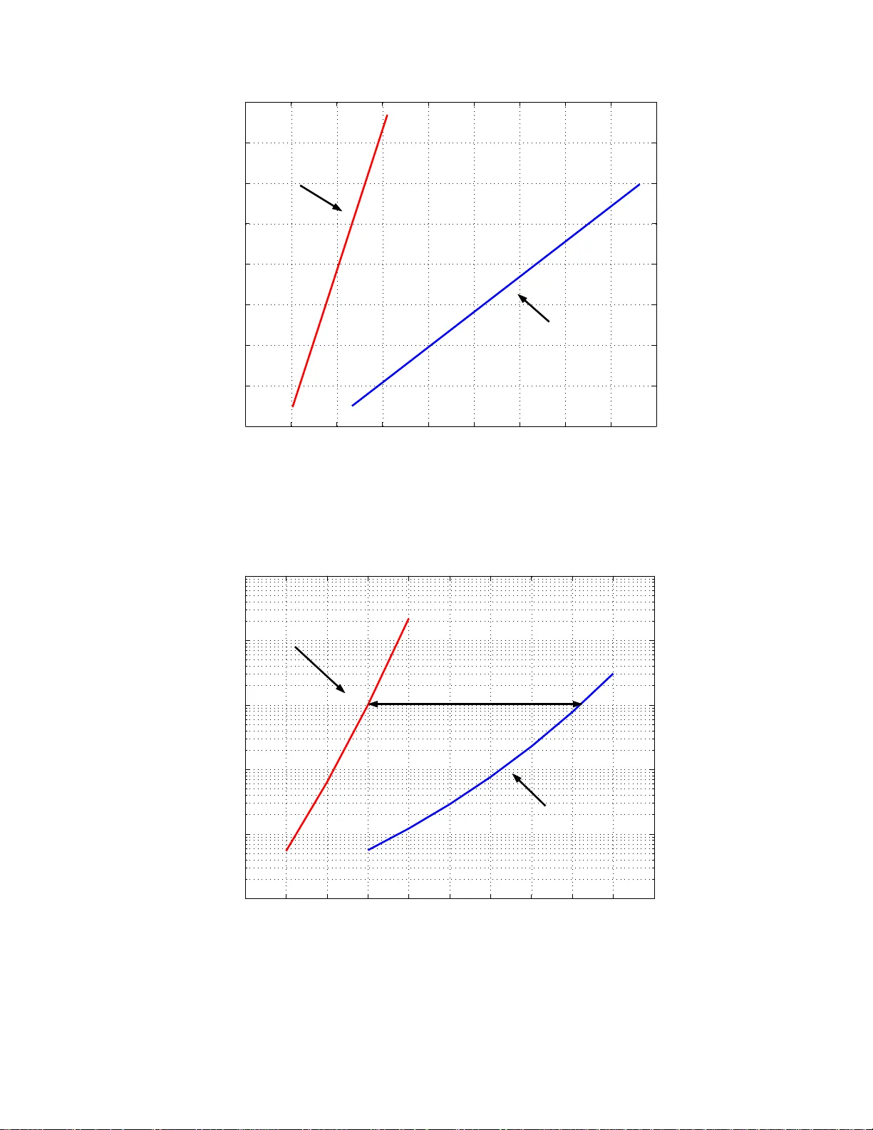
THE EXIT PR OBLEM IN OPTIMAL NON-CA USAL ESTIM A TION D. Ezri ∗ B. Z. Bobrovsky † Z. Sc h uss ‡ July 14, 2021 Abstract W e study the phenomenon of loss of lo c k in the optimal non-causal phase estimation problem, a b enc hm ark p r oblem in n onlinear estima- tion. Our metho d is based on the computation of the asymptotic distribution of the optimal estimation error in case the num b er of tra jectories in the optimization problem is finite. The computation is based directly on th e min imum noise en ergy optimalit y criterion rather than o n s tate equations of t he error, as is the usual case in the literature. The results include an asymptotic computation of the mean time to lose lo ck (MTLL) in the optimal smo other. W e show that the MTLL in the fir st and second order smo others is signifi can tly longer than that in the causal extended Kalman filter. Keyw ords: Nonlinear smo othing, loss of lo c k, cycle slips 1 In tro duc tion In man y applications in commu nication practice a random signal x ( t ) is receiv ed through a noisy c hannel. The random signal x ( t ) ∈ R N is assumed to b e a sto chas tic ∗ Department of E lectrical Eng ineering–Sys tems, T el-Aviv Universit y , Ramat-Aviv, T el- Aviv 69 978, Israel. email: ezri@eng.tau.a c.il † Department of E lectrical Eng ineering–Sys tems, T el-Aviv Universit y , Ramat-Aviv, T el- Aviv 69 978, Israel. email: bo brov@eng.tau.ac.il ‡ Department of Mathematics, T el-Aviv University , Rama t- Aviv , T el-Aviv 69978 , Isra el. email: sch uss@p ost.tau.a c.il 1 pro cess defined b y an Itˆ o sto c hastic differential equation (SDE) [17] d x = m ( x , t ) dt + σ ( x , t ) d w , (1) where w ( t ) is a ve ctor of standard Bro wnian motions. The measuremen ts pro cess y ( t ) ∈ R M , whic h is the output of the noisy c hannel, is mo deled by another SDE d y = g ( x , t ) dt + p N 0 / 2 d v , (2) where N 0 measures the channel noise in tensit y and v ( t ) is another ve ctor of Brow nian motions, indep enden t of w ( t ). W e further assume that the f unctions m ( · , · ) , σ ( · , · ) and g ( · , · ) satisfy standard regularity conditions suc h that ( 1 ),(2) possess a s trong unique solution. When the optimality criterion is minim um square error, the optimal filtering prob- lem is to construct the causal estimator ˆ x ( t ) = E [ x ( t ) | y ( s ) ] of x ( t ), where 0 ≤ s ≤ t [32]. The optimal fixed interv al smo o t hing problem is to construct the non-causal es- timator ˆ x ( t ) = E [ x ( t ) | y ( s ) , 0 ≤ s ≤ T ], where T is the length of the interv al, a nd t < T . The optimal fixed lag smo othing problem is to construct the non- causal esti- mator ˆ x ( t ) = E [ x ( t ) | y ( s ) , 0 ≤ s ≤ t + ∆], where T is the length of the interv a l, and t + ∆ < T . In man y applicatio ns dela y in the estimation of the signal is not p ermis- sible, a s for example in closed-lo op con tro l, radar t rac king systems, a nd so on. There are, how ev er, interes ting cases, where certain dela y is p ermissible, as for example in comm unication systems, as extensiv ely practiced in co ding [34, 20]. Smo others a r e used b ecause their p erfor mance is sup erior to all causal filters, with resp ect to the same optimality criterion [19]. In linear estimation theory , where the optimalit y criterion is minim um mean square error, the error v ariance of the optimal smo other is smaller than that of the o pt imal filter [10]. Optimal estimators are usually infinite-dimensional a nd therefore ha v e no finite- dimensional realizatio ns, so that sub optimal estimators ha ve b een prop osed to approx - imate the optimal ones b y a system of SDEs, driven by the measuremen ts [13 , 21, 22]. The phase-lo c k ed-lo o p (PLL), whic h is a realization of the extended Kalman fil- ter (EKF) [30], is a no nlinear suboptima l causal estimator of the carrier phase in v arious comm unications s ystems [16]. A w ell kno wn effe ct in s uc h PLL demo dula- tors is the cycle slip phenomenon that consists in o ccasional sudde n c ha nges of size 2 π n ( n = ± 1 , ± 2 , . . . ) in the phase estimation error [5]. Ob viously , the mean time b et ween cycle slips, kno wn as the mean time to lose lo c k (MTLL), decreases with the noise in tensit y and causes sharp degradation in the p erforma nce of the filter and t o the f ormation of a p erformance threshold [33, 29, 28]. Considerable effort w as put in to the computation of the MTLL in causal estima- tors [16, 24, 31, 3 3], including the singular p erturbation metho d [28, 29 ] and lar g e deviations theory [9, 8]. Ho we v er, the phenomenon of loss of lo c k in smo others has nev er been address ed, despite the extensiv e study of linear and nonlinear smoothers in the literature [21, 2 2 , 23, 14, 35, 6, 2, 25, 26, 10, 15, 1]. The ob jective of this pap er is to provide the missing theory , estimate the MTLL in the o pt ima l smo other, and compare it with that in the casual PLL. Sp ecifically , w e compute the a symptotic distribution of the optimal estimation error in case the num b er of tra jectories in the 2 optimization problem is finite. W e iden t ify the contribution of error tra jectories to the minimum noise energy (MNE) cost functiona l and recast the problem in t erms of order statistics. The asymptotic expression for the MTLL in the smo other is similar to that resulting f r om the W en tzell-F reidlin theorem for causal systems , with a new functional. Applying our metho d to standard phase mo dels, w e sho w t ha t t he MTLL in the optima l smo other is significan tly longer than that in the PLL. 2 The mathematical mo del The general equations of a scaled phase trackin g system consist of t he linear mo del of the phase x ( t ) = [ x ( t ) , x 2 ( t ) , ..., x N ( t )] T [29] ˙ x = Ax + √ ε B ˙ w (3) and the nonlinear mo del of the noisy measuremen ts y ( t ) = [ y s ( t ) , y c ( t )] T y = h ( x ) + √ ε ˙ v , (4) with h ( x ) =  sin x cos x  . The dimensionless parameter ε is assumed small in t he case of a low noise c hannel [28]. A fixed-in terv al minim um noise energy (MNE) estimator ˆ x ( · ) for x ( · ) is the min- imizer of the cost functional [6] J [ z ( · )] ≡ Z T 0  | y − h ( z ) | 2 + | ζ | 2  dt, (5) with t he equalit y constrain t ˙ z = Az + B ζ , (6) that is, ˆ x ( · ) ≡ a r g min z ( · ) J [ z ( · ) ] . (7) Note that the integral J [ x ( · )] con ta ins the white noises ˙ w ( t ) , ˙ v ( t ), which are not square integrable. T o remedy this problem, we b egin with a mo del in whic h the white noises ˙ w ( t ) , ˙ v ( t ) are replaced with square inte grable wide band noises, and at the appropriate stag e of the analysis, w e tak e t he white noise limit (see b elo w). In con trast to nonlinear filtering, where the lo c k ed state is a lo cal attractor for the error dynamics [29 ], a nd escaping it corresp onds to loss of lo c k, there is no dynamics, and therefore no attractors for smo ot hers. Thus, w e ha v e to define cycle slip ev en ts in a differen t manner than hitting the b oundary of the domain of attractio n. W e define the estimation error e ( t ) = [ e ( t ) , e 2 ( t ) , . . . , e N ( t )] T as e ( t ) = ˆ x ( t ) − x ( t ) , (8) 3 0 1 2 3 4 5 6 7 8 9 10 0 1 2 3 4 5 6 7 t e(t) π t 0 t 0 + ∆ t Figure 1: An example of tw o tr a jec tories in C 1 ( t 0 = 5) and w e sa y that a cycle-slip ha s o ccurred in the time in t erv al ( t 0 , t 0 + ∆ t ) , ∆ t << 1 , if and only if the estimation error e ( t ) v anishes at at some t 0 − T 1 , reac hes the p oint [2 π n, 0 ] T , ( n = ± 1 , ± 2 , ... ), at some later time t 0 + T 2 , and e ( ˜ t ) = π n , where ˜ t ∈ ( t 0 , t 0 + ∆ t ). The time T s = T 1 + T 2 is the slip duration, satisfying T s << T . W e define in the space of con tinuous functions C N [0 ,T ] the set C N ( t 0 ) of all con tinuous tra jectories e ( · ) that slip in the in t erv al ( t 0 , t 0 + ∆ t ). Thus Pr { slip in ( t 0 , t 0 + ∆ t ) } = Pr  e ( · ) ∈ C N ( t 0 )  . (9) F or small v alues of ε the cycle-slip ev en t is a ra re large deviation from the orig ina l tra jectory , and therefore ˆ x ( t ) is in the vicinit y o f x ( t ) b efor e the cycle-slip, and in the vicinity of ˆ x ( t ) + [2 π n, 0 ] T after the slip. Th us, w e can define the b eginning and the end o f the cycle-slip by the instants when e ( t ) reac hes the origin and [2 π n, 0 ] T , resp ectiv ely . An example of t w o t r a jectories in C 1 ( t 0 = 5) is giv en in Fig ure 1. 3 The MTLL in the optimal smo oth er The W en tzell-F reidlin theorem [8, 9] and the singular p erturbation metho d [29] for asymptotic ev aluation of t he MTLL are concerned with sto chastic pro cesses satisfying a sto c hastic differen tial equation with a unique solution. In con t rast, the dynamics of the optimal smo other, deriv ed from the EL equations, form a t wo-po in t b oundary- v alue problem whic h has no unique solution. Therefore the W e n tzell-F reidlin and the singular p erturbatio n method see m inappropriat e for the computation of the MTLL in a smo ot her. It app ears that this computatio n calls fo r a different approac h. 4 The first step tow ard an asymptotic calculation o f the MTLL in smo o thers is the computation of the a symptotic distribution of the estimation error in case t he num b er of tra jectories in the optimization problem is finite. W e in v estigate the cost functional of deterministic error tra jectories that deviate from the original tra jectory x ( t ). W e augmen t x ( t ) with the set of the N T tra jectories r i ( t ) = [ r i ( t ) , r [2] i ( t ) , . . . , r [ N ] i ( t )] ∈ C N [0 ,T ] , i ∈ [1 , . . . , N T ]. The tra jectories x ( t ) + r i ( t ) are admissible in the optimization problem ( 5), (6 ), only if the tra jectories r i ( t ) satisfy ˙ r i = Ar i + B u i . (10) W e define the difference ∆ J [ x ( · ) , r i ( · )] △ = J [ x ( · ) + r i ( · )] − J [ x ( · )] (11) and substitute ( 5), (6 ) and (10) in (11) to o btain ∆ J [ x ( · ) , r i ( · )] = Z T 0 h 4 sin 2  r i 2  + | u i | 2 i dt + √ 4 ε Z T 0 [sin x − sin ( x + r i )] dv 1 ( t ) + √ 4 ε Z T 0 [cos x − cos( x + r i )] dv 2 ( t ) + √ 4 ε Z T 0 u T i d w ( t ) . (12) A t this p oint, w e ta ke the white noise limit in the wide band noises so the sto c hastic in tegrals in (12) b ecome Itˆ o in tegr a ls. Collecting them into a single Itˆ o integral leads to ∆ J [ x ( · ) , r i ( · )] = Z T 0 h 4 sin 2  r i 2  + | u i | 2 i dt + √ 4 ε Z T 0 r 4 sin 2  r i 2  + | u i | 2 d ˜ v i ( t ) , (13) where ˜ v i ( t ) is a standard Brow nia n motion that dep ends on v ( t ) and w ( t ). Note that alt ho ugh the v alues of the random v ariable ∆ J [ x ( · ) , r i ( · )] dep end on the tra jectories of x ( t ) and y ( t ) through v ( t ) and w ( t ), the probability law of ∆ J [ x ( · ) , r i ( · )] dep ends only on the tra jectories r i ( t ). Therefore, w e abbreviate nota- tion to ∆ J [ r i ( · )]. W e no t e further t hat ∆ J [ r i ( · )] is a Gaussian random v ariable with exp ectatio n E∆ J [ r i ( · )] = m i , (14) 5 where m i △ = Z T 0 h 4 sin 2  r i 2  + | u i | 2 i dt, (15) and v ariance V ar { ∆ J [ r i ( · )] } = 4 ε m i . (16) F urthermore, w e compute the co v ariance σ i j = E (∆ J [ r i ( · )] − m i ) (∆ J [ r j ( · )] − m j ) = 4 ε Z T 0 u T i u j dt + 4 ε Z T 0 [1 + cos( r i − r j ) − cos r i − cos r j ] dt. (17) Note that if the supp orts of r i ( · ) and r j ( · ) are disjoin t, the cost functionals ∆ J [ r i ( · )] , ∆ J [ r j ( · )] are not correlated. W e conclu de that the random v ariables ∆ J [ r i ( · )] , i = 1 . . . N T , form a Ga ussian ra ndo m v ector with distribution            ∆ J [ r 1 ( · )] ∆ J [ r 2 ( · )] . . . ∆ J [ r N T ( · )]            ∼ N                                 m 1 m 2 . . . m N T            ; 4 ε            m 1 σ 1 2 . . . ˜ σ 1 N T ˜ σ 1 2 m 2 . . . . . . ˜ σ 1 N T m N T                                 , (18) where ˜ σ ij = 1 4 ε σ ij . When considering a finite n umber of error tra jectories r i ( · ) , i = 1 , . . . , N T in the optimization problem. The es timator error tra j ectory e N T ( · ) minimizes the cost functional ∆ J [ r j ( · )], Pr { e N T ( · ) = r k ( · ) } = Pr { ∆ J [ r k ( · )] < ∆ J [ r j ( · )] f or a ll j 6 = k } . (19) Th us the problem of minimization has b een recast in the languag e of o rder statistics. The probability on the righ t side of (19) is difficult to calculate, so we pursue the distribution of the error tra jectory e N T ( · ) in the limit of small ε . W e assume tha t for eac h k there exists an in terv al A k suc h that E { ∆ J [ r j ( · )] | ∆ J [ r k ( · ) ∈ A k ] } > ∆ J [ r k ( · )] for a ll j 6 = k . (20) Cram ´ er’s theorem f or G aussian vectors [8, 7] implies that in the limit of small ε lim ε → 0 ε log e Pr { ∆ J [ r k ( · )] < ∆ J [ r j ( · )] for all j 6 = k } = lim ε → 0 ε log e Pr { ∆ J [ r k ( · )] ∈ A k } . (21) Next, we ev aluate the conditio nal exp ectatio n E { ∆ J [ r j ( · )] | ∆ J [ r k ( · )] } . (22) 6 Since ∆ J [ r j ( · )] , ∆ J [ r k ( · )] are jo in tly Gaussian, E { ∆ J [ r j ( · )] | ∆ J [ r k ( · )] } = m j + σ j k 4 εm k (∆ J [ r k ( · )] − m k ) = m j + ˜ σ j k m k (∆ J [ r k ( · )] − m k ) . (23) In or der to determine the in terv al A k , defined in (20), we deriv e the set o f N T − 1 inequalities E { ∆ J [ r j ( · )] | ∆ J [ r k ( · )] } > ∆ J [ r k ( · )] f or a ll j 6 = k . (24) The in terv al A k , whic h is the range of v alues of ∆ J [ r k ( · )] satisfying (24) is defined by max r j ( · ) ∈ A − m j − ˜ σ j k 1 − ˜ σ j k m k < ∆ J [ r k ( · )] < min r j ( · ) ∈ A + m j − ˜ σ j k 1 − ˜ σ j k m k , (25) where A + is the set o f all tra j ectories r j ( · ) such that m j < m k , ˜ σ j k > m j , and A − is the set of all tra jectories r j ( · ) suc h that m j > m k , ˜ σ j k > m k . Note that the suprem um and infimum, ov er all con tinuous tr a jectories, of the leftmost and righ tmost sides of (25), resp ectiv ely , is − m k . This means tha t as N T increases a nd the tra j ectories x ( · ) + r i ( · ) are sampled from C [0 ,T ] according to their a priori distribution (3), the in terv al A k narro ws. Sp ecifically , for an y δ, ˜ δ > 0 there is a sufficien tly large N T suc h that Pr { A k 6⊂ ( − m k − δ, − m k + δ ) } < ˜ δ . Com bining (19) and (21), we conclude that fo r all small ε > 0 and ev ery sufficien tly small δ , suc h that 0 < δ < ε , there is a sufficien tly larg e N T suc h that Pr { e N T ( · ) = r k ( · ) } ≍ Pr {− m k − δ < ∆ J [ r k ( · )] < − m k + δ } ≍ 2 δ exp  − 4 m 2 k 8 ε m k  ≍ 2 δ exp  − 1 2 ε Z T 0 h 4 sin 2  r k 2  + | u k | 2 i dt  . (26) Based on the dis tribution of the estimation error e N T ( · ) in the c ase of a finite n umber of error tra jectories N T (26), the probability that e N T ( · ) is in an y set A in C N [0 ,T ] is Pr { e N T ( · ) ∈ A } = X r k ( · ) ∈ A Pr { e N T ( · ) = r k ( · ) } ≍ X r k ( · ) ∈ A 2 δ exp  − 1 2 ε Z T 0 h 4 sin 2  r k 2  + | u k | 2 i dt  . (27) 7 Applying Laplace’s metho d for sums of exp onentials with large pa r a meter 1 ε [3], w e obtain the asymptotic expression Pr { e N T ( · ) ∈ A } ≍ exp  − 1 2 ε min r k ( · ) ∈ A Z T 0 h 4 sin 2  r k 2  + | u k | 2 i dt  . (28) In the limit δ → 0 (a nd N T → ∞ ), the probability that the optimal estimation error e ( · ) is in A is found as Pr { e ( · ) ∈ A } ≍ exp  − 1 2 ε inf r ( · ) ∈ A Z T 0 h 4 sin 2  r 2  + | u | 2 i dt  , (29) sub ject to the equality constrain t ˙ r = Ar + B u , (30) where the infim um in (29) is tak en o ver all con t in uous tra j ectories r ( · ) ∈ A . Note that the small ε approx imation is t a k en b efore the limit δ → 0 . W e turn no w to the computation of the MTLL. First, we consider time in terv als [0 , T ] muc h longer than the time constan t of the sy stem, so that most of the time the system is in steady state. It follows that the pro babilit y Pr { slip in ( t 0 , t 0 + ∆ t ) } is indep enden t of t 0 for t 0 outside in terv als of fixed length (the time constan t of the system) at the endp oin t s 0 and T . Therefore, in view of the regularit y of the p df of the solution as a function of t and the indep endence of cycle slips in disjoint in terv als (see ab o ve), fo r suc h t 0 Pr { slip in ( t 0 , t 0 + 2∆ t ) } = Pr { slip in ( t 0 , t 0 + ∆ t ) } + Pr { slip in ( t 0 + ∆ t, t 0 + 2∆ t ) } + o (∆ t ) = 2 Pr { slip in ( t 0 , t 0 + ∆ t ) } + o ( ∆ t ) . (31) Th us, Pr { slip in ( t 0 , t 0 + ∆ t ) } is nearly linear in ∆ t . Next, w e note that f or fixed ∆ t (29) implies that the slip proba bilit y satisfies Pr { slip in ( t 0 , t 0 + ∆ t ) } = Pr  e ( · ) ∈ C N ( t 0 )  ≍ exp  − 1 2 ε inf r ( · ) ∈ C N ( t 0 ) Z T 0 h 4 sin 2  r 2  + | u | 2 i dt  , (32) sub ject to the equalit y constrain t (30). Equations (31) and (32) can b e written together as Pr { slip in ( t 0 , t 0 + ∆ t ) } = (∆ t + o (∆ t ))Ω( ε ) exp  − inf r ( · ) ∈ C N ( t 0 ) 1 2 ε Z T 0 h 4 sin 2  r 2  + | u | 2 i dt  , (33) 8 sub ject to the equality constrain t (30), where ε log Ω( ε ) → 0 a s ε → 0. Equipped with the slip probabilit y (33), w e turn to the ev aluation of the MTLL in the optimal smo other. W e in tro duce a r enewal (coun ting ) pro cess { N ( t ) , t ≥ 0 } , a nonnegativ e in teger-v alued sto chastic pro cess that coun t s the n um b er successiv e cycle-slip ev ents in the time interv a l (0 , t ] [11]. W e assume that the time durations b et ween consecutiv e slips are p o sitiv e, indep enden t , iden tically distributed random v ariables. Based on the ab ov e a ssumptions, w e adopt the renew al form ula [1 1] τ nc = t E N ( t ) , (34) where τ nc is the MTLL in the non-causal estimator. In the limit of t → ∞ , equation (34) giv es τ nc = lim t →∞ t E N ( t ) = lim t →∞ 1 E ˙ N ( t ) . (35) Using t he slip probability ( 3 3) we obta in E ˙ N ( t ) = lim ∆ t → 0 E  N ( t + ∆ t ) − N ( t ) ∆ t  = lim ∆ t → 0 Pr { slip in ( t 0 , t 0 + ∆ t ) } ∆ t ≍ exp  − inf r ( · ) ∈ C N ( t 0 ) 1 2 ε Z T 0 h 4 sin 2  r 2  + | u | 2 i dt  . (36) Substituting (36) in (35), w e obta in the expression f or the asymptotic MTLL, τ nc , in the o ptimal MNE estimator lim ε → 0 ε log e τ nc = inf e ( · ) ∈ C N ( t 0 ) 1 2 Z T 0 h 4 sin 2  e 2  + | ξ | 2 i dt, (37) sub ject to the equality constrain t ˙ e = Ae + B ξ . (38) 4 The MTLL i n the smo othe r with stand ard phase mo d els W e b egin with the first order phase tra c king sy stem suggested b y [2 7] and [1 8], in whic h the phase x ( t ) is modelled as a standard Brownian motio n ˙ x = ˙ w y = h ( x ) + ρ ˙ v , (39) 9 where x ( t ) , w ( t ) tak e v alues in R 1 . The system (39) is scaled to the fo r m of ( 3), (4) with A = 0 , B = 1 a nd ε = ρ . A similar pro cedure is presen ted in [4 ]. Note that the CNR equals ρ − 2 / 2 in the system (39). In the first order case, the asymptotic expression for the MTLL in the smo o ther (37) b ecomes lim ε → 0 ε log e τ nc = inf e ( · ) ∈ C 1 ( t 0 ) 1 2 Z T 0 h 4 sin 2  e 2  + ˙ e 2 i dt, (40) The v ariationa l problem on the righ t side of (40) is solv ed analytically using t he Hamilton-Jacobi-Belman equation [12 ]. This leads to the asymptotic limit of the MTLL in the first order non-causal estimator as lim ε → 0 ε log e τ nc = lim ρ → 0 ρ log e τ nc = 8 . (41) In order to compare the MTLL in the optimal smo other (41) with that in the sub optimal PLL we construct the steady-state EKF corresp onding to the mo del (39) [30]. ˙ ˆ x = σ ρ ( y s cos ˆ x − y c sin ˆ x ) . (42) The differen tial equation of the causal EKF estimation error e ( t ) = ˆ x ( t ) − x ( t ) is scaled to the form [4] ˙ e = − sin e + √ 2 ε ˙ v . (43) The asymptotic MTLL, τ c , in this simple analytical p otential case is kno wn to b e [29] lim ε → 0 ε log e τ c = lim ρ → 0 ρ log e τ c = 2 . (44) Note that in first order estimators the MTLL in the non-causal estimator (41) is significan tly longer than that in the causal estimator (44). This implies that the CNR v alues in the smo other are smaller than in the filter, but giv e a MTLL iden tical to that in the filter. Denoting b y ε c , ε nc the v alues of ε in the filter a nd smoother, resp ectiv ely , a nd requiring iden tical MTLLs, lead to τ c = τ nc ⇒ 2 ε c = 8 ε nc . (45) Denoting b y CNR c [dB] , CNR nc [dB] the CNR in the filter a nd smo other, resp ectiv ely , and using the simple relation b et w een ε and the CNR, lead to CNR c [dB] − CNR nc [dB] = 10 · 2 log 10 (8 / 2) ≈ 1 2dB . (46) Th us, there exis ts a 12 dB p erformance gap in the MTLL b et w een the estimators in terms of CNR. The MTLL in first order non-causal MNE smo o ther and causal EKF are given in Figures 2 and 3 . The pre-expo nen tial term in the plots is arbitra r y . 10 2 2.5 3 3.5 4 4.5 5 5.5 6 6.5 2.5 3 3.5 4 4.5 5 5.5 6 6.5 1/ ε =1/ ρ log 10 MTLL Smoother PLL Figure 2: The MTLL in the first o rder optimal MNE estimator and the causal PLL as a function of 1 /ε . 4 5 6 7 8 9 10 11 12 13 14 10 2 10 3 10 4 10 5 10 6 10 7 CNR[dB] MTLL Smoother PLL ∆ CNR → 12 dB Figure 3: The MTLL in the first o rder optimal MNE estimator and the causal PLL as a function of the CNR. 11 Next we consider the more complex, and more realistic, case of a second order phase mo del [3 0], in whic h the phase is mo delled a s an integral o v er a Brownian motion. The signal mo del is ˙ x = A ′ x + B ′ ˙ w , (47) where A ′ =  0 1 0 0  , B ′ =  0 0 0 1  . The measuremen ts mo del is y = h ( x ) + ρ ˙ v , (48) where x ( t ) and w ( t ) take v alues in R 2 . The system (4 7), (48) is scaled to the form o f (3),(4) with A = A ′ , B = B ′ , and ε = ρ 3 / 2 . Note t hat in this case the CNR equals ρ − 2 / 2, as in the case of the first order system. In the second order case, the asymptotic expression for the MTLL in t he smo other (37) b ecomes lim ε → 0 ε log e τ nc = inf e ( · ) ∈ C 2 ( t 0 ) 1 2 Z T 0 h 4 sin 2  e 2  + ¨ e 2 i dt, (49) v ariational problem on the r ig h t side of (37) as no analytical solution. An ap- pro ximate solution is obta ined nume rically ab out the characteris tics of the Hamilton- Jacobi-Belman equation [29 , 5]. This leads to the asymptotic limit of the MTLL in the second or der non-causal estimator as lim ε → 0 ε log e τ nc = lim ρ → 0 ρ 3 / 2 log e τ nc = 5 . (50) W e note tha t the EKF corresp onding to the second order system (4 7), (48) has the erro r equations [30 ],[5] ˙ e = 1 2 ϕ − sin e − √ 2 ε ′ ˙ v ˙ ϕ = − sin e − √ 2 ε ′ ˙ v + √ 2 ε ′ ˙ w , (51) where ε ′ = ε/ √ 2. The ” eik onal” equation [5 ] for the quasi-p otential Φ corresp onding to (5 1) is  1 2 ϕ − sin e  Φ e − sin e Φ ϕ + Φ 2 e + 2Φ e Φ ϕ + 2Φ 2 ϕ = 0 . (52) The function Φ is ev aluated n umerically on t he characteris tics of (52) [5]. This pro cedure leads to the v alue of the quasi-p otential at the unstable equilibrium p o in t Φ( ϕ = 0 , e = π ) = 0 . 6, so the asymptotic MTLL in the second o r der causal estimator is lim ε → 0 ε log e τ c = lim ρ → 0 ρ 3 / 2 log e τ c = 0 . 85 . (53) 12 2 4 6 8 10 12 14 16 2.5 3 3.5 4 4.5 5 5.5 6 1/ ε =1/ ρ 3/2 log 10 (MTLL) Smoother PLL Figure 4: The MTLL in the second order optimal MNE estimator and the causal PLL as a function of 1 / ε . Note that sim ilarly to the first or der case, the MTLL in the sec ond order smoo t her (50) is significan tly longer than that in the causal PLL ( 5 3). The CNR g a p in this case is CNR c [dB] − CNR nc [dB] = 40 / 3 log 10 (5 / 0 . 85) ≈ 10 . 25dB . (54) The MTLL in t he non-causal estimator and the causal EKF in the second order system are given in Figures 4 and 5 . The pre-expo nen tial term in the plots is arbitra r y . 5 Discuss ion and c onclus ions The significan t adv an tage of the optima l smo other o v er the causal PLL defies in t u- ition. It w as customary to think that the MTLL adv an tag e o f the smo other is linke d and prop ortional to the MSE adv a ntage o f the smoo ther [32]. W e argue that the MSE in an estimator is not related to the MTLL. In order to demonstrate this idea w e in tr o duce the follow ing error equation ˙ e = − 2 sin e 2 + √ ε ˙ ˜ v . (55) The MSE in the linearized version of (55) is iden tical to that in linearized v ersion of the system ˙ e = − sin e + √ ε ˙ ˜ v . (56) 13 3 4 5 6 7 8 9 10 11 12 13 10 2 10 3 10 4 10 5 10 6 CNR[dB] MTLL Smoother PLL ∆ CNR → 10.25 dB Figure 5: The MTLL in the second order optimal MNE estimator and the causal PLL as a function of CNR. Ho we v er, due to t he difference in the p oten tia l barrier in the ab o v e systems, the asymptotical MTLL, τ 1 , in the system (55) satisfies lim ε → 0 ε log e τ 1 = 1 2 inf { e (0)=0 , e ( T ′ )=2 π } Z T ′ 0  ˙ e + 2 sin e 2  2 dt = 8 , (57) while the MTLL, τ 2 , in the system (56) satisfies lim ε → 0 ε log e τ 2 = 4 , (58) and is significan tly shorter than τ 1 . Thus , we conclude that the MTLL adv an tage of the o ptimal smoo ther o ver the PLL is due to an entirely differen t functional and cannot b e predicted by the MSE adv an tage of the smo other o ver the filter. There is a fundamen tal mathematical difference b et wee n the causal and the no n- causal cases. Both problems inv olv e the minimization of a f unctional, similar to that of the W en tzell-F reidlin theory for causal systems. There is, ho w eve r, a differe nce b et ween the functionals in the t wo theories. While the functional in the causal case v anishes along the exiting tra jectories from the b oundary of the domain of attra ction of the lo ck ed state to the next lo c ked state [9], in the non-causal cas e the functional v anishes only at the lo c ke d states, so it has to b e computed along the entire slip tra jectory . 14 References [1] Anderson, B.D.O. Fixed in terv al smo othing for nonline ar con tin uous time systems. J. In fo. Contr ol , 20:294–30 0, 1972. [2] Bellman, R., Kalba , R., and Middelton, D. Dynamic programming, sequen tial estimation and sequen tial detection pro cesses. Pr o c. Nat. A c ad. Sci.U.S.A. , 47:33834 1, 1961. [3] Bender, C.M., and Orszag, S.A. A dvanc e d Mathematic al Met ho ds for Scientists and Engine ers . Springer, New Y ork, 1999 . [4] Bobrovsky , B.Z ., and Sc h uss, Z . Singular p erturbation in filtering the- ory . IF AC Worksho p on singular p erturb ations in optimal c ontr ol , pages 1439–144 7, June 1978. [5] Bobrovsky , B.Z., and Sc huss , Z. A singular p erturbation metho d for the computation of the mean first passage time in a non linear filter. SIAM , 42(1):174– 187, F eb. 1982. [6] Bryson, A.B., and Ho, Y.C. Applie d Optima l Contr ol . John Wiley , New Y ork, 1975. [7] Buck lew, J.A. L ar ge Deviation T e chniques in De cision, Sim ulation and Estimation . Wiley , New Y ork, 1990. [8] D em b o , A., and Z eitouni, O. L ar ge Devia tions T e c hniques and Applic a- tions . Jones and Bartlett, 19 9 3. [9] F reidlin, M.A., a nd W en tzell, A.D. R ando m Perturb ations of Dynamic al Systems . Springer-V erlag, New Y ork, 1984. [10] K a ilath, T., and F rost, P . An innov atio n approac h to least-squares estimation part II: Linear smo othing in addativ e white noise. IEEE T r ans. A uto. Contr onl , A C-13 :655–660 , 1968. [11] K a rlin S., and T aylor, H.M. A F i rs t Course in Sto chastic Pr o c esses . Academic Press, 1975. [12] K ir k D.E. Optimal Contr ol The ory - an Intr o duction . P ren tice-Hall, Inc., 1970. [13] K ushner, H.J. Dynamical equations f o r optimal nonlinear filtering. J. Diff. Equations , 2:1 79–190, 1967. [14] Lee, R.C.K. Op tima l Estimation Idetific ation and Contr ol . M.I.T. Press, 1964. [15] Leondes, C.T., Pelle r, J.B., and Stear, E.B. Nonlinear smo othing theory. IEEE T r ans. Sys. Sc i . Cyb. , SSC-6:6 3–71, 1970. 15 [16] Lindsey , W.C. Synchr onization Systems in Communic ation a nd Contr ol . Pren tice-Hall, Englew o o d Cliffs, 1972. [17] Lipt ser, R .S., and Shiry a yev , A.N. Stat istics o f R andom Pr o c esses , vol- ume I,I I. Springer-V erlag, New Y ork, 1977. [18] Macchi, O., and Sc harf, L.L. A dynamic programming algorithm for phase estimation and da t a deco ding on random phase c hannels. I EEE T r ans. Info. The ory , IT-2 7(5):585–5 95, Sept. 1981. [19] Meditch , J.S. A surv ey of data smo othing for linear and nonlinear dy- namic systems. A utomatic a , 9:15 1–160, 1 9 73. [20] Proa kis, J.G. Digital Comm unic ations . McGra w-Hill, 4th edition, 20 01. [21] R auc h, H.E. Linear estimation of sampled sto chastic pro cesses with random pa r a meters. T ec hnical Rep ort 210 8 , Sta nf o rd Electronics Labra- tory , Stanford Univ ersit y , California, 1962. [22] R auc h, H.E. Solutions to the linear sm o othing problem. I EEE T ans. A uto. Contr ol. , A C-8:371–372 , 1963. [23] R auc h, H.E., T ung, F., and Steib el, C.T. Maxim um lik eliho o d estimates of linear dynamic systems. AI AA J. , 3:1 445–145 0, 1965. [24] R yter, D., and Meyr, H. Theory of phase track ing systems of arbitrary order. IEEE T r ans. Info. The ory , IT-24:1–7, 1978. [25] Sa g e, A.P . Maxim um a p o steriori filtering and smo othing algorit hms. Int. J. Contr ol , 11 :171–183, 1970. [26] Sa g e, A.P ., and Ewing, W.S. On filtering and smo othing algorithms for nonlinear state estimation. Int. J. Contr ol , 11:1–1 8 , 19 7 0. [27] Scharf, L.L., Co x, D.D., and Masreleiz, C.J. Mo dulo 2 π phase sequence estimation. IEEE T r ans. Inf o . The ory , IT-26(5):615–62 0, Sept. 1980. [28] Sch uss, Z. Singular p erturbation metho ds in sto c hastic differen tial equa- tions of mathematical ph ysics. SIAM , Rev 22:119–15 5 , 1 980. [29] Sch uss, Z . The ory and Applic ations of Sto chastic Diff er ential Equations . John Wiley , New Y ork, 1980. [30] Snyde r, D.L. The State V ariable Appr o ach to Continuous Est imation . The M.I.T Press, 196 9. [31] T a usworth, R. Cycle slipping in phase lo c ked lo o ps. IEEE T r ans. Comm. , COM-15:417–421 , 1967. 16 [32] V an T rees, H.L. D e te ction, Estimation and Mo dulation The ory , v ol- ume I I. John Wiley , New Y ork, 1970. [33] Viterbi, A.J. Princ iples of Coher ent Communic ation . McGraw-Hill, New Y ork, 1966. [34] Viterbi, A.J., and Om ura, J.K. Principles of Dig i tal Com munic ation and Co ding . McGraw-Hill, 197 9. [35] W eav er, C.S. Estimating the output of a line ar disc rete system with Gaussian input. IEEE T r ans. Auto. Contr ol , AC -8:372–3 74, 1963 . 17