Dynamic generalized linear models for non-Gaussian time series forecasting

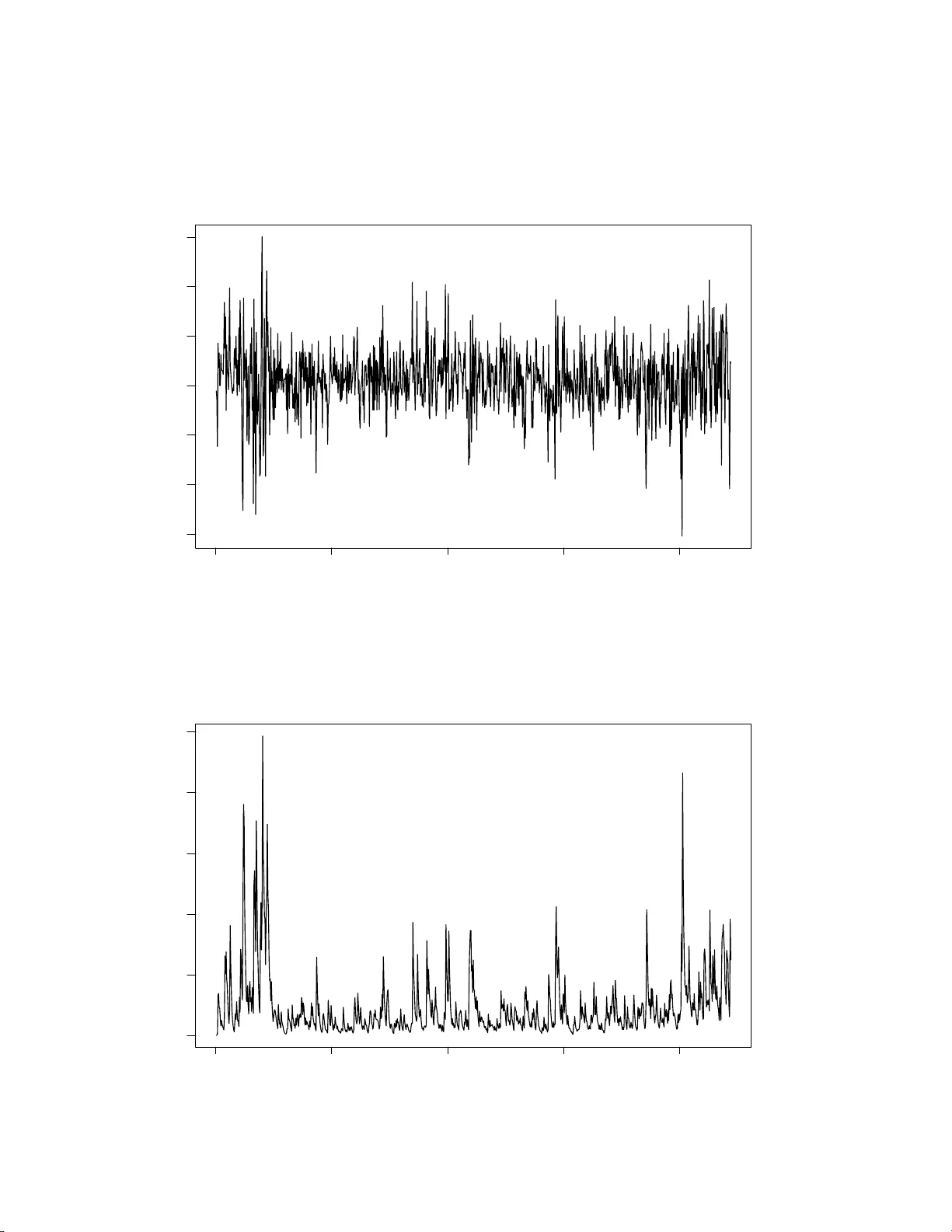
Dynamic generalized linear mo dels for non-Gaussian time series forecasting K. T rian tafyllop oulos ∗ F ebruary 11, 2013 Abstract The purp o se of this pap er is to provide a discussion, with illustrating ex amples, on Bay esian forecasting fo r dynamic generalized linear mo dels (DGLMs). Adopting appr o x- imate B a yesian analysis, ba sed o n conjugate fo rms and on Bayes linear estimation, we describ e the theoretical fra mew ork and then we provide detailed examples of r espo nse dis- tributions, including binomial, Poisson, negative binomial, geo metric, nor mal, log-normal, gamma, exp onent ial, W eibull, Pareto, be ta , and inv erse Ga ussian. W e giv e n umerical il- lustrations for all distributions (except for the normal). Putting together all the above distributions, we give a uniﬁed Bay esian approach to no n-Gaussian time serie s analy- sis, with applications from ﬁnance and medicine to biology and the b ehavioural sciences. Throughout the mo dels w e discuss Ba yesian foreca sting and, for eac h model, we deriv e the m ulti-step forecast mea n. Finally , we des cribe mo del assessment using the likelihoo d function, and Bayesian model monitoring. Some key w or ds: Bay es ian forecasting, non-Gaussian time ser ies, dyna mic gener alized linear model, state space, K alman ﬁlter. 1 In tro duction In the past three decades n on-Gaussian time series ha v e attracted a lot of inte rest, see e.g. Co x (1981 ), Kaufmann (198 7), Kitag a w a (1987 ), Sheph ard and Pitt (19 97), and Durbin and Ko opman (2000), among others. In the conte xt of regression mo delling, generalize d linear models (McCullag h and Nel der, 1989; Dobson, 2002) oﬀer a solid theoretical basis for statistic al analysis of ind ep enden t n on-normal data. A general f r amew ork for dealing with time series d ata is the dynamic generalize d linear mod el (DG LM), whic h considers generalized linear mo delling with time-v arying p arameters and hence it is capable to mo del time s eries data for a wide range of resp onse distributions. DGLMs ha v e b een wid ely adopted f or non- normal time series data, s ee e.g. W est et al. (1985), Gamerman and W est (1987), F ahrmeir (1987 ), F r ¨ uhwirth-Sc hn atter, S. (199 4), Lindsey and Lam b ert (1995), Chiogna an d Gaetan (2002 ), Hemming and Shaw (2002), Go dolphin and T rian tafyllop oulos (2006), and Gamerman (1991 , 1998 ). Dynamic generalized linear mo dels are rep orted in detail in the monographs of W est and Harrison (1997, Ch apter 14), F ahrmeir an d T utz (2001, Ch apter 8), and Kedem and F okianos (2002, Ch apter 6). ∗ Department of Probabilit y and Statistics, H ic ks Building, Universit y of Sheﬃeld, Sheﬃeld S3 7RH, UK, email: k.triantafyllopou los@sheffield.ac. uk 1 In this pap er w e prop ose a un iﬁed treatmen t of DGLMs that includes appro ximate Ba y esian inference and m ulti-step forecast ing. In this to end w e adopt the estimation approac h of W est et al. (1985), bu t we extend it as far as mo del d iagnostic s and forecasting are concerned. In particular, we discuss lik eliho o d-based m od el assessmen t as w ell as Ba y esian mo del mon- itoring. In the literature, discussion on th e DGLMs is u sually restricted to the binomial and the Poisson mo d els, see e.g. F ahrmeir and T utz (2001, C hapter 8). Even for these r e- sp onse distributions, d iscussion is limited on estimation, wh ile f orecasting and in p articular m ulti-step forecasting d oes not app ear to ha v e receiv ed m uc h atten tion. W e pro vide detailed examples of man y d istributions, including binomial, P oisson, negat iv e binomial, geometric, normal, log-normal, gamma, exp onen tial, W eibull, P areto, t w o sp ecial cases of the b eta, and in v erse Gaussian. W e giv e numerical illustrations for all distributions, except for the norm al (for whic h one can ﬁnd n umerous illustrations in th e time series literat ure) us in g real and sim ulated data. The pap er is organized as follo ws. In Section 2 we discuss Ba y esian inference of DGLMs. Section 3 commences by considering seve ral examples, where the resp ons e time series follo ws a particular distribu tion. Sectio n 4 giv es concludin g commen ts. T h e app endix includes some pro ofs of argument s in Section 3. 2 Dynamic generalized linear mo dels 2.1 Mo del deﬁnition Supp ose that the time series { y t } is generated from a pr obabilit y distribution, which is a mem b er of the exp onenti al family of d istributions, that is p ( y t | γ t ) = exp  1 a ( φ t ) ( z ( y t ) γ t − b ( γ t ))  c ( y t , φ t ) , (1) where γ t , kno wn as the natural parameter, is th e parameter of in terest and other parameters that can b e link ed to φ t , a ( . ), b ( . ) and c ( ., . ) are usu ally referred to as nuisance parameters or h yp erparameters. The functions a ( . ), b ( . ) and c ( ., . ) are assum ed kno wn, φ t , a ( φ t ) , c ( y t , φ t ) > 0, b ( γ t ) is t wice diﬀerenti able and according to Dobson (2002, § 3.3) E ( z ( y t ) | γ t ) = db ( γ t ) dγ t and V ar( z ( y t ) | γ t ) = a ( φ t ) d 2 b ( γ t ) γ 2 t . The function z ( . ) is usually a simple function in y t and in man y cases it is the iden tit y function; an exception of this is the binomial distribu tion. If z ( y t ) = y t , distribution (1) is said to b e in the c anonic al or standar d form. Dobson (2002, § 3.3) giv es expressions of the score statistics and the information matrix, although the consideratio n of these m a y not b e n ecessary for Ba yesian inference. The idea of generalized linear m o d elling is to use a non-linear fun ction g ( . ), whic h maps µ t = E ( y t | γ t ) to the linear predictor η t ; this function is kno wn as link function. I f g ( µ t ) = γ t , this is r eferred to as c anonic al link , b ut other links may b e more u seful in applications (see e.g. the inv erse Gaussian example in Section 3.2). In GLM theory , η t is mo delled as a linear mo del, but in DGLM theory , the linear predictor is replaced by a state space mo del, i.e. g ( µ t ) = η t = F ′ t θ t and θ t = G t θ t − 1 + ω t , 2 where F t is a d × 1 d esign v ector, G t is a d × d evoluti on matrix, θ t is a d × 1 r andom v ector and ω t is an inno v ation v ector, w ith zero mean and some known co v ariance m atrix Ω t . It is assumed that ω t is uncorrelated of ω s (for t 6 = s ) and ω t is uncorrelated of θ 0 , f or all t . It is ob vious th at if one sets G t = I p (the d × d iden tit y matrix) and ω t = 0 (i.e. its co v ariance matrix is the zero matrix), then the ab o v e mo del is red u ced to a u sual GLM. F or the examples of Section 3 we consider simple state space mo dels, whic h assume that F t = F , G t = G , Ω t = Ω are time-in v ariant. Ho wev er, in the next sections, w e present Ba yesian inference and forecasting f or time-v arying F t , G t , Ω t in order to co v er the general situation. 2.2 Ba y esian inference Supp ose that we ha v e d ata y 1 , . . . , y T and we form the information set y t = { y 1 , . . . , y t } , for t = 1 , . . . , T . A t time t − 1 we assu me that the p osterior mean vec tor and co v ariance matrix of θ t − 1 are m t − 1 and P t − 1 , resp ectiv ely , and we wr ite θ t − 1 | y t − 1 ∼ ( m t − 1 , P t − 1 ). Then fr om θ t = G t θ t − 1 + ω t , it follo ws that θ t | y t − 1 ∼ ( h t , R t ), w h ere h t = G t m t − 1 and R t = G t P t − 1 G ′ t + Ω t . The n ext step is to f orm the prior mean and v ariance of η t and θ t , that is  η t θ t      y t − 1 ∼  f t h t  ,  q t F ′ t R t R t F t R t  , (2) where f t = F ′ t h t and q t = F ′ t R t F t . The quan tities f t and q t are the forecast mean and v ariance of η t . In order to pro ceed with Ba yesian inference, w e assu me the conjugate prior of γ t , so that p ( γ t | y t − 1 ) = κ ( r t , s t ) exp( r t γ t − s t b ( γ t )) , (3) for some kno wn r t and s t . These p arameters ca n b e found from g ( µ t ) = η t and f t = E ( η t | y t − 1 ), q t = V ar( η t | y t − 1 ), whic h are kno wn from (2). The n ormalizing constan t κ ( ., . ) can b e found b y κ ( r t , s t ) =  Z exp( r t γ t − s t b ( γ t )) dγ t  − 1 , where the int egral is Leb esque integ ral, so that it includes summation / int egration of discrete / cont in uous v ariables. W e n ote that in most of th e cases, the ab o ve distribu tion will b e recognizable (e.g. gamma, b eta, normal) and so there is no need of ev aluating the ab o v e in tegral. One example that this is not the case is the inv erse Gaussian d istrib ution (see Section 3.2). Then observing y t , the p osterior distribution of γ t is p ( γ t | y t ) = p ( y t | γ t ) p ( γ t | y t − 1 ) R p ( y t | γ t ) p ( γ t | y t − 1 ) dγ t = κ  r t + z ( y t ) a ( φ t ) , s t + 1 a ( φ t )  exp  r t + z ( y t ) a ( φ t )  γ t −  s t + 1 a ( φ t )  b ( γ t )  . (4) In man y situations we are int erested in parameters that are giv en as functions of γ t . In suc h cases w e d eriv e the prior/p osterior distributions of γ t as ab ov e and then w e apply a transformation to obtain the prior/p osterior distribution of the p arameter in in terest. The examples of Section 3 are illuminativ e. 3 Finally , th e p osterior mean vect or and co v ariance matrix of θ t are approximat ely giv en b y θ t | y t ∼ ( m t , P t ) , (5) with m t = h t + R t F t ( f ∗ t − f t ) /q t and P t = R t − R t F t F ′ t R t (1 − q ∗ t /q t ) /q t , where f ∗ t = E ( η t | y t ) and q ∗ t = E ( η t | y t ) can b e found from g ( µ t ) = η t and the p osterior (4). The priors (2), (3) and the p osteriors (4), (5) provide an alg orithm for estimation, for an y t = 1 , . . . , T . F or a pro of of the ab ov e algorithm the r eader is referred to W est et al. (1985) . An alternativ e app roac h for the sp eciﬁcation of r t and s t is to mak e u se of p ower dis- c ounting and this is b rieﬂy discussed next. T he idea of p o w er discounting stem in the w ork of Smith (1979); p ow er discoun ting is a metho d of obtaining the pr ior distribution at time t + 1, from the p osterior distribu tion at time t . Here we consider a m inor extension of the metho d b y replacing t + 1 by t + ℓ , for some p ositiv e integ er ℓ . Then, according to the pr in ciple of p o w er discount ing, the prior distribution at time t + ℓ is prop ortional to ( p ( γ t | y t )) δ , where δ is a discount factor. T h us w e write p ( γ t + ℓ | y t ) ∝ ( p ( γ t ) | y t ) δ , for 0 < δ < 1 . This ensures that the prior distribution of γ t + ℓ is ﬂatter than the p osterior d istribution of γ t . The ab ov e pro cedur e assu mes th at r t ( ℓ ) = r t +1 and s t ( ℓ ) = s t +1 , whic h implicitly assumes a random w alk t yp e ev olution of the p osterior/prior up dating, in the sense that Ba ye s decisions in the in terv al ( t, t + ℓ ) remain constant, w hile the resp ectiv e exp ected loss (under step loss functions) increase (Smith, 1979). 2.3 Ba y esian forecasting and mo del assessme n t Supp ose that the time series { y t } is generated by den s it y (1) and let y t b e the information set u p to time t . Then the ℓ -step forecast distribu tion of y t + ℓ is p ( y t + ℓ | y t ) = Z p ( y t + ℓ | γ t + ℓ ) p ( γ t + ℓ | y t ) dγ t + ℓ = κ ( r t ( ℓ ) , s t ( ℓ )) c ( y t + ℓ , φ t + ℓ ) κ  r t ( ℓ ) + z ( y t + ℓ ) a ( φ t + ℓ ) , s t ( ℓ ) + 1 a ( φ t + ℓ )  , (6) where r t ( ℓ ) and s t ( ℓ ) are ev aluated from f t ( ℓ ) and q t ( ℓ ), the mean and v ariance of η t + ℓ | y t , and th e distribution of γ t + ℓ | y t , which tak es a similar f orm as the d istribution of γ t | y t − 1 . Mo del assessmen t can b e done via th e lik elihoo d function, residual analysis, and Ba yesian mo del comparison, e.g. based on Bay es factors. T he lik eliho o d fun ction of γ 1 , . . . , γ T , based on inform ation y T is L ( γ 1 , . . . , γ T ; y T ) = T Y t =1 p ( y t | γ t ) p ( γ t | γ t − 1 ) , where the ﬁrst probabilit y in the pr od uct is th e distribution (1) and the second indicates the ev olution of γ t , giv en γ t − 1 . Then the log-lik eliho o d function is ℓ ( γ 1 , . . . , γ T ; y T ) = T X t =1  1 a ( φ t ) ( z ( y t ) γ t − b ( γ t )) + log c ( y t , φ t )  + T X t =1 log p ( γ t | γ t − 1 ) . (7) The lik elihoo d function can b e used as a means of mo del comparison (for example looking at t w o mo del sp eciﬁcat ions, whic h diﬀer in some qu an titat iv e parts, we choose the mo del th at 4 has larger lik eliho od ). F or mo d el assessmen t the lik eliho o d function can b e used in ord er to c ho ose some hyperp arameters (discoun t factors, or n uisance parameters) so that the lik eliho o d function is maximized in terms of these hyp erparameters. The ev aluation of (7) requires the distribution p ( γ t | γ t − 1 ). This dep ends on the state space mo del for η t used. In the examples of Section 3 we look at these probabilities, b ased mainly on Gaussian random walk ev olutions for η t , but also we consider a linear trend mod el for η t . Not e that th e consideration of ω t follo win g a Gaussian distribu tion d o es not imply th at θ t | y t follo ws a Gaussian d istrib ution to o, since the distribution of θ 0 ma y not b e Gaussian. F or the sequenti al calculati on of the Ba y es factors (whic h for Gaussian resp onses are discussed in Salv ador and Gargal lo, 2005), a t ypical setting s u ggests the formation of t wo mo dels M 1 and M 2 , whic h diﬀer in s ome quantita tiv e asp ects, e.g. some hyp erparameters. Then, the cumulat iv e Ba y es factor of M 1 against M 2 is deﬁn ed by H t ( k ) = p ( y t , . . . , y t − k +1 | y t − k , M 1 ) p ( y t , . . . , y t − k +1 | y t − k , M 2 ) = H t − 1 ( k − 1) H t (1) = t Y i = t − k + 1 H i (1) (8) where H 1 (1) = H t (0) = 1, for all t , and p ( y t , . . . , y t − k +1 | y t − k , M j ) denotes the join t distribu - tion of y t , . . . , y t − k +1 , give n y t − k , for some inte ger 0 < k < t and j = 1 , 2. T hen preference of mo del 1 w ould imply larger forecast distribu tion of this mo del (or H t ( k ) > 1); lik ewise preference of mo del 2 w ould imply H t ( k ) < 1; H t ( k ) = 1 implies that the t wo mod els are probabilistically equiv alen t in the sense they pro vide the same forecast distributions. 3 Examples 3.1 Discrete distr ibutions for the response y t 3.1.1 Binomial The b inomial distribu tion (Johnson et al. , 2005) is p erhaps the most p opu lar discrete distri- bution. It is t ypically generated as the su m of indep enden t success/failure b ernoulli trials and in the con text of generalized linear mo delling is asso ciated with logistic r egression (Dobson, 2002) . Consider a discrete-v alued time series { y t } , wh ic h, for a giv en probabilit y π t , f ollo ws the binomial d istribution p ( y t | π t ) =  n t y t  π y t t (1 − π t ) n t − y t , y t = 0 , 1 , 2 , . . . , n t ; n t = 1 , 2 , . . . ; 0 < π t < 1 , where  n t y t  denotes the b inomial co eﬃcien t. It is easy to ve rify that the ab ov e distribution is of the form (1) with z ( y t ) = y t /n t , γ t = log π t / (1 − π t ), a ( φ t ) = φ − 1 t = n − 1 t , b ( γ t ) = log(1 + exp( γ t )), and c ( γ t , φ t ) =  n t y t  . Th e logarithmic, kn o w n also as logit, link η t = g ( µ t ) = γ t = log π t / (1 − π t ) maps π t to the linear p redictor η t , which with the setting η t = F ′ θ t and θ t = Gθ t − 1 + ω t , generates the dynamic ev olution of the mo del. The pr ior of π t | y t − 1 , follo ws by the pr ior of γ t | y t − 1 and the transformation γ t = log π t / (1 − π t ) as b eta distribution π t | y t − 1 ∼ B ( r t , s t − r t ), w ith density p ( π t | y t − 1 ) = Γ( s t ) Γ( r t )Γ( s t − r t ) π r t − 1 t (1 − π t ) s t − r t − 1 , 5 where Γ( . ) denotes the gamma function and s t > r t > 0. Then, observ in g y t , the p osterior of π t | y t is π t | y t ∼ B ( r t + y t , s t + n t − r t − y t ). In the app endix it is sho wn that, with f t and q t the pr ior mean and v ariance of η t , an appro ximation of r t and s t is giv en by r t = 1 + exp( f t ) q t and s t = 2 + exp( f t ) + exp( − f t ) q t . (9) In order to pro ceed with the p osterior momen ts of θ t | y t as in (5), we can see that f ∗ t = ψ ( r t + y t ) − ψ ( s t − r t + n t − y t ) and q ∗ t = dψ ( x ) dx     x = r t + y t + dψ ( x ) dx     x = s t + n t − y t , where ψ ( . ) d enotes the digamma function (see the P oisson example and the app endix). In the app endix approxima tions of ψ ( . ) and of its ﬁrst deriv ativ e (also kno wn as trigamma function) are giv en . These d eﬁnitions as wel l as the parameters of the b eta prior are slightl y diﬀeren t from the ones obtai ned by W est and Harrison (1997) , as these authors use a d iﬀeren t parameterizati on, whic h d o es not app ear to b e consisten t with the pr ior/p osterior up dating. Giv en in formation y t , the ℓ -step forecast d istribution is obtained b y ﬁ rst noting th at π t + ℓ | y t ∼ B ( r t ( ℓ ) , s t ( ℓ ) − r t ( ℓ )) , (10) where r t ( ℓ ) and s t ( ℓ ) are give n by r t and s t , if f t and q t are replaced by f t ( ℓ ) = E ( η t + ℓ | y t ) and q t ( ℓ ) = V ar( η t + ℓ | y t ), w h ic h are calculated r outinely b y the Kalman ﬁlter (see S ecti on 2). Then the ℓ -step forecast distribution is giv en by p ( y t + ℓ | y t ) = Γ( s t ( ℓ )) Γ( r t ( ℓ ))Γ( s t ( ℓ ) − r t ( ℓ ))Γ( s t ( ℓ ) + n t + ℓ ) × 1 n t + ℓ  n t + ℓ y t + ℓ  Γ( r t ( ℓ ) + y t + ℓ )Γ( s t ( ℓ ) − r t ( ℓ ) + n t + ℓ − y t + ℓ ) . W e can use conditional exp ectations in order to calculate the forecast mean and v ariance, i.e. y t ( ℓ ) = E ( y t + ℓ | y t ) = E ( E ( y t + ℓ | π t + ℓ ) | y t ) = n t + ℓ ( r t ( ℓ ) + 1) r t ( ℓ ) + s t ( ℓ ) + 1 and V ar( y t + ℓ | y t ) = E (V ar( y t + ℓ | π t + ℓ ) | y t ) + V ar ( E ( y t + ℓ | π t + ℓ )) = n t + ℓ ( r t ( ℓ ) + 1) r t ( ℓ ) + s t ( ℓ ) + 1 − n t + ℓ ( r t ( ℓ ) + 1)( r t ( ℓ ) + 2) ( r t ( ℓ ) + s t ( ℓ ) + 1)( r t ( ℓ ) + s t ( ℓ ) + 2) + n 2 t + ℓ ( r t ( ℓ ) + 1) s t ( ℓ ) ( r t ( ℓ ) + s t ( ℓ ) + 1) 2 ( r t ( ℓ ) + s t ( ℓ ) + 2) F or the sp eciﬁcation of r t and s t , we can alternativ ely use p o wer discoun ting (see S ection 2). Th is yields r t +1 = δr t + δ y t + 1 − δ and s t +1 = δ s t + δ n t + 2 − δ, where δ is a discount factor and r 0 , s 0 are in itial ly give n. 6 F or the ev olution of η t via θ t , the obvio us setting is the random w alk, w h ic h sets η t = θ t = θ t − 1 + ω t . F rom the logit link we ha v e π t / (1 − π t ) = exp( θ t ) and s o the evo lution of θ t yields π t = exp( ω t ) π t − 1 1 − π t − 1 + exp( ω t ) π t − 1 , whic h giv es the evol ution of π t , giv en π t − 1 , as a fun ction of the Gaussian sh ock ω t . Th en th e distribution of π t | π t − 1 is p ( π t | π t − 1 ) = 1 √ 2 π Ω π t (1 − π t ) exp − 1 2Ω  log π t (1 − π t − 1 ) π t − 1 (1 − π t )  2 ! and s o from (7) the log-lik elihoo d fu nction is ℓ ( π 1 , . . . , π T ; y T ) = T X t =1  y t log π t − y t log(1 − π t ) + n t log(1 − π t ) + log  n t y t  − log √ 2 π Ω π t (1 − π t ) − 1 2Ω  log π t (1 − π t − 1 ) π t − 1 (1 − π t )  2  The Bay es factors are easily computed f rom (8) and th e forecast distribution p ( y t + ℓ | y t ). If we use a linear trend ev olution on θ t , we can sp ecify η t = [1 0]  θ 1 t θ 2 t  and  θ 1 t θ 2 t  =  1 1 0 1   θ 1 ,t − 1 θ 2 ,t − 1  +  ω 1 t ω 2 t  . Here θ t = [ θ 1 t θ 2 t ] ′ is a 2-dimensional random v ector and ω t = [ ω 1 t ω 2 t ] ′ follo ws a biv ari- ate normal distribution with zero mean v ector and some kn o w n co v ariance matrix. Then, conditional on π t − 1 , from the logit link fu n ction w e can reco ver the relationship of π t as π t = exp( θ 2 , 0 + P t i =1 ω 2 i + ω 1 t ) π t − 1 1 − π t − 1 + exp( θ 2 , 0 + P t i =1 ω 2 i + ω 1 t ) π t − 1 . T o illustrate the binomial m o d el, w e consider the data of Go dolphin and T rian tafyllopoulos (2006 ), consisting of qu arterly b inomial data o v er a p erio d of 11 yea rs. In eac h quarter n t = 25 Bernoulli trials are p erformed and y t , the num b er of successes, is recorded. The data, which are p lotted in Figure 1, show a clear seasonalit y and therefore, mo delling this data with GLMs is inapprop r iate. The data exh ib it a trend/p erio dic pattern, whic h can b e mo delled with a DGLM, by setting η t = F ′ θ t and θ t = Gθ t − 1 + ω t , where the design v ector F has dimension 5 × 1 and the 5 × 5 ev olution matrix G comprises a linear trend comp onent and a seasonal comp onen t. One wa y to do this is by applying the trend / full harmonic state space mo del F =       1 0 1 0 1       and G =       1 1 0 0 0 0 1 0 0 0 0 0 cos( π / 2) sin( π / 2) 0 0 0 − sin( π / 2) cos( π / 2) 0 0 0 0 0 − 1       , where G is a blo c k diagonal matrix, comprisin g the linear trend comp onent and the seasonal comp onen t, for the latter of w hic h, with a cycle of c = 4, w e hav e h = c/ 2 = 2 h armonics 7 time (years) binomial response 2 4 6 8 10 12 5 10 15 Figure 1: Binomial data of 25 Bernoulli trials (solid line) and one-step forecast mean (dashed line). and the fr equencies are ω = 2 π/ 4 = π / 2 for h armonic 1 and ω = 4 π / 4 = π for harmonic 2 (the Nyqu ist frequency). Similar mo dels, with Gaussian resp onses, are d escrib ed in W est and Harrison (1997), and Harv ey (2004) . T he cov ariance matrix Ω of ω t is s et as the blo c k diagonal matrix Ω = blo c k diag(Ω 1 , Ω 2 ), wh ere Ω 1 = 1000 I 2 corresp onds to the linear trend comp onen t, Ω 2 = 100 I 3 corresp onds to the seasonal comp onent and it is c hosen so th at the trend has more v ariabilit y than the seasonal comp onent (W e st and Harrison, 1997). T h e priors m 0 and P 0 are set as m 0 = [0 0 0 0 0] ′ and P 0 = 1000 I 5 , suggesting a weakly informativ e prior sp eciﬁcation. Figure 1 plots the one-step forecast mean of { y t } against { y t } . W e see that the forecasts ﬁt the data very closely p rop osing a go o d mo del ﬁt. 3.1.2 P oisson In the con text of generalized linear mo dels, the Poisson distribution (Johnson et al. , 2005) is asso ciate d with mo delling count d ata (Dobson, 2002). In a time series setting coun t data are dev elop ed as in Jung et al. (2006). Supp ose that { y t } is a count time series, so that, f or a p ositiv e real-v alued λ t > 0, y t | λ t follo ws the P oisson distribution, with density p ( y t | λ t ) = exp( − λ t ) λ y t t y t ! , y t = 0 , 1 , 2 , . . . ; λ t > 0 , where y t ! denotes the factorial of y t . 8 W e can easily v erify that this dens ity is of the form (1), with z ( y t ) = y t , a ( φ t ) = φ t = 1, γ t = log λ t , b ( γ t ) = exp( γ t ), and c ( y t , φ t ) = 1 /y t !. W e can see that E ( y t | λ ) = db ( γ t ) / dγ t = exp( γ t ) = λ t and V ar ( y t | λ t ) = d 2 b ( γ t ) / γ 2 t = exp( γ t ) = λ t . F rom the prior of γ t | y t − 1 and the transformation γ t = log λ t , w e obta in the prior of λ t | y t − 1 as a gamma distribu tion, i.e. λ t | y t − 1 ∼ G ( r t , s t ), w ith density p ( λ t | y t − 1 ) = s r t t Γ( r t ) λ r t − 1 exp( − s t λ t ) , for r t , s t > 0. T h en it f ollo ws that th e p osterior of λ t is the gamma G ( r t + y t , s t + 1). F or the deﬁnition of r t and s t w e u se the logarithmic link g ( λ t ) = log λ t = η t = F ′ θ t or λ t = exp( F ′ θ t ). Based on an ev aluatio n of the mean and v ariance of log λ t and a numerical appro ximation of the digamma function (see app endix), w e can s ee r t = 1 q t and s t = exp( − f t ) q t , (11) where f t and q t are the mean and v ariance of η t . F or the computation of f ∗ t and q ∗ t , the p osterior mean and v ariance of γ t , ﬁrst deﬁne the digamma function ψ ( . ) as ψ ( x ) = d log Γ( x ) / dx , where Γ( . ) denotes the gamma function and of course x > 0. Then we hav e f ∗ t = ψ ( r t + y t ) − log ( s t + 1) and q ∗ t = dψ ( x ) dx     x = r t + y t , whic h can b e computed by the recursions ψ ( x ) = ψ ( x + 1) − x − 1 and dψ ( x ) / dx = dψ ( x + 1) / dx + x − 2 . Using the appro ximations ψ ( x ) = log x + (2 x ) − 1 and dψ ( x ) / dx = x − 1 (1 − (2 x ) − 1 ), we can write f ∗ t ≈ log r t + y t s t + 1 + 1 2( r t + y t ) and q ∗ t ≈ 2 r t + 2 y t − 1 2( r t + y t ) 2 . With r t , s t , f ∗ t and q ∗ t w e can compute the ﬁrst t w o m oments of θ t | y t as in (5). F or a detail ed discussion on digamma fu n ctions the reader is referred to Abramo w itz and Stegun (1964, § 6.3). Deﬁning r t ( ℓ ) and s t ( ℓ ) according to f t ( ℓ ) and q t ( ℓ ) and equation (11), the ℓ -step f orecast distribution of y t + ℓ | y t is giv en by p ( y t + ℓ | y t ) =  r t ( ℓ ) + y t + ℓ − 1 y t + ℓ   s t ( ℓ ) 1 + s t ( ℓ )  r t ( ℓ )  1 1 + s t ( ℓ )  y t + ℓ , whic h is a negativ e binomial d istribution. The f orecast mean and v ariance can b e calculated b y u sing conditional exp ectations, i.e. y t ( ℓ ) = E ( y t + ℓ | y t ) = E ( E ( y t + ℓ | λ t + ℓ ) | y t ) = r t ( ℓ ) s t ( ℓ ) and V ar( y t + ℓ | y t ) = E (V ar( y t + ℓ | λ t + ℓ ) | y t ) + V ar ( E ( y t + ℓ | λ t + ℓ ) | y t ) = r t ( ℓ )( s t ( ℓ ) + 1) ( s t ( ℓ )) 2 . 9 The p o w er discounting yields r t +1 = δ ( r t + y t ) + 1 − δ and s t +1 = δ ( s t + 1) . Considering the random w alk ev olution for θ t so that η t = θ t = θ t − 1 + ω t , where ω t ∼ N (0 , Ω), for some v ariance Ω, w e can see that λ t = exp( ω t ) λ t − 1 , since log λ t = η t = θ t . Then from the normal d istribution of ω t , the distribu tion of λ t | λ t − 1 is p ( λ t | λ t − 1 ) = 1 √ 2 π Ω λ t exp  − (log λ t − log λ t − 1 ) 2 2Ω  , whic h is a log-normal distribution (see Sectio n 3.2). Tnen from (7) the log-lik elihoo d function is ℓ ( λ 1 , . . . , λ T ; y T ) = T X t =1  y t log λ t − λ t − log y t ! − log √ 2 π Ω λ t − (log λ t − log λ t − 1 ) 2 2Ω  Ba yes factors can b e calculated u s ing (8) and th e negativ e b inomial one-step ahead forecast probabilit y functions p ( y t +1 | y t ). In order to illustrate the P oisson mo del we consider US annual immigration data, in the p erio d of 1820 to 1960. The d ata, w hic h are d escrib ed in Kendall and Ord (1990, page 13), are sho wn in Figure 2. The n ature of the d ata ﬁts to th e assumption of a P oisson distrib u tion, but it can b e argued that, after applying a suitable transformation, some Gaussian time series mo del can b e appropr iate. The data are non-stationary and a visual insp ection sho ws that they exhibit a lo cal level b ehavi our. One simple mo del to consider is the random w alk ev olution of η t = θ t as describ ed ab o v e. W e u se p ow er discoun ting with δ = 0 . 5, whic h is a lo w discount factor capable to capture the p eak v alues of the data. Figure 2 sho ws the one-step forecast mean against the actual data and as we see th e forecasts captur e w ell the immigration data. 3.1.3 Negativ e binomial and geometric The n egat iv e binomial distribution (John son et al. , 2005) arises in m any pr actic al situations and it can b e generated via indep endent Bernoulli trails or via th e Poi sson/gamma mixture. In time series analysis, an app licat ion of n egat iv e b inomial resp onses is give n in Houseman et al. (2006). W e note that the n egat iv e binomial distribution includes the geometric as a sp ecial case (see b elo w). Supp ose that the time series { y t } is generated fr om the negativ e binomial d istribution, with p r obabilit y fu nction p ( y t | π t ) =  y t + n t − 1 n t − 1  π n t t (1 − π t ) y t , y t = 0 , 1 , 2 , . . . ; 0 < π t < 1 , where π t is the probabilit y of success and n t is the n umber of successes. Th is distribution b elongs to the exp onen tial family (1), w ith z ( y t ) = y t , a ( φ t ) = φ t = 1, γ t = log (1 − π t ), b ( γ t ) = − n t log(1 − exp( γ t )), and c ( y t , φ t ) =  y t + n t − 1 n t − 1  . Then it follo ws that E ( y t | π t ) = 10 time (years) immigration in thousands 1820 1840 1860 1880 1900 1920 1940 1960 0e+00 2e+05 4e+05 6e+05 8e+05 Figure 2: US annual immigration in thous and s (solid line) and one-step forecast mean (dashed line). db ( γ t ) / dγ t = n t (1 − π t ) /π t and V ar( y t | π t ) = d 2 b ( γ t ) / dγ 2 t = n t (1 − π t ) /π 2 t . W e note that by setting n t = 1 and x t = y t − 1, the time series x t follo ws a geometric distribu tion and thus all wh at follo ws applies readily to the geometric d istribution to o. By using the p rior of γ t | y t − 1 and the transformation γ t = log(1 − π t ), the p rior of π t | y t − 1 is the b eta distribution π t | y t − 1 ∼ B ( n t s t + 1 , r t ) and the p osterior of π t | y t is the b eta π t | y t ∼ B ( n t s t + n t + 1 , r t + y t ). Using the logit link, as in the binomial example, the deﬁn itio ns of r t and s t are r t = 1 + exp( − f t ) q t and s t = 1 + exp( f t ) − q t n t q t and th e p osterior momen ts f ∗ t and q ∗ t are f ∗ t = ψ ( n t s t + n t + 1) − ψ ( r t + y t ) and q ∗ t = dψ ( x ) dx     x = n t s t + n t +1 + dψ ( x ) dx     x = r t + y t , whic h can b e approximat ed by f ∗ t ≈ log n t s t + n t + 1 r t + y t + 1 2( n t s t + n t + 1) − 1 2( r t + y t ) and q ∗ t ≈ 2 n t s t + 2 n t + 1 2( n t s t + n t + 1) 2 + 2 r t + 2 y t − 1 2( r t + y t ) 2 . 11 Th us w e can compute the moments of θ t | y t as in (5) and so we obtain an appr o ximation of the quan tities r t ( ℓ ) and s t ( ℓ ), as fu n ctions of f t ( ℓ ) and q t ( ℓ ). The ℓ -step forecast distribution is give n b y p ( y t + ℓ | y t ) = Γ( r t ( ℓ ) + n t + ℓ + s t ( ℓ ) + 1)Γ( r t ( ℓ ) + y t + ℓ )Γ( n t + ℓ s t ( ℓ ) + n t + ℓ + 1) Γ( r t ( ℓ ))Γ( n t + ℓ s t ( ℓ ) + 1)Γ( r t ( ℓ ) + y t + ℓ + n t + ℓ s t ( ℓ ) + n t + ℓ + 1)  y t + ℓ + n t + ℓ − 1 n t + ℓ − 1  . The f orecast mean and v ariance of y t + ℓ are give n by y t ( ℓ ) = E ( y t + ℓ | y t ) = E ( E ( y t + ℓ | π t + ℓ ) | y t ) = r t ( ℓ ) s t ( ℓ ) and V ar( y t + ℓ | y t ) = E (V ar( y t + ℓ | λ t + ℓ ) | y t ) + V ar( E ( y t + ℓ | λ t + ℓ ) | y t ) = ( r t ( ℓ ) + n t + ℓ s t ( ℓ ))( r t ( ℓ ) + n t + ℓ r t ( ℓ ) + n 2 t + ℓ s t ( ℓ ) − n t + ℓ ) s t ( ℓ )( n t + ℓ s t ( ℓ ) − 1) − r t ( ℓ ) 2 n 2 t + ℓ s t ( ℓ ) 2 . The p o w er discounting yields r t +1 = δ ( r t + y t − 1) + 1 and s t +1 = δ ( n t s t + n t ) n t +1 , where as usual δ is a discount facto r. Considering the r andom walk ev olution for η t = θ t = θ t − 1 + ω t , the link log n t (1 − π t ) /n t = η t , yields the ev olution for π t π t = π t − 1 π t − 1 + exp( ω t ) − π t − 1 exp( ω t ) . (12) Giv en th at ω t ∼ N (0 , Ω), for a kno wn v ariance Ω , the distribution of π t | π t − 1 is p ( π t | π t − 1 ) = 1 √ 2 π Ω π t (1 − π t ) exp − 1 2Ω  log π t − 1 (1 − π t ) π t (1 − π t − 1 )  2 ! and s o from (7) the log-lik elihoo d fu nction is ℓ ( π 1 , . . . , π T ; y T ) = T X t =1  y t log(1 − π t ) + n t log π t + log  y t + n t − 1 n t − 1  − log √ 2 π Ω π t (1 − π t ) − 1 2Ω  log π t − 1 (1 − π t ) π t (1 − π t − 1 )  2  Ba yes factors can b e computed u sing (8) and th e p redictiv e distribu tion p ( y t +1 | y t ). T o illustrate the ab o v e mo d el we ha v e s im u lated 100 observ ations from the ab o v e mo del; w e sim ulate one draw from π 0 ∼ B (2 , 1) so that E ( π 0 ) = 2, we simulat e 100 inno v ations ω 1 , . . . , ω 100 from a N (0 , 1), then using (12) we generat e π 1 , . . . , π 100 and ﬁnally , for ea c h time t , w e sim u late one dra w f rom a negativ e binomial with parameters n t = n = 10 and π t . Figure 3 sho ws the sim ulated data (solid line) together with the one- step ah ead forecast means r t /s t . F or the ﬁt, we p retend we did not h a ve kno wledge of the simulati on pro cess and so w e ha v e sp eciﬁed F = [1 0] ′ , G = Ω = I 2 (the 2 × 2 ident it y matrix), m 0 = [0 0] ′ , and P 0 = 1000 I 2 , the last in dicating a we akly informativ e pr ior sp eciﬁcation (i.e. P − 1 0 ≈ 0). W e observe that the forecasts follo w the data closely indicating a go od ﬁt. W e hav e found that as it is w ell kno wn for Gaussian time series, these p rior settings are insensitive to forecasts, since prior information is deﬂated with time. 12 time negative binomial response 0 20 40 60 80 100 0 50 100 150 200 Figure 3: Negativ e binomial sim ulated data (solid line) an d one-step forecast mean (dashed line). 3.2 Con tin uous distributions for the response y t 3.2.1 Normal Normal or Gaussian time series are discussed extensiv ely in the literature, see e.g. W est and Harrison (1997) for a Ba ye sian treatmen t of Gaussian state -space mo dels. Here we discuss Gaussian resp onses in the DGLM setting, for completeness purp oses, but also b ecause the normal distribu tion has man y similarities with the log-normal d istribution that follo ws. Supp ose that { y t } is a time series generated from a normal distrib u tion, i.e. y t | µ t ∼ N ( µ t , V ), with densit y p ( y t | µ t ) = 1 √ 2 π V exp  − ( y t − µ t ) 2 2 V  , −∞ < y t , µ t < ∞ ; V > 0 , where µ t is the lev el of y t . Th e v ariance V of the pr o cess can b e time-v arying, but for simplicit y here, w e assume it time-in v arian t. Here, this v ariance is assumed kn own, wh ile µ t is assumed unknown. If V is unkn o w n, Ba y esian inference is p ossible b y assum in g th at 1 /V follo ws a gamma distribution and this mo del leads to a conjugate analysis (resulting to a p osterior gamma distribution for 1 /V and to a S tuden t t distribution for the forecast distribu tion of y t + ℓ ). This m od el is examined in detail in W est and Harrison (19 97, C h apter 4). Returnin g to the ab ov e n ormal densit y , w e can easil y see that p ( y t | µ t ) is of the form of (1 ), with z ( y t ) = y t , a ( φ t ) = φ − 1 t = V , γ t = µ t , b ( γ t ) = γ 2 t / 2 and c ( y t , φ t ) = (2 π V ) − 1 / 2 exp( − y 2 t / (2 V ). The prior f or µ t | y t − 1 is the norm al distribution µ t | y t − 1 ∼ N ( r t s − 1 t , s − 1 t ) and the p osterior 13 of µ t | y t is the normal distribution µ t | y t ∼ N  r t + V − 1 y t s t + V − 1 , 1 s t + V − 1  . The link fu n ction is the identit y link, i.e. g ( µ t ) = µ t and so we hav e µ t = η t = F ′ θ t , whic h implies r t = f t /q t and s t = 1 /q t . By replacing these quantit ies in the abov e p rior and p osterior densities, we can v erify the Kalman ﬁlter recursions. It turns out that the ℓ -step forecast distribution is also a normal distribution, i.e. y t + ℓ | y t ∼ N  r t ( ℓ ) s t ( ℓ ) , V + 1 s t ( ℓ )  . The p o w er discounting yields r t +1 = δ 2 ( r t + V − 1 y t ) and s t +1 = δ 2 ( s t + V − 1 ) . Adopting the random walk evo lution for θ t = θ t − 1 + ω t , from the iden tit y link µ t = η t = θ t , w e ha v e that µ t | µ t − 1 ∼ N ( µ t − 1 , Ω), where ω t ∼ N (0 , Ω). F rom (7) the log- lik eliho od function is ℓ ( µ 1 , . . . , µ T ; y T ) = T X t =1  1 2 V (2 y t µ t − µ 2 t ) − log √ 4 π 2 V Ω − y 2 t 2 V − log ( µ t − µ t − 1 ) 2 2Ω  . Ba yes factors can b e easi ly computed from the forecast density p ( y t +1 | y t ) and the Ba y es facto r form ula (8). 3.2.2 Log-normal The log-normal distribution has many applications, e.g. in statistics (Johns on et al. , 1994), in economics (Aitc hison and Bro wn, 1957), and in life sciences (Limp ert et al. , 2001). Supp ose that the time series { y t } is generated f rom a log -normal distribution, with d ensit y p ( y t | λ t ) = 1 √ 2 π V exp  − (log y t − λ t ) 2 2 V  , y t > 0; − ∞ < λ t < ∞ ; V > 0 , where log y t | λ t ∼ N ( λ t , V ). W e w ill wr ite y t | λ t ∼ Log N ( λ t , V ). This d istribution is of the form of (1), with z ( y t ) = log y t , a ( φ t ) = φ − 1 t = V , γ t = λ t , b ( γ t ) = γ 2 t / 2 and c ( y t , φ t ) = (2 π V ) − 1 / 2 y − 1 t exp( − (log y t ) 2 / (2 V )). F rom the n ormal part w e can s ee E (log y t | λ t ) = db ( γ t ) dγ t = λ t and f rom the log-normal p art w e can see E ( y t | λ t ) = exp( λ t + V / 2) = µ t from the latter of whic h the logarithmic link can b e suggested, i.e. η t = log µ t = λ t + V / 2. 14 F rom the n ormal distribution of log y t , it follo ws that the p rior distribu tion of λ t | y t − 1 is λ t | y t − 1 ∼ N  r t s t , 1 s t  and th e p osterior distribution of λ t | y t is λ t | y t ∼ N  r t + V − 1 log y t s t + V − 1 , 1 s t + V − 1  , where r t and s t are calculated as in the normal case, i.e. r t = f t /q t and s t = 1 /q t . With the deﬁnitions of r t ( ℓ ) and s t ( ℓ ), we hav e that the ℓ -step forecast distribution of y t + ℓ is y t + ℓ | y t ∼ Log N  r t ( ℓ ) s t ( ℓ ) , V + 1 s t ( ℓ )  . The f orecast mean of y t + ℓ is y t ( ℓ ) = E ( y t + ℓ | y t ) = exp  r t ( ℓ ) s t ( ℓ ) + 1 2 s t ( ℓ )  exp  V 2  = exp  2 f t ( ℓ ) + q t ( ℓ ) + V 2  , where f t ( ℓ ) and q t ( ℓ ) are the resp ectiv e mean and v ariance of η t + ℓ , giv en information y t . Considering p o w er discounting, the up dating of r t and s t is r t +1 = δ 2 ( r t + V − 1 log y t ) and s t +1 = δ 2 ( s t + V − 1 ) . Adopting the rand om walk ev olution for η t = θ t = θ t − 1 + ω t , the distribution of λ t | λ t − 1 is normal, i.e. λ t | λ t − 1 ∼ N ( λ t − 1 , Ω), where Ω is the v ariance of ω t . F rom (7) the log-lik elihoo d function is obtained as ℓ ( λ 1 , . . . , λ T ; y T ) = T X t =1  1 2 V (2 λ t log y t − λ 2 t ) − log √ 4 π 2 V Ω − log y t − (log y t ) 2 2 V − log ( λ t − λ t − 1 ) 2 2Ω  . Ba yes facto rs can b e calculated from (8) and the log- normal predictiv e densit y p ( y t +1 | y t ). As an exa mple, consider the comparison of tw o mo dels M 1 and M 2 , whic h diﬀer in the v ariances V 1 and V 2 , resp ectiv ely . Then, by d enoting r 1 t , s 1 t , r 2 t and s 2 t , the v alues of r t , s t , for M j ( j = 1 , 2), we can express th e logarithm of th e Bay es factor H t (1) as log H t (1) = 1 2 log V 2 + s 2 , t + 1 − 1 V 1 + s − 1 1 ,t +1 + (log y t +1 − r 2 ,t +1 s − 1 2 ,t +1 ) 2 2( V 2 − s − 1 2 ,t +1 ) − (log y t +1 − r 1 ,t +1 s − 1 1 ,t +1 ) 2 2( V 1 − s − 1 1 ,t +1 ) . By comparing log H t (1) to 0, we can conclude pr eference of M 1 or M 2 , i.e. if log H t (1) > 0 w e fa v our M 1 , if log H t (1) < 0 w e fa v our M 1 , while if log H t (1) = 0 the tw o mo dels are equiv alen t, in the sense that they b oth pr od uce the same one-step forecast d istributions. T o illustrate the ab o v e DGLM for lo g-normal data w e consider pro duction data, consisting of 30 consecutiv e v alues of v alue of a pro duct; these data are r ep orted in Morrison (1958). A simple histogram shows that these data are p ositiv ely sk ew ed and it can b e argued that the data exhibit lo cal lev el time series dep endence. Mo rrison (195 8) sh ow that mo d elling 15 T able 1: Mean s qu are error (MSE) and Log-lik eliho o d fu nction ( ℓ ( . )) for sev eral v alues of the discoun t factor δ for the log-normal data. δ 0.2 0.3 0.4 0.5 0.6 0.7 0.8 0.9 0.99 M S E 103.75 13.34 3.16 2.22 2.72 3.37 3.93 4.34 4.57 ℓ ( . ) -35.26 -35.28 -35.34 -35 .44 -35.61 -35.86 -36.2 - 36.60 -36.93 time log−normal response 0 5 10 15 20 25 30 2 4 6 8 Figure 4: Log-normal data (solid line) and one-step f orecasts (dotted line) for δ = 0 . 5. these data with the normal distribution can lead to inapp ropriate cont rol. Here we use the p o w er discoun ting ap p roac h to up date r t and s t ; T able 1 sho ws the mean square f orecast error (MSE) and the v alue of the log-lik eliho o d function ev aluated at the p osterior m ean E ( λ t | y t ) for a ran ge of v alues of δ . T he resu lt is that δ = 0 . 5 pr o d uces the smallest MSE, wh ile th e lik elihoo d fu nction do es not change d ramatica lly . Figure 4 plots the one-step forecasts for δ = 0 . 5 against the actual data. Although the extreme v alue y 29 = 9 . 48 is p o orly predicted, w e conclude that the ov erall f orecast p erformance of th is mo del is go o d, esp ecial ly give n the short length of this time series. 3.2.3 Gamma The gamma distribu tion (Johnson et al. , 1994) is p erhaps one of the most u s ed con tin uous distributions, as it can serv e as a mo del for the v ariance or precision of a p opulation or exp erimen t. In particular in Ba y esian inference it is a very p opular choice as the conjugate 16 prior for the inv erse of the v ariance of a linear conditionally Gaussian mo del (see also the discussion of the normal distribution ab o ve). Supp ose that { y t } is a time series generated from a gamma d istribution, with densit y p ( y t | α t , β t ) = β α t t Γ( α t ) y α t − 1 t exp( − β t y t ) , y t > 0; α t , β t > 0 . This d istribution is referred to as y t | α t , β t ∼ G ( α t , β t ). Our interest is fo cused on β t and so w e will assume that α t is known a priori . Th us we write p ( y t | α t , β t ) ≡ p ( y t | β t ). The ab o v e gamma distribu tion is of the form of (1), with z ( y t ) = y t , a ( φ t ) = φ t = 1, γ t = − β t , b ( γ t ) = − log(( − γ t ) α t / Γ( α t )) and c ( y t , φ t ) = y α t − 1 t . It follo ws that E ( y t | β t ) = db ( γ t ) dγ t = α t β t = µ t > 0 and V ar( y t | β t ) = d 2 b ( γ t ) dγ 2 t = α t β 2 t . The prior and p osterior distributions of β t are gamma, i.e. β t | y t − 1 ∼ G ( α t s t + 1 , r t ) and β t | y t ∼ G ( α t s t + α t + 1 , r t + y t ). Since µ t > 0, the logarithmic link is a appropr iate, i.e. g ( µ t ) = log µ t = η t = F ′ θ t . Then r t and s t are d eﬁned in a similar wa y as in the Poisson case, i.e. r t = exp( − f t ) q t and s t = 1 − q t α t q t , where α t s t + 1 > 0. The p osterior momen ts of log µ t are giv en by f ∗ t = ψ ( α t s t + y t + 1) − log( r t + 1) and q ∗ t = dψ ( x ) dx     x = α t s t + y t +1 , whic h can b e approximat ed, as in the Po isson case, by f ∗ t ≈ log α t s t + y t + 1 r t + 1 + 1 2( α t s t + y t + 1) and q ∗ t ≈ 2 α t s t + 2 y t + 1 2( α t s t + y t + 1) . With the d eﬁnition of r t ( ℓ ) and s t ( ℓ ), the ℓ -step forecast distribution is p ( y t + ℓ | y t ) = r t ( ℓ ) α t + ℓ s t ( ℓ ) Γ( α t + ℓ s t ( ℓ ) + α t + ℓ + 1) Γ( r t ( ℓ ))Γ( α t + ℓ ) y α t + ℓ − 1 t + ℓ ( r t ( ℓ ) + y t + ℓ ) − ( α t + ℓ s t ( ℓ )+ α t + ℓ +1) . The m ean and v ariance of this d istribution can b e obtained by conditional exp ectations, i.e y t ( ℓ ) = E ( y t + ℓ | y t ) = E ( E ( y t + ℓ | β t + ℓ ) | y t ) = r t ( ℓ ) s t ( ℓ ) and V ar( y t + ℓ | y t ) = E (V ar( y t + ℓ | β t + ℓ ) | y t ) + V ar ( E ( y t + ℓ | β t + ℓ ) | y t ) = r t ( ℓ ) 2 ( s t ( ℓ ) + 1) s t ( ℓ ) 2 ( α t + ℓ s t ( ℓ ) − 1) . 17 The p o w er discounting yields r t +1 = δ ( r t + y t ) and s t +1 = δ α t s t + δ α t α t +1 . F rom the logarithmic link fun ction we ha v e β t = α t / exp( η t ) and if w e consider a random w alk ev olution f or η t = θ t = θ t − 1 + ω t , we obtain the evo lution of β t as β t = α t β t − 1 α t − 1 exp( ω t ) , whic h toget her with the n ormal distribution of ω t ∼ N (0 , Ω), results to the d istrib ution p ( β t | β t − 1 ) = 1 √ 2 π Ω β t exp − (log β t − α t α − 1 t − 1 log β t − 1 ) 2 2Ω ! , whic h is the log -normal distribution β t | β t − 1 ∼ Log N ( α t α − 1 t − 1 log β t − 1 , Ω). Note that the abov e expressions can b e simpliﬁed w hen α t = α is time-in v ariant. Mod el comparison and mo del monitoring can b e conducted by considering the Ba y es factors, whic h can b e computed from (8) and the predictiv e densit y p ( y t + ℓ | y t ). Ba yes factors can b e computed using (8) and the pred ictiv e distribu tion p ( y t +1 | y t ). Here w e giv e t w o examples, b oth of whic h are usin g the p o w er discounti ng approac h. In the ﬁrst w e consider t w o comp eting mo d els M 1 and M 2 , whic h diﬀer in th e d iscount factors δ 1 and δ 2 , r esp ectiv ely , but otherwise they ha v e the same structure. T hen, if we d enote r it and s it the v alues of r t and s t for mo del M i ( i = 1 , 2), then the Ba y es factor H t (1) can b e expressed as H t (1) = r αs 1 ,t +1 1 ,t +1 Γ( αs 1 ,t +1 + α + 1)( r 1 ,t +1 + y t +1 ) − ( αs 1 ,t +1 + α +1) Γ( r 2 ,t +1 ) r αs 2 ,t +1 2 ,t +1 Γ( αs 2 ,t +1 + α + 1)( r 2 ,t +1 + y t +1 ) − ( αs 2 ,t +1 + α +1) Γ( r 1 ,t +1 ) , where, for simplicit y we assume that α t = α is inv arian t ov er time and kno wn. In the second example we consider a ﬁxed discount factor δ 1 = δ 2 = δ , bu t now th e t w o mo dels M 1 and M 2 diﬀer in th e v alues of α , namely α 1 and α 2 . Then w e can see that r t = r it = δ ( r t − 1 + y t − 1 ) an d s t = s it = ( δ αs i,t − 1 + δ α ) /α = δs t − 1 + δ , sin ce r t and s t do not dep end on α i (note that this wo uld not b e the case if α i w ere time-v arying). Then the Ba yes factor of M 1 against M 2 can b e expressed as H t (1) = r s t +1 ( α 1 − α 2 ) t +1 y α 1 − α 2 t +1 ( r t +1 + y t +1 ) ( s t +1 +1)( α 2 − α 1 ) Γ( α 2 )Γ( α 1 s t +1 + α 1 + 1) Γ( α 1 )Γ( α 2 s t +2 + α 2 + 1) . Th us, b y comparing H t (1) with 1, w e ha v e a m eans for c ho osing the parameter α . T o illustrate the gamma distribution we giv e an example fr om ﬁnance. S upp ose that y t represen ts the con tin ually comp ound r eturn, kno wn also as log-return, of the p rice of an asset, deﬁned as y t = log p t − log p t − 1 , where p t is the pr ice of the asset at time t = 1 , . . . , T . In v olatilit y mo delling, one wishes to estimate the conditional v ariance σ 2 t of y t . Th is pla ys an imp ortan t role in risk managemen t and in in v estmen t strategie s (Chong, 2004), as it quan tiﬁes the u ncertain ty aroun d assets. A classical mo del is the generalized autoregressiv e heteroscedastic (GAR CH), whic h assumes that giv en σ t , y t follo ws a normal distribution, i.e. y t | σ t ∼ N (0 , σ 2 t ) and then it sp eciﬁes th e ev olution of σ 2 t as a linear fun ction of past v alues of σ 2 t and y 2 t . GAR C H mo d els are discussed in detail in Tsa y (2002). 18 T able 2: Comparison of the gamma mo del with AR CH and GAR CH mo dels. S h o w n are the log-lik eliho o d functions of the mo dels, u sing the IBM d ata. mo del gamma AR CH(1) AR CH(2) AR CH(3) AR CH(4) ℓ ( . ) -241.07 -2133 .79 -2123.1 0 -2115.1 1 -2110. 93 mo del GAR CH(1,1) GAR CH(1,2) GAR C H(2,1 ) GARCH(2 ,2) ℓ ( . ) -2109 .33 -2125.05 -2130 .86 -2123 .74 F rom y t | σ t ∼ N (0 , σ 2 t ), we can see that, giv en σ t , y 2 t /σ 2 t follo ws a c hi-square distribution with 1 degree of f reedom or a G (1 / 2 , 1 / 2). Thus y 2 t | σ t ∼ σ 2 t G (1 / 2 , 1 / 2) ≡ G (1 / 2 , 1 / (2 σ 2 t )). Then b y deﬁning α t = 1 / 2 and β t = 1 / (2 σ 2 t ), w e ha v e that y 2 t | β t ∼ G (1 / 2 , β t ) an d so we can apply th e ab ov e inference of the gamma resp onse. Assumin g a random w alk ev olution for η t = θ t , w e ha v e β t = β t − 1 exp( ω t ) ⇒ σ 2 t = exp( ω t ) σ 2 t − 1 , where ω t is deﬁned ab ov e. W e n ote th at from p o wer discoun ting we ha v e r t = δ r t − 1 + δ y 2 t − 1 = P t − 1 i =1 δ i y 2 t − i and s t = δs t − 1 + δ = P t − 1 i =1 δ i = δ (1 − δ t ) / (1 − δ ). Th us the one-step forecast m ean of y 2 t is E ( y 2 t | y t − 1 ) = r t − 1 (1) s t − 1 (1) = r t s t = 1 − δ δ (1 − δ t ) t − 1 X i =1 δ i y 2 t − i . F rom the prior of β t | y t − 1 , we can see that 1 /σ 2 t | y t − 1 ∼ G (( s t + 3) / 2 , r t / 2) and so σ 2 t | y t − 1 follo ws an in v erted gamma distribution, i.e. σ 2 t | y t − 1 ∼ I G (( s t + 3) / 2 , r t / 2). Similarly , we can see that the p osterior d istribution of 1 /σ 2 t and σ 2 t are 1 /σ 2 t | y t ∼ G (( s t + 3) / 2 , ( r t + y t ) / 2) and σ 2 t | y t ∼ I G (( s t + 3) / 2 , ( r t + y t ) / 2), resp ectiv ely . F rom these distributions w e can easily rep ort means, v ariances and quanti les, as required. W e consider log returns f rom IBM stock prices ov er a p erio d of 74 ye ars. These data, whic h are describ ed in Tsa y (2002, Ch apter 9), are plotted in Figure 5. Figure 6 shows the p osterior estimate of the vola tilit y b σ 2 t = E ( σ 2 t | y t ). W e can see that the vo latile p erio ds are captured well, e.g. the ﬁ rst 120 observ ations in b oth ﬁgures indicate the h igh v olatilit y . The mo del p erformance can b e assessed b y lo oking at the log-lik eliho o d fun ction of β t = 1 / (2 σ 2 t ), ev aluated at the p osterior mean b σ 2 t . Th e log-lik eliho o d is ℓ ( β 1 , . . . , β T ; y T ) = − T 2 log(2Ω π 2 ) − T X t =1 log y 2 t − 1 2Ω T X t =1 (log β t − log β t − 1 ) 2 , where Ω is the v ariance of ω t (the inn o v ation of the random w alk ev olution of η t = θ t ). Here T = 888 and with δ = 0 . 6 and Ω = 100, w e compare this mo del with sev eral ARCH/G AR CH mo dels. T able 2 sh o ws the log-lik eliho o d fu nction of our mo del compared w ith those of the AR CH/GAR C H. W e see that our m od el outp erforms the ARCH/ GAR CH pro ducing muc h larger v alues of the log-lik eliho o d f u nction. Inference and forecasting for the in v erse or inv erted gamma mod el is v ery similar with the gamma mo del. F or example supp ose that giv en α t and β t , the resp onse y t follo ws the in v erse 19 time (months) IBM log−returns 0 200 400 600 800 −30 −20 −10 0 10 20 30 Figure 5: Log-returns of IBM sto c k pr ices. time (months) posterior volatility 0 200 400 600 800 0 100 200 300 400 500 Figure 6: Po sterior vo latilit y of the IBM log-returns. 20 gamma distrib ution y t ∼ I G ( α t , β t ), so that p ( y t | α t , β t ) = β α t t Γ( α t ) 1 y α t +1 t exp  − β t y t  , y t > 0; α t , β t > 0 . Giv en α t (as in the gamma case), the ab o v e inv erse gamma distribution is of the form of (1), with z ( y t ) = 1 /y t , a ( φ t ) = φ t = 1, γ t = − β t , b ( γ t ) = − log(( − γ t ) α t / Γ( α t )) and c ( y t , φ t ) = y − ( α t +1) t . The prior distribution for β t is the gamma β t | y t − 1 ∼ G ( α t s t + 1 , r t ) and the p osterior distribution is the gamma β t | y t ∼ G ( α t s t + 1 , r t + y − 1 t ). Th us the ab o v e p rior is the same as in the gamma mo del and the p osterior changes sligh tly . As a r esult in f erence and forecasting for the inv erse gamma follo ws readily f rom the gamma distribution. 3.2.4 W eibull and exp onen tial The exp onen tial and the W eibull distributions can b e used in su rviv al analysis, for example, in medicine, to estimate the surviv al of patien ts, or in reliabilit y , to estimate failure times of sa y a m an ufacturing p r o d uct. Th e exp onentia l distribu tion is a sp ecial case of the W eibull and f or a discussion of b oth, the r eader is referred to Johnson et al. (1994). Supp ose that the time series { y t } is generated by a W eibull distribution, with densit y function p ( y t | λ t ) = ν t λ t y ν t − 1 t exp  − y ν t t λ t  , y t > 0; λ t , ν t > 0 . Here we assume that ν t is kn own and we note that for ν t = 1 we obtain the exp onen tial distribution with parameter 1 /λ t . The ab o v e distribution is of the form of (1 ), with z ( y t ) = y ν t t , a ( φ t ) = φ t = 1, γ t = − 1 /λ t , b ( γ t ) = − log ( − ν t γ t ) an d c ( y t , φ t ) = y ν t − 1 t . Giv en λ t , the exp ectation and v ariance of y ν t t are E ( y ν t t | λ t ) = db ( γ t ) dγ t = λ t and V ar( y ν t t | λ t ) = d 2 b ( γ t ) dγ 2 t = λ 2 t . Since λ t = µ t > 0, the logarithmic link g ( λ t ) = log λ t = η t can b e used. The prior and p osterior d istributions of λ t are in v erted gamma, i.e. λ t | y t − 1 ∼ I G ( s t − 1 , r t ) and λ t | y t ∼ I G ( s t , r t + y ν t t ) so that 1 /λ t | y t − 1 ∼ G ( s t − 1 , r t ) and 1 /λ t | y t ∼ G ( s t , r t + y ν t t ), e.g. p ( λ t | y t − 1 ) = r s t − 1 t Γ( s t − 1) 1 λ s t t exp  − r t λ t  . Since the link is logarithmic and the prior/p osterior distributions are in v erted gamma, by writing log λ t = − log λ − 1 t , the appro ximation of r t and s t follo w from a similar wa y as in the P oisson, i.e. r t = exp( f t ) q t and s t = 1 + q t q t and th e p osterior momen ts of log λ t are giv en by f ∗ t = ψ ( s t + y ν t t − 1) − log( r t + 1) and q ∗ t = dψ ( x ) dx     x = s t + y ν t t − 1 , 21 whic h can b e approximat ed by f ∗ t ≈ log s t + y ν t t − 1 r t + 1 + 1 2( s t + y ν t t − 1) and q ∗ t ≈ 2 s t + 2 y ν t t − 3 2( s t + y ν t t − 1) . With the usu al deﬁnition of r t ( ℓ ) and s t ( ℓ ) and their calculation via f t ( ℓ ), q t ( ℓ ) and the ab o v e equation, we obtain the ℓ -step forecast distribution of y t + ℓ as p ( y t + ℓ | y t ) = r t ( ℓ ) s t ( ℓ ) − 1 y ν t + ℓ − 1 t + ℓ ( s t ( ℓ ) − 1) ( r t ( ℓ ) + y ν t + ℓ t + ℓ ) s t ( ℓ ) . (13) Using conditional exp ectations, w e can obtain the forecast mean and v ariance of y ν t + ℓ t + ℓ as y ν t t ( ℓ ) = E ( y ν t + ℓ t + ℓ | y t ) = E ( E ( y ν t + ℓ t + ℓ | λ t + ℓ ) | y t ) = r t ( ℓ ) s t ( ℓ ) − 2 , for s t ( ℓ ) > 2 and V ar( y ν t + ℓ t + ℓ | y t ) = E (V ar( y ν t + ℓ t + ℓ | λ t + ℓ ) | y t ) + V ar( E ( y ν t + ℓ t + ℓ | λ t + ℓ ) | y t ) = r t ( ℓ ) 2 ( s t ( ℓ ) − 1) ( s t ( ℓ ) − 2) 2 ( s t ( ℓ ) − 3) , for s t ( ℓ ) > 3. Considering a random walk evo lution for η t = θ t = θ t − 1 + ω t , f r om the logarithmic link, w e obtain λ t = exp( ω t ) λ t − 1 (14) and so λ t | λ t − 1 ∼ Log N (log λ t − 1 , Ω), where Ω is the v ariance of Ω. Th e deriv ation of this result is the same as in the P oisson example. F rom (7) and λ t | λ t − 1 ∼ Log N (log λ t − 1 , Ω), the log-lik eliho o d function of λ 1 , . . . , λ T , based on data y T = { y 1 , . . . , y T } is ℓ ( λ 1 , . . . , λ T ; y T ) = − T X t =1  y ν t t λ t + log λ t ν t + (1 − ν t ) log y t + log(2 π Ω) 2 + (log λ t − log λ t − 1 ) 2 2Ω  . P o w er discounting yields r t +1 = δ ( r t + y ν t t ) and s t +1 = δ ( s t + 1) . W e consider mo del comparison for the W eibull distribution when η t = F θ t and θ t = θ t − 1 + ω t , for some s calar F . Th is is an autoregressiv e type ev olution for η t . W e sp ecify the v ariance of ω t with a discoun t factor (W est and Harrison, 1997, Ch apter 6) as V ar( ω t ) = Ω t = (1 − δ ) P t − 1 /δ , where P t is th e p osterior v ariance of θ t | y t . The densit y of y t | y t − 1 is giv en by (13), for ℓ = 1, r t − 1 (1) = r t = exp( f t ) /q t and s t − 1 (1) = s t = (1 + q t ) /q t , w here f t = F m t − 1 , q t = F 2 P t − 1 /δ and m t , P t are u p dated from (5) as m t = log s t + y t − 1 r t + 1 + 1 2( s t + y t − 1) and P t = P t − 1 δ − P 2 t − 1 δ 2  1 − 2 s t + 2 y t − 3 2( s t + y t − 1) q t  1 q t = 2 s t + 2 y t − 3 2( s t + y t − 1) F 2 . 22 T able 3: L og-li k eliho o d function ℓ ( . ) and mean ¯ H (1) of the Ba y es factor sequence { H t (1) } of M 1 (with δ 1 ) against M 2 (with δ 2 ). ℓ ( . ) ¯ H (1) δ 1 \ δ 2 0.99 0 .9 0.8 0.7 0.6 0.5 0.99 -5.787 1 0.997 0.99 5 0.994 0.994 0.998 0.95 -7.411 1.001 0.9 99 0.997 0.995 0.99 5 0.999 0.90 -3.123 1. 002 1 0.998 0.9 96 0.996 1 0.85 -8.547 1.004 1.0 01 0.999 0.997 0.99 7 1.001 0.80 -8.854 1.005 1.0 02 1 0.998 0.99 8 1.002 0.75 -9.098 1.006 1.0 03 1.001 0.999 0.99 9 1.002 0.70 -9.301 1.007 1.0 04 1.002 1 0.99 9 1.003 0.65 -9.476 1.008 1.0 05 1.002 1 1 1.00 3 0.6 -9.631 1.008 1.0 05 1.003 1.001 1 1. 003 0.55 -9.771 1.008 1.0 05 1.003 1 0.99 9 1.002 0.50 -9.947 1.007 1.0 04 1.001 0.998 0.99 7 1 W e consider no w the situation of the choic e of δ . Supp ose w e ha v e t w o mo dels M 1 with a discoun t factor δ 1 and M 2 with δ 2 and otherwise the mo dels are the same. The Ba y es f actor from a single observ ation ( k = 1) is giv en by H t (1) = r s 1 t − 1 1 t ( s 1 t − 1)( r 2 t + y ν t t ) s 2 t r s 2 t − 1 2 t ( s 2 t − 1)( r 1 t + y ν t t ) s 1 t , where r j t and s j t are d eﬁned as r t and s t if we replace δ by δ j , for j = 1 , 2. F or illustration, w e simulate 500 observ ations from a W eibull d istribution with ν t = 3 and { λ t } b eing sim ulated from (14), wh ere w e ha v e used F = 1, λ 0 = 1 and ω t ∼ N (0 , 1). Figure 7 sho ws the sim ulated data. In order to choose the discount factor δ , w e app ly the Ba y es factor H t (1) ov er a range v alues of δ 1 , δ 2 ≥ 0 . 5. W e hav e used m 0 = 0 and a w eakly informativ e prior P 0 = 1000. T able 3 rep orts on ¯ H (1), the mean of H t (1), and on the log-lik eliho o d fu nction ℓ ( λ 1 , . . . , λ 500 | y 500 ) ev aluated at b λ t = ( r t + y ν t t ) /s t (see the p osterior d istrib ution of λ t | y t ). This table indicates that th ere is little diﬀerence in the p erformance of the one-step forecast distribution, under the t w o mo dels. The log -lik eliho o d function cle arly indicates that δ 1 = 0 . 9 pro duces the mo del with the largest likel iho o d. The deﬁciency to separate the mo dels usin g the Ba y es factor criterion, ind icates that, in a s equ en tial setting whic h is appropriate for time series, one should b etter lo ok at the Ba y es factor for eac h time t and not at the ov erall mean of the Ba yes factor. Figure 8 sho ws the Ba y es factor of M 1 (with δ 1 = 0 . 9) against M 2 (with δ 2 = 0 . 7). W e see that, although the m ean of th e Ba y es factor is 0.996 (see T able 3), at t = 1 − 50 and t = 100 − 200, there can b e declared signiﬁcan t diﬀerence b et w een the t w o mo dels, whic h is sligh tly in fav our of mo del M 1 . This eﬀect is maske d when one lo oks at the ov erall picture, considering the m ean ¯ H (1), and it indicates the b eneﬁt of sequentia l application of Ba y es f acto rs. The exp onentia l and W eibull d istributions are useful mo dels for the analysis of surviv al times data. In th e cont ext of DGLMs, w e ha v e dyn amic sur viv al mo dels due to Gamerman (1991 ). Here we giv e a b r ief description of d ynamic sur viv al mo dels and we extend a r esult of Gamerman (1991). 23 time Weibull response 0 100 200 300 400 500 0.0 0.5 1.0 1.5 2.0 2.5 Figure 7: Sim ulated data from a W eibull d istribution with ν t = 3 and λ t generated from (14). Supp ose that, giv en ν t and λ t , the sur viv al time y t follo ws the W eibull distribu tion p ( y t | λ t ) (here we assu m e that ν t is known and so we exclude it from conditioning). F or example, if the exp onen tial distribution is b eliev ed to b e an appropriate mo del, w e ha v e ν t = 1. The surviv or function of the W eibull distribution is S ( y t | λ t ) = ν t λ t Z ∞ y t u ν t − 1 t exp  − u ν t t λ t  du t = exp  − y ν t t λ t  . (15) Supp ose we ha v e a v ector of p r egressor v ariables or co v ariates x = [ x 1 · · · x p ] ′ and w e consider a v ector of p arameters β so that 1 /λ t is pr op ortional to exp( x ′ β ). T hen the hazard function h ( y t ; ν t , λ t ) ≡ h ( t ) ∝ ν t y ν t − 1 t exp( x ′ t β ) and this leads to the prop ortional hazards mo del with h ( t ) = h 0 ( t ) exp( x ′ β ), where h 0 ( t ) is the baseline hazard fu nction (Dobson, 2002, § 10.2) . So one can w rite log h ( t ) = log h 0 ( t ) + x ′ β and considering a partition of (0 , N ) as 0 = y 0 < y 1 < · · · < y T = N so that t ∈ I t = ( y t − 1 , y t ], w e write log h 0 ( t ) = α t , i.e. the baseline is a step function that take s a constan t v alue α t at eac h time in terv al I t . No w in the DGLM ﬂa v or, dynamic s u rviv al mo dels assume that β evol v es o v er time b et w een in terv als I 1 , . . . , I T , but it remains constan t inside eac h interv al I t . Gamerman (1991 ) considers th e mo del log λ ( j ) t = log h ( j ) ( t ) = F ′ j θ t , j = 1 , . . . , i t ; t = 1 , . . . , T , (16) where F j = [1 x ′ j ] ′ is the design vect or and θ t = [ α t β ′ t ] ′ is the time-v arying parameter v ector, whic h is assu med to follo w a rand om wa lk evo lution according to θ t = θ t − 1 + ω t , and λ t has b een mo d iﬁed to λ ( j ) t to acco unt f or ind ividual j . Here, t indexes th e T inte rv als I 1 , . . . , I T of 24 time Bayes factor 0 100 200 300 400 500 0.8 0.9 1.0 1.1 1.2 Figure 8: Ba y es f acto r { H t (1) } of mo del M 1 with δ = 0 . 9 vs mo del M 2 with δ 2 = 0 . 7. (0 , N ) and j indexes eac h individual to b e aliv e at the b eginning of I t , where i t is the n um b er of su c h individuals in I t . Note that thr ough x j , eac h individu al j ma y h a ve diﬀerent eﬀects through diﬀerent regressor v ariables, although it is not unr ealisti c to set x j = x or F = [1 x ′ ] ′ (for all individuals w e hav e the same regressor v ariables). The dynamics of the system is reﬂected on the dyn amics of θ t . Equ ations (15) and (16) deﬁne a dynamic surviv al m o d el, whic h Ba y esian inference follo ws, in an obvious extension of the DGLM estimation, pro viding the p osterior ﬁrst t w o momen ts of h ( j ) ( t ) (details app ear in Gamerman, 1991). Fix individu al j and write λ ( j ) t = λ t . Giv en the adopted r andom walk ev olution for θ t , for any y ∗ t ∈ I t = ( y t − 1 , y t ], the prior λ − 1 t | y t − 1 ∼ G ( s t − 1 , r t ) com bin es w ith the survivor function (15) to giv e the survivo r prediction S ( y ∗ t | y t − 1 ) = Z ∞ 0 S (( y ∗ t − y t − 1 ) | λ t ) p ( λ − 1 t | y t − 1 ) dλ − 1 t = r s t − 1 t Γ( s t − 1) Z ∞ 0 λ − ( s t − 1) t exp( − (( y ∗ t − y t − 1 ) ν t + r t ) λ − 1 t ) dλ − 1 t =  1 + ( y ∗ t − y t − 1 ) ν t r t  − ( s t − 1) , where we can see that for ν t = 1, w e obtain the su r viv or prediction of the exp onent ial distribution, rep orted in Gamerman (1991) . Th us S ( y ∗ t | y t − 1 ) predicts the remaining surv iv al time of ind ividual j s till alive . 25 3.2.5 P areto and b eta The P areto (Johnson et al. , 1994) is a skew ed distribu tion with many applications in so cial, scien tiﬁc and geophysic al ph enomena. F or example, in economics it can d escrib e the allocation of w ealth among individu als or p rices of the return s of sto c ks. Supp ose that the time series { y t } is generated from Pareto distribu tion with d ensit y p ( y t | λ t ) = λ t y − λ t − 1 t , y t ≥ 1; λ t > 0 . This distribution is also kno wn as Pareto (I) d istribution and λ t is kn own as the index of inequalit y (this distribution is examined in d etail in Johnson et al. , 1994). Th e ab o v e distri- bution is of the f orm of (1), with z ( y t ) = log y t , a ( φ t ) = φ t = 1, γ t = − λ t , b ( γ t ) = − log( − γ t ) and c ( y t , φ t ) = 1 /y t . W e note that b y setting x t = 1 /y t or x t = 1 / (1 − y t ), we ha ve that 0 < x t < 1 so that, giv en λ t , x t follo ws a b eta distribution with parameters λ t , 1 and 1 , λ t , resp ectiv ely . Thus inference f or th e P areto distribution can b e readily applied to the b eta distribution (Johnson et al. , 1994) wh en at least one parameter of th e b eta distribution is equal to 1. This is a useful consideration as we can deal with resp onses b eing p r op ortions or probabilities. W e ha v e E ( y t | λ t ) = λ t λ t − 1 = µ t ( λ t > 1) and V ar( y t | λ t ) = λ t ( λ t − 1) 2 ( λ t − 2) ( λ t > 2) . Since µ t > 0, the logarithmic link function can b e used, so that g ( µ t ) = log µ t = log λ t − log( λ t − 1), f or λ t > 1. Using the transformation γ t = − λ t , we ﬁnd that the prior and p osterior distributions of λ t are gamma, i.e. λ t | y t − 1 ∼ G ( s t + 1 , r t ) and λ t | y t ∼ G ( s t + 2 , r t + log y t ), resp ectiv ely . F ollo wing the approxima tion of r t and s t in the P oisson case, w e ha v e that r t = exp( − f t ) q t and s t = 1 − q t q t and th e p osterior momen ts of log λ t are giv en by f ∗ t = ψ ( s t + log y t + 1) − log ( r t + 1) and q ∗ t = dψ ( x ) dx     x = s t +log y t +1 , whic h can b e approximat ed by f ∗ t ≈ log s t + log y t + 1 r t + 1 + 1 2( s t + log y t + 1) and q ∗ t = 2 s t + 2 log y t + 1 2( s t + log y t + 1) . P o w er discounting yields r t +1 = δ ( r t + log y t ) and s t +1 = δ ( s t + 1) . With r t ( ℓ ) and s t ( ℓ ) computed from f t ( ℓ ) and q t ( ℓ ) and the ab ov e equations of r t and s t , the ℓ -step forecast distribution of y t + ℓ is p ( y t + ℓ | y t ) = r t ( ℓ ) s t ( ℓ )+1 ( s t ( ℓ ) + 1) y t + ℓ ( r t ( ℓ ) + log y t + ℓ ) s t ( ℓ )+1 . 26 Considering a random w alk ev olution f or η t = θ t = θ t − 1 + ω t , we ha v e that the evo lution of λ t is λ t = λ t − 1 exp( ω t ) λ t − 1 exp( ω t ) − λ t − 1 + 1 , from whic h we can obtain the distribution of λ t | λ t − 1 . With this, assuming that ω t ∼ N (0 , Ω) and th at λ t > 1, the densit y of λ t | λ t − 1 is p ( λ t | λ t − 1 ) = 1 √ 2 π Ω λ t ( λ t − 1) exp − 1 2Ω  log λ t ( λ t − 1 − 1) λ t − 1 ( λ t − 1)  2 ! , where Ω should b e c hosen so that to guarante e λ t > 1, for all t . Then f rom (7) the log- lik elihoo d f unction is ℓ ( λ 1 , . . . , λ T ; y T ) = T X t =1  − λ t log y t + log λ t − log y t − log √ 2 π Ω λ t ( λ t − 1) − 1 2Ω  log λ t ( λ t − 1 − 1) λ t − 1 ( λ t − 1)  2  , for λ 1 , . . . , λ T > 1. Ba yes factors can b e computed from the predictiv e densit y p ( y t +1 | y t ) and (8). As an example consider the comparison of t w o mo dels M 1 and M 2 , w hic h diﬀer in some quan titativ e asp ects, e.g. in the discount factor δ (see also the illustration that follo ws). By d eﬁning r j t and s j t the r esp ectiv e v alues of r t and s t , for mo del M j ( j = 1 , 2), the Ba yes factor H t (1) can b e expressed as H t (1) = r s 1 ,t +1 +1 1 ,t +1 ( s 1 ,t +1 + 1)( r 2 ,t +1 + log y t +1 ) s 1 ,t +1 +1 r s 2 ,t +1 +1 2 ,t +1 ( s 2 ,t +1 + 1)( r 1 ,t +1 + log y t +1 ) s 2 ,t +1 +1 . T o illustrate the ab o v e Pareto mo del for time series data, we consider the d ata of Arnold and Press (1989), consisting of 30 w age observ ations (in m ultiples of US dollars) of pro duction- line work ers in a large ind ustrial ﬁrm; the data are also d iscussed in Dy er (1981). T he data are sho wn in Figure 9, from whic h t wo p oin ts can b e argued it: (a) the d ata app ear to b e auto correlat ed (in fact it is easy to run a corrolagram to justify this) and (b) the data exhibit a lo cal lev el b eha viour (one could argue for lo cal stationarit y , bu t with only 30 observ ations a lo cal lev el mo del seems more appr opriate). Here w e apply the Paret o m o d el with r t and s t b eing up dated by the p o wer discounting (this is appropriate for the lo cal leve l b ehavio ur of the time series). T able 4 sho ws the mean of the Ba yes factors for v arious v alues of the discoun t factors δ 1 and δ 2 in the range of [0 . 5 , 0 . 99]. It is evident that the b est mo del is the mo del with δ = 0 . 99, whic h is capable of pr od ucing Ba yes factors larger than 1 as compared with mo d els with lo wer d iscoun t factors. F rom that table it is also eviden t that mo dels with lo w discount factors do w orse than mod els with high discount factors and so by f ar the worst mo del is that usin g δ = 0 . 5. Figure 10 shows the v alues of the Ba y es factor of the mo del with δ = 0 . 99 against th e mo d el with δ = 0 . 95; we note that all v alues of the Ba yes f acto r are larger than one and there is a steady increase in the Ba yes factors indicating the su p eriorit y of the mo del with δ = 0 . 99. 27 time annual wage (in multiples of 100 US dollars) 0 5 10 15 20 25 30 100 110 120 130 140 150 160 Figure 9: Annual w age P areto data. 3.2.6 In v erse Gaussian The inv erse Gaussian or W ald (Chhik ara and F olks, 1989; Johnson et al. , 1994) is a s k ew ed distribution that can describ e p henomena in economics and in many other sciences. This distribution is kno wn as the ﬁrst passage time distribution of Bro wnian motion with p ositiv e drift. Recen tly , Hu b erman et al. (1998) u sed an inv erse Gaussian distribution to mo del in ternet ﬂ o w and inte rnet traﬃc. Supp ose th at the time series { y t } is generated from an inv erse Gaussian distribution, that is for give n µ t and λ t , the density function of y t is p ( y t | µ t , λ t ) = s λ t 2 π y 3 t exp  − λ t ( y t − µ t ) 2 2 µ 2 t y t  , y t > 0; µ t , λ t > 0 . This is a u n imo dal distribution, which con v erges to the normal distribu tion, as λ t → ∞ . T o the follo wing we will assum e that λ t is a known parameter and int erest will b e p lace d on µ t ; hence we write p ( y t | µ t , λ t ) ≡ p ( y t | µ t ). W e can see that the ab ov e distribution is of the form of (1), w ith z ( y t ) = y t , φ t = λ t , a ( φ t ) = 2 /λ t , γ t = − 1 /µ 2 t , b ( γ t ) = − 2 /µ t = − 2 √ − γ t and c ( y t , φ t ) = ( λ t / (2 πy 3 t )) 1 / 2 exp( − λ t / (2 y t )). Then we can verify that E ( y t | µ t ) = db ( γ t ) dγ t = 1 √ − γ t = µ t and V ar( y t | µ t ) = a ( φ t ) d 2 b ( γ t ) dγ 2 t = a ( φ t ) 2 p − γ 3 t = µ 3 t λ t . 28 T able 4: Mean ¯ H (1) of the Ba yes factor sequence { H t (1) } of M 1 (with δ 1 ) aga inst M 2 (with δ 2 ) for the P areto mo del. ¯ H (1) δ 1 \ δ 2 0.99 0 .9 0.8 0.7 0.6 0.5 0.99 1 1.950 3.484 5.4 14 7.786 10.798 0.95 0.7 49 1.401 2.449 3.77 4 5.409 7.489 0.90 0.5 59 1 1.708 2.60 8 3.721 5.141 0.85 0.4 39 0.760 1.276 1.93 1 2.745 3.785 0.80 0.3 58 0.605 1 1.50 3 2.129 2.931 0.75 0.2 99 0.496 0.810 1.21 1 1.711 2.350 0.70 0.2 54 0.415 0.672 1 1. 408 1.932 0.65 0.2 18 0.352 0.566 0.83 9 1.179 1.616 0.60 0.1 89 0.302 0.482 0.71 2 1 1.368 0.55 0.1 64 0.261 0.414 0.60 9 0.854 1.167 0.50 0.1 43 0.225 0.356 0.52 3 0.732 1 The canonical link maps µ t to γ t , or g ( µ t ) = γ t = − 1 /µ 2 t , but this is not con venien t, since g ( µ t ) < 0 and hence w e need to ﬁnd an approp r iate deﬁnition of F and G in the state space represen tation of g ( µ t ) = η t in order to guaran tee −∞ < η t < ∞ . The logarithmic link, g ( µ t ) = log µ t , seems to w ork b etter, since it maps µ t to the real line and so F ′ θ t = η t = g ( µ t ) is deﬁn ed easily . The p rior distribu tion of µ t can b e deﬁn ed via the pr ior d istribution of γ t and th e trans- formation γ t = − 1 /µ 2 t . In the app end ix it is sh own that p ( µ t | y t − 1 ) = 2 exp( s 2 t /r t ) r t (exp( s 2 t /r t ) s t p π /r t + 1) µ 3 t exp  − ( r t − µ t s t ) 2 r t µ 2 t  . (17) In the app end ix it is sho wn that E ( µ t | y t − 1 ) = √ π r t exp( s 2 t /r t ) exp( s 2 t /r t ) s t p π /r t + 1 . (18) The p osterior distribution of µ t is obtained from the p osterior distrib ution of γ t as p ( µ t | y t ) = κ ( r t + λ t y t , s t + λ t ) exp  − r t + λ t y t µ 2 t + 2( s t + λ t ) µ t  2 µ 3 t = 2 exp(( s t + λ t ) 2 / ( r t + λ t y t ))( r t + λ t y t ) (exp(( s t + λ t ) 2 / ( r t + λ t y t ))( s t + λ t ) p π / ( r t + λ t y t ) + 1) µ 3 t × exp  − ( r t + λ t y t − µ t ( s t + λ t )) 2 ( r t + λ t y t ) µ 2 t  , where in the app end ix it is shown that κ ( r t , s t ) = r t  exp  s 2 t r t  s t r π r t + 1  − 1 . 29 time Bayes factor 0 5 10 15 20 25 30 1.5 2.0 2.5 Figure 10: Ba y es factor { H t (1) } of mo del M 1 with δ = 0 . 99 vs mo del M 2 with δ 2 = 0 . 95 for the P areto data. The appr o ximation of r t and s t is diﬃcult, since the momen t generat ing function of η t = log µ t (whic h is needed in order to compute r t and s t ) is not a v ailable in close form . Th us p o w er discoun ting should b e applied. F rom the p osterior of γ t | y t , giv en b y (4 ), we hav e ( p ( γ t | y t )) δ ∝ exp  δ  r t + 2 y t λ t  γ t + 2 δ  s t + 2 λ t  √ − γ t  and s o from the prior of γ t +1 (equation (3)) and the p o we r discoun ting la w w e obtain r t +1 = δ ( r t λ t + 2 y t ) λ t and s t +1 = δ ( s t λ t + 2) λ t . With r t ( ℓ ) = r t +1 and s t ( ℓ ) = s t +1 , the ℓ -step forecast d istribution of y t + ℓ | y t is p ( y t + ℓ | y t ) = c ( r t +1 + 2 y t + ℓ ) − 1 1 q y 3 t + ℓ exp  − λ t + ℓ 2 y t + ℓ   s t +1 λ t + ℓ + 2 λ t + ℓ × exp  ( s t +1 λ t + ℓ + 2) 2 λ t + ℓ ( r t +1 λ t + ℓ + 2 y t + ℓ )  s λ t + ℓ π r t +1 λ t + ℓ + 2 y t + ℓ + 2 ! , where the normalizing constan t c is c = (2 π ) − 1 / 2 q λ 3 t + ℓ r t +1  s t +1 exp  s 2 t +1 r t +1  r π r t +1 + 1  − 1 . 30 The ℓ -step forecast mean can b e deduced by (18) as E ( y t + ℓ | y t ) = E ( E ( y t + ℓ | µ t + ℓ ) | y t ) = E ( µ t + ℓ | y t ) = p π r t ( ℓ ) exp( s t ( ℓ ) 2 /r t ( ℓ )) exp( s t ( ℓ ) 2 /r t ( ℓ )) s t ( ℓ ) p π /r t ( ℓ ) + 1 Of course the ab o v e p o w er discoun ting sp eciﬁes r t and s t , for a r an d om walk typ e evol ution for the pr ior (17). F ollo w in g this, we can sp ecify log µ t = η t = θ t = θ t − 1 + ω t , with ω t ∼ N (0 , Ω), and so µ t = µ t − 1 exp( ω t ) , whic h leads to the density p ( µ t | µ t − 1 ) = 1 √ 2 π Ω µ t exp  − (log µ t − log µ t − 1 ) 2 2Ω  . Therefore, usin g (7), the log-lik eliho o d fu n ction is ℓ ( µ 1 , . . . , µ T ; y T ) = T X t =1  λ t 2 µ 2 t (2 µ t − y t ) + log s λ t 2 π y 3 t − λ t 2 y t − log √ 2 π Ω µ t − (log µ t − log µ t − 1 ) 2 2Ω  . Ba yes factors can b e easily compu ted f r om p ( y t +1 | y t ) and the Ba y es factor form ula (8). T o illustrate the inv erse Gaussian d istribution w e consider data consisting of 30 daily ob- serv ations of tol uene exp osure concen trations (TEC) for a single w ork er doing sta in remo ving. The data can b e found in T ak agi et al. (199 7) who prop ose a simp le mo del ﬁt using maximum lik elihoo d estimation for the in v erse Gaussian d istribution. Ho we v er, it may b e argued that these data are auto correlat ed and so an app ropriate time series should b e ﬁtted. Figure 11 sho ws one-step forecasts means against the TEC data. The forecast m eans are computed using the ab o v e DGLM mo del for the in v erse Gaussian resp onse, usin g λ t = λ . The resu lts sho w that a low v alue of the d iscoun t factor δ = 0 . 5 and a lo w v alue of λ = 0 . 01 yield the b est forecasts. Th e p osterior mean E ( µ t | y t ) is plotted in Figure 12, fr om whic h w e can clearly see that there is a time-v arying feature of the parameters of the inv erse Gaussian distrib u tion. This is failed to b e recognized in T ak agi et al. (19 97). These authors prop ose estimates f or the mean and the scale of the in v erse Gaussian distribu tion as 16.7 and 6.4, whic h are b oth larger th an the mean of the p osterior means ( E ( µ 1 | y 1 ) + · · · + E ( µ 30 | y 30 )) / 30 = 14 . 48 and λ = 0 . 01 . W e n ote that from Figure 11 as λ increases, the forecast p erformance d eteriorat es so that a v alue of λ near 6.4 would yield p o or forecast accuracy . The mo del we prop ose here exploits the dyn amic b eha viour of µ t and it is an appropr iate m od el for f orecasting. 4 Concluding commen ts In this pap er w e discuss appro ximate Ba y esian inference of dynamic generalized linear mo d- els (DGLMs) , follo wing W est et al. (1985) and co-authors. S uc h an approac h allo ws the deriv ation of the m ulti-step forecast distribution, which is a u seful consideration for carrying out error analysis based on residu als, on the like liho o d fu nction, or on Ba y es factors. W e explore all the ab o v e issues b y examining in d etai l sev eral examples of distributions includ ing 31 (a) sensitivity of lambda time toluene exposure concentration 0 5 10 15 20 25 30 0 10 20 30 40 50 60 (b) sensitivity of delta time toluene exposure concentration 0 5 10 15 20 25 30 0 10 20 30 40 50 60 Figure 11: One-step forecast mean for the TEC data; panel (a) shows the actual data (solid line), the one-step f orecasts with δ = 0 . 5 and λ = 0 . 01 (dash ed line), and the one-step forecasts w ith δ = 0 . 5 and λ = 1 (dotted line); panel (b) sh o w s the actual data (solid line), the one-step forecasts with δ = 0 . 5 and λ = 0 . 01 (dashed line), and the one-step forecasts with δ = 0 . 9 and λ = 0 . 01 (d otted line). binomial, P oisson, negativ e binomial, geometric, normal, log-normal, gamma, exp onent ial, W eibull, P areto, t w o sp ecial cases of the b eta, and inv ers e Gaussian. W e b eliev e that DGLMs oﬀer a unique statistical framework for dealing with a range of statistical pr oblems, includ ing bu siness and ﬁnance, medicine, biology and genetics, and b eha vioural sciences. In most of these areas, researc hers are not we ll a w are of th e adv antag es that Ba yesian inference for DGLMs can oﬀer. I n this con text w e b eliev e that the present pap er oﬀers a clear description of the methods with detailed examples of many useful r esp onse distributions. App endix Pro of of equations (9) and (11) First w e calculate the m ean an d v ariance of the log-gamma and the log-b eta distributions. Let X follo w the gamma distribution w ith parameters α and β , with d ensit y f u nction p ( x ) = β α Γ( α ) x α − 1 exp( − β x ) , 32 time posterior mean 0 5 10 15 20 25 30 0 10 20 30 40 Figure 12: P osterior mean { E ( µ t | y t ) } of the ETC d ata. where Γ( . ) denotes the gamma fun ction and α, β > 0. The density function of Y = log X is p ( y ) = β α Γ( α ) exp(( αy ) − β exp( y )) . The m oment generating function of Y is M Y ( z ) = E (exp( z Y )) = Z ∞ −∞ β α Γ( α ) exp(( α + z ) y − β exp( y )) dy = Γ( α + z ) Γ( α ) β z and the cumulan t generat ing function is K Y ( z ) = log M Y ( z ) = log Γ( α + z ) − log Γ( α ) − z log β . Then we ha v e E ( Y ) = dK ( z ) dz     z =0 = ψ ( α ) − log β and V ar( Y ) = d 2 K ( z ) dz 2     z =0 = dψ ( α ) dα , (A-1) where ψ ( . ) is the digamma function, w hic h is d eﬁned by ψ ( x ) = d log Γ ( x ) / dx and the deriv ativ e ψ ( . ) is k n o w n as the trigamma function (Abr amo witz and Stegun, 1964). F or the log-b eta distribution, let X follo w the b eta d istribution, with densit y f u nction p ( x ) = Γ( α + β ) Γ( α )Γ( β ) x α − 1 (1 − x ) β − 1 , where α, β > 0 and 0 < x < 1. Th e densit y f unction of Y = log X is p ( y ) = Γ( α + β ) Γ( α )Γ( β ) exp( αy ) (1 + exp( y )) α + β , 33 with moment generating function M Y ( z ) = E (exp( z Y )) = Γ( α + β ) Γ( α )Γ( β ) Z ∞ −∞ exp(( α + z ) y ) (1 + exp( y )) α + β dy = Γ( α + z )Γ( β − z ) Γ( α )Γ( β ) , for z < β . The cumulan t generating fu n ction is K ( z ) = log M Y ( z ) = log Γ( α + z ) + log Γ( β − z ) − log Γ ( α ) − log Γ( β ) and s o E ( Y ) = dK ( z ) dz     z =0 = ψ ( α ) − ψ ( β ) a nd V ar( Y ) = d 2 K ( z ) dz 2     z =0 = dψ ( α ) dα + dψ ( β ) dβ . (A-2) F or computational purp oses, for large x , we can approximat e ψ ( x ) by log x and dψ ( x ) / dx b y 1 /x (Abramo witz and Stegun, 1964). Th us, for the calculation of r t and s t in equation (9), from the p rior π t | y t − 1 ∼ B ( r t , s t − r t ), w e ha v e f t = E ( η t | y t − 1 ) = E  log π t 1 − π t    y t − 1  = ψ ( r t ) − ψ ( r t − s t ) = log r t s t − r t (A-3) and q t = V ar( η t | y t − 1 ) = V ar  log π t 1 − π t    y t − 1  = dψ ( r t ) dr t − dψ ( s t − r t ) d ( s t − r t ) = 1 r t − 1 s t − r t (A-4) W e obtain (9) by solving (A-3) and (A-4) for r t and s t . The calculation of r t and s t of (11) follo ws a similar pattern. T o this end, w e note the gamma pr ior λ t ∼ G ( r t , s t ) an d with the logarithmic link we ha v e f t = E ( η t | y t − 1 ) = E (log λ t | y t − 1 ) = ψ ( r t ) − log( s t ) = log r t s t (A-5) and q t = V ar( η t | y t − 1 ) = V ar(log λ t | y t − 1 ) = dψ ( r t ) dr t = 1 r t . (A-6) Equation (11) is obtained b y the solution of (A-5) and (A-6) for r t and s t . Since f t and q t are only guides of the mean and v ariance of the prior of η t , the ab o v e appro ximations of ψ ( x ) and dψ ( x ) / dx can b e u sed eve n w hen x is small. T h e p osterior quan tities f ∗ t = E ( η t | y t ) an d q ∗ t = V ar( η t | y t ) are calculated in a similar w a y , but here w e use the full appr o ximations ψ ( x ) = log x + x − 1 and dψ ( x ) / dx = x − 1 (1 − (2 x ) − 1 ), the details of whic h can b e found in Ab ramo w itz and Stegun (1964 ). Pro of of t he prior (17) and the exp ectation (18) The p rior distribu tion of γ t is p ( γ t | y t − 1 ) = κ ( r t , s t ) exp( r t γ t + 2 s t √ − γ t ) . (A-7) This is not a kno wn distribution and so we n eed to use int egration in order to ﬁnd the constant κ ( r t , s t ). Since γ t < 0, we need to ev aluate I = Z 0 −∞ exp( r t γ t + 2 s t √ − γ t ) dγ t 34 By ap p lying the su bstitution y = √ − γ t w e ha v e I = 2 exp  s 2 t r t  Z ∞ 0 exp − r t  y − s t r t  2 ! y dy = 2 exp  s 2 t r t  I 1 . No w I 1 can b e written as I 1 = s t r t Z ∞ 0 exp − r t  y − s t r t  2 ! dy + Z ∞ 0 exp − r t  y − s t r t  2 !  y − s t r t  dy = I 2 + I 3 . In tegral I 2 can b e ev aluated via the Gaussian inte gral, i.e. I 2 = s t 2 r t Z ∞ −∞ exp    −  y − s t r t  2 2 2 r t    dy = s t 2 r t r π r t . F or I 3 w e use the substitution ( y − s t /r t ) 2 = z and so w e get I 3 = 1 2 Z ∞ s 2 t /r 2 t exp( − r t z ) dz = 1 2 r t exp  − s 2 t r t  . Th us, com bining I 1 , I 2 and I 3 , w e obtain κ ( r t , s t ) = I − 1 = r t  exp  s 2 t r t  s t r π r t + 1  − 1 . The required p rior distribution of µ t is imm ed iately obtained b y densit y (A-7), if we apply the transformation γ t = − 1 /µ 2 t and we use κ ( r t , s t ) as ab o v e. Pro ceeding with the pro of of (18) we ha v e E ( µ t | y t − 1 ) = Z ∞ −∞ µ t p ( µ t | y t − 1 ) dµ t = c Z ∞ 0 1 µ 2 t exp  − ( r t − µs t ) 2 r t µ 2 t  = cI , where c = (2 exp ( s 2 t /r t ) r t ) / (exp( s 2 t /r t ) s t p π /r t + 1). T o ev aluate inte gral I w e n ote th at ( r t − µ t s t ) 2 / ( r t µ 2 t ) = r − 1 t ( r t µ − 1 t − s t ) 2 and by app lying the substitution µ − 1 t = − y and using the Gaussian inte gral, we ha v e I = Z 0 −∞ exp  − 1 r t ( r t y + s t ) 2  dy = Z 0 −∞ exp  − ( y + s t r − 1 t ) 2 1 /r t  dy = 1 2 r π r t . The r equired mean (18) is obtained as cI . References [1] Abramo witz, M. and Stegun, I.A. (196 4) Handb o ok of Mathematic al F unctions. Do ver Publications, New Y ork. [2] Aitc h ison, J. and Bro wn, J.A.C. (1957 ) The L o gnormal Distribution: With Sp e cial R ef- er enc e to Its U ses in Ec onomics. C ambridge Univ ersit y Press, New-Y ork. 35 [3] Arnold, B.C. and Press, S.J. (1989 ) Ba y esian estimation and pred iction for Pa reto data. Journal of the Am eric an Statistic al Asso ciation , 84 , 1079-1 084. [4] Chhik ara, R. and F olks, L. (1989) The Inverse Gaussian D istribution: The ory, Metho d- olo gy, and Applic ations. Marcel Dekk er, New-Y ork. [5] Chiogna, M. and Gaeta n, C. (2002) Dynamic generalized linear mo dels w ith application to enironm ental epidemiology . Applie d Statistics , 51 , 453-4 68. [6] Chong, J. (2004) V alue at Risk from econometric mo dels and implied from currency options. Journal of F or e c asting , 23 , 603-620. [7] Co x, D.R. (1981) Statistica l analysis of time-series: some recen t devel opment s. Sc an- danavian Journal of Statistics , 8 , 93-115. [8] Dobson, A.J. (2002) An Intr o duction to Gener alize d Line ar M o dels. 2nd edition, Ch ap- man and Hall, New Y ork. [9] Durbin, J. and K oopm an, S.J. (200 0) Time series analysis of n on-Gaussian observ ations based on state space mo dels from b oth classical and Ba y esian p ersp ectiv es (with discus- sion). Journal of the R oyal Statistic al So ciety Series B , 62 , 3-56. [10] Du r bin, J. and Ko opman, S.J. (2001) Time Series Analys is by State Sp ac e M etho ds . Oxford Universit y Pr ess, Oxford. [11] Dyer, D. (1 981) Str u ctural pr obab ilit y b ounds for the st rong P areto la w. Canadian Jour- nal of Statistics , 9 , 71-77. [12] F ahrm eir, L. (1987 ) Regression mo dels for nonstationary categorica l time series. Journal of Time Series Anal ysis , 8 , 147-160. [13] F ahrm eir, L . and T u tz, G. (2001) Multivariate Statistic al Mo del ling Base d on Gener alize d Line ar Mo dels . 2nd edition, Springer, New Y ork. [14] F erreira, M.A.R. and Gamerman, D. (2000) Dynamic generalized linear mo dels. In Gen- er alize d Line ar Mo dels: A Bayesian Persp e ctive , D.K. Dey , S.K. Ghosh and B.K. Mall ic k (Eds.). Marcel Dekk er, new Y ork. [15] F r ¨ u h wirth-Sc hnatter, S. (1994) App lied state space mo delling of n on-Gaussian time series using integ ration-based Kalman ﬁltering. Statistics and Computing , 4 , 259-26 9. [16] Gamrm an , D. (1991 ) Dynamic Ba y esian mo dels f or surviv al data. Applie d Statistics , 40 , 63-79 . [17] Gamrm an , D. (1998) Mark o v c hain Mon te Carlo f or dynamic generalised linear mo dels. Biometrika , 85 , 215-227. [18] Gamerman, D. and W est, M. (1987) An application of dynamic surviv al m o d els in un- emplo ymen t s tudies. Statistician , 36 , 269-274 . [19] Go dolph in, E.J. and T rian tafyllop oulos, K . (2006) Decomp ositio n of time series mo dels in state-space form. Computational Statistics and Data Analysis , 50 , 2232-2246. 36 [20] Harvey , A.C. (2004) T ests for cycle s. In State Sp ac e and Unobserve d Comp onent Mo dels: The ory and A pplic ations , A.C Harv ey , S.J. Ko opman and N. Sheph ard (Ed s.). Cambridge Univ ersit y P ress, C ambridge. [21] Hemmin g, K. and Shaw, J.E.H. (2002) A parametric dynamic sur v iv al mo del app lied to breast cancer surviv al times. Applie d Statistics , 51 , 421-4 35. [22] Houseman, E.A., C oull, B.A. and Shine, J.P . (2006) A nonstationary negativ e bino- mial time series with time-dep endent co v ariates: en tero co ccus coun ts in Boston harb or. Journal of the Am eric an Statistic al Asso ciation , 101 , 1365- 1376. [23] Hu b erman, B.A., Pirolli, P .L.T., Pitk o w, J.E. and Lu k ose, R.M. (1998) Strong regulari- ties in wo rld wide w eb surfn g. Sc ienc e , 280 , 95-97. [24] J ohnson, N.L., Kemp, A.W and Kotz, S. (2005) Univariate Discr ete Distributions. 3rd edition, Wiley , New-Y ork. [25] J ohnson, N.L., Kotz, S. and Balakrishnan, N. (19 94) Continuous Univariate Distribu- tions, V olume 1. 2nd edition, Wiley , New-Y ork. [26] J ung, R.C ., Kuku k, M. and Liesenfeld, R. (2006) Time series of count data: m od eling, estimatio n and diagnostics. Computationa l Statistics and Data Analysis , 51 , 2350- 2364. [27] K aufmann, H. (1987) Regression mo dels for n onstatio nary categ orical time series: asymp- totic estimation theory . Annals of Sta tistics , 15 , 79-98. [28] K edem, B. and F okianos, K . (2002) R e gr ession Mo dels for Time Series Ana lysis. Wiley , new Y ork. [29] K endall, M.G. and Ord, J.K. (1990) Time Series . 3rd edition, Edwa rd Ar nold. [30] K itaga w a, G. (1987 ) Non-Gaussian state-space mo delling of nonstationary time series. Journal of the Am eric an Statistic al Asso ciation , 82 , 1032-1 063. [31] L imp ert, E., Stahel, W.A. and Abb t, M. (2001) Lognormal distributions across the sciences: k eys and clues. Bioscienc e 51 , 341-352. [32] L indsey , J.K. and L am b ert, P . (1995 ) Dynamic generalized linear mo d els and rep eated measuremen ts. Journal of Statistic al Planning and Infer enc e , 47 , 129-139. [33] L indsey , J.K. (1997) A pplying Gener alize d Line ar M o dels. Springer, New Y ork. [34] McCu llagh, P . and Nelder, J.A. (1989) Gener alize d Line ar Mo dels . 2nd edition, Chapman and Hall, London. [35] Morrison, J. (1958) Th e lognormal distribu tion in qualit y con trol. Applie d Statistics , 7 , 160-1 72. [36] Nand ram, B. and Kim, H. (2002) Marginal lik eliho o d for a class of Ba yesian generalize d linear m od els. Journal of Statistic al Computation and Simulation , 72 , 319-34 0. [37] S alv ador, M. and Gargallo, P . (2005) Automatic selectiv e interv entio n in dynamic linear mo dels . Journal of Applie d Statistics , 30 , 1161-11 84. 37 [38] S hephard, N. and Pitt, M.K. (1997) L ikeli ho o d analysis of non-Gaussian measurement time series. Biometrika , 84 , 653-66 7. [39] S mith, J.Q. (1979) A generalization of the Ba y esian steady forecasting mo del. Journal of the R oyal Statistic al So ciety Series B , 41 , 375-387. [40] T ak agi, K., Ku maga, S ., Matsunaga, I . and Kusak a, Y. (1997) Application of in v erse Gaussian distribution to o ccupational exp osu re data. Annals of Oc cup ational H ygiene , 41 , 505-514. [41] T sa y , R.S . (2002). Analysis of F inancial Time Series . Wiley , New Y ork. [42] W est, M. and Harrison, P .J. (1997) Bayesian F or e c asting and Dynamic Mo dels . 2nd edition, Sp ringer, New Y ork. [43] W est, M., Harrison, P .J. and Migon, H.S. (198 5) Dynamic generaliz ed linear mod els and Ba yesian forecasting (with discussion). J ournal of the Americ an Statistic al Asso c iation , 80 , 73-97. 38

Dynamic generalized linear models for non-Gaussian time series forecasting

Original Paper

Comments & Academic Discussion

Leave a Comment

Original Paper

Related Papers

Comments & Academic Discussion

Leave a Comment