Deterministic Design of Low-Density Parity-Check Codes for Binary Erasure Channels

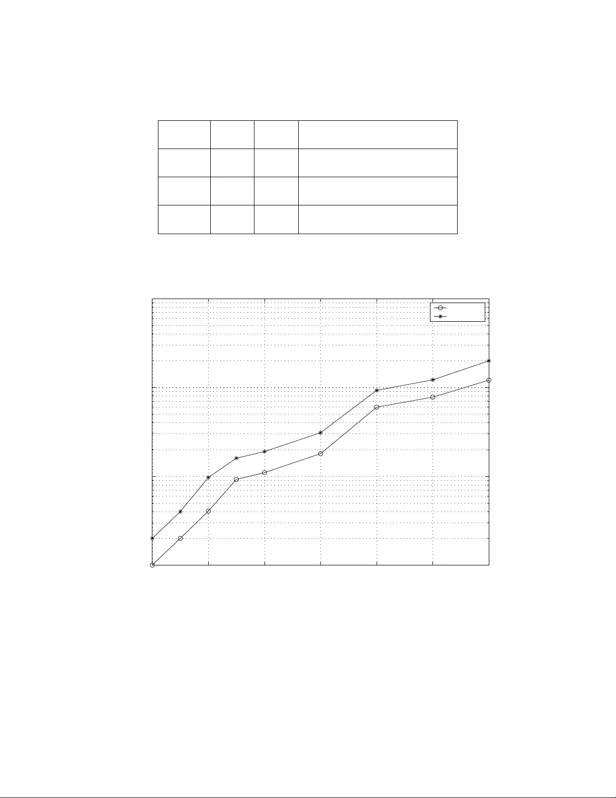
1 Deterministic Design of Low-Density Parity-Check Codes for Binary Erasure Channels 1 Hamid Saeedi and Amir H. Banihashem i Department of Systems and Computer Engineering Carleton University, Ottawa, Canada {hsaeedi,ahashmei@sce.carleton.ca} Abstract- We propose a deterministic method to design irregular Low -Density Parity-Check (LDPC) codes for binary erasure channels (BEC). Compared to the existing methods, which are based on the application of asymptomatic analysis tools such as density evolution or Extrinsic Information Transfer (EXIT) char ts in an optimization process, the proposed method is much simpler and faster. Through a number of examples, we demonstrate that the codes designed by the proposed method perform very cl osely to the best codes designed by optimization. An important property of the proposed designs is the flexibility to select the num ber of constituent varia ble node degrees P . The proposed designs include existing deterministic designs as a special case with P = N- 1, where N is the maximum variable node degree. Compared to the existing de terministic designs, for a given rate and a given δ > 0, the designed ensembles can have a threshold in δ -neighborhood of the capacity upper bound with smaller values of P and N . They can also achieve the capacity of the BEC as N , and correspondingly P and the maximum check node degree tend to infinity. Index Terms— channel coding, low-density parity-check (LDPC) codes, binary erasure channel (BEC), deterministic design. I. INTRDOUCTION Low-Density Parity-Check (LDPC) codes have rece ived m uch attention in the past decade due to their attractive performance/complexity tradeoff on a variety of comm unication ch anne ls. In particula r, on the Binary Erasure Channel (BEC), they achieve the ch annel capacity asymptotically [1-4]. In [1],[5],[6] a complete mathematical analys is for the performan ce of LDPC codes over the BEC, both asymptotically and for finite block lengths, has been developed. For other types of channels such as the Binary Symmetric Channel (BSC) and the Binary Input Additive W hite Gaussian Noise (BIAWGN) channel, only asymptotic analysis is available [7]. For irre gular LDPC codes, the problem of finding ensem ble 1 A preliminary versi on of this paper has been accepted fo r presentation at IEEE Globecom 2007, Washington D.C., USA, Nov. 26– 30, 20 07. 2 degree distributions (denoted by ρ ( x ) and λ ( x ) for check nodes and variable nodes, respectively) that perform well (i.e., have the best threshold for a given ra te or h ave the highest rate with neglig ible error or erasure probability for a give n channel parameter) is ca lled code design . For a variety of channels, the search for the best ensemble can be carried o ut base d on different asymptotic analysis tools such as density evolution and Extrinsic Information Transfer (EXIT) charts [8-10] through an optimization process. In [1], a linear programming approach base d on density evolution is used to find good degree distributions for the BEC. For the c ode design, there are two m ain cate gories in general: 1) For a given channel parameter, we look f or a code with maximum rate and negligible probability of error or erasure; 2) For a given rate, the code capable of providing a re liable transmissio n for the worst possible channel parameter is designed. The second category is of more pr actical interest, while the first category is usually easier to design. For a given set of constituent vari able an d check node degrees, and for a given BEC parameter ε (a given code rate R ), the ensem ble ( ρ ( x ) , λ ( x )) which provides the highest reliable transmission rate (highest er asure protection) is called the optimum ensemble. Optimization-based design methods are com putat ionally expensive especially when a large number of constituent variab le and check node degrees are permitted in the optimization proces s. In this paper, our aim is to deterministi cally design a close-to-optim um ense m ble for a given check node degree distribution and a given number P of constituent variable node degr ees. The designed ensembles are expected to perform closely to the best ensembles designed by optim ization. Fo r both categories of code design, we consider two cases: A) The case where al l the variable node degr ees from 2 to a maximum degree N are availa ble ( P = N -1); and B) the case where not all the degrees from 2 to N are used ( P ≠ N- 1). The ensembles designed in the two scenarios are referred to as Type-A and Type-B ensembles, respectively. In prac tice, the choice of P may be affected by implem entation considerations, where smaller values would be preferred. Although in this pa per we focus on the design of ensem bles for a given check node degree distribution, the designed ensembles can also be used to optim ize both the variable node and the check node degree distributions iterati vely in an optimization loop. In each iteration, ρ ( x ) and subsequently λ ( x ) (obtained by the method proposed in this pa per), is modified to optim ize the cost function (rate or threshold). In [2-4], the authors introduce sequences of degr ee distributions that asym ptotically achieve th e capacity of a BEC for large values of maximum variable and check node degrees. For finite values of maximum variable and check node degr ees, those sequences can also be us ed to deterministically design LDPC codes over a BEC. In fact, the constructions of [2-4] are a subset of constructions di scussed in this paper (Type A in Category 2 of code design). Here, we show that more favorable solutions for f inite values of P do exist in our extended family of designs, i. e., for a given rate, a given check node degree 3 distribution and a given δ > 0, the designed ensemble can have a threshold in δ -neighborhood of the capacity upper bound with a smaller value of P and a smaller m aximum vari able node degree, compared to the ensembles of [2-4]. It should be noted that although the sequences of [2-4] are special cases of the designs proposed in this paper, the approach taken here to derive them is different and much simpler than that of [2-4]. In addition, it can be proved that by a proper choice of P and for large values of N , the designed ensembles (in both categories and for both types) are capable of achieving the capacity of the BEC [11]. While this paper focuses on the code constr uction and simulation results for finite values of P and N , asymptotic results on the constructe d ensembles are presented in [ 11]. The paper is organized as follows. In the next section, we present a brief review of the BEC and its properties and define some notations that will be used throu ghout the paper. In section III, we discuss the first category of code design and prove a few lemmas that are used in the design process. Section IV generalizes the results of section III to the second categ ory of code design. In se ction V, we provide som e design examples. Section VI concludes the paper. The proofs of the lemm as, propositions and theorems are given in the appendix. II. PRELIMINARIES We represent an LDPC code ensemble with its variable node and check node degree distributions: 1 2 ) ( − = ∑ = i Dc i i x x ρ ρ and 1 2 ) ( − = ∑ = i D i i x x V λ λ , with constraints 1 2 = ∑ = Dc i i ρ and 1 2 = ∑ = V D i i λ , (1) where the coefficient of x i represents the percentage of edge s connected to the nodes of degree i+ 1, and D v and D c represent the maximum variable node de gree and the maximum check node degree, respectively. It should be noted that throughout the paper, we sometimes use N to represent the maxim um variable node degree. The difference between the two representations wi ll be clear from the context. Average check node and variab le node degrees are given by ∫ ∑ = = = 1 0 2 ) ( / 1 ) / /( 1 dx x i d Dc i i c ρ ρ and ∫ ∑ = = = 1 0 2 ) ( / 1 ) / /( 1 dx x i d V D i i v λ λ , respectively. For the code rate R , assuming a full-rank parity-check matrix, we have c v d d R / 1 − = . (2) 4 Consider a BEC with erasure probability ε . The capacity of this channel is C = 1 - ε . For a given code ensemble over a BEC with a given channel parameter ε , the sufficient and necessary condition for the zero probability of message erasure after in finite number of iterations of a simple erasure recovery algorithm [1] is x x < − − )) 1 ( 1 ( ρ ελ for x 0 ε ≤ < . This inequality can be rewritten as 0 ) 1 ( 1 ) ( 1 < − + − − x x ρ ελ , 1 x 0 ≤ < . (3) We call any code ensemble that s atisfies (3) convergent for the given ε . For a code ensemble, the threshold is defined as the supremum of all ε values that satisfy (3). III. CODE DESIGN FOR THE HIGHEST RATE In this section, we consider the case where we are given a check node degree distribution ρ ( x ) and a certain channel erasure probability ε . Our goal is to find the vari able node degree distribution λ ( x ) of a convergent ensemble with the largest rate. If N ( ≥ 3) denotes the maximum variable node degree, it is apparent from (2) that we need to minim ize the av erage variable node degree or maximize its inverse: i d N i i v / 2 1 ∑ = − = λ . (4) In fact, the optimization of the rate is equivalent to maxim i zing 1 − v d , subject to two constraints: equation (1) and inequality (3) which guaranties the code’s converg ence. From (4), it can be seen that in order to maxi mize 1 − v d , higher percentages have to be assigned to lower degree variable nodes. The following lemma is a formulation of this idea. Lemma 1 : Consider a given check node de gree distribution, a given channe l parameter and a given set of constituent variable node degrees. Let C be a convergent code ensemble of rate R with variable node degree distribution 1 2 ) ( − = ∑ = i N i i x x λ λ . For given integer numbers a and b in the inte rval [2 , N ], a ≠ b, we form a new ensemble C’ with rate R’ such that k a a − = λ λ ' , k b b + = λ λ ' and , ' i i λ λ = for { } b a i , ∉ ( k is chosen such that 0 ' ≥ a λ and 1 ' ≤ b λ ). We then have: 1) If a>b, then R R > ′ . 2) If a − = − ∑ ∞ = − − i i i i T x T x ρ . (5) By replacing (5) in (3), we obtain . 1 0 , 0 ) ( ... ) ( ) ( 1 1 1 2 3 3 2 2 ≤ < < − − + + − + − ∑ ∞ + = − − x x T x T x T x T N i i i N N N ελ ελ ελ (6) If x tends to zero, all the term s with powers greater than one can be ignored compared to the first term on the left hand side of (6). Therefore, as x tends to zero, we must have . ε λ ελ / 0 ) ( 2 2 2 2 T x T ≤ ⎯→ ⎯ ≤ − . (7) This is the upper bound on λ 2 . Note that ) 1 ( / 1 2 ρ ′ = T and thus (7) is the well-known stability condition 1 ) 1 ( 2 ≤ ′ ρ ελ [8]. Now suppose that we set λ 2 equal to the upper bound of (7). Then, the first term on the left hand side of (6) becomes zero. In this case, as x tends to 0, the term with x 2 becomes dominant and the necessary condition fo r convergence is ε λ ελ / 0 ) ( 3 3 2 3 3 T x T ≤ ⎯→ ⎯ ≤ − . We can continue in a similar fashion and obtain an upper bound on λ i , i.e. , ε λ / i i T ≤ , for 1 3 − ≤ ≤ N i , assuming that all λ j values for j = 2 ,..,i- 1, have their maxim um values. 2 1) Type-A Now assume that all variable node degrees from 2 to N are available. The above inequalities suggest that for a given ε and a given ρ ( x ), the following ensem ble, which is designed deterministically, could be a close-to-optimum candidate if it is convergent: 2 It should be noted that thi s result coi ncides with the flatness condi tion prop osed in [3] for capacity achievi ng sequenc es. Th e sequences of [3] however belon g to the seco nd category of code desig n. 6 ; 1 2 , / − ≤ ≤ = N i T i i ε λ ∑ − = − = 1 2 1 N i i N λ λ . (8) We show that for a given ρ ( x ) and a given ε , there exists a lower bound on N that will ensure the convergence and an upper bound which guarantees N λ to be positiv e. The following lemma indicates that a unique N satisfies both conditions. We call th e corresponding degree distributions Type-A . Theorem 1 : Consider a given check node degree distribution ρ ( x ) , and denote the i th term of the Taylo r expansion of ) 1 ( 1 x − − ρ at x = 0 by T i , as in (5). For a given channel param eter ε ≥ T 2 and a set of constituent variable node degrees from 2 to N ( N > 2), 3 there exists a unique N that satisfie s the following bounds: , 2 ε > ∑ = N i i T (9) ∑ − = ≥ 1 2 N i i T ε . (10) For such N, the convergence of Type-A ensemble is ensured and 0 ≥ N λ . Note that if we would like to design a code for a channel parameter ε which is less than T 2 , we have to decrease T 2 by increasing the average check node degree through the modification of ρ ( x ) . Theorem 2 : Consider the Type-A ens emble C designed based on (8) for a given channel param eter ε . The channel parameter ε is then the th reshold of C . W e note that for check-regular codes with the check node degree D c , there is a closed form expression for T i : () 1 1 i i T i α ⎛⎞ =− ⎜⎟ − ⎝⎠ , ) 1 ( 1 − = c D α , (11) where ⎟ ⎟ ⎠ ⎞ ⎜ ⎜ ⎝ ⎛ i α is defined as [2]: 3 Note that based on (8), th e condition 2 T ≥ ε is equivale nt to 1 2 ≤ λ . 7 () ( ) 1 1 1 2 1 .... 1 1 ! ) 1 )...( 1 ( + − − ⎟ ⎠ ⎞ ⎜ ⎝ ⎛ − ⎟ ⎠ ⎞ ⎜ ⎝ ⎛ − − = + − − = ⎟ ⎟ ⎠ ⎞ ⎜ ⎜ ⎝ ⎛ i i i i i i α α α α α α α α . (12) Example 1 : For ε = 0.48 and 5 ) ( x x = ρ , it can be seen th a t the value of N which sa tisfies (9) and (10) is N = 13. The variable node degree dist ribution for Type-A ensemble is: 12 11 10 9 8 7 6 5 4 3 2 0165 . 0 0204 . 0 0229 . 0 0260 . 0 0300 . 0 0353 . 0 0426 . 0 0532 . 0 0700 . 0 1000 . 0 1667 . 0 4167 . 0 ) ( x x x x x x x x x x x x x + + + + + + + + + + + = λ This ensemble has rate R = 0.4998 and its threshold is 0.48. Note that Type-A ensem bles are optimal in a gree dy sense, in that, starti ng f r om degree-2 variable nodes, we maximize the percentage of edges connected to lower degree variable nodes and thus aim for maximizing the rate of the ensem ble. For a fixed check degree distribution and a given channel parameter, however, the value of N and thus the number of constitue nt vari able node degrees are both f ixed and dictated by Theorem 1. In the fo llowing, we introduce new ensembles, where we have the flexibility to determine the number of consti tuent variable node degrees P and design ensembles with P < N -1. The cost associated with reducing P is a reduction in rate. 2) Type-B Given a check node degree distribution and a channe l parameter, Theorem 1 indicates that there exists a unique N that satisfies (9) and (10). For such N , consider a variable node degree distribution which includes a few consecutive de grees starting from 2 and ending at P − − = = ∑ ∑ and thus i T T d N i i N i i v / 2 2 1 ∑ ∑ = = − > . (17) Also, (10) should hold for the N th coefficient to be non-negative: i T T d N i i N i i v / 1 2 1 2 1 ∑ ∑ − = − = − ≤ . (18) 10 Theorem 3 : For a given code rate R and a given check node degree distribution (and thus a given 1 − v d ), if c d R / 2 1 − < , 4 then there exists a unique value of N that satisfies (17) and (18). Note that if the code rate R does not satisfy the inequality of Theorem 3, we would have to increase c d through modifying ρ ( x ). To summarize the design: For a given ra te and a given check node degr ee distribution, we first find T i values, then compute N from (17) and (18). Coefficients λ i are finally obtained b ased on (16). Note tha t with an argum ent similar to that of Theorem 2, one can show that the channel param eter obtained by (15) is in fact the true threshold of the Type-A ensemble. Example 4 : For R = 0.5 and 5 ) ( x x = ρ , it can be seen that the value of N which satisfies (17) and (18) is 13. The variable node degree distribut ion for the Type-A ensemble is . 0133 . 0 0204 . 0 0229 . 0 0260 . 0 0300 . 0 0353 . 0 0426 . 0 0532 . 0 0700 . 0 1000 . 0 1667 . 0 4169 . 0 ) ( 12 11 10 9 8 7 6 5 4 3 2 x x x x x x x x x x x x x + + + + + + + + + + + = λ This code has a threshold ε = 0.4798. 2) Type-B Similar to Type-B ensembles of s ubsection III.2, in this subsection, we consid er ensem bles with a few consecutive variable node degrees from 2 to P and a maxim um degree N . We initiate the de sign by computing N from (17) and (18) and then com puting ε from the following equation: N d R N i T c P i i / 1 ) 1 ( ) / 1 / 1 ( 1 1 2 − − − = − − = ∑ ε . (19) We then set /, 2 ii Ti P λ ε =≤ ≤ , and ∑ = − = P i i N 2 1 λ λ . (20) Theorem 4 : Coefficient λ N in (20) is positive. In the following theorem, we also show that the new ensemble is convergent. Theorem 5 : A Type-B ensemble of rate R is convergent over a channel w ith parameter equal to the value given in (19). Moreover this value is the threshold of Type-B ensemble. 4 Note that this inequality is satisfied for any ensemble whose variable node degrees are at least two. 11 Similar to the case in subsection III.2, to obtain a better threshold for a given P , we can design a Type-MB ensemble by decreasing the maximum variable node degree from N to a smaller va lue D v . To design this ensemble, we use (19) and (20) with N replaced by D v , and find the smallest D v for which the ensemble is convergent for the channel parameter gi ven by (19). W ith a simila r argument used for Type- A and B ensembles, the value of (19) is the threshold of the Type-MB ensem ble. Unfortunately, for this category of code design, we ha ve not been ab le to obtain a lower bound for D v similar to that of Proposition 1. One however can perform a maximum of N-P trials to find the smallest D v . Each trial consists of computing ε from (19) and λ ( x ) from (20), where in both equations N is replaced by D v . We then need to check whether in equ ality (3) holds for the tested D v . Example 5: Consider the Type-B ensem ble with P = 4 and D c = 6 corresponding to the Type-A ensemble of Example 4. This ensemble has variable node degrees 2, 3, 4 and 13, with coefficients λ 2 = 0.4521, λ 3 = 0.1808, λ 4 = 0.1085 and λ 13 = 0.2586, respectively. The threshold of this ensemble computed by (19) is ε = 0.4424, which is less than that of the Type-A ensemble of Exam ple 4, as expected. If we keep decreasing the maximum variable node degree, we see th at a degree distri bution with degrees 2, 3, 4 and 8 is convergent while one with 2, 3, 4 and 7 is not. Therefore, for R = 0.5 and 5 ) ( x x = ρ , Type-MB ensemble has variable node degrees 2, 3, 4 and 8 with coefficients λ 2 = 0.4266, λ 3 = 0.1706, λ 4 = 0.1024 and λ 8 = 0.3004. This ensemble has a threshold ε = 0.4688, obtained from (19), which is in betw een the thresholds of Type-A and Type-B ensembles, and quite close to th at of Type-A ensemble. It is how ever important to note that compared to Type-A ensemble, which has 12 different variable node degrees with a maximum degree of 13, this ensemble has on ly 4 different variable node degrees and the m aximum degree is only 8. V. SIMULATION RESULTS For simulation results, we consid er both categories of code de sign for the highly popular check- regular ensembles 5 . We first consider an upper bound from [2] which is useful to m easure the performance of our designed ensembles: For a given rate R and a given averag e check node degree c d , the best achievable thres hold is upper bounded by З ) 1 )( 1 ( c d R R − − = . By modifying the upper bound of [2], for a given channel parameter ε and a given c d , we obtain the following upper bound on th e best achievable rate: Я ) ) 1 ( 1 ( 1 c d ε ε − − − = . 5 The popularity of check-regu lar ensem bles is due to thei r better erasure correcting capabilities and si mpler implementation in hardware. For a reference on the former, see [4]. 12 Example 6 : Consider the second category of code design for rate one half. Suppose that there is a constraint of P = 4 on the num ber of different variable node degrees. We consider check-regular ensembles with D c = 5, 6, and 7. Table I shows the designed Type-MB ensembles for each check node degree. Note that for R = 0.5 , the capacity upper bound implies ε < 1 -R = 0.5. For each ensem ble, we have shown the ratio of the threshold to 1 -R = 0.5 as well as to З . As can be seen, the thre shold im proves by increasing D c and the ensemble with check node degree 7 achieves close to %97 of the upper bound З . In fact for P = 4, this is the best threshold than can be obtained by Type-MB check-regular ensembles. By increasing D c further, the threshold decreases unless we allow P to also increase. Example 7: In this example, by still focusing on check-regular ensembles, we allow P to take values between 5 and 10 and for each value of P , we find the value of D c which results in the best thres hold for Type-MB ensembles. These results are reported in Tabl e II. As can be seen the threshold improves as P is increased. Example 8: In this example, we compare the perf ormance of the Type-MB ensemble with D c = 7 and P = 8 designed in Example 7 with its corresponding Type-A ensemble with the same check node degree distribution. The Type-A ensemble has the fo llowing variable node de gree distribution: . 0025 . 0065 . 0067 . 0071 . 0074 . 0078 . 0082 . 0087 . 0092 . 0097 . 0104 . 0111 . 0119 . 0128 . 0139 . 0152 . 0167 . 0185 . 0207 . 0234 . 0269 . 0315 . 0378 . 0469 . 0612 . 0864 . 1414 . 3394 . ) ( 28 27 26 25 24 23 22 21 20 19 18 17 16 15 14 13 12 11 10 9 8 7 6 5 4 3 2 x x x x x x x x x x x x x x x x x x x x x x x x x x x x x + + + + + + + + + + + + + + + + + + + + + + + + + + + = λ The threshold of this ensemble is equal to 0.4910 whic h is slightly better than that of Type-MB ensem ble (0.4891). This is at the expense of 28 different variable node degrees (i nstead of 8 for Type-MB) and the maximum variable node degree of 29 (instead of 15 fo r Type-MB). In Fig. 1, we have shown the finite block length simulation results fo r the two codes. The block length is selected to be 5000 and the maximum number of iterations is lim ited to 2 00. For each simulation poi nt, one hundred codeword erasures are generated. As can be seen, the two c odes perform closely in fi nite block length as well. In the next example, we demonstrate that fo r large enough m aximum va riable and check node degrees and P , Type-MB ensembles can practically achieve the cap ac ity sim ilar to the sequences of [2-4]. Example 9: We consider again rate one-half check-regular ensembles. W ith D c = 11 and P = 90, we obtain D v = 203 for a Type-MB ensemble. The threshold for this ensemble is equal to 0.4993 which is %99.9 of the capacity upper bound . If we use the check reg ular sequences of [4] with D c = 11, to achieve the same percentage of the capacity bound , the designed code has to have 522 different constitu ent variable node degrees. Also, the maximum va riable node degree increases from 203 to 523. 13 In the following, we compar e our resu lts with those obtained by op timization. Example 10: From the database [12] of optimized LDPC co des, we consider the following check-regular rate one-half ( R = 0.5) ensemble C 1 with D c = 7: 15 14 5 4 3 2 1126 . 0 1305 . 0 1620 . 0 0783 . 0 0095 . 0 1716 . 0 3354 . 0 ) ( 1 x x x x x x x x C + + + + + + = λ . For this ensemble, P = 7 and the threshold 1 C ε is equal to 0.4917. For P = 7 and D c = 7, the Type-MB ensemble C 2 has D v = 14 with the following variab le node degree distribution: 13 6 5 4 3 2 2824 . 0 0380 . 0 0472 . 0 0616 . 0 0870 . 0 1423 . 0 3415 . 0 ) ( 2 x x x x x x x x C + + + + + + = λ . This ensemble has a threshold 2 C ε = 0.4880 which is only slightly less than that of C 1 . It should however be noted that the maximum variable node degree for C 2 (14) is smaller than that of C 1 (16). If we restrict the maximum variable node degree to 14 or sm aller, we find another optimized ensemble C 3 in [12] with the following variab le n ode degree distribution: 12 3 2 2848 . 0 1162 . 0 3135 . 0 2853 . 0 ) ( 3 x x x x x C + + + = λ . Incidentally, this ensemble has the same threshold of 0.4880 as C 2 does. The advantage of this ensemble over C 2 is however the fewer number of constituent variable node degrees and the m aximum variable node degree of 13 instead of 14. Example 11: In this example, we consider the first category of code design. Let D c = 5, ε = 0.48, and consider a constraint of P = 4 on the number of different variable node degrees. Using (9) and (10), we obtain N = 7. If we limit our search fo r an optimal ensemble to the maximum variable node degree of 7, there are a total of ⎟ ⎟ ⎠ ⎞ ⎜ ⎜ ⎝ ⎛ 4 6 = 15 different sets of constituent vari able node degrees to be tested. We have performed optimization using exhau stive search for each set of constituent variable node degrees. Some of the best results are given in Table III. No te that for each row of Table III, the best ) ( x λ which maximizes the rate for a convergent ensemb le has been obtained. The highest ratio R / Я in the table is 0.9624, which corresponds to achieving about %96 of the rate upper bound. Using our design method, we obtain a Type-MB en semble with the following variable node degree distribution: 5 3 2 1699 . 0 1139 . 0 1953 . 0 5208 . 0 ) ( x x x x x + + + = λ . The rate of this ensemble is 0.4769 which is more than %95 of the upperbound Я . This is only slightly worse than the best result f rom the exhaustive search. The com plexity of our design however is substantially lower than that of the ex haustive search. 14 VI. CONCLUSIONS In this paper, we propose methods to deterministic ally design ensembles of irregular LDPC codes for binary erasure channels. The main idea is to m a ximize the percen tage of edges connected to lower degree nodes in a greedy fashion. At finite maxim um variable a nd check node degrees, the designed ensembles perform close to optimal, onl y slightly inferio r to the ensemb les designed by exhaustive search (or optimization algo rithms with asymptotic ana lysis tools). This is while the design com plexity of the proposed ensembles is substantially lower th an those obtained by e xhaustive search. An important feature of the propose d design is th e flexibility to choose the number of constituent variable node degrees P , and to de terministically design a c lose to optim al ensemble under th is constraint. Check-regular ensembles designed by this method woul d provide attractive soluti ons for im plementation. The proposed ensembles are also capable of achieving the capacity as th e maximum variable and check node degrees increase. While capacity-achieving ensembles of [4] are spec ial cases of the proposed designs, the derivation approach in this paper is different and much simpler. Moreover, our extended family of designs inclu de more attractiv e solutions for finite values of P , i.e., for a given rate, a given check node degree dist ribution and a given δ > 0, the designed ensembles can have a threshold in δ - neighborhood of the capacity upper bound with a smaller value of P and a sm aller maximum variab le node degree, compared to the ensembles of [4]. A topic of future research would be to obtain similar results on de terministic design s of irregular LDPC code ensembles for other cha nnels such as the AW GN channel. Appendix: Proof of the Lemmas, Propositions and Theorems Proof of Lemma 1: To prove claim 1, we show that v v d d / 1 / 1 > ′ : v b a D b a i i i b a D b a i i i v d b a i b k a k i d V V / 1 / / / / ) ( / ) ( / / 1 , , 2 , , 2 = + + > + + − + = ′ ∑ ∑ ≠ = ≠ = λ λ λ λ λ λ , where the inequality follow s from b a > . For claim 2, we show that the degree di stribution for C’ satisfies (3). Fo r 0 < x ≤ 1, b a < , and k ≥ 0 , it is easy to see that k.x b- 1 -k.x a- 1 ≤ 0 . As a result, for 0< x ≤ 1, λ a x a- 1 + λ b x b -1 ≥ ( λ a -k ) x a- 1 + ( λ b +k ) x b- 1 = λ ’ a x a- 1 + λ ’ b x b- 1 , and therefore λ ( x ) ≥ λ ’ ( x ). This im plies that if λ ( x ) satisfies (3), so does λ ’ ( x ) , and thus C’ is convergent. 15 Proof of Theorem 1 : From (5), we have 2 1 i i T ∞ = = ∑ , and since T 2 ≤ ε < 1, and i T i ∀ > , 0 , it is easy to see th at there ex ists an integer N that satisfies both (9) and (10) and that such N is unique. For such N , to show the con vergence of the Type-A ensemble, we verify (3). Substituting 1 2 , / − ≤ ≤ = N i T i i ε λ in (3), we obtain: 1 0 , 0 ) ( 1 1 1 ≤ < < − − ∑ ∞ + = − − x x T x T N i i i N N N ελ . To show that the above inequality ho lds, we note that ∑ − = − = 1 2 N i i N T ε ελ , and thus ∑ = < − = − N i i N N T T 2 0 ε ελ , where the last inequality is the sam e as (9). Multiplying both sides by the positive value x N-1 , and subsequently subtracting the positive value of ∑ ∞ + = − 1 1 N i i i x T from the left hand side proves (3) and thus the convergence. To prove that N λ is nonnegative, we divide both sides of (10) by ε , and obtain ∑ − = ≤ 1 2 1 N i i λ , which implies 0 ≥ N λ . Proof of Theorem 2 : To prove that the channel param eter ε is the threshold of the Type-A ensemble C , we show th at if C converges over a channel with parameter ε ’ , we must have ε ≥ ε ’ . Based on (7), channel parameter ε ’ mus t satisfy ' / 2 2 ε λ T ≤ . By the construction of C , however, ε λ / 2 2 T = , and therefore ' / / 2 2 ε ε T T ≤ . This requires that ' ε ε ≥ . Proof of Proposition 1 : We denote the variable node de gree distribution for ensemble C with λ ( x ). For the given check node degree distribution and channel paramete r, we construct the Type-A ensemble C’ and denote its variable node degree distribution by λ ’ ( x ). Th e maxi mum var iabl e node degree for ensemble C’ is N . If 1 − = v D P , then C will be the same as Type-A ensemble C’ , and the proposition is triv ial. We thus focus on 1 − < v D P . First note that based on (3), we have 1 0 ), 1 ( 1 ) ( ' 1 ≤ < − − < − x x x ρ ελ . (A-1) 16 We define function f as follows: 1 2 2 1 1 1 2 1 2 1 ) ( ) ( ) ( ) ( ' ) ( − = = − − − = − = − ∑ ∑ ∑ ∑ − − − − + = − = Dv P i i P i i i N N i i N i i i x T x T x T x T x x x f ε ε ελ ελ , We therefore have 1 1 2 1 2 1 1 1 ) ( ) ( ) ( − − = − = − + = − ∑ ∑ ∑ − + − − = N N i i Dv P i i N P i i i x T x T x T x f ε ε . We now consider two cases: a) N D v = and b) N D v < , and for both cases prove that ) ( x f is strictly positive over the interv al (0, 1). For case (a), co mbining the last two terms of ) ( x f results in ∑ − + = − − 1 1 1 ) ( N P i N i x T . It is then easy to see that ) ( x f has only one sign change between consecutive nonzero coefficients. Based on Descartes’ rule of signs, this implies that ) ( x f has only one positive root. It is easy to see 0 ) 1 ( = f , and thus x = 1 is the only positive root of ) ( x f . We also have 0 ) 0 ( = f , and therefore ) ( x f must be either strictly positive or strictly negative in the in terval (0, 1). Using (13), it is a sim ple exercise to see 0 ) 1 ( ' < f , and thus ) ( x f must be strictly positive over (0, 1). For case (b), ) ( x f has two sign changes between consecutive nonzero coefficients. Based on Desc artes’ rule o f signs, this implies tha t ) ( x f has either zero or two positive roots. Since 0 ) 1 ( = f , we must have the latter case. It is also easy to see that 0 ) 1 ( ' < f . This combined with +∞ = +∞ → ) ( lim x f x indicates that the othe r positive root of ) ( x f mu st be larger than one, and thus ) ( x f does not have any root in (0, 1). It therefore m ust be either strictly positive or strictly negative in the interval. Since 0 ) 1 ( ' < f , it must be the form er. Since ) ( x f is strictly positive over (0, 1), we have ) ( ' ) ( x x ελ ελ < for 0< x <1. This combined with (A-1) proves that ensemble C is convergent. Proof of Theorem 3: Since R > 0, we have c v d d < , and thus 1 1 0 ) ( − < ∫ v d dx x ρ . Since for 0 < x < 1 , 0 < ρ ( x ) < 1, one can easily s ee that dx x dx x ∫ ∫ − − = 1 0 1 1 0 ) ( 1 ) ( ρ ρ . We therefore have 17 1 1 0 1 0 1 1 0 1 ) ( ) ( 1 ) 1 ( 1 − − − < = − = − − ∫ ∫ ∫ v d dx x dx x dx x ρ ρ ρ . (A-2) Consider the following sequences for n ≥ 2 : i T n g T d n f n i i n i i v / ) ( ) ( 2 2 1 ∑ ∑ = = − = = To prove Theorem 3, we prove that there exists a unique N that satisfies ) ( ) ( N g N f > and ) 1 ( ) 1 ( − ≤ − N g N f . Both sequences f and g are strictly increasing. We note that based on inequality c d R / 2 1 − < , we have 2 / 1 1 < − v d . Also, 2 1 ) 2 ( T d f v − = and 2 / ) 2 ( 2 T g = . We thus have ) 2 ( ) 2 ( g f < . Moreover, we have 1 1 2 1 2 1 ) ( = − = − = − ∑ ∑ = = x i n i i v n i i v x T d T d n f and 1 2 2 / ) ( / ) ( = = = ∑ ∑ = = x i n i i n i i i x T i T n g . Based on (5), this results in 1 1 1 1 )) 1 ( 1 ( ) ( lim − = − − ∞ → = − − = v x v n d x d n f ρ , and 1 1 0 1 1 0 1 ) 1 ( 1 ) 1 ( 1 ) ( lim − − − ∞ → < − − = − − = ∫ ∫ v n d dx x dx x n g ρ ρ , where the last inequality is based on (A-2). W e thus have ) ( lim ) ( lim n g n f n n ∞ → ∞ → > . Putting this together with ) 2 ( ) 2 ( g f < , we conclude that there exist som e finite n>2, for which ) ( ) ( n g n f > . Let N be the smallest such n . We thus have 1 2 ), ( ) ( − ≤ ≤ ≤ N n n g n f . (A-3) It is also easy to see that N satisfies N d v / 1 1 > − , (A-4) because otherwise, we have N i i T N T T d i i i v ≤ ≤ ≤ ≤ − 2 for , / / 1 , and therefore 18 i T T d N i i N i i v / 2 2 1 ∑ ∑ = = − ≤ . (A-5) This means that f ( N ) ≤ g ( N ), which contradicts the above definition of N . Now we prove that for any n>N , f ( n ) >g ( n ). Using (A-4), we have , / / 1 i T N T T d i i i v > > − for i > N , and thus for any n>N , we have i T T d n N i i n N i i v / 1 1 1 ∑ ∑ + = + = − > . (A-6) This together with f ( N ) >g ( N ) results in i T T d n i i n i i v / 2 2 1 ∑ ∑ = = − > , (A-7) which is equivalent to f ( n ) >g ( n ) . This proves the uniqueness of N . Proof of Theorem 4 : Note that based on the proof Theorem 3, the value of N that satisfies (17 ) and ( 18) is unique and using (A- 3), for any P N λ . Proof of Theorem 5 : Let C denote the Type-B ensemble. For the given check node degree distribu tion a nd code rate, let C’ denote the corresponding Type -A ensemble. Note that C’ is convergent on a channel with parameter equal to (15). Denote the threshold of ensemble C ’ by ε ’ . We have ∑ ∑ = − = − − + = P i N i P i i i x T x T x 2 1 2 1 ) / 1 ( ) / ( ) ( ε ε λ , and 19 ∑ ∑ − = − − = − − + = 1 2 1 1 2 1 ) ' / 1 ( ) ' / ( ) ( ' N i N i N i i i x T x T x ε ε λ . Therefore ∑ ∑ = − = − − + = P i N i P i i i x T x T x 2 1 2 1 ) ( ) ( ε ελ , (A-9) and ∑ ∑ − = − − = − − + = 1 2 1 1 2 1 ) ' ( ) ( ' ' N i N i N i i i x T x T x ε λ ε . (A-10) Ensemble C’ is convergent by de finition, therefore 1 0 for ), 1 ( 1 ) ( ' ' 1 ≤ < − − < − x x x ρ λ ε . (A-11) We also have ' / 1 ) 1 ( ) / 1 / 1 ( / 1 ) 1 ( ) / 1 / 1 ( 1 1 1 2 1 1 2 ε ε = − − − < − − − = − − − = − − = ∑ ∑ N d R N i T N d R N i T c N i i c P i i , since P < N -1 for Type-B ensemble, and 1/ i > 1/ N for i ≤ N -1. Therefore ε < ε ’ , and consequently ∑ ∑ ∑ ∑ − = − − = − − = − − = − − + < − + 1 2 1 1 2 1 1 2 1 1 2 1 ) ' ( ) ( N i N i N i i i N i N i N i i i x T x T x T x T ε ε . (A-12) Also, as 1 0 ≤ < x , one can see that 0 1 1 ≥ − − − N i i i x T x T , for 1 1 − ≤ ≤ + N i P , and thus 0 1 1 1 1 1 1 ≥ − ∑∑ − + = − + = − − N P i N P i N i i i x T x T . (A-13) Adding (A-13) to (A -9), we obtain ∑ ∑ − = − − = − − + ≤ 1 2 1 1 2 1 ) ( ) ( N i N i N i i i x T x T x ε ελ . (A-14) Combining (A-14), (A-12) and (A-10), we have ) ( ' ' ) ' ( ) ( ) ( 1 2 1 1 2 1 1 2 1 1 2 1 x x T x T x T x T x N i N i N i i i N i N i N i i i λ ε ε ε ελ = − + < − + ≤ ∑ ∑ ∑ ∑ − = − − = − − = − − = − , and thus ) ( ' ' ) ( x x λ ε ελ < . (A-15) From (A-11) and (A-15) we conclude that 1 0 for ), 1 ( 1 ) ( 1 ≤ < − − < − x x x ρ ελ , 20 which proves the convergence. With an argument sim ilar to that of Theorem 2, one can show that (19) is in fact the threshold of the Type-B ensem ble. REFERENCES [1] M.G. Luby, M. Mitzenmacher, M.A. Shokrollahi, and D.A. Spielman, “Effic ient erasure correcting codes,” IEEE Trans. Inform. Theory , vol. 47, no. 2, pp. 569-584, Feb 2001. [2] A Shokrollahi, ”New sequences of linear time eras ure codes approaching the channel capacity,” in proc . 13th Int. Symp. on Applied Algebra, Alge braic Algorithms, and Error Correcting Codes ( M. Fossorier, H. Imai, S. Lin, and A. Poli ), no. 1719 in Lecture Notes in Computer Science, 1999, pp. 65-76. [3] A. Shokrollahi, “Capaci ty-achieving sequences,” in Codes, Systems, and Graphical Models (IMA Volumes in Mathematic s and Its Applications ), B. Marcus and J. Rosenthal, Eds. New York: Springer- Verlag, 2000, vol. 123, pp. 153–166. [4] P. Oswald and A. Shokrollahi, “Capacity-A chieving Sequences for the Erasure Channel,” IEEE Trans. Inform. Theory, vol. 48, no. 12, pp. 3017-3028, Dec. 2002. [5] C. Di, D. Proietti, I.E. Telatar, T.J. Richard son, R.L. Urbanke, “Finite-length analysis of low-density parity-check codes on the binary erasure channel,” IEEE Trans. Inform. Theory , vol. 48, no. 6, pp. 1570 – 1579, June 2002 . [6] T. Richrdson, A. Shokrollahi, and R. Urbanke, “Finite-length analysis of various low-density parity- check ensembles for the binary erasure channel,” in Proc. IEEE Int. Symp. Inform. Theory, Switzerland, July 2002 , p. 1. [7] T. J. Richardson and R. L. Urbanke, “The capaci ty of low-density parity-check codes under message- passing decoding,” IEEE Trans. Inform. Theory , vol. 47, pp. 599-618, Feb. 2001. [8] T. J. Richardson, A. Shokrolla hi, and R. L. Urbanke, “Design of capacity ap proaching irregular low density parity check codes,” IEEE Trans. Inform. Theory , vol. 47, no. 2, pp. 619–637, Feb. 2001. [9] S. Y. Chung, T.J. Richardson, and R. L. Urbanke, “Analysis of sum-product decoding of LDPC codes using a Gaussian approximation,” IEEE Trans. Inform. Theory , vol. 47, no. 2, pp. 657-670, Feb. 2001. [10] S. ten Brink, G. Kramer, and A. Ashikhmin, “Design of lo w-density parity check codes for modulation and detection,” IEEE Trans. Comm., vol. 52, no. 4, pp. 670-678, April 2004. [11] H. Saeedi and A. H. Banihash emi, “New Sequences of Capacity-A chieving Sequences for the Binary Erasure Channel,” to be submitted to IEEE Trans. Inform. Theory, Sept. 2007. [12] R. Urbanke. Report. [O nline]. Available: http://lthcwww.epfl.ch/research/ldpcopt/ 21 Table I: Type-MB ensembles for R = 0.5 and P = 4 . D c D v ε MB/ 0.5 ε MB / З λ ( x ) 5 6 0.8873 0.9159 5 3 2 1019 1233 . 2113 . 5635 . x x x x + + + 6 8 0.9376 0.9525 7 3 2 3004 . 1024 . 1706 . 4266 . x x x x + + + 7 10 0.9610 0.9686 9 3 2 4203 . 883 . 1445 . 3459 . x x x x + + + Table II: Best Type-MB check-regular ensembles for R = 0.5 and different values of P . P D c D v ε MB /0.5 ε MB / З λ ( x ) 5 7 12 0.9624 0.9700 11 4 3 2 3586 . 0625 . 0882 . 1443 . 3464 . x x x x x + + + + 6 7 13 0.9716 0.9793 12 5 4 3 2 3173 . 0474 . 0619 . 0874 . 1429 . 3431 . x x x x x x + + + + + 7 7 14 0.9761 0.9838 13 6 5 4 3 2 2824 . 0380 . 0472 . 0616 . 0870 . 1423 . 3415 . x x x x x x x + + + + + + 8 7 15 0.9783 0.9860 14 7 6 5 4 3 2 2523 . 0316 . 0380 . 0471 . 0615 . 0868 . 1420 . 3407 . x x x x x x x x + + + + + + + 9 8 22 0.9836 0.9875 21 8 7 6 5 4 3 2 3225 . 0247 . 0288 . 0344 . 0425 . 0550 . 0771 . 1245 . 2905 . x x x x x x x x x + + + + + + + + 10 8 23 0.9864 0.9902 22 9 8 7 6 5 4 3 2 3031 . 0215 . 0246 . 0287 . 0343 0423 . 0549 . 0768 . 1241 . 2897 . x x x x x x x x x x + + + + + + + + + 22 Table III: Results for rate optimizati on of LDPC code ensembles with D c = 5 and 4 different constituent variable node degrees at channel erasure probability 0. 48. Variable node degrees R R/ Я λ ( x ) [2,3,4,6] 0.4821 0.9622 5 3 2 0005 . 4059 . 0730 . 5206 . x x x x + + + [2,3,4,5] 0.4822 0.9624 4 3 2 0682 . 0 2950 . 1172 . 5196 . x x x x + + + [2,4,5,6] 0.4739 0.9455 3 4792 . 5208 . x x + 0.46 0.47 0.48 0.49 0.5 0.51 0.52 10 −4 10 −3 10 −2 10 −1 Channel Erasure Probabilty Bit Erasure Rate Type A Type MB Figure 1: The performance of codes with bloc k length 5000 from the ensembles of Exam ple 8.