Theoretical analysis of optimization problems - Some properties of random k-SAT and k-XORSAT

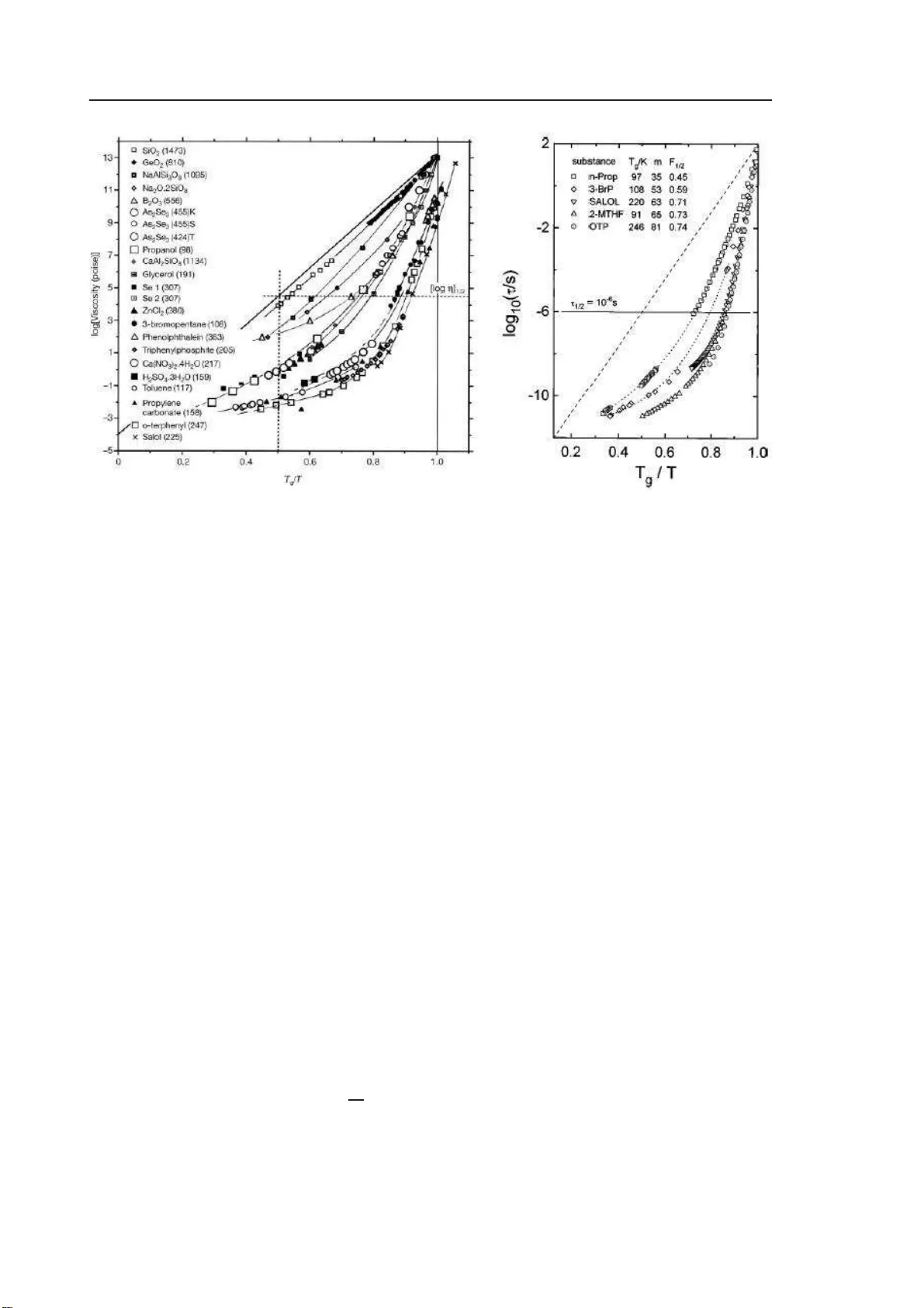
Sapienza Universit ` a di Roma Dottora to di Ricer ca in Fisica Scuola di dottora to “Vito Vol terra ” Theoretical analysis of optimization problems Thesis submitted to obt ain the degree of ”Dottor e di Ric er c a” - Do ctor Philosophiæ PhD in Physics - XX cycle - October 2007 by F abrizio Altarelli Program Co ordinator Thesis Advisors Prof. Enzo Marinari Prof. Giorgio P arisi Dr. Nicolas Sourlas Dr. R ´ emi Monasson Al la dottor essa F e derici Con ten ts In tro duction vii I Statistical mec hanics of optimization problems 1 1 Statistical mec hanics of disordered systems 3 1.1 Statistical mec hanics and phase transitions . . . . . . . . . . . . . . . . . . . . . . . . 3 1.1.1 The Gibbs distribution . . . . . . . . . . . . . . . . . . . . . . . . . . . . . . . . 3 1.1.2 Phase transitions and ergo dicity breaking . . . . . . . . . . . . . . . . . . . . . 5 1.2 Disordered sys tems and spin glasses . . . . . . . . . . . . . . . . . . . . . . . . . . . . 6 1.2.1 Origins of disor der . . . . . . . . . . . . . . . . . . . . . . . . . . . . . . . . . . 6 1.2.2 Spin g la ss mo dels . . . . . . . . . . . . . . . . . . . . . . . . . . . . . . . . . . . 7 1.2.3 Mean ﬁeld theo r y and diluted mo dels . . . . . . . . . . . . . . . . . . . . . . . 8 1.2.4 F rustra tion, lo c a l degeneracies, co mplexit y . . . . . . . . . . . . . . . . . . . . . 8 1.2.5 The o rder parameter of disor dered sy stems . . . . . . . . . . . . . . . . . . . . 9 1.3 Phenomenolog y of disordered sy stems . . . . . . . . . . . . . . . . . . . . . . . . . . . 10 1.3.1 Spin g la ss susceptibilities . . . . . . . . . . . . . . . . . . . . . . . . . . . . . . 10 1.3.2 Div erg ence of relax ation times . . . . . . . . . . . . . . . . . . . . . . . . . . . 12 1.3.3 Ageing . . . . . . . . . . . . . . . . . . . . . . . . . . . . . . . . . . . . . . . . . 13 1.4 The replica metho d . . . . . . . . . . . . . . . . . . . . . . . . . . . . . . . . . . . . . . 13 1.4.1 The r eplica trick . . . . . . . . . . . . . . . . . . . . . . . . . . . . . . . . . . . 13 1.4.2 Solution of the p -spin spherical mo del . . . . . . . . . . . . . . . . . . . . . . . 14 1.4.3 Replica formalism fo r diluted mo dels . . . . . . . . . . . . . . . . . . . . . . . . 17 2 Optimization problems and alg orithms 21 2.1 Some exa mples o f combinatorial o ptimization problems . . . . . . . . . . . . . . . . . 21 2.2 Bo olean satisﬁability: k - sa t and k - xorsa t . . . . . . . . . . . . . . . . . . . . . . . . 23 2.2.1 Int ro duction to k - sa t . . . . . . . . . . . . . . . . . . . . . . . . . . . . . . . . 23 2.2.2 Int ro duction to k - xorsa t . . . . . . . . . . . . . . . . . . . . . . . . . . . . . . 26 2.3 Computational complexity . . . . . . . . . . . . . . . . . . . . . . . . . . . . . . . . . . 26 2.3.1 Algorithms a nd computational resourc es . . . . . . . . . . . . . . . . . . . . . . 27 2.3.2 Computation mo dels and complexity cla sses . . . . . . . . . . . . . . . . . . . . 27 2.3.3 Reductions, hardness and completeness . . . . . . . . . . . . . . . . . . . . . . 30 2.3.4 Other mea sures of co mplexit y . . . . . . . . . . . . . . . . . . . . . . . . . . . . 31 2.3.5 Connections to the work presented in Part I I . . . . . . . . . . . . . . . . . . . 33 2.4 Search a lg orithms . . . . . . . . . . . . . . . . . . . . . . . . . . . . . . . . . . . . . . . 33 iii 2.4.1 Random-walk algor ithms . . . . . . . . . . . . . . . . . . . . . . . . . . . . . . 34 2.4.2 DPLL algorithms . . . . . . . . . . . . . . . . . . . . . . . . . . . . . . . . . . . 36 3 Phase transi tions i n random optimi za tion problems 43 3.1 Evidence o f phase tr ansitions from numerical ex periments . . . . . . . . . . . . . . . . 43 3.2 Rigorous der iv a tion of the phase diagra m o f k - xorsa t . . . . . . . . . . . . . . . . . . 44 3.2.1 Bounds from ﬁrs t and seco nd momen ts . . . . . . . . . . . . . . . . . . . . . . 4 5 3.2.2 Leaf remov a l pro cedure . . . . . . . . . . . . . . . . . . . . . . . . . . . . . . . 47 3.2.3 Phas e dia gram of k - xorsa t . . . . . . . . . . . . . . . . . . . . . . . . . . . . . 51 3.3 Heuristic results o n the phase diagra m of k - sa t . . . . . . . . . . . . . . . . . . . . . . 52 I I Some propert ies of random k -SA T and random k -XORSA T 55 4 Study of p oisso nian heuri s tics for DPLL in k -X ORSA T 57 4.1 Leaf-remov al for mixed for m ulæ . . . . . . . . . . . . . . . . . . . . . . . . . . . . . . . 58 4.1.1 Leaf-r emo v al diﬀerential equations . . . . . . . . . . . . . . . . . . . . . . . . . 58 4.1.2 Solution for c j ( t ) . . . . . . . . . . . . . . . . . . . . . . . . . . . . . . . . . . . 59 4.1.3 Solution for n ℓ ( t ) . . . . . . . . . . . . . . . . . . . . . . . . . . . . . . . . . . . 60 4.2 Character iz a tion of the pha s es in ter ms of a p otent ial . . . . . . . . . . . . . . . . . . 61 4.2.1 Deﬁnition and prop erties of the p oten tial V ( b ) . . . . . . . . . . . . . . . . . . 61 4.2.2 Phas e dia gram for mixed k - x orsa t formulæ . . . . . . . . . . . . . . . . . . . 63 4.3 T ra jectories gener ated by p oissonian heuris tics . . . . . . . . . . . . . . . . . . . . . . 64 4.3.1 Poissonian heuristics for DPLL . . . . . . . . . . . . . . . . . . . . . . . . . . . 65 4.3.2 Genera l prop erties of po issonian heuristics . . . . . . . . . . . . . . . . . . . . . 67 4.3.3 Analysis of UC a nd GUC . . . . . . . . . . . . . . . . . . . . . . . . . . . . . . 71 4.4 Bounds o n the v alues of α for which po issonian heuristics can succ eed . . . . . . . . . 73 4.5 Optimality of GUC for large k . . . . . . . . . . . . . . . . . . . . . . . . . . . . . . . 74 4.6 Conclusions and p ersp ectiv e s . . . . . . . . . . . . . . . . . . . . . . . . . . . . . . . . 76 5 Characterization of the sol utions of k -SA T at large α 79 5.1 Problem deﬁnition a nd pr eviously established results . . . . . . . . . . . . . . . . . . . 80 5.1.1 Deﬁnition of the r a ndom ensembles . . . . . . . . . . . . . . . . . . . . . . . . . 80 5.1.2 Hardness of a ppro ximation res ults . . . . . . . . . . . . . . . . . . . . . . . . . 80 5.1.3 Performance of W arning Prop aga tion on the planted distribution . . . . . . 83 5.1.4 Discussion of the known res ults a nd pr oblem deﬁnition . . . . . . . . . . . . . . 85 5.2 F ree energ y of the uniform distribution of satisﬁa ble formulæ . . . . . . . . . . . . . . 85 5.2.1 Replicated partition function o f k - sa t . . . . . . . . . . . . . . . . . . . . . . . 86 5.2.2 F r ee energy a nd r eplica symmetric ansatz . . . . . . . . . . . . . . . . . . . . . 87 5.2.3 Selection of s atisﬁable formulæ b y means of a “chemical po tential” . . . . . . . 88 5.2.4 Saddle p oin t equatio ns . . . . . . . . . . . . . . . . . . . . . . . . . . . . . . . . 92 5.2.5 Distribution of ﬁelds . . . . . . . . . . . . . . . . . . . . . . . . . . . . . . . . . 93 5.2.6 Ground state energy . . . . . . . . . . . . . . . . . . . . . . . . . . . . . . . . . 94 5.3 Cavit y formalism for the ﬁelds distribution . . . . . . . . . . . . . . . . . . . . . . . . 97 5.4 Compariso n o f P Sat and P Plant at large α . . . . . . . . . . . . . . . . . . . . . . . . . 100 5.4.1 Distribution of ﬁelds . . . . . . . . . . . . . . . . . . . . . . . . . . . . . . . . . 100 5.4.2 Cor r elation b etw een ﬁeld a nd num b er of o c currences . . . . . . . . . . . . . . . 101 v 5.4.3 Finite energy re sults . . . . . . . . . . . . . . . . . . . . . . . . . . . . . . . . . 102 5.4.4 Algorithmic implications . . . . . . . . . . . . . . . . . . . . . . . . . . . . . . . 102 5.5 Stabilit y of the RS free ener gy . . . . . . . . . . . . . . . . . . . . . . . . . . . . . . . 103 5.5.1 Solutions with no n-in teg er ﬁelds . . . . . . . . . . . . . . . . . . . . . . . . . . 103 5.5.2 Eigenv alues of the sta bilit y matrix . . . . . . . . . . . . . . . . . . . . . . . . . 104 5.5.3 Uniqueness of the solution . . . . . . . . . . . . . . . . . . . . . . . . . . . . . . 107 5.6 Discussion o f the results and conclusion . . . . . . . . . . . . . . . . . . . . . . . . . . 112 Ac knowledgemen ts 114 List of no tatio ns 117 vi In tro duction The mean ﬁeld theory of diso r dered systems is a well established to pic in statistical mechanics, devel- op ed in the pas t thirty years with remark a ble success (see [1] for the classic a l reference). Or iginally , int erest in this ﬁeld was motiv ated by the exp eriment al discov ery of spin glasses , metallic comp ounds formed by diluting a ferroma gnetic metal in a diamagnetic host, and which exhibit p eculiar magnetic prop erties: on one hand, the low dilution ensures that the lo cations o f the ferro magnetic atoms (and therefore their interactions) ar e r andom, s o that their structure presents no order; on the other hand, evidence is found at lo w temp erature f or a transition to a phase in which the lo cal mag ne tiza tion is fr o zen (in a direction v aria ble fro m p oint to p oint) and which therefor e displays some pro perties characteristic of the prese nce of or der. The phenomenolo gy o f spin gla sses is indeed very rich, and the developmen t of theor etical mo dels able to explain and repro duce it in full ha s b een a ma jo r chal- lenge (and achiev ement) of statistical mechanics in the pa st thirty years, requiring the introductio n of innov ative c oncepts and tec hniques. During the same time span, a large n umber of interesting r esults hav e be e n obtained in the under- standing of c ombinatorial optimization pr oblems , and in the development of c omputational c omplexity the ory (see [2] fo r an in tro duction). Combinatorial optimization problems (that is to s ay , problems in which the optimal conﬁg uration in a la rge and discr e te set o f candidates has to be found) are of the greatest interest for pra ctical applications, a nd turn out to b e g eneral enoug h to deserve consider able attent ion from the theoretical p oint of view as well. Mor eo ver, they are the cor nerstone of complexity theory , the purp ose o f which is to characterize the intrinsic “ hardness” of solving problems, and also the eﬃciency o f alg orithms us ed to so lv e them. V ery early , it was r e cognized that these tw o ﬁelds, a pparen tly far fro m each other , and s tudied by diﬀerent co mmunities of resea rc hers, actually hav e very muc h in common. It was so on realized that ra ndom distributions o f some well known a nd very imp ortant (b oth theoretica lly and in view of applications) combinatorial optimization pro ble ms were fo rmally equiv alent to diluted spin glass mo dels, and co uld b e tr eated with such p ow er ful to ols as the replica metho d and (somewhat later) the cavit y appr oac h. T his has led, in the past deca de, to a very fecund transfer of problems a nd ideas across the tw o ﬁelds, leading to s igniﬁcan t adv ances in our understanding o f b oth. A ﬁrst area of in terest is the characteriza tion of the diﬀerent phases of mo dels that are relev ant from bo th the o ptimization a nd statistical mec hanics p oints of view . These mode ls consist of a co llection of N Ising spins tha t int era c t with k -bo dy couplings ( k = 2 , 3 , . . . ) with random streng h ts (the exact form of the in terac tio ns deﬁnes each mo del). The num b er of interactions to which individual spins participate, also called c onne ctivity , plays the role o f the control parameter, a nalogous to the pressure in thermo dynamic systems. As the c o nnectivit y is v aried, the free energy “la ndscape” undergo es a series of dr amatic structura l changes, that corres p ond to the onset diﬀer en t “macro scopic” prop erties of the system, s uc h as the presence of an exp onential (in N ) n umber of lo cal minima in the landsca pe, or the v a lue o f the e ner gy dens it y of the glo bal ground state b eing of order 1 rather than order N . vii viii Another ar ea of in terest is the analysis of the algo r ithms that ca n b e use d in order to solve the optimization pro blem represented b y each model, or in equiv a le n t but more physical terms, to ﬁnd its gro und state conﬁgur ations. There is a huge v ariety in these algor ithms: so me of them deﬁne a dynamic al pro cess whic h mo diﬁes the co nﬁguration, in a ma nner similar to the well known Metro polis algorithm; so me o thers p erform a se quential assignment of the v alues o f spins trying to minimize the nu mber o f pos itiv e contributions to the hamiltonian; other s still do not act on the spins themse lv es , but rather o n some eﬀe ct iv e variables , such as the ma gnetic ﬁeld conjugated to each s pin. According ly , a full “taxonomy” of a lgorithms can b e cons tructed, and the average behaviour o f whole c la sses of algorithms, with s imilar structure but diﬀerent attributes, can b e characterized, allowing b oth to ident ify those algorithms tha t are of interest from the p oint of v iew of actual applications, and also to rea c h a b etter understanding in the prop erties of the mo dels themselves. Even though the list of the topics that hav e been studied in this ﬁeld, and which a re of interest for curr en t resea rc h, includes many mor e, I sha ll limit the discussio n to the previo us o ne s : in this thesis, I have worked on problems that stem from these tw o lines of r esearch. In the ﬁrst Part, I shall therefore in tro duce the mo dels I have studied and give a n ov erview of the most relev ant known results. Chapter 1 is an introductio n to the physics of disordere d sys tems: the main concepts of the statistical mec hanics of s pin glass es are introduced, with a discussion of the main phenomenological features that characteriz e them, and of the r eplica metho d, which a llo ws to study them ana lytically . In Chapter 2 , I shall intro duce combinatorial optimization problems, and some imp ortan t r esults fro m the theo r y of computational complexity that ar e relev ant to m y work; in particula r, the t wo b oolea n satisﬁability problems that I hav e b een int erested in, called k - sa t a nd k - x orsa t , are deﬁned, and their pr operties are disc us sed. Finally , in Chapter 3 I shall review the results obtained b y applying the metho ds a nd c o ncepts dev elop ed for spin g lasses to these tw o problems, a nd wha t their int erpre ta tion as spin gla sses can teach us ab out the physics of thes e and simila r systems. In the s e cond Part of the thesis, I shall present some o f the o riginal results that I hav e obta ined in co llabor a tion with R´ emi Monasson, Giorgio Parisi and F ra ncesco Z amponi. The ﬁrst pr oblem we hav e studied is motiv ated by a well known (but not as well understo o d) empirical observ a tion: a larg e v a riet y of systems prese n t a phase in which the gro und s ta tes form clusters and the spins are fr ozen ; in this pha se, no lo c al sear c h a lgorithm is capable to ﬁnd the ground states in an eﬃcient ma nner. In this co n text (and very los ely sp eaking), clusters ar e sets of conﬁgura tions which a ll hav e the g round state energy and which are co nnected, while diﬀere nt clusters are well separ ated (t wo conﬁgur ations ar e considered adja c en t if they diﬀer by a num b er of spins which is of order 1 in N , c onne cte d if one can b e reached from the other with a ser ies of adjacent steps, and sep ar ate d if this is not p ossible); a frozen s pin is a spin that takes the s ame v alue in all the conﬁguratio ns of a cluster; a lo cal search algorithm is an algorithm that only uses information ab out the v a lues of a num b er of v ariables which is of o rder 1 in N ; a nd eﬃcient means that the time (or nu mber of elemen tary computations) requir e d to ﬁnd a gr ound state conﬁguratio n with this alg orithm grows faster than any po ly nomial in N . The simples t mo del presenting such a “cluster ed-frozen” phase is k - xorsa t , which I mentioned befo re and I shall discuss in Chapter 2 ; on the o ther ha nd, one of the mo st studied (and useful in practical applications) lo cal alg orithms is DPLL, which works b y a ssigning v ariables in sequence according to some simple rule called heuristics , and whic h I shall a lso discuss in Chapter 2. In o r der to gain a b etter understanding o f the failure of lo cal sear c h algo rithms in the clus tered-frozen phas e, w e hav e studied a far ly gene r al class of DPLL heur istics for k - xorsa t , obtaining some results that I shall present in Chapter 4. Mos t notably , w e hav e obtained the ﬁr st pro of (to the best of my knowledge) ix that any heuristic in this class fails to ﬁnd a ground state in p olynomial time in N with probability 1 as N go es to inﬁnit y . Moreover, w e hav e obtained an argument that supp orts the claim that in the large k limit, one of the heuristics b elonging to the cla ss we hav e studied (and whic h was pr eviously int ro duced a nd called GUC) is capable of ﬁnding g round sta tes eﬃciently with pro babilit y 1 up to the onset of the clustered-fro zen pha s e, while a ll the o ther heuristics pr eviously studied were known to fail well b efore this phase tr ansition. The sec o nd pro blem we hav e considered co ncerns the most studied and c e lebrated combinatorial optimization pr oblem: k - sa t . Ther e are many rea s ons motiv ating the interest for k - sa t , notably that it is the ﬁrst pr oblem for which NP-completeness (which is the key concept in co mputational complexity theory) was prov en, and that it is s o general that a huge num b er of other problems (many of which ar e relev ant in view o f applica tions) can b e e xpressed as pa r ticular instances o f k - sa t . As a res ult of these extended studies, a very rich phase structure has emer ged, with a m ultitude of transitions deter mined by temp erature and connectivity . The a im o f our work was to study the phase which is obtained at zer o temp erature when the connectivity g oes to inﬁnit y . Apa r t fr om the in trinsic int erest of studying one of the phases of the system, this problem is very interesting due to some recent results in computational complexity theory that e stablish a link b et ween the aver age case complexity of k - sa t at lar ge connectivity and the worst case complexity of s e v er al other pr oblems. No re lation betw een these tw o measur es of co mplexit y was previously known, a nd the co mplexit y class of the problems c onsidered dep ends on the pro perties of k - sa t a t la rge c o nnectivit y . The main result we hav e obtained is that this phase of the system is characterized b y the pres e nce of a single clus ter o f gro und states in whic h the fraction of spins that are not fro zen go es exp onentially to 0 as the connectivity is increased, and that the ﬁeld conjugated to fro zen s pins is o f the same order of the connectivity . I s hall pres en t these results in Chapter 5 , together with a discuss ion of their int erest and consequences for computational complexity theory . Moreov er, during the past year I have engag e d in the study of yet another alg orithm for b oo le an satisﬁability problems, going under the name of W alk sa t . This work, which consists in a numerical characterization o f the av er age behavior of the algorithm, a nd in elucida ting the prop erties o f k - sa t that this b ehavior imply , is still in progr ess, and will cons titut e the ob ject o f a future publication. x P art I Statistical mec hanics of optimization problems 1 Chapter 1 Statistical mec hanics of di sordered systems 1.1 Statistical mec h anics and phase transitions In this section I sha ll intro duce some notation and brieﬂy review some fundamental concepts of statistical mechanics, illustr ating them with the example of the Ising ferromagnet. 1.1.1 The Gibbs distribution A general system studied in s tatistical mechanics will have a la r ge n umber N of degrees of freedo m { x i ∈ X | i = 1 , . . . , N } . A conﬁgura tion C ∈ X N of the system is deter mined by sp ecifying the v a lue taken b y each x i . The ha miltonian of the sys tem will be an extensive function of the conﬁguration, H ( C ). The s tatistical pro p erties o f the system are determined b y the probabilit y distribution o f the conﬁguratio ns. If a system can exchange energ y with its surrounding at temp erature 1 T ≡ 1 /β , this probability is given by the Gibbs distribution: P [ C ] = 1 Z ( β ) e − β H ( C ) (1.1) where the partition function Z ( β ) is a normalization. In fa c t, it is muc h more than a no r malization, since all the equilibrium pro perties of the system can b e computed fr o m it. F or example, the av erag e moments of the energy are given by its deriv atives: E ( β ) ≡ E [ H ( C )] = − ∂ ∂ β log Z ( β ) , (1.2) E [ H ( C ) 2 ] − E [ H ( C )] 2 = ∂ 2 ∂ β 2 log Z ( β ) , . . . (1.3) The ent ropy and the free energ y can be intro duced in tw o equiv alent wa ys. The “ microca nonical” ent ropy is the log arithm o f the num b er of conﬁguratio ns with ener g y E : S m ( E ) = log   { C ∈ X N : H ( C ) = E }   . (1.4) 1 I shall alwa ys use “natural” units, in whi c h the Boltzmann constant is equal to 1. 3 4 CHAPTER 1. ST A TISTICAL MECHANICS OF DI SORDERED SYS TE MS W e can e xpect it to be an extensive qua ntit y and deﬁne the en tropy densit y s m ( e ) = S m ( N e ) / N . Since the Gibbs measure depends on the co nﬁgurations o nly throug h the energy , w e can g reatly simplify the description o f the system by considering the pro ba bilit y to ﬁnd it in any co nﬁg uration of energy E : P [ E ] = X { C ∈ X N | H ( C )= E } 1 Z ( β ) e − β H ( C ) = 1 Z ( β ) e − β E + S m ( E ) ≡ 1 Z ( β ) e − β F m ( E ) (1.5) where we hav e intro duced the free energy F m ( E ) ≡ N f m ( E / N ) ≡ E − S m ( E ) /β . On the other hand, the “ca nonical” ent ropy is deﬁned in terms of the Gibbs distribution as S c ( β ) ≡ − E [log P [ C ]] = − X C P [ C ] log P [ C ] , (1.6) (notice that P [ C ] dep ends on β ) while the free energ y is deﬁned F c ( β ) ≡ − 1 β log Z ( β ) . (1.7) Notice that these deﬁnitions imply tha t S c ( β ) = − E  log e − β H ( C ) Z ( β )  = β E ( β ) − β F c ( β ) (1.8) which for mally corresp onds to the similar micro canonical re la tion. The rela tionship b et ween the micro canonical and canonical appro ac hes b ecomes ev iden t in the thermo dynamic limit N → ∞ . In this limit, we can co mput e the c a nonical free ener gy with the Laplace metho d: f c ( β ) = − lim N →∞ 1 N 1 β log Z ( β ) (1.9) = − lim N →∞ 1 N 1 β log Z de e − N β f m ( e ) (1.10) = − lim N →∞ 1 N 1 β log e − N β f m ( ¯ e ) (1.11) = f m ( ¯ e ) (1.12) where ¯ e is the v alue that maximizes the expo ne nt, i.e. f ′ m ( ¯ e ) = 0 ⇔ s ′ m ( ¯ e ) = β . But in the thermo- dynamic limit the energy is co ncen tr ated, so that e ( β ) = lim N →∞ Z de e e − N β e + N s c ( e ) Z ( β ) = ¯ e e − β ¯ e + s m ( ¯ e ) − β f m ( ¯ e ) = ¯ e (1.13) from (1.7 ) a nd (1.1 2). Therefore f c ( β ) = f m ( e ( β )) a nd s c ( β ) = s m ( e ( β )). The physical interpretation o f the free ener gy b ecomes clea r by observing that (1 .5) can b e rewritten as P [ e ] = 1 Z ( β ) e − N β f m ( e ) = e − N β [ f m ( e ) − f m ( e ( β ))] , (1.14) i.e. the probability that e takes a v alue which is diﬀerent from the exp ected v a lue is ex p onentially small in N and the corre s ponding large deviations function is the fr ee energy itself. Also notice that if the ener gy o f a conﬁguratio n C only depends on some e xtensiv e obser v a ble O , i.e. H ( C ) = E ( O ( C )) where E is some function, then the exp ected v alue and the distribution of the large devia tions of O can b e expres sed in a s imilar way in terms o f the free energy , by writing it as a function o f o ≡ O/ N . 1.1. ST A TISTICAL MECHANICS AND PHASE TRANSI TIO NS 5 1.1.2 Phase transitions and ergo dicit y breaking Let us now discuss a sp eciﬁc ex a mple: the inﬁnite range Ising ferro magnet. The deg rees of fre edom are N Ising spins σ i ∈ {− 1 , 1 } . W e consider that each spin interacts with all the others and with a homogeneous e xternal ﬁeld h ext : H ( C ) = − 1 ,N X i 1 this eq ua tion admits a so lution with ¯ m 6 = 0 even if h ext = 0, i.e. there is a sp on taneous magnetiza tion, while for β < 1 this is not the case. This is one of the s imples t exa mples of phas e transition, in which the magnetization ha s the role o f the or der p ar ameter characterizing the phases. Notice tha t the existence of a sp on taneous magne tiza tion is a very str iking phenomenon: in the absence of an external ﬁeld, the energy is an even function of the magnetiza tion, a nd the Gibbs weigh t of the c o nﬁgurations with magnetization m is the sa me as that co rrespo nding to ma gnetization − m , so that the ex pected v alue of the magnetizatio n is 0 at al l temp er atu r es . The solution o f this appar en t con tradictio n can be understo o d b y a more care ful c onsideration the free energy o f the problem. In the absence of ﬁeld, f ( m ) is an even function of m . It can be easily seen that the sign o f f ′′ (0) is the sa me a s that of 1 − β : at high temp erature m = 0 is the absolute minimum of f , while at low temp erature f has tw o equal minima f ( m + ) = f ( m − ). In this line o f r easoning, we are implicitly ass uming tha t the external ﬁeld is exactly 0 when we take the thermo dynamic limit. How ever, this is not a satisfactory assumption: the magnetic ﬁeld is a physical par ameter, while the thermo dynamic limit is an idealiz ation, so that the description of the physical ferr o magnet should b e obtained by considering a ﬁnite size system in the presence of a (p ossibly small) mag netic ﬁeld, and computing the ther modynamic limit of the sy stem in the pres e nc e of the ﬁeld, which can then b e taken to 0 . The exp ected magnetiza tion in the absence of ﬁeld is then m 0 = lim h ext → 0 lim N →∞ 1 N E [ M | β , h ext ] . (1.20) 6 CHAPTER 1. ST A TISTICAL MECHANICS OF DI SORDERED SYS TE MS As a consequence, the de g eneracy b et ween the tw o minima of f presen t when β > 1 is r emo ved befo re w e take the limit of zero ﬁeld, and only one of the tw o minima will contribute to the Gibbs measure. Lo osely s peaking, in the presence of spo n tane o us ma gnetization m 0 > 0, in o rder to reach a conﬁguratio n of magnetiza tion m < 0 the system must cross a free energ y barrier of order O ( N ), which cannot o ccur in the thermo dynamic limit: the conﬁguration space then breaks in tw o distinct regions, one containing all the conﬁg urations with p ositive magnetization a nd the other those with a negative one, a nd the t wo reg ions are dynamica lly disconnec ted. This is an example of er go dicity br e aking (for a clar ifying discus s ion of er godicity break ing in magnetic s y stems, see Chapter 2 of [3]). A ﬁnal r emark concerning the nature of the phase transition. W e ca n compute the magnetization as a function of the external ﬁeld by lo oking at the p ositions o f the minima of f . In the absence of ﬁeld, when β = 1 + ǫ the tw o minima are se parated b y a distance of order o (1) (as ǫ → 0), and the v alue of the sp ont aneous ma gnetization g ro ws contin uously from 0 to a ﬁnite v alue with β − 1. How ever, a diﬀerent situatio n ca n o ccur, in whic h at the critical temp erature the free energy has t wo wel l sep ar ate d minima, such that one is fav o r ed for β = β c + ǫ and the other for β = β c − ǫ . In this case, when the temp erature cross es the critical v alue, the order parameter undergo es a discontin uous change. This kind of disco ntin uous phase transitions is called of ﬁrst or der , while contin uo us ones ar e called of se c ond or der . 1.2 Disordered systems and spin glasses Disorder is ubiquitous in nature: amorphous ma ter ials are inﬁnitely mor e common than crystals; biological systems so metimes manifest or der in the for m of r egular b eha vior , but rarely of structure; the distribution of matter in the univ erse is irreg ular at any scale... Coun tles s more examples show that, in fact, disorder is the rule o f nature, a nd order is the exception. How ever, the appar en t la c k of order and str ucture is not a suﬃcient criter ion to consider a system as prop erly disor der e d . After all, a sna pshot of the p ositions of molecules in a gas shows no sign of order, and yet gasses have a p erfectly reg ular b ehavior under most conditions. On the other hand, a system as simple a s a double pendulum can hav e an incredibly complicated dy na mical evolution, with no sig ns of regular it y at all, but would hardly be consider ed disordered. In this se ction I s hall tr y to give some exa mples of systems in which disor der plays a crucial role in determining their b e ha vior, and which can b e unders too d in terms of some very gener al concepts, in order to obtain a b etter characterization of what “pr o per” disordered systems are . I s hall also int ro duce a formalism that has prov en extremely p o werful to desc r ibe them in a qua n titative wa y . 1.2.1 Origins of disorder In gener al, a diso rdered system can b e characterized as having tw o distinct sets of par ameters. The ﬁrst one co rresp onds to the degrees of freedo m o f the system that have a dy namical evolution during the observ a tion of the system. The se cond set co rresp o nds to some para meters that inﬂuence the dynamics of the degrees of fr e edom, but that do not change during the observ atio n, and whic h have “random” or irreg ular v alues. In some cases the distinction betw een the tw o sets of v ar iables will b e purely dynamical. Glasses are a prototypical example of this kind of systems. They lack any long- range order , but lo cally the po sitions of a to ms ar e very constr ained. As a result, the mo tion of a n atom typically r e quires the rearr angemen t o f a num b er of neighbor s that v aries widely , and so me deg rees of freedom are eﬀectively “frozen” over the exp eriment al time sca les, while others underg o a fast dynamical e v o lution. Another 1.2. DISORD ERED SYSTEMS AN D SPIN GLA SSES 7 example of this class o f system is provided b y kinetically co nstrained mo dels, which are a simpliﬁcation and gener alization of glas ses. These mo dels generally study pa r ticles o n lattices that undergo some simple dynamics, e.g. each site ca n b e either empty or o c cupied by one particle, and particles can ho p from one site to the next under so me c onditions that are s p eciﬁc to the mo del a nd which typically include that the site b e empty . Depending on the b oundary conditions a nd on the s peciﬁc dynamical rules a rich phenomenology can b e pro duced. In other cases the distinctio n b etw een dyna mical v aria bles a nd “ frozen” parameter s is explicit: some par ameters (e.g. the in teractio n s tr ength b etw een pairs of pa rticles) take c o nstan t rando m v alues, extracted fro m some known distribution. This k ind of disorder is said to b e quenche d 2 . The most celebra ted exa mple is that o f magnetic impurities diluted in noble metal a lloys, in which the po sitions of the impurities, and therefor e the strengths of their magnetic interactions, a re in fact random, giving ris e to a very p eculiar phenomenolog y . The theor etical mo dels in tro duced to study these materials and to repro duce their b eha vior go under the name of spin glasses. The rest of this section will b e devoted to int ro duce the most widely studied mo dels of s pin gla sses, while their phenomenology and the ana lytical techniques used to solve them will b e discussed in the latter sectio ns of this Chapter . 1.2.2 Spin glass mo dels The simplest models for spin glasses has the following ha miltonian (for the cla ssical introductio n to the ﬁeld, see [1]): H J = X i,j J ij σ i σ k (1.21) where the J ≡ { J ij } are random couplings and σ ≡ { σ i } ar e Ising spins. Dep ending on the geometr y of the interaction, several mo dels can be obtaine d: Edw ards-Anderson (EA) — The interactions in volve only nea rest neig h b ors on a la ttice of di- mension D , and their strengths are random v ariable s ex tr acted fro m a Gaussia n distribution with zero av erag e and ﬁnite v aria nce. This was the ﬁrst mo del in tro duced to describ e mag netic alloys [4]. Sherrington-Kirkpatric k (SK) — E ac h J ij (for each distinct couple of indices) is extra cted from a Gaussia n distribution. In order for the energy to b e extensive, the standa r d deviation o f the distribution must b e of order O ( N − 1 / 2 ) [5]. Bethe lattice — The interactions betw een spins a re descr ibed by a Bethe lattice (i.e. a ra ndom graph with a ﬁnite co nnectivit y k and with no lo ops), and their strength has a standard deviation prop ortional to k − 1 / 2 . A simple generaliz a tion is obtained by allowing the in terac tio n to inv olve a num b er of spins p > 2: H J = X i 1 ,i 2 ,...,i p J i 1 i 2 ...i p σ i 1 σ i 2 . . . σ i p . (1.22) In such p -spin models the spins can be either Ising o r r eal ( σ i ∈ R ). In the latter case a spherica l constraint P i σ 2 i = 1 is imp osed. Many more mo dels hav e b e en prop osed a nd studied, whic h I shall not describ e. 2 Notice, how ev er, that there is no fundamen tal diﬀerence betw een quench ed and dynamically i ndu ced disorder: in both cases, a large nu mber of parameters is eﬀect ively frozen in random v alues. The diﬀerence is m ainly related to the description, rather than the physics of the system. 8 CHAPTER 1. ST A TISTICAL MECHANICS OF DI SORDERED SYS TE MS 1.2.3 Mean ﬁeld theory and diluted mo dels Even though the Edwards-Anderson mo del was the ﬁrst spin g lass mo del to b e prop osed, in 1 9 75, it still w aits for a general solution. In fact, mo s t of the progress made in spin glas ses has been obtained on the basis of me an ﬁeld t he ory . Mean ﬁeld theor y can b e deﬁned as in the cas e of the Ising ferr o magnet by wr iting the hamiltonia n (1.21) in terms of lo cal ﬁelds , H J ( σ ) = X i h i ( σ ) σ i , h i ( σ ) = X j J ij σ j (1.23) and r eplacing the conﬁguratio n- dependent v alue of h i with its thermal av er age, which dep ends on magnetizations rather than spin v alues. This appr oac h can b e gener alized (and ma de muc h mo re powerful) b y writing directly an expression for the free energ y which depends o n the lo cal ma g neti- zations { m i } and lo oking for the v alues of { m i } that satisfy the set o f equations ∂ f /∂ m i = 0, an approach that go es under the names o f Thouless, Anderso n a nd Palmer (T AP) [6 ]. How ever muc h care should be exe r cised in deriving the expression for the free ener gy , and it sho uld b e kept in mind that since this do esn’t (usually ) come fr om a v ar iational principle , there is no r equiremen t for the solutions to the T AP equations to be minima of the free energy . As we shall see, the mean ﬁeld results can b e der iv e d in a more transpar en t, but more complicated, a nalytical wa y . A v ery imp o rtan t p oint to stress is that mean ﬁeld results a re in g eneral exact for inﬁnite range mo dels, such a s SK (and this has b een r ecen tly rigo rously pr o ved), but a re only approximations for large (but ﬁnite) range mo dels, whic h be c o me p oo r appr o ximations if the ra ng e of interaction is shor t. This is due to the fact that in long ra nge mo dels, lo cal ﬂuctuatio ns of thermo dynamic quantities hav e no g lobal eﬀects, while in short range mo dels they b ecome crucia l. How ever, ﬁnite range mo dels hav e prov en themselves very elus ive s o far . This raises the question of how to include lo cal ﬂuctuation eﬀects in mor e tracta ble mo dels. A s tep towards this direction is pr o vided by dilute d mode ls , of which the Bethe lattice mo del int ro duced in the previo us subsection is an exa mple. A mor e genera l case is obtained when the geometry of the mo del is an Er d˝ os-R´ enyi r andom gra ph, in which each pair of spins has the same probability o f b eing connected, and the average connectivity is ﬁnite. In these models , the corre c tions to mean ﬁeld theory arise from lo ops, which ar e typically of length O (lo g N ), a nd their mag nitude is small and can b e dealt with (as we shall see when I will in tro duce the cavit y method). On the other hand, lo c al ﬂuctuations ar e present in diluted mo dels, and they ca n b e studied in this context. 1.2.4 F rustration, lo cal degeneracies, complexity A very genera l and impor tan t feature of the spin gla ss hamiltonian (1.21) is that its globa l minima, which g o vern the low temp e r ature b eha vior of the s y stem, c a nnot b e found by lo c al optimiza tio n. This fact has t wo causes, and very deep implications. The ﬁr st cause is frustra tion , which ca n b e most simply illustra ted by a n example: if J 12 , J 13 > 0 while J 23 < 0 ther e is no p ossible assignment of σ 1 , σ 2 , σ 3 that will make all three terms in J 12 σ 1 σ 2 + J 13 σ 1 σ 3 + J 23 σ 2 σ 3 negative. Some of the a ddends in the hamiltonian will hav e to b e p ositive, and the minimization of the hamiltonian r equires a global appro ac h. Also, once it is clear that s ome interactions will have to give po sitiv e contributions, it is also clear that a large num b e r of choices are p ossible for which terms to mak e p ositive: in general a la r ge n umber of conﬁgur ations will have the gr ound state energy density . But this lo cal degenera cy , whic h is the second obstacle to lo cal optimization, can o ccur indep enden tly of fr ustration. If we cons ider (only for the sake of this argument) an Ising p - spin mo del with la r ge p a nd all the J ’s p ositive, we see that 1.2. DISORD ERED SYSTEMS AN D SPIN GLA SSES 9 the num b er o f assignments that minimize ea c h term in the ha miltonian (separa tely ) is 2 p − 1 . E ac h many-spin in teractio n ter m p oses a very weak constraint on the individual spins. The c o nsequence of frustration and loca l degenera cy is that in general the gro und sta te of a spin glass will b e highly degener a te. Not o nly the num b er of minimal ener gy conﬁgura tions will b e exp onen tial in the size N of the system, but often, due to disorder, the Gibbs measure will decomp ose in a large num b er N of pure states. In some cases this num b er will b e exp onen tial: N ∼ e Σ N where Σ > 0 is called complexity; in other cases N will b e sub-exp onen tial in N , but still la r ge. 1.2.5 The order parameter of disordered systems The mos t striking feature of spin glass es is that ther e is or der hidden in their diso r der. I f one lo oks at a “ t ypica l” c onﬁguration of a spin glass, it will lo ok the same at a n y temp erature: each spin p oin ts in a n a pparen tly random dir ection. How ever, as the tempera ture is low ered, ea c h spin b ecomes mor e and mor e “ frozen” in a particular direc tio n, which will dep end on the site and which will “ look” as diso r dered a s the typical high temper ature conﬁguratio n. A t s uﬃcien tly low tempe ratures, even though the site- a veraged mag netization is zero, the loc al av er age mag netiza tion is no t. A conv enient measure of this hidden order was int ro duced by E dw a rds and Anderso n [4], a nd go es under their names: q EA = 1 N X i m 2 i (1.24) where m i is the thermal av er age of σ i . In the following I shall denote thermal av e r ages with angled brack ets, e.g. m i = h σ i i . Of c ourse, since the hamiltonian is dep enden t on the s peciﬁc v a lue s o f the r andom couplings , the v alue of m i will a lso dep end on them. Howev er , for many physical obs e rv a bles the average ov er sites is equal to the average over diso rder: lim N →∞ 1 N X i O J ( i ) = O J ( · ) ≡ Z dµ ( J ) O J ( · ) (1.25) where µ ( J ) is the distr ibutio n of disorder . Such observ ables are s aid to be self-aver aging , and the Edwards-Anderson o rder parameter q EA is one of them. O n the other hand, if physically relev ant observ a bles were to b e dep enden t on the r ealization of disorder , i.e. on the s peciﬁc sample, there would b e very little to say ab out them, and very little int erest in their s tudy . The Edwards-Anderson order parameter is very closely related to a mo re genera l quantit y , the ov er- lap, which can b e deﬁned on tw o diﬀerent contexts. The overlap b e tween microscopic conﬁg urations σ a nd τ can b e deﬁned as q στ = 1 N X i σ i τ i (1.26) which will b e in the interv a l [ − 1 , 1 ]. The v alue 1 will corr espond to p erfectly co rrelated conﬁgura tions, -1 to perfectly anti-correlated o nes, a nd 0 to uncorrelated σ and τ . The c o ncept o f ov e rlap can be extended to thermo dynamic states, and is pa rticularly interesting in the pr esence of erg o dicity breaking. If we consider t wo diﬀere n t thermo dynamic states α and β , we can co mput e q αβ = 1 N X i h σ i i α h σ i i β (1.27) which will mea sure how diﬀerent the tw o states are. 10 CHAPTER 1. ST A TISTICAL MECHANICS OF DI SORDERED SYS TE MS When a single state is pres en t, the Edwards-Anderson order par ameter is just q EA = q αα , the self-ov erlap of the state with itself. Ho wev e r , in presence of ergo dicit y br eaking, the Gibbs measure decomp oses in a sum ov e r pure states , h O i = X σ 1 Z O ( σ ) e − β H ( σ ) = X α Z α Z X σ ∈ α 1 Z α O ( σ ) e − β H ( σ ) = X α w α h O i α (1.28) where Z α ≡ P σ ∈ α exp( − β H ( σ )) and w α ≡ Z α / Z is the rela tiv e weight of the state α in the decom- po sition. In this case, the E dw a rds-Anderson pa rameter is given by q EA = 1 N X i h σ i i 2 = 1 N X i X α w α h σ i i α ! 2 = X α,β w α w β q αβ (1.29) in which not just the self-ov erlaps o f the states are considered, but also the ov erlaps among diﬀere nt states. A very p ow er ful characteriza tion of the str ucture of the thermo dynamic states is provided by the distribution of ov erla ps b et ween states, P ( q ) = X α,β w α w β δ ( q − q αβ ) (1.30) which gives the probability that tw o conﬁgurations pick ed at random from the Gibbs distribution hav e ov e r lap q . In terms o f P ( q ) we will hav e q EA = Z dq P ( q ) q . (1.31) 1.3 Phenomenology of disordered systems As I ha ve tried to explain in the previo us section, disor dered systems share three c hara cteristic fea- tures: ﬁrst, the pr esence of quenched diso rder; second, the eﬀects of frustr a tion and lo cal degeneracy , which lead to the existence o f many thermo dynamic states at low temp erature; third, the “ fr eezing” of the dy namical degrees of freedom in a disor dered co nﬁg uration at low temp erature. F rom the phenomenologica l p oin t of view, the tw o la tter characteristics are the most relev a n t ones. In this section I shall brieﬂy rev iew the phenomenolo gy o f diso rdered systems that supp ort this picture, and which is common to a very wide class of systems, reg ardless of the sp eciﬁcities of diﬀerent mo dels. 1.3.1 Spin glass susceptibilities The ﬁrst clear obs erv ation of a “ hidden” orde r in disordered sy stems came fro m mea sures of the low-ﬁeld AC mag netic susce ptibilit y in diluted so lutions of iro n in g old. The magnetic susceptibility χ is directly r elated to the Edwards-Anderso n o rder parameter q EA . It is deﬁned lo cally as χ ii = ∂ m i /∂ h ext i , where h ext i is the applied exter na l ﬁeld. Since the contribution of the external ﬁeld to the hamiltonian is alwa ys a linear term − P i h ext i σ i , it is easy to see that the following ﬂuctuation-res p onse relation m ust hold: χ ii = ∂ m i ∂ h ext i = ∂ 2 ∂ ( h ext i ) 2 1 β log Z ( β , { h ext i } ) = β D ( σ i − h σ i i ) 2 E = β (1 − m 2 i ) . (1.32) 1.3. PHENOMENOLOGY OF DISORDER ED SYSTEMS 11 Figure 1.1: Ma gnetic pro perties of spin glas ses. L eft The A C susc e ptibilit y of AuF e alloys at diﬀerent F e concentrations for low ﬁeld ( ≃ 5 G) and ν = 155 Hz (from [7]). Right b ottom The DC susceptibility of Cu Mn for tw o Mn concentrations. Curves (a) and (c) were obtained by co oling in the mea s ure- men t ﬁeld (F C),(b) a nd (d) a re the r esults of zer o-ﬁeld-co oled (ZFC) exp erimen ts (from [8]). Right top Remanent mag netization in Au F e (from [9]). The mea sured lo cal susceptibility is the average of χ ii ov e r the sites : χ lo c = 1 N X i χ ii = β (1 − q EA ) . (1.33) In the absence of mag netic order ing at low temp eratures, χ lo c should diverge as 1 / T . The mea - sured susceptibility shows a sharp cusp instead o f a divergence, which indicates that b elo w a certain temper ature q EA > 0 (Fig. 1.1). A more detailed analysis of the frequency dep endence of the measured AC susc e ptibilit y sug- gests the existence of a glassy magnetic phase, i.e. a phase character iz ed b y the existence of ma n y metastable states. This is clearly co nﬁrmed by measur es o f DC magnetic susceptibility and of re- manent mag netization, which both display a very strong dep endence o f the resp onse on the details of the prepar ation of the sample. In DC susceptibility measur es it can b e seen that b elow a cr itical temper ature, which coincides with the e xtrapola tion to zero fre q uency of the po sition o f the c usps in A C measurements, tw o diﬀerent v alues of s usceptibilit y ca n be meas ured: if the sample is co oled in the absence o f ﬁeld one obtains χ zfc , which is low er than χ fc , the v alue which is obtained when the sample is co oled in the presence of ﬁeld. Moreov er, if the externa l ﬁeld is strong, a “ remanen t” magnetization is obse r v ed after it is s witc hed oﬀ. The v alue of the rema nen t magnetizatio n aga in 12 CHAPTER 1. ST A TISTICAL MECHANICS OF DI SORDERED SYS TE MS Figure 1 .2 : L eft Viscosity measures for many glas s fo r ming liquids (from [10]). The gla s s forming temper ature T g is rep orted in par en thesis in the legend for each liquid. Ri ght Structur a l rela xation times fr om dielectric rela xation measurements (from [11]) depe nds on whether the ﬁeld was applied dur ing the coo ling of the s a mple or o nly la ter. In the ﬁrst case, the so called The r mo-Remanen t Magnetizatio n (TRM) is large r than the Isothermal Rema nent Magnetization (IRM) (Fig. 1.1). This dep endence on prepara tion of the sa mple prop erties clearly demonstrate that many diﬀerent low temp erature thermo dynamic states are a ccessible to the sys tem, and that they are well separated from each other, in the sense that the free e ner gy bar riers b et ween states a re extensive. 1.3.2 Div ergence of relaxation times The main character is tic of glass y b eha vior is the divergence of the rela xation time at ﬁnite tempera ture. F or str uctural g lasses, the relaxation time t α is deﬁned a s the decay time o f density ﬂuctuations, and it is accessible exp erimen tally b oth directly and throug h the Maxwell relation η = G ∞ t α (1.34) where η is the v iscosit y and G ∞ is the inﬁnite-freque nc y s hear mo dulus of the liquid. E xperiments show that sup er-co oled liquids hav e a visc o sit y which can v a r y by as muc h as 1 5 order s of magnitude when the temp erature v a ries by a factor of tw o ab o ve the glass forming temp erature (Fig. 1.2). Similar results a re obtained fro m dir ect measurements. Spin glas s mo dels als o show a divergence in rela x ation times. A go o d ex a mple is provided by the p -spin spher ical mo del (for p ≥ 3). At hig h temper atures, the Fluctuation- Dissipation Theorem (FDT) ho lds, and the corre la tion C ( t, t ′ ) is related to the res ponse F ( t, t ′ ) by the rela tion ∂ ∂ t C ( t, t ′ ) = − T F ( t, t ′ ) . (1.35) If the sys tem equilibrates , the cor relation function b ecomes inv ariant under time translations, C ( t, t + 1.4. THE REPLICA METHOD 13 0 0.1 0.2 0.3 0.4 0.5 0.6 0.7 0.8 0.9 1 0.01 0.1 1 10 100 1000 10000 100000 1e+06 T=0.7 T=0.65 T=0.62 T=0.615 T=0.613 Plateau 1 0.01 0.1 1 10 100 Figure 1 .3: L eft The translatio nally inv ariant corre la tion function C eq ( τ ) as a function of τ , for diﬀerent temp eratures T . The hor iz on ta l line is the v alue of q EA . Right The o ut of equilibr ium correla tion function C ( t w , t + t w ) a s a function of t for diﬀere n t waiting times t w at temp erature T = 0 . 5. The dotted line is co mputed in the limit t w → ∞ and the horizontal line is its limiting v alue for t → ∞ . Bo th ﬁgures ar e from [14]. τ ) = C eq ( τ ) and it is p ossible to derive a diﬀeren tial equation for C eq ( τ ), who se numerical so lution for p = 3 is shown in ﬁgure 1.3. What one sees is that as the temp erature is decr eased, a plate au for ms . The length of the plateau diverges as T → T d . The analy sis of the mo del shows that T d is the temp erature at which the free energy b ecomes dominated by a n exp onential num be r of metastable states with energ y higher tha n the g round state. The v alue of the plateau coincides with q EA . 1.3.3 Ageing If the temp erature is low ered below T d , a striking br e ak-down o f the trans la tional inv a riance of the correla tion function o ccurs, signa lling that the system b ecomes unable to equilibra te. In this regime, the co rrelation function C ( t w , t w + t ) dep ends separ ately o n the waiting time t w and on the duration of the o bserv ation t . Only in the limit t w → ∞ the v alidity o f the FDT is recov ered a nd the system ﬁnally equilibrates. This is an example of a very gene r al phenomenon, obse rv ed in str uctural glass es as well as in spin glasses, which go es under the name of ageing . Many o bserv ables for disor dered systems ma in tain a time dependence for very long times under sta ble external conditions, indicating that they cannot equilibrate. This a gain conﬁr ms the existence of many meta s table states which “ trap” the dynamics of the sys tem. 1.4 The replica metho d In this se ction I shall brieﬂy r eview o ne o f the t wo e quiv a len t analytical metho ds that ca n b e used to inv estig a te the equilibrium prop erties disor dered sy stems: the replica metho d [1]. 1.4.1 The replica t ric k As I mentioned in the second section o f this chapter, many physically relev a n t quantities are self- av e r aging, which is to say that their thermo dynamic av er age is indep e nden t o n the sp eciﬁc sample. 14 CHAPTER 1. ST A TISTICAL MECHANICS OF DI SORDERED SYS TE MS A mos t no ta ble e xample of a self-averaging qua n tity is the free energy densit y , f J ( β ) = − lim N →∞ 1 β N log Z J ( β ) (1.36) where the subscr ipt J denotes the dependence on the diso rder. Because of the se lf-a verageness of f , the free energ y of any sample will be the same, a nd will b e equal to the av er age o ver the dis tr ibution of J of f J : f ( β ) = f J ( β ) = − lim N →∞ 1 β N log Z J ( β ) ≡ − lim N →∞ 1 β N Z dµ ( J ) log X σ e − β H J ( σ ) . (1.37) Unfortunately , the presence of the logar ithm in the in tegra l over the diso rder makes it imp ossible to calculate it directly . How ever, one can use the following identit y log x = lim n → 0 x n − 1 n (1.38) and write log Z J ( β ) = lim n → 0 Z J ( β ) n − 1 n = lim n → 0 Z J ( β ) n − 1 n = lim n → 0 log Z J ( β ) n . (1.39) By doing this, instea d of log Z J ( β ) o ne ha s to compute Z J ( β ) n , which turns out to b e m uch simpler. Notice that Z J ( β ) n is the par titio n function o f a sys tem in w hich the dynamical degrees o f fr eedom are replicated n times and the quenched para meter s ar e the same in each replica (hence the name, r eplic a trick ). 1.4.2 Solution of the p -spin spherical mo del As an example of the replica metho d, I am going to sketc h its application to the p - s pin s pherical mo del. The hamiltonia n is given by H J ( σ ) = X i 1 ,...,i p J i 1 ··· i p σ i 1 · · · σ i p . (1.40) The disorder J ha s a gaussia n distr ibution with av e rage 0, and in order for the hamiltonian to b e extensive its v ariance must sca le as N p − 1 : P [ J i 1 ··· i p = J ] = µ ( J ) = s 2 N p − 1 2 π p ! exp  − 1 2 J 2 2 N p − 1 p !  . (1.41) The s tarting p oin t is to compute the gauss ia n integral over the g aussian distribution of dis order: Z J ( β ) n = Y i 1 ··· i p Z dµ ( J i 1 ··· i p ) Z dσ 1 · · · dσ n exp ( − β J i 1 ··· i p n X a =1 σ a i 1 · · · σ a i p ) (1.42) = Y i 1 ··· i p Z dσ 1 · · · dσ n exp    β 2 p ! 4 N p − 1 1 ,n X a,b σ a i 1 σ b i 1 · · · σ a i p σ b i p    (1.43) where I hav e dropp ed an ov erall norma lization co nstan t which do esn’t give an extensive c o n tr ibution. Here and in the following, I s ha ll alw ays denote by i, j, k , . . . site indices running fro m 1 to N and with a, b, c, . . . replica indices running from 1 to n . Notice that after the integral we are left with a system in which sites ar e indep endent and r eplic as ar e c ouple d , which we can r ewrite: Z J ( β ) n = Z dσ 1 · · · dσ n exp    β 2 4 N p − 1 1 ,n X a,b X i σ a i σ b i ! p    (1.44) 1.4. THE REPLICA METHOD 15 W e can now introduce the overlaps b et ween replica s , Q ab = 1 N X i σ a i σ b i (1.45) and m ultiply by 1 = Z dQ ab Z dλ ab exp ( iλ ab " N Q ab − X i σ a i σ b i #) (1.46) to obtain: Z J ( β ) n = Z dσ a · · · dσ n Z dQ Z dλ exp ( β 2 N 4 X ab Q p ab + N X ab λ ab Q ab − X i X ab σ a i λ ab σ b i ) (1.47) (where Q ≡ { Q ab } a nd λ ≡ { λ ab } ). This integral is now ga ussian in σ , and ca n be p erformed to obtain: Z J ( β ) n = Z dQ dλe − N S ( Q,λ ) (1.48) where the action is S ( Q, λ ) = − β 2 4 X ab Q p ab − X ab λ ab Q ab + 1 2 log det(2 λ ) . (1.49) This integral can b e done us ing the Laplace method, in order to o btain f = − lim N →∞ 1 β N lim n → 0 1 n log Z dQ dλe − N S ( Q,λ ) = − lim n → 0 1 n lim N →∞ 1 β N log e − N S ( ¯ Q, ¯ λ ) = lim n → 0 1 β n S ( ¯ Q, ¯ λ ) (1.50) where ¯ Q and ¯ λ extre mize the a ction. Notice how ever that we had to inv e r t the or der in which the limits over N and n a re taken, which is not a priori a legitimate manipulation. Assuming it to b e correct, the saddle p oin t equa tions one obtains are the fo llowing: λ ab = 1 2 ( Q − 1 ) ab , (1.51) ∂ f ∂ Q ab = 0 = β 2 p 2 Q p − 1 ab + ( Q − 1 ) ab (1.52) As we see, the parameter space o ver which one has to minimize f is the s pace of symmetric matrices Q . The dimension o f these matrices is n , which is assumed to go to 0: the o nly wa y to obtain a meaningful result is to write an expres s ion for f which is v alid for any ﬁnite n a nd then do an analytic contin ua tion of this e x pression for n → 0. How ever, this requir es that the ma trix Q ab be parameterize d in such a way that the matrix elements will dep end on n and o n a ﬁxed n umber r of parameters { p 1 , p 2 , . . . , p r } , which will b e se t to the v alues that satisfy the saddle p oint equatio ns and which will b e functions of n . This rather in tricate pr ocedure raises three iss ues. The ﬁr st is related to the fact that the whole pro cedure is fa r from rig orous fro m the mathematica l p oint of view. Second, the par a meterization of Q in the particula r form I’v e describ ed limits the scop e for the extremalization of f : it is not at all clear a priori that the absolute extremum of f corresp onds to a ma tr ix o f the “right” form, and we may end up with an extremum that is not the “true” o ne. Finally , the stability of the free energ y which is obtaine d in the end should b e ca refully check ed a p osteriori . I shall return on these iss ue s later. A “na iv e ” h yp othesis would b e to assume that since the r eplicas a re just a formal exp edient to compute f , the physical quantities should b e indep enden t of the r eplica index, and the overlap matrix 16 CHAPTER 1. ST A TISTICAL MECHANICS OF DI SORDERED SYS TE MS Q should b e inv ar ian t under p ermutations o f the r e plica indices. This would lead to the very s imple parameteriza tion Q ab = q 0 + (1 − q 0 ) δ ab (the diag onal e le men ts of Q are determined by the spherical constraint to b e 1 ). How ever, as alr eady no ted, the replica s do have a physical int erpr etation: the replicated partition function, which is the pr oper self-av eraging qua n tity to co mpute, co rrespo nds to a comp osite sy stem consis ting of n replicas of the o riginal one . There is no reason why , in the presence of many sta tes, diﬀerent r eplicas should ﬁnd themselves in the same s ta te. Quite on the co ntrary , one should ex pect the breaking o f the replica symmetry to be the signatur e of the presence of ma ny states. It turns out that this in tuition is correct. The s olution o f the p - spin model [12] can b e obtained by applying the replica -symmetry breaking (RSB) s c heme introduced by Parisi to solve the SK mo del [1 5, 16, 17]. The following parameter ization is ass umed for Q : Q ab = δ ab + q 1 (1 − δ ab ) I ( a ÷ m = b ÷ m ) + q 0 I ( a ÷ m 6 = b ÷ m ) (1.53) where the free parameters a re { m, q 0 , q 1 } , a ÷ m repr esen ts the integer divisio n of a by m , and I ( event ) is the indicator function of event (i.e. it is 1 if event is true and 0 other w is e). The parameter s a re sub ject to the conditions 0 < m < n , with m such that n is a multiple of m , and 0 < q 0 < q 1 < 1. This para meter ization corres ponds to a matrix Q which is made of n/m identical blo cks of size m cov ering the main diago nal, with 1 on the main diag onal and q 1 outside of it in each blo c k, and q 0 outside the blo c ks (notice that the ca se m = n and q 0 = q 1 would corr espond to the replica sy mmetr ic solution). This parameter ization is known as one-st ep re plic a-symmetry br e aking , o r 1RSB for short. If this pa rameterization is substituted in the expression of the action S ( Q, λ ) (1.49), and the limit n → 0 is computed, the following expres sion for the free energ y is obtained: f 1RSB = − β 4 [1 + ( m − 1) q p 1 − mq p 0 ] − 1 2 β  m − 1 m log(1 − q 1 )+ + 1 m log [ m ( q 1 − q 0 ) + (1 − q 1 )] + q 0 m ( q 1 − q 0 ) − (1 − q 1 )  . (1.54) This express ion can then be minimized to obtain the v alues of m , q 1 and q 0 . What one sees is that for high temp erature, a solution with m = 1 exis ts and is stable. How ever (for p ≥ 3) a s the temper ature is lowered to T s the solutio n with m = 1 b ecomes unstable and a new solution with m < 1 app ears, which is stable and ha s a low er fr ee energy than the solution w ith m = 1. The v alue of m undergo es a discontin uity as T crosses T s , jumping from 1 to a v a lue which is at a ﬁnite distance from 1. As I hav e alrea dy mentioned, the existence o f a r eplica-symmetry br eaking so lutio n is the signature of a glassy phase in which many diﬀerent thermo dynamic states co exist. The p -spin mo del undergo es a phase tra nsition at T s from a parama g netic to a glassy phase . I would like to co nclude this sec tio n with three re marks. The ﬁrst concerns the issues I mentioned regar ding the v alidity of the replica method. As I wro te, in general the pro cedure is not ma thematically rigoro us. Howev er , one should no te that in the ca se of the SK mo del the Parisi s o lution has b een recently prov ed to b e exact. Mor eo ver the metho d ha s b een applied to a large n umber o f fair ly diﬀerent mo dels, and in each case the results obtained are sensible: it appea rs safe to conjecture its v alidity , with the proviso that the stability of the so lutio n it gives should b e check ed a p ost eri ori and that o ne cannot r ule o ut the e x istence of o ther solutions, p ossibly with lower free energy . Second, the ex a mple o f the p -spin is par ticularly simple. In o ther models , including SK , one needs to consider a more complicated pa r ameterization of the overlap matrix, which consis ts in apply ing the pro cedure I describ ed recur siv ely: one starts with a “ blo ck” of size m i which ha s 1 on the main diagonal and q i outside of it, and int ro duces blo c k s of size m i +1 = m i ÷ p (for some integer p ) on 1.4. THE REPLICA METHOD 17 the dia g onal, with the s ame structure a s the starting blo c k, but a new v alue q i +1 for the oﬀ-diag onal elements. This pr ocedure can b e rep eated for any num b er o f st eps . The so lution of the p -s pin is one-step r eplic a-symmetry br e aking , denoted 1RSB. In the case of the SK mo del one needs an inﬁnite nu mber of s teps, and the solution is said to b e ful l r eplic a-symmetry br e aking (FRSB). Finally , the parameters over which one needs to extr e mize the free energy are the matrix elements of Q (through the Parisi pa rameterization), which ar e sc alar qua n tities. This is a gener al featur e of fully-co nnected mo dels. How ever, a s we shall see in the following s ection, the pa r ameters to be minimized b ecome m uch more co mplicated in the case of diluted mo dels. 1.4.3 Replica formalism for diluted mo dels In order to apply the r eplica metho d to diluted systems, one needs to gener a lize the a pproach that I hav e outlined for the ca se o f the p -spin [19, 2 0, 2 1, 2 2]. The starting p oin t is the same: the average ov e r disor der of the n -r eplicated partition function. F or a system of Ising spins σ i ∈ {− 1 , 1 } , with σ ≡ { σ 1 , . . . , σ N } and with hamiltonian H J ( σ ), we hav e: Z J ( β ) n = Z dµ ( J ) X σ 1 · · · X σ n exp ( − β n X a =1 H J ( σ a ) ) = X σ 1 · · · X σ n exp ( − β n X a =1 H J ( σ a ) ) (1.55) where σ a is the N -spin conﬁguration of the a th replica. In fact, the n -replicated spin conﬁguratio n is a matrix σ with N rows corresp onding to the sites and n columns corre sponding to the replicas . The i th row is the n -comp onen t vector ~ σ i in which the comp onen t σ a i is the v alue o f the spin on the site i for r e plica a , a nd the a th column is the N -compo nen t conﬁguratio n o f replica a . As an exa mple of hamiltonian, we ca n consider the diluted v ersio n of the Ising p -spin mo del, which we sha ll discuss more in detail in the following: H J ( σ ) = M X m =1 1 2  1 − J m σ i m 1 · · · σ i m p  (1.56) where the sum is ov er M terms, each consis ting of the pro duct of p spin, with indices i m j with j = 1 , . . . , p se le c ted uniformly at rando m b etw een 1 and N , and where the co uplings J m are ± 1 uniformly at random. The additive constant present in each ter m of the sum is such that the e ne r gy is p ositive or null. The fa ctor 1 / 2 is s uc h that the v alue of the e ne r gy is eq ua l to the num b er of terms in the sum which hav e a J m with a diﬀer en t sign rela tiv e to the pro duct of the s pins. On a r a ndom conﬁguratio n, half the ter ms will b e equa l to 1 and the o ther half to 0, so that the e ne r gy will b e extensive if M = O ( N ). W e can int erpr e t the r igh t hand side of (1.55) as the partition function of an eﬀective hamiltonian H dep ending o n the full replica ted co nﬁguration σ : Z J ( β ) n = X σ exp {− β H ( σ ) } (1.57) Since the distribution o f disorder is indep e nden t o n the site, the averaged qua n tity in the right hand side of (1.55) must b e inv ariant under p ermutations o f site indices. This implies that the eﬀective hamiltonian (1.5 7) can depend on σ only thro ug h c ( ~ τ ) ≡ 1 N X i I ( ~ σ i = ~ τ ) (1.58) 18 CHAPTER 1. ST A TISTICAL MECHANICS OF DI SORDERED SYS TE MS which is the fraction of s ites that hav e replicated conﬁguratio n ~ τ . Even though c ( ~ τ ) actually dep ends on the r eplicated conﬁguration σ , we a r e going to assume it to b e ﬁxed and av oid its app earance in the no ta tion. Also, notice that P ~ τ c ( ~ τ ) = 1. The overlap betw een r eplica conﬁgura tions Q ab can als o be expr e ssed in terms of c ( σ ): Q ab = 1 N X i σ a i σ b i = X ~ τ c ( ~ τ ) τ a τ b . (1.59) This was to b e ex pected: in the ca lculation for the p -spin, the free ener gy w e obtained dep ended only on Q , and (1.59) implies that what w e obtained was actually dependent o n c ( ~ τ ) only . This is a genera l feature o f fully connected mo dels: their free energies (or ra ther, the a c tio ns whose extr ema ar e equal to the free energy) dep end o nly o n the overlaps b et ween replicas. How ever, for diluted mo dels one needs to gener alize (1.5 9) to include higher moment s: Q a 1 ··· a k ≡ X ~ τ c ( ~ τ ) τ a 1 · · · τ a k . (1.60) The crucial point is that even thoug h these quantities a r e more complicated than the ov erlaps, they are still c o nceptually e q uiv ale nt to c ( ~ τ ), which provides the full description o f the s tructure o f the states o f the sy stem, b e it fully connected or diluted. T o see more in deta ils how it is p ossible to write the free ener g y in ter ms of c ( ~ τ ), we can g o back to (1.57) where w e recall that H ( σ ) = H [ c ( ~ τ )]: Z J ( β ) n = X σ e − β H ( σ ) = 0 ,N X { c ( ~ τ ) } N ! Q ~ τ [ N c ( ~ τ )]! e − β H [ c ( ~ τ )] I " X ~ τ c ( ~ τ ) = 1 # (1.61) where the sum is ov er 2 n v ariable s , each v ariable b eing the v alue of c for o ne of the p ossible 2 n n - comp onen t spin conﬁg ur ations, that ta k e v a lues betw een 0 and N , wher e the multinomial factor is just the num b er o f replicated conﬁgur ations σ that give rise to the same distribution c ( ~ τ ), and wher e the la st indica tor function ensures the norma lization o f c ( ~ τ ). In the limit N → ∞ the sum b ecomes an integral and the mult inomial co eﬃcien t can b e approxi- mated w ith Stirling’s formula to obta in f ( β ) = − lim N →∞ 1 β N lim n → 0 1 n Z J ( β ) n (1.62) = − lim n → 0 1 n lim N →∞ 1 β N Z 1 0 Y ~ τ dc ( ~ τ ) ! exp ( N " − X ~ τ c ( ~ τ ) log c ( ~ τ ) ! − β H [ c ( ~ τ )] #) × × I " X ~ τ c ( ~ τ ) = 1 # (1.63) = lim n → 0 1 n 1 β extremum { c ( ~ τ ): P ~ τ c ( ~ τ )=1 } ( X ~ τ c ( ~ τ ) log c ( ~ τ ) + β H [ c ( ~ τ )] ) (1.64) where (as b efore) we hav e exchanged the order of the limits N → ∞ and n → 0. With this formalism, the problem of computing the free energy of a (p ossibly diluted) disor dered Ising mo del is decomp osed into three tasks: 1. Find the eﬀective hamiltonian H [ c ( ~ τ )] 2. Compute, for ea ch v alue of n , the extremum of the free energ y functional in c ( ~ τ ) a ppearing on the r igh t hand side o f (1.64) 1.4. THE REPLICA METHOD 19 3. Perform the ana lytic c on tinuation of the r e sult to n = 0 In Chapter 5 I s hall use this formalism to derive s ome prop erties of the solutions of an o ptimiza tion problem which is formally equiv alent to a diluted Ising spin gla ss. 20 CHAPTER 1. ST A TISTICAL MECHANICS OF DI SORDERED SYS TE MS Chapter 2 Optimizati on problem s and algorithms In the previo us Chapter , I hav e given a very brief overview of the ph ysics o f disorder ed systems. In this Chapter, I shall int ro duce a diﬀer e nt kind o f disorder ed sy stems, which a rise from the study of combinatorial optimization problems, and I sha ll discuss some asp e cts sp eciﬁc to them, and what they hav e in commo n with the disordered sy s tems s tudied in physics. In the ﬁrst Section, I s ha ll give so me examples of combinatorial optimization problems; in Section 2.2 I shall introduce the tw o sp eciﬁc pr oblems that have b een the sub ject o f my rese a rc h, k - sa t and k - x orsa t ; then I shall intro duce some notions from complexity theory , in Section 2.3; ﬁnally , in 2.4 I shall prese n t some fa milies of algorithm that ar e useful for ﬁnding solutions to optimization problems, and whose pro perties als o shed some light on the underlying structure of the proble ms themselves. Most of the material discuss ed in this Chapter can be found in [2]. 2.1 Some examples of com binatorial optimization problems Optimization pro blems are co nce rned with ﬁnding the “b est” (or optimal ) allo cation o f ﬁnite resour ces to achiev e some purp ose. It is clear ly a very gene r al a nd impo r tan t class of problems. An early ex a mple of optimiza tion pro blem is narr ated in Vir gil’s Aeneid: Dido, a Phenician pr incess, is oblig ed to ﬂee Tyre, her hometown, after her husband is mu rder ed by her br other, a cruel t yra n t. She embarks with a small gro up of refugees , and lands in Lybia , where she asks the king Iarbas to purchase some land to found a new city , Ca rthage. Iarbas , in lov e with Dido but rejected b y her , ha s no inten tio n to allow the settlement, and oﬀers only a s muc h land as can be enclo sed in a bull’s hide. He is, howev e r, outwitt ed by Dido , who cuts the hide in thin strip es, whic h she joins to for m a long string . With that, she enclose s an are a shap ed as a semi-circle, delimited by the sea , a nd suﬃcient to build Carthage. In this legendary ta le, Dido not o nly had the brillia n t idea of cutting the hide, but als o so lv ed a non-trivial optimization problem: what is the c urv e o f given per imeter that encloses the larg est a rea? Combinatorial optimization pro blems are, in a way , simpler: the set of p ossible solutions is discr ete . This restrictio n mig h t a ppear severe in view of prac tica l applications, but in fact it is not: many resource s, such as industr ial machines, sk ille d w orkers or computer c hips are indeed indiv is ible. Let us b egin with an example, which I shall use to illustrate a gener al, for ma l deﬁnition, and a fter whic h I s hall give some more examples of diﬀerent families of c o m bina torial optimization pro blems. 21 22 CHAPTER 2. OPTIMIZA TION PROBLEM S AN D ALGORITHMS Consider the following Knapsac k Problem (KP) Given a set S of items i = 1 , . . . , N , each having a v alue v i ∈ R + and a weigh t w i ∈ R + , what is the subset S ′ ⊂ S with the larges t total v alue V = P i ∈S ′ v i and such that the total weigh t W = P i ∈S ′ w i is W ≤ W ∗ for so me g iv en W ∗ ? The p ossible solutions (or c o nﬁgurations) are all the subsets that can b e formed with elements from S , which ar e a discrete set of cardina lit y 2 N (corresp onding to the tw o choices “pr e sen t” or “ not- present” for each item in S ). A speciﬁc instance of the gener al pro blem is deﬁned b y the pairs { ( v i , w i ) , i = 1 , . . . , N } , a nd by the maximum allowed weigh t W ∗ . In g eneral, an instance of the pr oblems I shall consider will b e deﬁned b y s p ecifying the following three characteristics : 1. A set C o f p ossible c onﬁgu ra tions C ; 2. A c ost function F : C → R that asso ciates a cost F ( C ) to e very conﬁguratio n C ∈ C , and which can be computed in p olynomial time; 3. An obje ctive , that is to say a condition on F ( C ) which must b e satisﬁed. In the knapsa c k example, C is the set of all subse ts of S , the cost function F is F ( C ) = I " X i ∈ C w i ≤ W ∗ # × X i ∈ C v i (2.1) and the ob jectiv e is of the form F ( C ) > F ∗ . In g eneral, for a given instance, one can ask the following ques tions: Decision Does a conﬁgura tion that realize s the ob jective exist? Optimization What is the “tightest” o b jectiv e which can be realized? F or exa mple, the la r gest v alue of F ∗ . Searc h Whic h conﬁgura tio n realiz es the ob jectiv e? En umeration How many co nﬁgurations realize the ob jectiv e? Appro ximation Which conﬁgura tion realizes a weaker fo r m of the ob jective, for example F ( C ) > γ F ∗ for so me c onstan t γ < 1? The kna ps ac k example ab o ve is a co m binatio n of an optimization problem (ﬁnding the largest p ossible v alue which can b e realized) a nd a solution one (ﬁnding the corr esponding c o nﬁguration). Of cour se, one could ask many mor e questions. These are just the ones I sha ll b e in terested in in the following. Let me cite a few mor e examples of problems: Num b er P artitio ning Giv e n a set of N p ositiv e integers S = { n i ∈ N , i = 1 , . . . , N } , ﬁnd a subset S ′ ⊂ S such that P i ∈ S ′ n i = P i ∈ S \ S ′ n i . Subset Sum Given a p ositiv e in teger K and a set of N p ositiv e in tegers S = { n i ∈ N , i = 1 , . . . , N } , ﬁnd a subse t S ′ ⊂ S such that P i ∈ S ′ n i = K . In teger Linear Programmi ng (ILP) Given a n -component r e al vector c , a n × m real matr ix A , and a m -c o mponent real vector b , ﬁnd a n -c omponent vector x with non-nega tive integer comp onen ts and which maximizes c · x sub ject to the co ns train ts Ax ≤ b . 2.2. BOOLEAN SA TISFIABILITY: k - sa t AND k - xorsa t 23 Is Prime Given a p ositive integer N , determine if N is prime. Many c o m bina torial optimization problems are deﬁned on gr aphs . A gr aph G is a double set of po in ts, ca lled vertic es , v ∈ V , and of distinct se g men ts connecting pa irs of points in V , called e dges , e ∈ E : G = ( V , E ). Three sp ecial kinds o f graphs a re cycles , i.e. loo ps; tr e es , which a re connected graphs tha t co n ta in no cycles; and bip artite graphs, in which the set of vertices is divided in tw o, V = V 1 ∪ V 2 , and all edges hav e an endp oin t in V 1 and the other in V 2 . Let me just men tion a few impo rtan t pr oblems deﬁned on gr a phs: Hamiltonian Cycle (HC) Giv en a graph G = ( V , E ), ﬁnd a cycle G ′ ⊂ G containing all the vertices of G . T ra v eli n g Sales man Problem (TSP) Giv en a graph G = ( V , E ) and a w eight w ( e ) ∈ R + asso ci- ated to each edge, ﬁnd a HC with minimum total weigh t. Minimum Spanning T ree (MST) Given a graph G = ( V , E ) and a weigh t w ( e ) ∈ R + asso ciated to each edge, ﬁnd a tree G ′ ⊂ G containing all the vertices of G w ith minimum total weigh t. V ertex cov ering (VC) Given a gra ph G = ( V , E ), ﬁnd a subset V ′ ⊂ V of the vertices of G such that ea c h edge e ∈ E has at lea s t o ne of its endp oin ts in V ′ , a nd minimizing |V ′ | . q -Coloring ( q -COL) Giv en a g raph G = ( V , E ), a ssign to ea c h vertex a colo r c ∈ { 1 , 2 , 3 , . . . , q } such that no edge in V has tw o endp oin ts of the sa me c olor. Matc hi ng Giv en a g raph G = ( V , E ) a nd a w eight w ( e ) ∈ R + asso ciated to each edge, ﬁnd a subgraph G ′ ⊂ G such that each vertex in V ′ has one a nd only one edge in E ′ , and which maximizes the total weight . Often G is bipar tite, in which case the pro blem is ca lle d bip art it e matching . Max Clique Given a graph G = ( V , E ) , ﬁnd its lar gest clique , i.e. fully connected subgr aph. Min (or Max) Cut Giv en a graph G = ( V , E ) a nd a w eight w ( e ) ∈ R + asso ciated to each edge, ﬁnd a pa rtition ( V 1 , V 2 ) of V such that the total weight o f the edges that have a n edge in V 1 and the other in V 2 is minimized (or maximized). All these problems are in teresting fro m the theor etical p oint of view, and relev ant for their prac tica l applications. A further family of problems concerns b o ole an satisﬁability , which I sha ll introduce in the next Section. The imp ortance o f bo olean sa tisﬁabilit y pr oblems and their connection to the other problems w ill b e discus s ed in Section 2.3. 2.2 Bo olean satisﬁabilit y: k -sat and k -xorsat Bo olean satisﬁability problems ar e co nc e r ned with the following gener al ques tion: given a b oo lean function F ( x ) over N b o olean v aria bles x ≡ ( x 1 , . . . , x N ) ∈ { true , f alse } N , is there an assignment of the v ariables which makes the function ev a lua te to true ? The diﬀerent pro ble ms of the family corres p ond to sp eciﬁc c hoices of the form of the function F . 2.2.1 In tro duction to k -sat The prototype o f sa tisﬁabilit y pr oblems is the following. Given a N -tuple o f b o o lean v ariables x = ( x 1 , . . . , x N ), a liter al is deﬁned as a v a riable o r its negation, e.g. x 3 and ¯ x 7 ; a k -clause (or simply 24 CHAPTER 2. OPTIMIZA TION PROBLEM S AN D ALGORITHMS clause, of length k ) is deﬁned as the disjunction of k liter als, e.g . for k = 3: x 2 ∨ ¯ x 4 ∨ x 7 ; ﬁnally , a formula is deﬁned as the conjunction o f M clauses . F or example, for N = 7 , M = 3 : F ( x ) = ( ¯ x 3 ∨ x 5 ∨ ¯ x 6 ) ∧ ( x 2 ∨ x 3 ) ∧ ( x 1 ∨ x 3 ∨ ¯ x 5 ∨ x 7 ) . (2.2) Such a formula is said to be in c onjun ctive n orma l form (CNF), which is deﬁned as F ( x ) = M ^ m =0     _ j ∈I m x j   ∨   _ j ′ ∈I ′ m ¯ x j ′     (2.3) where I m and I ′ m are s ubsets of { 1 , . . . , N } such that I m ∩ I ′ m = ⊘ for each m = 1 , . . . , M . The satisﬁability pro ble m ( sa t ) is the problem of determining if a given CNF formula a dmits at least one satisfactor y ass ignmen t (also called a solution ) or not. An in teresting sp ecial ca se is that in which all the clauses hav e the sa me length k , in which ca se the problem is known as k - sa t . If the a nsw e r is “yes”, the for m ula is sa id to b e satisﬁable , which I shall deno te by s a t 1 , otherwis e it is unsatisﬁable which I shall denote unsa t . The same q ue s tions apply to k - sa t as to a n y other combinatorial optimization problem, namely the decisio n, optimization, solution, enumeration, a nd appr oximation problems, where the quantit y to b e minimized is the num b er of violated clauses. A lot of attention has b een devoted to k - sa t , pr inc ipa lly for three rea s ons: ﬁr st, for its theor e tica l relev ance; many problems, from theorem pr o ving pro cedures in prop ositional logic (the or iginal mo- tiv ation for k - sa t ), to learning mo dels in artiﬁcia l intelligence, to inference and data analysis , can all be expressed a s CNF for m ulæ. Second, b ecause it is directly involv e d in a lar ge num b er of practica l problems, from VLSI circuits de s ign to cryptogr aph y , fr o m scheduling to communication proto cols, all of which actually require s olving or optimizing rea l instances of k - sa t formulæ. Third, a nd probably most no tably , becaus e of its central role in complexity theory , which I shall dis cuss in the next Section. The questions o f interest in the s tudy o f k - sa t can b e divided in tw o br oad families: on one hand those regar ding the gene r al prop erties of CNF formulæ and of their solutio ns (when they exist); o n the other hand, those concerning the a lg orithms c apable of answering the diﬀerent questions one may ask (decisio n, optimization, . . . ); and o f course, the in tersectio n o f the tw o (for example, pr o ving that a certain alg orithm succeeds in ﬁnding a solution under so me a ssumptions a lso proves that a formula verifying thos e same assumptions must b e sa t ). Also the answers that one can see k can b e divided in tw o (or ra ther , their qualitative types): on one hand the re s ults tha t are true in genera l and for any instance of k - sa t (under cer tain conditions), and o n the other ha nd re s ults that ar e true in a pr ob abilistic wa y . Let me clarify this last ca s e with an exa mple. Supp ose one considers the ensemble of a ll p ossible k - sa t formulæ with given N and M , with uniform weigh t. The total num b er N C of k -cla us es that o ne ca n for m with N v ariables is given by the num b er of choices of k a mong N indices times the num b er o f choices for the k negations, i.e. N C =  N k  2 k . (2.4) The num b er of for m ulæ N F that ca n be made with k indep enden tly chosen clauses is then N F = ( N C ) M . (2.5) Consider now a clause C in the formula, for s implicit y C = x 1 ∨ · · · ∨ x k . This clause will b e sa tisﬁed by any of the 2 k po ssible v alues of ( x 1 , . . . , x k ) exc ept the o ne corresp onding to x i = f alse fo r i = 1 , . . . , k : 1 The use of sa t to designate b oth the general satisﬁabilit y problem and the satisﬁable pr opert y of a formula should not lead to confusion, since in the future I shall b e concerned exclusively with k - sa t . 2.2. BOOLEAN SA TISFIABILITY: k - sa t AND k - xorsa t 25 out of all the p ossible a ssignmen ts, only a fraction 1 − 1 / 2 k will satisfy any given clause. Since the formula co n tains M ≡ αN cla uses (where α is deﬁned as the ra tio M / N ), the aver age num b er of satisfying assignments will b e N S = 2 N ×  1 − 1 2 k  M =  2  1 − 1 2 k  α  N . (2.6) If we co nsider lar ge formulæ, i.e. the limit N → ∞ , we see that the average num b er of solutions tends to 0 if α > − log 2 log (1 − 2 − k ) . (2.7) Notice that the average num b er of solutions is larger than or equal to the pro babilit y that a formula is sa t , since N S = 2 N X n =0 n × P [The num b er o f so lutions is n ] ≥ 2 N X n =1 P [The n umber of so lutions is n ] (2.8) and the sum on the right hand side is the pr o babilit y that a formula is sa t . Therefore , we see that in the limit N → ∞ a r andom k - sa t formula chosen with uniform weight among al l those with M = αN clauses is u n s a t with pr ob ability 1 if α > − log 2 / log(1 − 2 − k ) . This kind of statement is very useful to characterize the typic al prop erties of k - sa t fo rm ulæ under some given co nditions. In many cases, the typical b eha vior is the interesting one, a s it do minates the observ a ble phenomena. The problem of studying k - sa t formulæ extracted from so me distr ibutio n is often ca lled Random- k - sa t . If the distribution is not sp eciﬁed, the uniform one is ass umed. Many in teresting prop erties ar e easily prov ed for Ra ndom- k - sa t . F or example, for α → 0 the probability P Sat ( α ) that a r andom formula is sa t tends to 1. And it must b e a decreasing function of α , since the prop erty of being sa t is monotone : in o rder for a for m ula to b e sa t , any sub- form ula (made with a s ubs et of its clauses) has to be sa tisﬁable a s well. In other w ords, adding cla uses to a formula can only decr e a se its c hances of being sa t , and adding random clauses to a ra ndom formula can only decr ease its pro babilit y of b eing sa t . F rom the physicist’s p oin t of view, probabilistic res ults are most interesting, b ecause a ra ndom distribution o f for m ulæ can b e trea ted a s a disorder ed system with so me distribution of diso rder. Indeed, one can represent Random- k - sa t as a spin glass. Each v aria ble x i will co r respo nd to a n Ising spin σ i , which will b e 1 if x i = true and − 1 otherwise. F or a given conﬁguration, the num be r o f violated c la uses will play the ro le of the energ y : E ( σ ) = M X m =1 k Y j =1 1 + J m j σ i m j 2 (2.9) where i m j is the index of the j th v ariable app earing in the m th clause, and J m j is 1 if the v a riable app ears negated and − 1 otherwise . The set of { J m j } and { i m j } deﬁnes some random couplings which inv olve ter ms with 1 , 2 , . . . , k spins, have unit strength, and a re attractive or repulsive with equa l probability . As us ual with statistical mechanics systems, we sha ll b e interested in the thermo dynamic limit N → ∞ . Since a random co nﬁguration violates a r andom cla use with probability 2 − k , the energy is extensive (i.e. propor tional to N ) if α is of order O (1 ) as N → ∞ . This is a per fectly legitimate dilute d spin g lass mo del. In fact, in Chapters 3 and 5 I shall prese nt so me results on Random- k - sa t obtained applying the replica method of Paragra ph 1 .4.3 to 2 .9 . 26 CHAPTER 2. OPTIMIZA TION PROBLEM S AN D ALGORITHMS 2.2.2 In t roduction to k -xorsat Another interesting b o olean satis ﬁa bilit y pr oblem go es under the name of k - x orsa t , and is obta ined when the b oo lean function F ( x ) is the bo olean equiv alent of a linear system o f equations: F ( x ) = M ^ m =1     k M j =1 x i m j   ⊕ y m   (2.10) where the symbol ⊕ denotes the lo gical oper ation XOR, and where i m j ∈ { 1 , . . . , N } for m = 1 , . . . , M and j = 1 , . . . , k are so me v ar iable indices, a nd where y ≡ ( y 1 , . . . , y M ) is so me consta n t b o olean vector. If we make the cor respo ndence true = 1 a nd f alse = 0, this for m ula is equiv alent to the linear s ystem              x i 1 1 ⊕ · · · ⊕ x i 1 k = y 1 , x i 2 1 ⊕ · · · ⊕ x i 2 k = y 2 , · · · x i M 1 ⊕ · · · ⊕ x i M k = y M . (2.11) An immedia te conseque nc e of this remar k is that a v ery eﬃcient algorithm is av ailable to ﬁnd if a given k - xorsa t formula is sa t , which assignments ar e so lutions, and what is their num b er: the Gauss elimination pro cedure. One may even wonder why such a problem is in teresting at all, given that it is equiv ale n t to linea r b o olean algebra . The r easons are threefold: ﬁrs t, k - x orsa t is less easy that it seems. F or example, if one determines with the Gauss elimination pro cedure that a k - x orsa t instance is not satisﬁable, he could be interested in ﬁnding an a ppro ximate optima l conﬁgur ation, i.e. an a ssignmen ts which is guar an teed to sa tisfy a fra c tion 1 − ǫ of the ma xim um p ossible num b er of clauses, for some g iven ǫ > 0 . Such an approximation algo rithm, ho wev er, is not known (or ra ther , no such a lgorithm is k nown to work eﬃciently , the mea ning of which will b ecome clea r in the next Section). Se c ond, many q uestions reg arding the dynamics of algo rithms that can b e applied to bo th k - sa t and k - xorsa t are int eres ting , diﬃcult to a nsw e r for k - sa t , more manag e able for k - xorsa t , and a priori should hav e at least qualitatively simila r a nsw ers for the tw o problems . In these cases, k - x orsa t constitutes an e x cellen t sta rting po in t to understand what happ ens in k - sa t . Finally , and foremost from the p oin t o f view o f physicists, beca use k - xorsa t is a legitimate, and very in teresting , spin gla ss mode l in its own. In fact, the diluted Ising p -spin model with couplings ± 1 is k - xorsa t : deﬁning the ene r gy as the num be r o f violated clauses (as for k - sa t ) and using the cor respo ndenc e betw een bo olean v ariables and Ising spins, we hav e E ( σ ) = M X m =1 1 − y m σ i m 1 · · · σ i m k 2 . (2.12) As in the cas e of k - sa t , the spin glas s mo del is deﬁned for some distribution of disorder, corre - sp onding to an ensemble of p ossible k - xorsa t formulæ with a g iv en measure, and we shall co nsider the ther mo dynamic limit N → ∞ with some ﬁnite α = M / N . 2.3 Computational complexit y Int ro ducing k - xorsa t , I made the following implicit statement: that since an eﬃcient alg o rithm for solving it was known, it could p ossibly be reg arded as a le s s in teresting pro blem than k - sa t . Is such a s tatemen t re asonable? Not rea lly: whether a problem is “harder” than another or not should be an 2.3. COMPUT A TIONAL COMPLEXITY 27 int rinsic pro p erty of the problem, if it is meaningful at all, and should not b e related to our k no wledge (or la c k thereof ) o f a lgorithms. The question of what mak es a problem int rinsica lly “har d”, and how to compar e the “hardnes s ” of diﬀerent problems without introducing contingen t dep endencies (on the techniques and to ols actually av aila ble to solve them) is the sub ject of computationa l complexity theor y . It is a br anc h or rigo rous mathematics, and it in volv es hig hly abstract (and quite complica ted) mo dels o f computation. With no pretense in this direction, I shall only aim at g iving the “ﬂav or” of the most relev a n t concepts and results. An excellent (rigorous ) in tro duction to the ﬁeld is provided by the a lr eady cited reference [2 ]. 2.3.1 Algorithms and computational resources The ﬁrs t issue to b e addres sed is how to measure computational co mplexit y . Let us consider that we have some decisio n pr oblem, and an alg orithm which can so lv e a n y insta nce of the problem. In order to co mpute the s olution to the problem, the algorithm will use some c omputational r esourc es . The most imp ortant of them is the time it will take to co mplete the computatio n. O ther examples are the memory r equired to stor e the intermediate steps of the computation (usually r eferred to as sp ac e ); some alg orithms are pro babilistic (w e s hall discuss them later), and require a supply of r andom numb ers ; in o rder to save space, some intermediate results may hav e to be eras ed, which has an ener gy cost (the loss o f information corresp onds to a decrease in entrop y). Ther e ar e s e v er al other relev ant resource s that one c a n consider. How ever, I shall c onsider only time. In or der to eliminate the dep endency of the running time on such practical a spects as the hardware used to p erform the computatio n o r the a ctual co de used to implement the alg orithm, time will b e deﬁned as the num b er of elementary o perations (such a s arithmetic oper ations o n s ingle digit num b ers, or co mparisons b etw een bits, et cæter a ) needed to co mplete the calcula tion. This will dep end on the particular instance o f the pr oblem considered, and gener al results a re obtained co nsidering the worst po ssible instance for any given size n of the pro blem, a nd then tak ing the asymptotic be havior for large n . F o r example, if tw o diﬀerent algor ithms are av aila ble to solve the same problem, with times that sca le as t 1 ∼ O ( n 2 ) and t 2 ∼ O ( n 3 log n ) resp ectiv ely , then for large enough n it is sur e that algorithm 1 will p erform be tter than a lgorithm 2 , re g ardless of the details of the dep endency of t on n , and therefore of the sp eciﬁcities o f the implementation. Clearly , the main the or etic al distinction will b e b e t ween algorithm that have running times tha t increase as p olynomials of the input size, and alg o rithms for which t increa ses a s an exp onen tial of the input size. This is ea sily seen b y considering wha t happe ns to the “access ible” size of the input if the sp eed at which elementary op erations a re p erformed is increas e d by some constant factor, for diﬀerent scaling b ehaviors of t versus n . This is done in T able 2.1. Notice, how ever, that in pr actic e an algorithm running in time sca ling as 10 3 n 3 will ta k e muc h longer than one scaling as 2 10 − 3 n for n up to ≃ 10 4 . The p oin t is that in the ana ly sis of known a lgorithms, such “extr e me” co eﬃcien ts never o ccur. 2.3.2 Computation mo dels and complexit y c las ses The analysis of algorithms provides (cons tructiv e) upp er b ounds on the computational resources required by the algorithm to solve some problem. A more interesting (and challenging) questio n would be to ﬁnd some lower b ound on the r esources needed to p erform some computatio n, indep endent ly o n the algor ithm used, which would then b e a prop ert y of the problem itself. The theory of computational complexity tries to answer this question. 28 CHAPTER 2. OPTIMIZA TION PROBLEM S AN D ALGORITHMS t n a (1) n a (100) n a (10000 ) O ( n ) n 1 100 × n 1 10000 × n 1 O ( n 2 ) n 2 10 × n 2 100 × n 2 O ( n 3 ) n 3 4 . 6 × n 3 21 . 5 × n 3 O (2 n ) n 4 n 4 + 6 . 6 n 4 + 13 . 3 O (2 2 n ) n 5 n 5 + 3 . 3 n 5 + 6 . 6 T able 2.1: Incr ease of the “access ible ” pro blem size s for diﬀerent scalings of running time, and for diﬀerent increase s in the computer sp eed. The ﬁr st column rep orts the scaling of t as a function of n for diﬀer e n t algorithms; the second column is the size o f problems that can b e computed in some given maxim um time, which is deno ted by n i ; the third column rep orts the v alue of n i obtained if the computer sp eed is increased by a factor 1 00; the last column corr esponds to a factor of 100 00. Notice that while p olynomial a lgorithms hav e access ible sizes that increase by a constant factor , for exp onen tial alg orithms the increa se is an additive constant. In order to do that, c omputation mo dels are introduced, which deﬁne what can (and cannot) be done in a computation. The most celebrated example of computation mo del is the T uring machine [23], which consists of the following: a tap e , made of an unlimited num b er squar es , each of which can contain a symbol s from some ﬁnite alpha bet Σ; a he ad which r eads the tap e a nd ca n p erform some action a on it, such as “wr ite s in this empt y squa re”, “ mo ve r igh t o ne squa re”, “ erase this squa re”, “halt” et c aeter a ; an internal s t ate of the hea d, which is an element q i of a ﬁnite set { q 1 , . . . , q r } ; ﬁnally , a c omputation rule , which asso ciates to any pair ( s, q i ) a pair ( a, q i ′ ), where s is the s ym b ol on the s quare currently under the he a d and q i its internal state, depending on which, a is an action per formed by the head and q i ′ is the new in ternal state o f the hea d. The computation b egins with some input wr itten on the tape, and pr oceeds acc ording to the computation rule, unt il the computation ends (i.e. the head halts). The result of the computation is what is wr itten on the tap e at the end. Diﬀerent computation r ules will compute diﬀerent quantities, i.e. solve diﬀerent problems. Notice that any decision problem can b e expr essed in such a wa y that the instance is a s tr ing written in the alphab et Σ a nd the output is yes or no , and t herefor e can be addressed b y a suitable T uring machine. F or example, a graph ca n b e repr esen ted by a string ov er the alphab et { 0 , 1 , 2 , 3 , 4 , 5 , 6 , 7 , 8 , 9 , ( , − , ) } by spe cifying the num b er of vertices and then for each edg e, the pair of vertices it connects, for ex ample: 5(1 − 3 )(1 − 5 )(2 − 4)(2 − 5)(3 − 5 ). The decis ion pr o blem is then equiv alent to identifying which string s cor respond to instances for which the answer is yes , tha t is to say whether the input string is or not an element of the subset of p ossible strings for which the answer is yes . Since subsets of p ossible string s are often called languages , decisio n pr oblems are als o referred to as languag es, or as set reco gnition pro blems. There are many v ariants of the T uring machine, suc h as binary machines, working on the alphab et 0,1; or multi-tap e machines (which ha ve a ﬁnite num b er of ta pes and heads, and for which the computation rule speciﬁes the joint action of all of them); or universal machines, for which the computation rule is provided as an input on the tap e (which can always b e done, since the rule can be represented as a string). F or most of them, it can b e prov ed that they are equiv alent to a simple T uring machine, with an overhead on running time which is at most p olynomial in the input siz e . Moreov er, many other computation mo dels, sometimes drastically diﬀerent from the T uring machine, hav e b een prov ed to b e equiv alent to it. It is a w ell esta blished b elief (but far fr om pr ov able), g oing 2.3. COMPUT A TIONAL COMPLEXITY 29 under the name of Chur ch-T urning thesis , that any computation which c a n physically b e p erformed can b e r epresen ted by a T uring ma c hine. Another very imp ortant v a rian t is the non-deterministic T uring mac hine, which is a T uring machine with a computation rule which is not s ing le v alued: the machine is able to “split” (creating an iden tical copy of itself ) and p erform diﬀere nt actions on diﬀerent tap es. One can e ither interpret this as a T uring machine with a n inﬁnite num b er of heads and tap es and which can transfer an inﬁnite amount of info r mation from o ne ta pe to another , o r a s “the mo st lucky” T uring ma c hine, which a t each split only e xecutes one of the po s sible actions pr escribed by the computation rule, and such that it le a ds to the “b est” answer for the pro blem. Such a co mputation mo del is not fea sible in pra ctice, but w e shall see that is very impor tan t from the theoretical p oint of view. In the following, by p olynomial time I shall always mean on a deterministic T uring machine, unless diﬀerently sp eciﬁed. Since the T uring machine is s uch a genera l paradigm for co mputations, it can b e used to deﬁne c omplexity classes , i.e. classes of pro blems that hav e similar complexity . Ther e ar e man y diﬀerent complexity classes that are relev ant, but w e s hall fo cus on tw o o f them: Deterministi c P olynomi al Tim e (P) The cla ss P is deﬁned as the class of all decision problems that ca n be solved in p olynomial time by a deterministic (i.e. “no rmal”) T uring machine. Non-determini stic P olynomi al Tim e (NP) The class NP is deﬁned as the cla ss of all decisio n problems tha t ca n b e solved in p olynomial time by a non-deterministic T uring machine. Some comments a re in o rder. First, notice that these class deﬁnitions do not refer to any sp eciﬁc algorithm: it is the fact that it is p ossible to solve them under certain conditions which matter s , not that we are a ble to do it. Notably , no p o lynomial time a lgorithm is known for any NP pr oblem, so the p ossibilit y to solve them in po lynomial time on non-deterministic T ur ing machines is a mere deﬁnition. How ever, and this is the second p oin t, it is a very me aningful deﬁnition: for most problems , it is clea r whether a problem is in P , in NP , or in none o f the tw o. F or example, for k - sa t a n obvious algorithm is p olynomial on a non-deter ministic T ur ing machine: pro ceed in steps, and ass ign a v ariable at each step, splitting b et ween the ass ignmen ts true a nd f al se , then simplify the formula, and verify that there a re no contradictions (i.e. clauses which ca nnot b e s a tisﬁed); if this happ ens, halt the corres p onding head; if some head achiev es to a ssign all the v ariables , then it ha s ﬁnd a s atisfying assignment and the answer is sa t ; on the contrary , if all the heads halt b efore they have a s signed a ll the v ar iables, ther e is no satisfying ass ignmen t a nd the answer is unsa t . This pr ocedure is o b v io usly po lynomial, so k - sa t is in NP . On the other hand, we hav e seen that the Gauss elimination pro cedure is p olynomial (on a nor ma l computer, a nd therefore on a T uring machine a s well), and s o k - xorsa t is in P . Third, no tice that any problem which is in P is also, a fortiori , in NP . In fact, the questio n of whether P and NP a re e qual (i.e. if there exis t po lynomial time alg orithms to solve any NP problem) is one of the central op en pr oblems in complexity theory . It is strong ly b eliev ed that the answer is no, but no pro of (or dispro of ) of this is known. F ourth, an equiv alent, and mor e “pr actical” deﬁnition of NP is the following: NP is the class of all problems for which it is p ossible to issue a c ertiﬁc ate in (deterministic) p olynomial time. A certiﬁcate is the the answer yes or no fo r a sp eciﬁc conﬁgura tion, provided as input together with the instance of the problem. In other words, NP pro blems are such tha t a ca ndidate solution can be veriﬁed in p olynomial time. Again, it is obvious that k - sa t is in NP , and that any pro blem in P is also in NP . The equiv alence of the tw o deﬁnitions is easy to verify: if a certiﬁca te to a pr oblem can 30 CHAPTER 2. OPTIMIZA TION PROBLEM S AN D ALGORITHMS be issued in p olynomial time, a non-deterministic T uring machine can test in pa r allel a ll the p ossible conﬁguratio ns and ﬁnd if some o f them ha s answer yes . On the other hand, if a non-deterministic T uring machine ca n solve in po lynomial time a pr oblem, it can als o chec k if any of the conﬁgur ations for which the answer is yes coincides with the conﬁgur ation s ubmitted for the certiﬁcate. Finally , no tice that these deﬁnitions, given for decisio n pr oblems, actually extend to sear c h and optimization problems, so that if a decisio n pr oblem b elongs to NP (or P), then all of them are in the same class . F or example, the optimization problem of k - sa t co nsists in ﬁnding the sma lle st v alue o f E such that the decisio n pr oblem “An assig nmen t which satisﬁes M − E clauses exists” gives answer yes . One can solve in (non-deterministic) p olynomial time for E = 0, then for E = 1 and so on, and ﬁnd in (non- deterministic) polyno mial time the smallest E . How ever, the co mplex it y clas ses of enumer ation pr oblems are often diﬀerent. 2.3.3 Reductions, hardness and completeness A r e du ct io n is a p olynomial time alg o rithm which maps a n instance of s ome decision problem int o an instance of some other decision problem, s uc h that the tw o instances always have the same answer. More for mally , let us co nsider tw o decision pr oblems A and B . Reca ll that A (and a lso B ) ca n b e viewed a s the subset of the strings ov er the alphabet { 0 , 1 } which desc ribe the instances of the problem that give answer yes . Then, we ca n write x ∈ A to mean that the string x r epresen ts a n instance of problem A for which the answer is yes , denote b y | x | the leng th of the s tring x , a nd deﬁne functions that asso ciate a string to another s tr ing, i.e. f : { 0 , 1 } ∗ → { 0 , 1 } ∗ (the sup erscript ∗ denotes the set of all the p o ssible strings in the alphab et). A formal deﬁnition of reduction is the following: Reduction A decision problem A r e duc es to the decis ion problem B , deno ted by A ≤ p B , if there exists a function f : { 0 , 1 } ∗ → { 0 , 1 } ∗ , computable in p olynomial time p ( | x | ), such that x ∈ A ⇔ f ( x ) ∈ B . Notice that since the function is computable in time b ounded by p ( | x | ), we m ust hav e | f ( x ) | ≤ p ( | x | ) . (2.13) The concept of reduction is very p ow er ful, since it p ermits to relate the complexity o f diﬀerent problems. In particular, one can deﬁne problems that are “at leas t as diﬃcult” a s any problem in some cla ss: Hardness A decision problem A is C- har d for so me computationa l complexity c la ss C if for any problem B ∈ C, B ≤ A . Completenes s A decision pro blem A is C- c omplete for s ome computational complex ity class C if A ∈ C and for a ny proble m B ∈ C, B ≤ A . Lo osely s peaking, C-complete problems are the mo st diﬃcult problems to solve in class C, and if an eﬃcient (i.e. polyno mial) algorithm is found for a C-complete algorithm, it can solve eﬃciently any problem in C (for which a reduction is known). The imp ortance of k - sa t in complexity theory is due to the following Co ok-Levin Theorem 3- sa t is NP-complete [24, 25]. This was the ﬁrst result o n NP-c ompleteness, introduce d the concept, a nd proved that s e v er al other problems, to which sa t ca n be reduced, where also NP- complete. 2.3. COMPUT A TIONAL COMPLEXITY 31 The pro of of the Coo k-Levin theorem is surprisingly simple, a nd emphasiz e s the (conceptual) impo rtance of the non- deterministic T uring machine: it is simply a mapping of the time evolution of the T ur ing machine into a sa t formula, in which the interpretation of bo olean v ariable s is “ T he cell i c o n ta ins the symbol j at time k in the co mputation”, or “T he head is ov er cell i a t s tep k in the computation”, and “ T he head is in state q i at the step k of the computation” (where i, j, k act as v aria ble indices ). The pro of shows how to for m a legitimate sa t for m ula for any given non- deterministic T uring machine, a nd then that any sa t formula can be reduced to 3- sa t . k - sa t pr o ves a very p o werful to ol for r eductions, b ecause of its generality and simple structur e . The following problems a re easily prov en NP- complete, by re ducing k - sa t to them: Integer Linear Progr amming, Hamiltonian Cycle, T r a veling Salesman, Ma x Clique, Max Cut, V er tex Cov ering, 3- Coloring, . . . . The list is very , very long. The fact that so many imp ortant pro blems are in NP , and that no eﬃcient algo rithms ar e known (and pr obably ex ist) to s olv e them, seems very disc ouraging in view of a pplica tions. How ever, this need no t b e the case, as I s ha ll point o ut in the following Paragr aph. 2.3.4 Other measures of complexity The co mplexit y classes P a nd NP are deﬁned in ter ms o f the asymptotic be ha v ior o f the running time for the worst po ssible instance of any size n . In ma ny pr a ctical problems, one can be sa tisﬁed if some m uch less stringent requirements a re met: • If the typic al r unning time ov er some distribution o f instances is p olynomial. • If a n a ppro ximate optimal so lution can b e found in p olynomial time for any a ppro ximation factor ǫ . Average-case co mplexit y theory studies the ﬁr st q uestion; the theo r y of complexity of a ppro ximation studies the seco nd. Many av erag e-case complexity results ana lyze the av erag e time tha t so me given algorithm takes to solve an instance of a pro blem, for a given distribution of instances. It is o ften the c ase that a NP problem is solved in p olynomial time on aver age over so me “natura l” distr ibutio n o f instance s. F or example, for problems deﬁned on graphs, one ca n form the uniform distributio n over a ll graphs containing n vertices and with some average connectivity . Then, o ne can prov e that 3- col can be solved in line ar time o n average. Often, how ever, all the algorithms known for some NP problem take exp onen tial time on av erage. Alternatively , one ca n study the proba bilit y with which a n a lgorithm ﬁnds a n a nsw er in po lynomial time. A crucia l po in t in av er age-case complexity theor y is the choice of the distr ibutio n. F o r example, the bes t known a lgorithm for Subset Sum take ex p onential time if the n n umbers in the set ar e tak en uniformly in the range [1 , 2 n ]. How ever, if this range is ex tended to [1 , 2 n log 2 n ], the a verage time for the b est alg orithm b ecomes p olynomial. Even in ca ses when the dep endency o n the distribution is less dramatic, it rema ins a crucial p oin t. F or exa mple, the reductions that map many NP pr oblems on k - sa t in tro duce a very p eculiar structure in the k - sa t formulæ they ge ne r ate, so that even though the distribution of the instances of the original problem is a natural one, the distribution of k - sa t formulæ that are obtained is almo s t never a natural o ne. Th us, even tho ug h k - sa t can be solved eﬃciently on av erag e in ma ny cases under natur al distributions, these results do not extend to the problems that can b e reduced to k - sa t . On the o ther ha nd, even when it is pos sible to characterize the distr ibution o f k - sa t formulæ generated by s ome reduction, it is usually either imp ossible to ﬁnd 32 CHAPTER 2. OPTIMIZA TION PROBLEM S AN D ALGORITHMS an a lgorithm that is eﬃcient on av erag e on them, or even to pe rform the analys is of the av e rage case. This p oses a severe limitation to the applicability of av erage- case co mplexit y results. On the other hand, complexity of a ppr o ximation re s ults are very interesting in view of applicatio ns. They are, how ever, usually more technical than the res ults I hav e discussed, and b ey ond the level of this intro duction. I shall only cite the Proba bilistically Check able P r oof (PCP) theorem and its consequences on the approximabilit y of ma x -3- sa t [26], which is the optimization pr o blem of 3-CNF formulæ. One o f the tw o equiv alent deﬁnitions of the class NP req uires that NP problems can b e cer tiﬁed in p olynomial time. The following deﬁnition extends the same concept: Probabilistically Check able Pro of (PCP) Given t wo functions r , q : N → N , a pro blem L belong s to the class PCP( r, q ) if ther e is a p olynomial time probabilistic function (called veriﬁer ) V : { 0 , 1 } ∗ → { 0 , 1 } whic h, given as an input: a s tring x ; a string π (called pr o of ); a seq ue nce o f r ( | x | ) r andom bits; and which uses a substring of π , of size q ( | x | ) and chosen at random, to compute V π ( x ), a nd is such that    x ∈ L ⇒ ∃ π : P [ V π ( x ) = 1] = 1 ; x / ∈ L ⇒ ∀ π : P [ V π ( x ) = 1] ≤ 1 2 . (2.14) In this deﬁnition, the pr oof π is the analogo us of the candidate conﬁgura tion in NP : it is some s tring which is provided as an input, and which, if well chosen, c an prov e that x ∈ L (i.e. that the answer to the instance represented by x of the decision problem L is yes ). The veriﬁer V ( x ) is the analo gous of the algor ithm which issues the certiﬁca te, i.e. it g iv e s, in po lynomial time, an answer which is yes or no and which is related to the answer to the instance r epresen ted by x . How ever, V ( x ) is probabilistic, that is to say , it is a rando m v a riable. The so urce of the r andomness is provided by the r ( | x | ) random bits used to c o mpute V ( x ). F o r the problems in P CP( r , q ), the distr ibution of the v alues of V ( x ) veriﬁes the condition (2.14). Finally , notice that o nly a num ber q ( | x | ) of symbols in π is actually used in the computatio n o f V π ( x ), and these s ym b ols a r e chosen at rando m. A t ﬁrst sight, the cla ss PCP seems very unnatural, and of little int eres t. The following theorem prov es this impres sion very muc h wrong: PCP Theorem NP = PCP  O (log n ) , O (1)  . Again, several rema rks. First, no tice that any mathematical statement can repr esen ted b y a s tring, and that any mathematical pro of can b e r epresen ted by a nother string. Mathematical statements can be divided in tw o: r igh t ones (i.e. theor ems), and wr ong ones. One can consider the following decision problem, called theorem : given a mathematica l statement, is it a theo rem? It is clear enoug h that it is p ossible to verify if a pro of provided to supp ort a statement is cor rect or not in a time which is po lynomial in the leng th of the pro of. Therefor e, theorem is in NP . What this theorem states is that a n y theorem repr esen ted by a string x c an be reco gnized by lo oking at a ﬁnite n umber o f randomly chosen bits of some suitable pro of, repres e n ted by a string π , and ev aluating some p olynomial time function V . T hen, if V π ( x ) = 0 the statement is not a theorem with proba bilit y 1, while if V π ( x ) = 1 it may or may no t b e. Con versely , if the statement x is a theorem, then there must b e some pro of π such that V π ( x ) = 1 with probability 1, and if the statement is not a theorem, the probability that V π ( x ) = 1 is less than or equa l to 1/2 for any pro of string π . O ne ca n therefor e chec k if the pr o of of any theo rem (of any length) is correct just by lo oking at a ﬁnite num b er of bits in the pro of, provided it is put in a suitable form, a nd obtain a pr obabilistic 2.4. SEARCH ALGORITH MS 33 result which is corr e c t with proba bility 1 if the answer is no , and cor rect with probability p if the answer is yes , for any p < 1. Second, the same r easoning applies to any NP decision problem, not just theorem . F or exa mple, if, instead of providing a candidate solution to chec k if an ins tance of k - sa t is s atisﬁable, o ne provided a PCP pr oof π , then it would be p ossible to c heck it in c onstant time, r ather than p o lynomial, obtaining a proba bilistic r esult. Third, even thoug h the PCP theorem is very sur prising in itself, the following corolla ry is als o remark a ble: Hardness of appro ximation of MAX-3-SA T The PCP Theo r em implies that there exists ǫ > 0 such that (1 − ǫ )-approximation of max -3- s a t is NP-har d. In other w ords , it is at least as diﬃcult to ﬁnd an approximation to the optimal as signmen t as it is to ﬁnd the optimal assig nmen t itself (if the approximation has to b e go o d enough). The theory o f co mplexit y of a ppr o ximation is very rich and well established. How ever, I shall not discuss it any further. 2.3.5 Connections to the w ork presen ted in Part I I In Chapter 4, I sha ll present some results ab out what a certain class o f algo rithms can and ca nnot do on av er age for k - xorsa t , and also fo r an extension o f k - xorsa t which is NP-complete. The mo tiv atio n for the w o rk in presented in Chapter 5 is a r ecen t r esult which es ta blishes a relation b et ween the aver age-c ase complexity for 3 - sa t on the uniform distribution, and the worst-c ase complexity of approximation for several problems. The results I s ha ll prese n t provide a n indica tio n that s ome h yp othesis, on which the pre vious relation is based, might b e w r ong. 2.4 Searc h algorithms In the previous Section, I hav e intro duced the concept of computatio nal complexity , whic h measures how diﬃcult it is to so lv e a pro blem. In this Section, I shall introduce several algor ithms that attempt to do it in pr actice for the search problems as s ociated to k - sa t and k - xorsa t , that is to say a lgorithms which try to ﬁnd satisfying as s ignmen ts for a given formula. There is a huge v ar iet y of appr o ac hes a nd “strategies ” to so lv e combinatorial o ptimization prob- lems, and notably k - sa t . It is importa n t to notice that, due to their formal s imila rit y , the v as t ma jor it y of the algo rithms that can solve k - sa t can also solve k - xorsa t and vic e versa , although with diﬀerent per formances (sometimes dramatically ). I shall therefore discuss the tw o problems jointly , sp ecifying the ca ses in w hich there are no table diﬀerences. This int ro duction will b e far fro m exhaustive: I sha ll fo cus on those algor ithms of int erest in view of the discuss ion of Part II . They can be divided in broadly tw o families : Random-wa lks In random walks, all the v ariables a re a ssigned at the ﬁr st step of execution, t ypically at random, or following so me more reﬁned rule. In the following steps, s ing le v a riables or gro ups of v ar ia bles are selected and “ﬂipp ed” (i.e. their v alue is changed), according to some sto c ha stic rule which dep ends on the conﬁgura tion. The alg o rithm stops when a s olution is found, or when an upp er bo und to the num b er of steps ha s been reached. An a lgorithm in this family is sp eciﬁed by the rule according to which v aria bles ar e ﬂipped. 34 CHAPTER 2. OPTIMIZA TION PROBLEM S AN D ALGORITHMS DPLL Pro cedure In the DPLL procedur e, v a r iables ar e a ssigned se quential ly : at each s tep, a v ariable is selected accor ding to some heuristic r ule , and its v alue set acco rding to some st ra te gy . Once a v ariable is a ssigned, the formula is simpliﬁed by r eplacing it with its v alue. Under this pro cess, the for m ula therefo r e evolv es into a sho r ter and mixed one (i.e. including clauses of diﬀerent lengths). Two even ts ar e esp e cially impo rtan t in the DPLL pro cedure: the gener ation of unit clauses and of c ontr adictions . An algorithm in the DPLL family is sp eciﬁed by these four characteristics : the heur istic, the strategy , the action taken in the presence of unit clause s, and that in presence o f contradictions. The rest of this Section is or ganized in tw o Para g raphs, one for each family of alg orithms. In each case , I sha ll co ns ider the av er age case p erformance over the uniform distribution of instances , for either k - sa t or k - xorsa t . 2.4.1 Random-w alk algorit hms The most familiar rando m-w a lk a lg orithm for physicists is the Metrop olis Monte-Carlo pro cedure, which is capable of sampling conﬁguration with probability equal to their Gibbs weigh t. In particula r, the zer o temp erature version of the Metrop olis algo r ithm consists in picking at each step a v ar iable at random and ﬂipping it if this decrea s es the num b er of violated clauses, and is a very simple example of “greedy” a lgorithm, i.e. an a lgorithm which tries to p erform a lo cal optimiza tion of the conﬁguratio n at every move. Based o n the qualitative ar gumen ts a b out frustra tion prese nted in Paragr a ph 1.2.4, such a lo c al optimization pr ocedure is b ound to fail in disordered systems. The following ar g umen ts shows that this is the case with pro ba bilit y 1 for unifor mly dr a wn random instances of 3- xorsa t . Consider the subformula r epresen ted in Figure 2.1, which I shall c a ll a “ block ed island”. It is cle ar that if such a subformula is pres e n t in the formula, and if it is found in a conﬁguration such as one of those depicted in the ﬁgure, a greedy alg orithm will not b e able to reach a satisfying a ssignmen t. In [27] it is shown that in the limit N → ∞ this situation o ccurs with ﬁnite pr obabilit y p = 729 1024 α 7 e − 45 α (2.15) where α is the clause to v ariable ra tio, α ≡ M / N . The av erag e num b er of blo c ked islands in a random 3- xorsa t for m ula is pN = O ( N ), and it is a low er b ound to the minim um n umber of vio lated clauses of conﬁgur ations that gr eedy a lg orithms are able to ﬁnd. More interesting a re “ less g reedy” a lgorithms. A simple ex ample is provided by Pure Rando m W alk Sa t (P R W alk s a t ), which was introduced in [28], a nd is deﬁned a s follows: initially , ass ign all the v a riables uniformly at r andom; then, at each step pick unifor mly at r andom a cla use among those that a r e viola ted, and a v a r iable among those app earing in it, and ﬂip it; rep eat, un til a satisfying assignment is found, o r a num be r T max of steps has been per formed. Notice that by ﬂipping a v ariable which app ears in a viola ted clause, that clause b ecomes satisﬁed; how ever, if that v ar iable als o app ear in other clauses that were satisﬁed b efore the ﬂip, they migh t b ecome unsatisﬁed after. This is wh y this algo r ithm is “less” gre e dy . The p ossible outcomes o f the alg orithm ar e tw o: either a satisfying assignment is pro duced, or the output is undetermined . In [28], it was shown that PR W alk sa t ﬁnds a solution with probability 1 for any satisﬁa ble instance of 2- sa t in a num b er of steps (i.e. time) o f o r der O ( N 2 ). An in teresting extensio n of this res ult to 3- sa t was obtained in [2 9], wher e it is shown that if T max = 3 N and the pro cedure is rep eated for a nu mber R of times without obtaining a satisfying a ssignmen t, then the probability that the insta nce is 2.4. SEARCH ALGORITH MS 35 U S S S S S S S S S S U S S S S S U S U U Figure 2 .1: Representation of a “blo c ked island”. Each dot in the diag ram corresp onds to a v ariable, and tria ngles repr e sen t 3-clauses co n taining the v ariables a t the vertices. The left-most diagram shows an isolated subformula; the v aria bles in the subformula ar e all ass igned, in such a w ay that the claus es marked with the letter S are satisﬁed, thos e with the letter U ar e unsatisﬁed. If one of the v a riables app earing in the central cla use is ﬂipped, the second conﬁg ur ation is obtained; if one o f the v ariables which do not app ear in the central clause is ﬂipp ed, the third conﬁgura tio n is obtained. In b oth cases , the num b er of unsatisﬁed clauses increa ses by 1 (F ro m [2 7]) . sa t is upper -bounded b y exp[ − R (3 / 4) N ]. By taking R suﬃciently larg er than (4 / 3 ) N , the pr o babilit y that an instance for which no satisfying assignment has been found is nonetheless s atisﬁable can b e made arbitra rily small. Also, no tice that, even thoug h the r unning time of such a pro cedure (for any ﬁxed probability b ound) is expo nen tia l, it is still exp onen tially s ma ller than 2 N , which would be required b y e xhaustiv e sea rc h. The pre vious r esults hold for any ins tance, and the proba bilities mentioned a re ov er the choices of the a lgorithm. Another interesting question is to a nalyze the av era ge-case b eha vior over the uniform distribution of k - sa t instances . This was done in [30, 3 1, 32]. In the ﬁrst o f these pap ers, a rig orous bo und is found for the v alues of the clause-to-v ariable ra tio α ≡ M / N for which PR W alk sa t ﬁnds a solution in p olynomial time with pro babilit y 1: α < α PR W alkS A T ≃ 1 . 63 (for k = 3). This is the ﬁrst example I mention of an algorithmic bo und on α , i.e. a thresho ld v alue separa ting t wo diﬀerent behaviors of the same algor ithm. Many mor e will follow. Als o , notice that since with probability 1 PR W alk sa t ﬁnds a so lutio n for r andom 3- sa t formulæ with α < α PR W alkS A T , this implies tha t these formulæ a re satisﬁable with pr o babilit y 1. In [31, 32] the same problem was studied with “physical” methods . In particula r, a n umerical study indicates that random instances are solv able with probability 1 in p olynomial time if α . 2 . 7, while for larger v a lues the time beco mes expo nen tia l. The a nalysis of the mas ter equation p erformed in [3 1] shows that the av erag e fraction of unsa tisﬁed clauses, ϕ ( t ), after tN steps of the algorithm, is a deterministic function which dep ends on α and go es to 0 in ﬁnite t if α . 2 . 7, while for larg er α it tends asymptotically to a ﬁnite v alue, which is 0 for α ≃ 2 . 7 and then increa ses. In this second regime, it can happ e n that so lutions are fo und b ecause of ﬂuctu ations , but the time which this requir e s is exp onen tial in N . A so mewhat more complicated v aria n t of this algorithm go es under the name of W alk sa t , and is deﬁned a s follows: 36 CHAPTER 2. OPTIMIZA TION PROBLEM S AN D ALGORITHMS pro cedure W a lk sa t ( p, T max ) Assign uniformly a t random each v ariable rep eat Select unifor mly at r andom a cla use C which is unsa t F or each v a riable x i in C , compute the br e ak-c ount b ( x i ), deﬁned as the num b er of clauses currently satisﬁed that will be viola ted if x i is ﬂipped if A v ariable x j in C has break-count b ( x j ) = 0 then Flip x j else With pro ba bilit y p : Select the v ariable in C with the lowest break-co un t (or select uniformly at ra ndom one of the v aria bles with the low est break- coun t, if there ar e more than one), and ﬂip it else With pro ba bilit y 1 − p : Select uniformly at random a v ar iable in C and ﬂip it end if un til There are no unsa t clauses, or the num b er of steps excee ds T max if A solution X has been found then return X else return undecided end if end pro cedure As in the case of P R W alk sa t , v ar iables to b e ﬂipp ed are selected only in clause s that are currently unsa t . How ever, instead of picking a v ar iable at r andom, W alk sa t lo oks for a v ar iable which c a n be ﬂipped without making any clause unsa t which is curr en t ly sa t . Notice that in doing this the to ta l nu mber of unsa t cla uses must decrease o f at leas t 1 (i.e. the selected clause beco ming sa t ). On the other ha nd, if some clauses currently sa t hav e to b ecome unsa t , the v aria ble which minimizes their nu mber is selected, with pro ba bilit y p , or otherwise a ny v ariable in the clause uniformly at rando m. In b oth of these cases, the total num b er of u n s a t clauses can incr ease. The average case per formance of W alk sa t is a stonishingly go od. Numerical exp eriments sug gest that its t ypical running time (e.g. the median ov er a ser ies o f runs) remains linear for α up to 4 . 15 (for k = 3) [33]. Int eres ting ly , this v alue coinc ide s with the threshold for the stability of the 1 RSB solution [3 4]. F or larger v alues of α , the b e havior of W a lk sa t be comes mor e c omplicated. The av er age running time beco mes exp onen tial, with a p eculiar str uc tur e in the av er age fr action of unsatisﬁed clauses as a function of the num b er of steps (divided by N ). A detailed ana ly sis of this b ehavior is the ob ject of current work in colla b oration with Giorgio Parisi. 2.4.2 DPLL algorithms The DPLL pro cedure is a ﬁrmly established complete algorithm for k - sa t a nd similar constraint satisfaction problems. F or concretenes s, and fo r future refere nc e in Cha pter 4, I shall consider the case of k - x orsa t . DPL L was introduced by Davis and Putnamm in 19 60 [3 5] and develop e d b y Da vis, Logemann and Lov eland in 196 2 [36], and ha s many v ariants. The ba sic principle is to a ssign the v ariables in s equen tial orde r , and simplify the fo rm ula after each ass ig nmen t. This generates a sub- form ula in which clauses that are satisﬁe d are eliminated, and clauses in which the assigned v a riable app ears decrea se in length of o ne unit. If a unit clause is generated (i.e. a clause of le ngth 1), this clause determines the v alue of the v ariable app earing in it, and it is as signed accor dingly . This ev ent is ca lled U nit Pr op agation (UP). The rule a ccording to which 2.4. SEARCH ALGORITH MS 37 the v a riable to b e assigned is selected is called heuristic . Most often, the v a lue assigned is selected uniformly at random, but so metimes a rule, c alled str ate gy , determines it. The simplest example of heuristic consists in sele c ting the v ariable uniformly at ra ndom amo ng those no t yet as signed, as well as the v alue, but giving priority to UP; it is called Unit Clause (UC). A crucial distinction b et ween DPLL v ariants is the a c tion taken if a c ontr adiction arises, i.e. in the case of k - x orsa t , a pair of unit clauses for the same v ar iable with co nﬂicting assignments. If this o ccurs, no v alue of the v ariable in question will satisfy the subformula, and therefo re the o riginal one. This even t s ignals that so me o f the pr evious assignments were wro ng. Two p ossible actio ns can then be taken: either mo dify some of the pr evious assignments, or output undetermined and p ossibly restart the pro cedure. In the ﬁrst case, the algor ithm b acktr acks to the la st v ar iable whic h was set by a “free” step (as oppo sed to a UP or a ba c ktrack), and inverts it. In the second case , the algo rithm is no longer complete, but we shall see tha t it ca n s till b e interesting in the av erage case . F ormally , we ca n describ e the DPLL pr ocedure with and without backtracking with the t wo fol- lowing pro cedures, in whic h F is the for m ula and H is the heuristic, i.e. a function which asso ciates an index of a v ariable not yet assigned to a subfor m ula. With no backtrac king, pro cedure DPLL without backtra cking ( F , H ) rep eat for every unit clause U in F do F ← Simplify( F , U ) i ← H ( F ) F ← Simplify[ F , x i = S ( F )] if a contradiction is present then return undetermined un til a ll the v a riables are a ssigned return true end pro cedure where S ( F ) is the strategy a c cording to which v alues for a ssignmen ts are dec ide d. With backtracking the pro cedure is somewhat mor e complica ted, and it is mo re co n veniently expressed in a r e cursive form: pro cedure DPLL with backtra cking ( F , H ) if all the the clauses are satisﬁed then return true if a contradiction is pr esen t then return f alse for every unit clause U in F do F ← Simplify( F , U ) i ← H ( F ) return DPLL[Simplify ( F , x i = tr ue ) , H ] W DPLL[Simplify( F , x i = f alse ) , H ] end pro cedure The complete v ar ian t of DPLL (i.e. the one with backtracking) has bee n extensively studied (see for example [37, 38] and refere nc e s therein). In the following, I s hall conce ntrate o n DPLL without backtrac king. Many diﬀerent heuris tics for DPL L hav e bee n studied, in view of b oth theoretica l studies and applications. In the following, a n imp ortant ro le will b e play ed by the Gener alized Unit Clause (GUC), int ro duced and studied in [39, 40, 41], which is deﬁned as fo llows: at e a c h step, select unifor mly a t 38 CHAPTER 2. OPTIMIZA TION PROBLEM S AN D ALGORITHMS random a clause a mong those o f shortest length , a nd then uniformly at ra ndom a v a r iable in it. T his generalizes the UP rule to claus e s of length larger than unit, hence the name. The analy sis of the av erage case behavior of DPLL heuristics ca n b e simpliﬁed considera bly using the following approach, introduce d in [42]. Consider the s ta te of the formula after T v ariables hav e bee n set. It will contain a num b er C j ( T ) of clauses of length j = 1 , 2 , . . . , k (for s ome v alues of T , some unit c la uses will not hav e b een removed yet, hence the term j = 1). The for m ula can b e descr ibed as a table in which each row r epresen ts a clause, and each “slot” in it represents a v a riable. Initially , there are M rows, each of length k , which then b ecome shorter as the algo rithm pro ceeds. If the heuristics we co nsider consist in the selectio n o f either a v a riable uniformly at r andom, or of a slo t in the table according to some rule which do es not dep end on the conten t o f the slots, then the subformulæ that are g e ne r ated are uniformly random co nditioned on their lengths. This is the case of b oth UC (which alwa ys selects the v a riable unifor mly at random) and of GUC (which selects, unifor mly at r andom, ﬁrst a row in the table among those of shortest le ng th, and then a slot in the row). In the ca se of UC, a t ea c h step a v ariable is s e lected unifor mly a t r andom. B e cause of the statistical independenc e of the subformulæ, each slot ha s a probability 1 / ( N − T ) of containing the selected v ariable , and a claus e of leng th j has probability j / ( N − T ) of co n taining it. Since the clauses of length j that contain the selected v ar iable b ecome of length j − 1, the aver age v ar ia tion in the num b er of clauses is E [ C j ( T + 1) − C j ( T ) |{ C j ( T ) } ] = ( j + 1) C j +1 ( T ) − j C j ( T ) N − T (2.16) where, for no tational simplicity , we s et C k +1 ( T ) ≡ 0. Notice tha t this is the same equation one obtains for s teps in which UP is applied, when instead of selecting the v aria ble uniformly at r andom it is selected among those app earing in unit clauses. A theore m b y W ormald [4 3], the statement of which is rather tec hnical a nd I shall omit, ensures that (under some very general assumptions which a re satisﬁed by all the heuristics we shall consider) the cla use densities are concentrated in the thermo dynamic limit, E [ C j ( T )] = N c j ( T / N ) (2.17) where c j ( t ) is a function deter mined by the diﬀerent ial equa tio n obtained dividing (2 .16) by ∆ T = 1. dc j ( t ) dt = lim N →∞ E [∆ C j ( T ) |{ C j ( T ) } ] ∆ T = ( j + 1) c j +1 ( t ) − j c j ( t ) 1 − t ( j = 2 , . . . , k ) . (2.18) Since the initial formula contains M = αN clauses of length k , the initial condition for this s ystem of equa tions is c j (0) = δ j,k α . Notice that, if at any time, c 1 ( t ) > 0, i.e. the formula co n ta ins an extensive n umber of unit clauses , each of them has a pr obabilit y of order 1 / N of containing an y given v ariable , so that there is a ﬁnite pr obabilit y that tw o unit cla uses will contain the s a me v aria ble. If this happens, a contradiction is genera ted with ﬁnite probability at each step of the alg orithm, so that ov e r a ﬁnite interv al o f time ∆ t this will happ en with pro babilit y 1. Therefore , if a t any time during the ev olution of the formula c 1 ( t ) b ecomes po sitiv e , the algor ithm will genera te a contradiction and will stop. This is the reas on wh y the r ange of v a lues of j star ts with 2. Since the rate at which unit clauses are genera ted is 2 c 2 ( t ) 1 − t (2.19) and the rate at which they are remov ed is at most 1 (b ecause one v a riable is set at each time step, and therefor e at most one unit clause is remov ed), the condition for the onset of contradictions is 2 c 2 ( t ) 1 − t = 1 . (2.20) 2.4. SEARCH ALGORITH MS 39 The system of equations (2.1 8) is easily solved: c j ( t ) = α  k j  (1 − t ) j t k − j ( j = 2 , . . . , k ) . (2.2 1) The alg orithm will provide a solution with pr obabilit y 1 if all the v ar iables are set without g enerating contradictions, i.e. if 2 c 2 ( t ) / (1 − t ) < 1 for all t ∈ [0 , 1]. F or c 2 ( t ) g iv en by (2.21), this function reaches a maximum for t = t ∗ ≡ ( k − 2) / ( k − 1), in which its v alue is max t ∈ [0 , 1] 2 c 2 ( t ) 1 − t = αk  k − 2 k − 1  k − 2 (2.22) which is equal to 1 if α = α UC h ≡ 1 k  k − 1 k − 2  k − 2 . (2.23) Notice that this implies that for α ≤ α UC h , random k - x orsa t formulæ from the uniform distribution are satisﬁable with probability 1, and UC is capable in ﬁnding a satisfacto r y assignment in linear time with pr o babilit y 1. A similar analys is can b e p erformed for GUC. Initia lly , the formula contains M claus es of length k . As v aria ble s ar e set, some clauses b ecome shorter: let us supp ose that after T steps the num b er o f clauses of length j is C j ( T ) for j = j ∗ , . . . , k with j ∗ > 1 , and 0 for j < j ∗ , and let us consider wha t happ ens star ting from ther e. When a v ariable is set by GUC, it is selected among the s ho rtest clauses, i.e. those of length j ∗ . A clause of length j ∗ − 1 is genera ted, and the other num b ers o f clauses v ar y only if the sa me v a riable a ppears in other equa tions. That is to say , after the ﬁrst v ariable has b een set the average v a riations in C j ( T ) are: D ∆ (1) C j ( T ) E ≡ E [ C j ( T + 1) − C j ( T ) |{ C j ( T ) } ] = ( j + 1) C j +1 ( T ) − j C j ( T ) N − T ( j = j ∗ + 1 , . . . , k ) , (2.2 4) D ∆ (1) C j ∗ ( T ) E ≡ E [ C j ∗ ( T + 1) − C j ∗ ( T ) |{ C j ( T ) } ] = − 1 + ( j ∗ + 1) C j ∗ +1 ( T ) − j ∗ C j ∗ ( T ) N − T , (2.25) D ∆ (1) C j ∗ − 1 ( T ) E ≡ E [ C j ∗ − 1 ( T + 1) |{ C j ( T ) } ] = 1 + j ∗ C j ∗ ( T ) N − T . (2.26) where the sup erscript ( n ) indicates that n v a riables hav e b een set (here, n = 1). Notice that the average num b er of clauses of leng th j ∗ − 1 is now of or der O (1), and not s maller than 1 . GUC will then select a clause fr om one of the clauses of length j ∗ − 1, giving: D ∆ (2) C j ( T ) E = 2 ( j + 1) C j +1 ( T ) − j C j ( T ) N − T + O ( N − 1 ) ( j = j ∗ + 1 , . . . , k ) , (2.27 ) D ∆ (2) C j ∗ ( T ) E = − 1 + 2 ( j ∗ + 1) C j ∗ +1 ( T ) − j ∗ C j ∗ ( T ) N − T + O ( N − 1 ) , (2.28) D ∆ (2) C j ∗ − 1 ( T ) E = 2 j ∗ C j ∗ ( T ) N − T + O ( N − 1 ) , (2.29) D ∆ (2) C j ∗ − 2 ( T ) E = 1 + O ( N − 1 ) . (2.30) In this equatio ns, the ter ms O ( N − 1 ) come fr o m the fact that we a re considering the initial T for ev aluating the functions, which r esults in a v a riation of O (1) in the v alues o f the C j . Notice that UP 40 CHAPTER 2. OPTIMIZA TION PROBLEM S AN D ALGORITHMS do not contribute to v alues o f j that ar e sma ller tha n j ∗ − 1 , bec a use the num b er o f clauses of such lengths ar e not ex tensiv e. It will then take (on av erage ) j ∗ − 1 s teps (a fter the ﬁrst o ne) to “empty” o ne of the clauses of length j ∗ − 1 that have b een g enerated: D ∆ ( j ∗ ) C j ( T ) E = j ∗ ( j + 1) C j +1 ( T ) − j C j ( T ) N − T + O ( N − 1 ) ( j = j ∗ + 1 , . . . , k ) , (2.31) D ∆ ( j ∗ ) C j ∗ ( T ) E = − 1 + j ∗ ( j ∗ + 1) C j ∗ +1 ( T ) − j ∗ C j ∗ ( T ) N − T + O ( N − 1 ) , (2.32) D ∆ ( j ∗ ) C j ∗ − 1 ( T ) E = j ∗ j ∗ C j ∗ ( T ) N − T + O ( N − 1 ) , (2.33) D ∆ ( j ∗ ) C j ∗ − 2 ( T ) E = O ( N − 1 ) . (2.34) Let us ca ll a r ound the sequence of steps star ting with the a ssignmen t of a v ariable in a clause of length j ∗ − 1 a nd ending when there ar e no more clauses shorter that j ∗ − 1, such a s the steps fro m 2 to j ∗ in the previo us ar gumen t. Each round has the same dura tion: j ∗ − 1 steps. During such a round, the v ar iation o f the average num b er of clauses of length j ∗ − 1 is D ∆ (round) C j ∗ − 1 ( T ) E = − 1 + ( j ∗ − 1) j ∗ C j ∗ ( T ) N − T + O ( N − 1 ) , (2.35) so that after r ≥ 1 ro unds the av erage v ar iations will b e D ∆ (1+ r ( j ∗ − 1)) C j ( T ) E = [1 + r ( j ∗ − 1)] ( j + 1) C j +1 ( T ) − j C j ( T ) N − T + O ( N − 1 ) ( j = j ∗ + 1 , . . . , k ) , (2.36) D ∆ (1+ r ( j ∗ − 1)) C j ∗ ( T ) E = − 1 + [1 + r ( j ∗ − 1)] ( j ∗ + 1) C j ∗ +1 ( T ) − j ∗ C j ∗ ( T ) N − T + O ( N − 1 ) , (2.37) D ∆ (1+ r ( j ∗ − 1)) C j ∗ − 1 ( T ) E = 1 + j ∗ C j ∗ ( T ) N − T + r  − 1 + ( j ∗ − 1) j ∗ C j ∗ ( T ) N − T  + O ( N − 1 ) . (2.38) There are tw o p ossible c a ses: either after a ﬁnite av erage num b er R o f rounds the av er age n umber of clauses of length j ∗ − 1 returns to 0, or not. In the ﬁrs t case, R is obtained from the c ondition: D ∆ (1+ R ( j ∗ − 1)) C j ∗ − 1 ( T ) E = 0 (2.39) ⇔ R = 1 + j ∗ C j ∗ ( T ) N − T 1 − ( j ∗ − 1) j ∗ C j ∗ ( T ) N − T + O ( N − 1 ) . (2.40) Notice that, since R is a n aver age num b er, it needs not b e int eger , a nd a lso that the conditio n for R to b e ﬁnite is j ∗ C j ∗ ( T ) N − T < 1 j ∗ − 1 . (2.41) After R ro unds, the num ber of steps tha t hav e b een taken is ∆ T = 1 + R × ( j ∗ − 1) = j ∗ 1 − ( j ∗ − 1) j ∗ C j ∗ ( T ) N − T + O ( N − 1 ) (2.42) and the total av erage v ariatio ns will b e: D ∆ (∆ T ) C j ( T ) E = ∆ T ( j + 1) C j +1 ( T ) − j C j ( T ) N − T + O ( N − 1 ) ( j = j ∗ + 1 , . . . , k ) , (2.43) D ∆ (∆ T ) C j ∗ ( T ) E = − 1 + ∆ T ( j ∗ + 1) C j ∗ +1 ( T ) − j ∗ C j ∗ ( T ) N − T + O ( N − 1 ) , (2.44) D ∆ (1+ r ( j ∗ − 1)) C j ∗ − 1 ( T ) E = O ( N − 1 ) . (2.45) 2.4. SEARCH ALGORITH MS 41 W ormald’s theor em c an be applied, ensuring that in the thermo dynamic limit the contributions of order O ( N − 1 ) a re ininﬂuential, and that the av erage densities are concentrated around the functions c j ( t ) that ar e s olutions o f the diﬀerent ial eq uations o bta ined by dividing (2.45) by ∆ T , given by (2.42). The e q uations we o btain are the following: dc j dt = ( j + 1) c j +1 − j c j 1 − t ( j = j ∗ + 1 , . . . , k ) , (2.46) dc j ∗ dt = ( j ∗ + 1) c j ∗ +1 − j ∗ c j ∗ 1 − t − 1 j ∗  1 − ( j ∗ − 1) j ∗ c j ∗ 1 − t  (2.47) which we ca n r ewrite as a single equation dc j dt = ( j + 1) c j +1 − j c j 1 − t + δ j,j ∗  1 j ∗ − ( j ∗ − 1) c j ∗ 1 − t  ( j = j ∗ , . . . , k ) . (2.48) W e still hav e to analyze what happens when R diverges. In that case, the rate at which clauses of length j ∗ − 1 accumulate is lar ger than the ra te at which they can be removed, a nd their num b er bec omes extensive. This signa ls that the v alue of j ∗ m ust decrease b y one unit. In Para g raph 4.3.3 I shall give a detailed study o f the solutio n to thes e equations fo r k = 3, showing that GUC ﬁnds solutions in linear time with pr obabilit y 1 for rando m formulæ fro m the uniform distribution for α ≤ α GUC h (3) ≃ 0 . 750874, which is therefore a low er b ound for the v a lue up to whic h r andom formulæ are sa t with pr obabilit y 1. 42 CHAPTER 2. OPTIMIZA TION PROBLEM S AN D ALGORITHMS Chapter 3 Phase transiti ons i n random optimization probl ems In the previous Chapter I hav e int ro duced tw o random optimization pr oblems, k - sa t and k - xorsa t , which ar e equiv a len t to so me spin glass mo dels. In this chapter I am go ing to review the rich phe- nomenology displayed by these mo dels, consisting of several phase tr ansitions regar ding diﬀerent order parameters . I s hall ﬁrst make a very brief introductio n to the discovery o f sharp transitions in numerical exp erimen ts, mostly conc e rning k - sa t , in Section 3.1; then, I s ha ll give a rigor o us deriv ation the phase diag r am of k - xorsa t in Section 3.2; ﬁnally , in Se c tion 3 .3 I shall sketc h the main results on the phase diag ram of k - sa t . 3.1 Evidence of phase transitions from n umerical exp erimen ts Phase transitions a re a common and well understo od conc e pt in statistical mechanics. In the context of ra ndom co m binato rial o ptimization pr oblems, it is far less o b vio us what this can mea n. I shall therefore start with a deﬁnition a nd a simple example. Let us c onsider a random pro blem deﬁned over some distribution of ins tances, a nd a prop erty P which might be tr ue or false fo r ea ch instanc e . I shall denote b y N the size of the problem, by c so me control pa rameter, and by P ( N , c ) the probability ov er the distribution of instances that P is true. Then, a sharp tr ansition in P is deﬁned by the following condition: lim N →∞ P ( N , c ) =    0 if c < c ∗ 1 if c > c ∗ (3.1) where c ∗ is a consta n t thr eshold indep enden t on N . F or example, we might consider rando m g raphs with N vertices and M = cN edges, a nd ask what is the pr obabilit y P ( N , c ) that the larges t connected comp onent in the g raph ha s size γ N with γ > 0 and independent on N . This pr oblem, called r a ndom graph perco lation, ha s b e en studied by Er d˝ os and R´ enyi in [4 9, 50]. They hav e proved that the pe r colation indeed undergo es a s harp transition, with thres hold v alue c ∗ = 1 / 2. In n umerical studies the de ﬁnitio n (3.1 ) is of little us e, a s the size of samples ha s to b e ﬁnite. Some metho d to extra p olate results to the N → ∞ limit is needed. F or large but ﬁnite N , P ( N , c ) will b e 43 44 CHAPTER 3. PHASE TRANSI TIONS I N RAND O M OPTIMIZA TION PROBLEM S a smo oth function of c v arying from 0 to 1, whose form w ill in g eneral dep end on N . The tr ansition r e gion , deﬁned as the range o f v alues of c in which ǫ < P ( N , c ) < 1 − ǫ for s o me ﬁnite ǫ indep enden t on N , will have a width ∆( N ) w hich will b ecome smaller and smaller as N gr o ws. If ∆( N ) scales a s a p ow er o f N , ∆( N ) ∼ N − ν for so me c onstan t ν , one can rescale P ( N , c ) = φ N  ( c − c ∗ ) N ν  (3.2) and ho pe tha t the function φ N ( · ) b ecomes indepe ndent of N for la rge (but exp erimen tally a ccessible) N . If this is the case , the v alues of ν and c ∗ can b e obtained b y ﬁtting numerical data so that they “collapse” on φ ( c ). This is one of the simplest applicatio ns of a genera l metho d which go es under the name of ﬁn it e size sc aling (see for ex a mple [5 1]). In the case of p ercolation on ra ndom gra phs, a ﬁnite size sca ling of the type of (3.2) holds, with ν = 1 / 3 . Finite size scaling w as applied in [5 2] to k - sa t , providing the ﬁrst numerical evidence for a sharp transition b et ween a sa t pha se where r a ndom form ulæ are sa tisﬁable with pr obabilit y 1 and a unsa t phase there they are not sa tisﬁable with pro babilit y 1. The threshold v alue α s ( k ) was measured fo r k = 2 , 3 , 4 , 5 , 6 , tog ether with the exp onen t ν ( k ). F or ex a mple, for k = 3 the v a lues found were α s (3) ≃ 4 . 17 and ν (3) ≃ 0 . 67 . Howev er , due to the rela tiv ely s mall size of the for mulæ considere d ( N ≈ 100 ), these v alues were later pr oved to be inacc ur ate (most notably the expo nen ts). Previous studies, for example [53], ha d measured the proba bility of a random for m ula being sat- isﬁable, po in ting out that it was 1 / 2 for α ≃ 4 . 25 for k = 3 a nd N suﬃcient ly la r ge, but without discussing the N dep endence o f the transition width. In fact, the main purp ose of that s tudy w as to analyze a diﬀerent pheno meno n: the v aria tion of the running times of the complete DPLL pro cedure on r andom formulæ as a function of α . What the a uthors had no ticed, and motiv ated their work, was that formulæ were “har dest” to solve in a r egion centered on the v a lue of α corr esponding to P [Sat | N , α ] = 1 / 2. This problem was analyzed ag ain in [54], in which ﬁnite size sca ling tec hniques were applied to the median running time as a function of N and α . E v e n though the maximum of the running time is reached for α ≃ α s ( k ) for large N , this is a very diﬀerent pheno meno n from the sa t / unsa t tr ansition, since it is related to the dyna mica l prop erties of an algorithm (while the sa t / unsa t transitio n is a prop ert y of the ensemble of formulæ themselves). These tw o pr oblems, the phas e tra ns itions o f rando m constraint s atisfaction problems, and the depe ndency o n α o f the p erformance o f algorithms, as well as their connection to the prop erties of t ypical random formulæ and of their solutio ns, will b e the main topic of the rest o f this Chapter, in which I s ha ll present some well known results, and of the second Part of this thes is , pre s en ting some original o nes. 3.2 Rigorous deriv ation of the ph ase d iagram of k -xorsat In this section I shall present a s ome r igorous r esults on the phase diagr am o f k - x orsa t . T he cases k = 1 and k = 2 ar e muc h simpler tha n the gener al case k ≥ 3. On the o ther hand, all v alues of k ≥ 3 give ris e to the same b ehavior (at least qualitatively), while the behavior for k = 1 and 2 is diﬀeren t. F or these rea sons I sha ll r estrict k ≥ 3 in this Cha pter. As in the case of k - sa t , it is intuit ive to exp ect that a s the r atio α = M / N be t ween the num b e r of clauses M and the num b er of v ariables N in crea ses, the pro babilit y that a r andom for m ula b e satisﬁable will decreas e. And numerical exp erimen ts co nﬁrm that (as was the case for k - sa t ) the transition betw een the sa t and the unsa t phases beco mes sharp a s N → ∞ . 3.2. RIGOROUS DERIV A TION OF THE PHASE DIAGRAM OF k - x orsa t 45 How ever we shall see that the phase diagr am of k - xorsa t presents a richer structure than just a sa t / unsa t transition, and that the g eometrical prop erties of the s et of s olutions in the sa t phase present a sec o nd phase tra nsition, which ca n b e related to the per formance o f sear c h algo rithm, as I shall discus s in Chapter 4 . 3.2.1 Bounds from ﬁrst and second momen ts In this par a graph I sha ll derive a r igorous b ound for the threshold v a lue α s ( k ) o f the sa t / unsa t transition, ﬁrst pr o ved in [5 5]. The num b er of solutio ns N of k - xorsa t fo r m ulæ with ﬁxed M and N can be regar ded as a random v ariable who se distribution P ( N ) will dep end on the distribution of the formulæ co nsidered. Since this r andom v aria ble only takes in teger v alues, the fo llowing identit y must hold: hN i ≡ 2 N X N =0 P ( N ) N ≥ 2 N X N =1 P ( N ) = P [ sa t ] (3.3) which means tha t the probability of having at least a s olution is smaller than or equal to the av e rage nu mber o f so lutions. This bo und for the probability that a formula is s a tisﬁable is ca lle d ﬁrst moment ine quality . Let us denote by X ≡ { x i | i = 1 , . . . , N } a conﬁguratio n of N bo olean v ariables. In o rder to compute the av erag e num be r of solutions of a r andom formula drawn fr o m the unifor m distribution, we introduce the indica tor function ε l ( X ) which is equa l to 1 if the conﬁgur a tion X veriﬁes clause l and 0 otherwis e. Then: hN i = * X X M Y l =1 ε l ( X ) + . (3.4) Since the c la uses are extracted indep enden tly of o ne another , the a verage over the choices o f the formula can b e co mputed as an average over the choices of ea c h clause app earing in it: hN i = X X M Y l =1 h ε l ( X ) i . (3.5) Moreov er, the proba bilit y that any conﬁguration X satisﬁes a unifo r mly drawn random clause is 1 / 2, since for any choice of the indices app earing in the clause (and therefore, for ﬁxed X , for any left hand side o f the clause), the tw o choices true and f alse for the rig h t ha nd s ide have equal proba bility . W e obtain the very simple result: hN i = 2 N × 2 − M = 2 N (1 − α ) . (3.6) and therefore from the ﬁrst moment inequality: P [ sa t ] ≤ hN i = 2 N (1 − α ) (3.7) which go es to zer o for N → ∞ if α ≥ 1 . A lower b ound fo r P [ sa t ] can b e obtained from the se c ond moment ine quality , which is derived from the Cauch y-Sch warz inequality of the scala r pro duct u · v ≡ X N P ( N ) u N v N , (3.8) which ensures that ( u · v ) 2 ≤ ( u · u ) × ( v · v ) (3.9) 46 CHAPTER 3. PHASE TRANSI TIONS I N RAND O M OPTIMIZA TION PROBLEM S for any vector u a nd v . In particular, b y choos ing u N = N for any N and v N = 1 for N ≥ 1 and v 0 = 0 one obtains: hN i 2 =   X N ≥ 1 P ( N ) N   2 ≤   X N ≥ 0 P ( N ) N 2   ×   X N ≥ 1 P ( N ) 1 2   =  N 2  × P [ sa t ] . (3.10) The c r ucial p oin t is to compute  N 2  = * X X M Y l =1 ε l ( X ) ! 2 + = X X,Y M Y l =1 h ε l ( X ) ε l ( Y ) i = X X,Y h ε ( X ) ε ( Y ) i M (3.11) where again we ma de use of the indep endence of clauses in the extraction of a random formula to write the result in ter ms of h ε ( X ) ε ( X ) i which is the probability tha t b oth X and Y satisfy a random clause. This q uan tity will o b vio usly dep end on how diﬀerent X and Y are: if X satisﬁes the clause, Y will also satis fy it if and o nly if the n umber of v ariables app earing in the clause that are diﬀerent in X and Y is even. When averaging over the choice o f the cla use, this will dep end on the Hamming distance d ( X , Y ) b et ween X and Y , d ( X, Y ) ≡ 1 N X i I ( x i = y i ) . (3.12 ) F or ex ample, for k = 3 the pro babilit y that tw o conﬁguratio ns at dista nce d satisfy a random clause is p 3 ( d ) = 1 2  (1 − d ) 3 + 3 d 2 (1 − d )  + O ( N − 1 ) (3.13) where the facto r 1 / 2 comes fro m the probability that X satisﬁes the clause to b egin with; the term (1 − d ) 3 is the pr obabilit y tha t the 3 v ariables app earing in the clause take the same v alue in X and Y ; the term 3 d 2 (1 − d ) is the probability that tw o v ariables are diﬀerent and o ne is equal (among those app earing in the cla use) in X and Y ; a nd ﬁna lly , we are neglecting a term o f order N − 1 arising fro m the co rrelations in the c hoices of the v ar iables a ppearing in a single cla use (whic h must b e diﬀere nt). The g eneral form will b e p k ( d ) = 1 2 X l =0 , 2 ,...,k  k l  d l (1 − d ) k − l + O ( N − 1 ) (3.14) in which only the even terms in the binomial expansio n are taken. Notice that (contrary to the upp er bo und o btained from the ﬁrst moment ineq ua lit y), the low er b o und der iv ed fro m the se c ond moment inequality will there fo re depe nd on k . Going ba ck to (3.11) we o btain:  N 2  = X X,Y p k ( d ( X, Y )) M = X d = 0 , 1 / N , 2 / N , ··· p k ( d ) M M ( d ) (3.15) where M ( d ) is the n umber of pairs of conﬁguratio ns at distance d , i.e. M ( d ) = 2 N  N N d  , (3.16) so that for large N  N 2  = X d = 0 , 1 / N , 2 / N , ··· exp { N log 2 [1 − (1 − d ) log 2 (1 − d ) − d log 2 d + α log 2 p k ( d )] } (3.17) 3.2. RIGOROUS DERIV A TION OF THE PHASE DIAGRAM OF k - x orsa t 47 which we ev aluate with the Laplace metho d:  N 2  = 2 N γ k ( α, ¯ d ) (3.18) where γ k ( α, d ) is the function multiplying N log 2 in (3.17) and ¯ d is the v a lue of d that maximizes it in the interv al [0 , 1]. The result of the seco nd moment calculatio n is: P [ sa t ] ≥ hN i 2 hN 2 i = 2 2 N (1 − α ) 2 N γ k ( α, ¯ d ) = 2 N [ 2(1 − α ) − γ k ( α, ¯ d ) ] . (3.19) F or k = 3 one obtains that if α ≤ α 0 (3) ≃ 0 . 889 the function γ 3 ( α, d ) has a global maxim um in ¯ d = 1 / 2 where γ 3 ( α, 1 / 2 ) = 2(1 − α ) + o (1 ) (the asymptotics a re for N → ∞ ); if α > α 0 (3) a maximum lo cated at ¯ d < 1 / 2 b ecomes la rger than the lo cal one at d = 1 / 2 and γ 3 ( α, ¯ d ) > 2 (1 − α ) + o (1). Comparing with (3 .1 9 ) o ne sees that, in the limit N → ∞ , P [ sa t ] > 0 if α ≤ α 0 (3). The s ame analys is can b e per formed for larger v alues of k , leading to similar results. In fa ct, one can prove a stronger statement: not only P [ sa t ] > 0 if α ≤ α 0 ( k ), but the low er b ound is eq ual to 1 in the thermo dynamic limit, so that r andom k - x orsa t for m ulæ a re sa t with pr obabilit y 1 if α ≤ α 0 ( k ). The co nc lus ion of the ﬁrs t and second moment ca lculations is that, if there is a shar p tra ns ition betw een the sa t and the unsa t phases in k - xorsa t , it must o ccur fo r α = α s ( k ) such that α 0 ( k ) ≤ α s ( k ) ≤ 1 . (3.20) Since these bounds are not tight, one c annot conclude whe ther such a sharp trans ition exists o n the basis o f the ﬁr st and second moment inequalities. 3.2.2 Leaf remov al pro cedure The leaf remov al pr ocedure allows to prov e that a s ha rp transition b et ween the sa t and unsa t phases indeed exis ts , to compute the v alue of α s ( k ) at which it oc curs, and to characterize the geometry of the so lutions [56, 5 7]. The main idea behind this p ow er ful a r gumen t is the following: if the formula contains a v ar iable x 1 which has a unique o ccurrence, the v alue of x 1 is constrained only by the clause in which it app ears. Given the v alues of the other v ariables tha t app ear in it, one is free to set the v alue of x 1 so as to satisfy the clause. This means that a clause which contains a sing le-occur rence v ariable do es not constrain the v alues of the o ther v aria bles that a pp ear in it. One can then set it apart, and lo ok for a solution of the r e duced fo r m ula in which neither the single- occurr ence v aria ble nor the clause it belo ngs to are present. Mor eo ver, when a clause is set apa rt, it is p ossible that some v a riable tha t app ears in it be comes a single-o ccurre nc e v ar iable (relative to the r est of the formula), so that the remov al o f single- occurr ence v ariables ( le aves ) is an iterative pro cedure. In the following I shall give a quantitative desc r iption of this pro cess. Let us c onsider a random k - x orsa t formula with M c la uses and N v a riables. It is easy to show that the distribution of the num b er o f oc c urrences ℓ of the v ariables in the for m ula will b e a p oissonian with par ameter αk : P [ ℓ ] = e − αk ( αk ) ℓ ℓ ! . (3.21) A ﬁnite fra ction αk e − αk of v ariables will therefore hav e a single o ccurrence. Let us a s sume that w e pro ceed by r emo ving them one at a time, in s uccessiv e “steps” . I shall denote by n ℓ ( T ) the av erag e num b er (divided by N ) of v ar iables that hav e ℓ o ccurre nces after T steps. At that p oin t, the total num b e r o f v ariable s in the system is N ′ = N − T , and the 48 CHAPTER 3. PHASE TRANSI TIONS I N RAND O M OPTIMIZA TION PROBLEM S total num b er of cla uses is M ′ = M − T , since at each step one v ariable and one c la use a re remov ed from the system. During a step, the num be r of o ccurrences o f the other v ar iables that app ear in the remov ed clause will also b e decreased b y o ne. What is the pro babilit y that one of these other v ar iables has ℓ o ccurrences? O ne might b e tempted to say that it is just prop ortional to n ℓ , since that is the probability that a v a riable has ℓ o ccurrences. Howev er this is wr ong, for the following re a son. W e can r egard the formula as a table with M ′ rows and k co lumns, where the “slot” in row i and co lumn j contains the index of the j th v ariable in the i th clause. A v a riable which has ℓ o ccurrences in the formula will app ear in ℓ slots of the table. So the num b er of slo ts in the table that contain v ar iables that hav e ℓ o ccurrence s is ℓ × N × n ℓ , and the proba bilit y that a ra ndomly chosen slo t contains a v ariable with ℓ o ccurrences is ℓn ℓ / P ℓ ′ ℓ ′ n ℓ ′ . Since the n umber of v a riables in the remov ed clause is k , the av erag e num b er of v ariables that app ear in it (apart from the sing le-occur r ence v ar iable that we have chosen to eliminate) and that hav e ℓ o ccurrences is ther efore ( k − 1) ℓn ℓ / P ℓ ′ ℓ ′ n ℓ ′ . W e can use W ormald’s theorem, which I in tro duced in Chapter 2, to wr ite a diﬀer en tial equation 1 for n ℓ ( t ), wher e t ≡ T / N , in the limit N → ∞ : dn ℓ dt = ( k − 1) ( ℓ + 1) n ℓ +1 ( t ) − ℓ n ℓ ( t ) k ( α − t ) ( ℓ > 1) (3.22) where k ( α − t ) = P ℓ ℓn ℓ ( t ) is the total num b er of slots divided by N (remember that exactly k slots are removed at each step). The ﬁrs t term corre sponds to the v ariable s that hav e ℓ + 1 o ccurrences befo re the cla use is remov ed, which afterwards hav e ℓ o ccurrences, while the seco nd ter m corresp onds to the v ariables that hav e ℓ o ccurrences b efore the clause is remov ed and which a fterw a rds hav e ℓ − 1 o ccurrences. It is easy to check that this e q uation can b e extended to ℓ = 0 and ℓ = 1 as follows: dn ℓ dt = ( k − 1) ( ℓ + 1) n ℓ +1 ( t ) − ℓ n ℓ ( t ) k ( α − t ) + δ ℓ, 0 − δ ℓ, 1 . (3.23) The initia l co ndition that mu st b e impos ed is (3.2 1) n ℓ (0) = e − αk ( αk ) ℓ ℓ ! . (3.24 ) It is easy to see that, fo r ℓ ≥ 2, n ℓ remains p oissonian even for t > 0, with some time dep enden t parameter which is λ ( t ). T o prove it, one just nee ds to r eplace the ansa tz n ℓ ( t ) = e − λ ( t ) λ ( t ) ℓ ℓ ! (3.25) int o (3.22) to obtain dn ℓ dt = − dλ dt [ n ℓ ( t ) − n ℓ − 1 ( t )] = k − 1 k ( α − t ) λ ( t ) [ n ℓ ( t ) − n ℓ − 1 ( t )] (3 .26) from which one obtains an equation for λ ( t ) indep enden t of ℓ : d dt λ ( t ) = − k − 1 k ( α − t ) λ ( t ) . (3.27) Solving it with the initial co ndition λ (0) = αk gives λ ( t ) = αk  1 − t α  k − 1 k . (3.28) 1 A detailed deriv ation is provided in Section 4.1 for a more general case. 3.2. RIGOROUS DERIV A TION OF THE PHASE DIAGRAM OF k - x orsa t 49 How ever, n 1 ( t ) is not p o issonian, be c a use of the extra δ ℓ, 1 term in (3 .23) co mpared to (3.22), and to compute it we use the following trick: n 1 ( t ) = ∞ X ℓ =1 ℓn ℓ ( t ) − ∞ X ℓ =2 ℓn ℓ ( t ) = k ( α − t ) − ∞ X ℓ =2 ℓe − λ ( t ) λ ( t ) ℓ ℓ ! = k ( α − t ) − h λ ( t ) − λ ( t ) e − λ ( t ) i (3.29) which can b e co n venient ly expres sed in ter ms of the para meter b ≡ (1 − t/α ) 1 /k : n 1 ( b ) = λ ( b ) h b + e − λ ( b ) − 1 i (3.30) with λ ( b ) = αk b k − 1 . The in terv a l of v ar iation of t is [0 , α ] (since after αN = M steps all the c la uses are e liminated from the system), and corresp ondingly b v aries betw een the initial v alue 1 and 0. There a re now tw o po ssibilities, dep ending on the v alue of α : either n 1 ( b ) > 0 for a ll b ∈ [0 , 1], or for some v alue b ∗ ∈ [0 , 1] o ne ha s n 1 ( b ∗ ) = 0. In the ﬁrst case the algo rithm stops when all the cla uses hav e b een re moved fro m the system. In the second case, one is left with an irreducible sub-formula containing N ( α − t ∗ ) = N α ( b ∗ ) k clauses and N P ∞ ℓ =2 n ℓ ( b ∗ ) = N − N (1 − b ∗ )[1 + αk ( b ∗ ) k − 1 ] v aria bles. Note tha t the s ub-form ula is still uniformly ra ndom, conditioned on the dis tr ibution n ℓ ( b ∗ ). It is easy to chec k that the ﬁrst cas e o ccurs fo r α < α c ( k ) where α c ( k ) is a constant, while for α ≥ α c ( k ) the v alue of n 1 v anishes for b ∗ > 0, which is the largest so lution of (3.3 0) . I shall denote b c ( k ) the v alue of b ∗ corres p onding to α = α c ( k ). Numerical v alues of these co nstan ts (a nd their asymptotics for k → ∞ ) are shown in T able 3.1, in the following paragr aph. Let us now turn to the implicatio ns o f these results on the o riginal for m ula. If the ﬁrst c ase o ccurs (i.e. if α < α c ( k )), o ne can “ in vert” the pro cedure, and reinsert the clauses into the formula one a t a time, in the reverse order w ith which they were r emo ved. When the ﬁrst clause is reinserted, one can chose fr e e ly the v alues of k − 1 v ar iables, and set the last v a r iable to the v alue which satisﬁes the clause. In genera l, when one reins erts a cla us e containing j “new” v aria bles, the v alue of j − 1 o f them is set ar bitrarily , and the last one is set to the v alue which satisﬁes the clause. No tice tha t since each remov ed clause contained a v ar iable which had a sing le o ccurrence at the time when it was remov ed, each reinserted clause will cont ain at lea st one new v ariable. One can then obtain a solution to the original for m ula in this ma nner. What is the num b er of solutions that one obtains? No t counting the v ariable which has b een selected fo r r emo v al, the average num b er of sing le-occur rence (i.e. “new” ) v a r iables pres en t in the clause remov ed a t time t is ( k − 1) n 1 ( t ) / [ k ( α − t )]. F or each of them tw o v alues can b e ch osen. The nu mber of s olutions N is therefore N ≡ 2 N s , s = Z t ∗ 0 ( k − 1) n 1 ( t ) k ( α − t ) dt + e − αk (3.31) where the last term comes from the v a r iables which do not app ear in the s ystem. The integral is easily done recalling that for α < α c ( k ) one ha s t ∗ = α and subs tituting (3.28) a nd (3.29) to obtain s = 1 − α , as expe c ted from (3.6). In the second case, for α c ( k ) < α , the leaf r e mov al pro cedure ends with a sub- form ula with a clause to v a riables ratio α ′ given b y α ′ = α ( b ∗ ) k 1 − (1 − b ∗ ) [1 + αk ( b ∗ ) k − 1 ] , (3.32) which is an increasing function of α . The orig inal form ula is sa t if a nd only if the sub-for mula is also sa t , and we would like to know if this is the case, dep ending on the v alue of α ′ . As w e hav e seen in 50 CHAPTER 3. PHASE TRANSI TIONS I N RAND O M OPTIMIZA TION PROBLEM S the calculatio n of the b ound from the ﬁrst and second moments (3 .2 0), the upper b ound α s ( k ) ≤ 1 is independent on the distribution of random instances , while the lower b ound α 0 ( k ) ≤ α s ( k ) dep ends on it. The computation o f the low er b ound must therefore b e adapted to a distribution of instances which is uniform conditioned on the av erag e num be rs of o ccurrences { n ℓ ( b ∗ ) } which is 0 for ℓ = 1 and p o issonian with para meter λ ( b ∗ ) for ℓ ≥ 2. This is done in a detailed manner in [57]. The result is r emark able: in the absence of single-o ccurrence v ar iables, the average num b er of solutions bec omes a conce n tra ted quantit y and  N 2  = hN i 2 , so that the bounds from ﬁrst a nd second moments inequalities b ecome tight: α ′ s ( k ) = 1. This prov es that there is, indeed, a sharp transitio n b et ween the sa t and the unsa t phase s , and the tra nsition v alue o f α is obtained from the co ndition 1 = α ′ = α ( b ∗ ) k 1 − (1 − b ∗ )[1 + αk ( b ∗ ) k − 1 ] (3.33) (notice that b ∗ is itself a function of α , determined b y (3.30)). The average num b er of solutions of the sub-formula will b e N ′ = 2 N ′ (1 − α ′ ) = 2 N { b ∗ − α ( b ∗ ) k + αk [ ( b ∗ ) k − ( b ∗ ) k − 1 ] } . (3.34) F or ea c h solution of the sub-formula, which I shall call “s eed”, the num b e r of solutions o f the original for m ula that ca n b e o bta ined is still given b y (3 .31), where now t ∗ = α [1 − ( b ∗ ) k ]: N 1 = 2 N { 1 − b ∗ + αk [ ( b ∗ ) k − 1 − ( b ∗ ) k ] − α [ 1 − ( b ∗ ) k ] } (3.35) where the subscript 1 is a reminder that this is for a ﬁxed s e e d. Since for diﬀerent seeds one necessar ily obtains diﬀere nt so lutions of the origina l formula, the total num b er of solutions is N = N ′ × N 1 = 2 N (1 − α ) (3.36) as exp ected. It is p ossible to prove the following prop erties (or at least, to give some non-r igorous arguments suppo rting them, s ee [57, 58]): 1. The average dista nce d 0 betw een diﬀerent solutions co rrespo nding to the s a me seed is d 0 = 1 − b ∗ 2 (3.37) 2. The average dista nce d 1 betw een solutions corre s ponding to diﬀerent seeds is d 1 = 1 2 (3.38) 3. The ma xim um distanc e b etw een solutions co rrespo nding to a same seed is smaller than the minim um distance be tw een solutions co rrespo nding to diﬀerent seeds 4. F or a n y tw o solutions X and X ′ corres p onding to the same seed, there exists a sequence of solutions X 1 , . . . , X P such that X 1 = X , X P = X ′ and the (in tensive) dista nc e b et ween X i and X i +1 is of order o (1) as N → ∞ . 3.2. RIGOROUS DERIV A TION OF THE PHASE DIAGRAM OF k - x orsa t 51 k α c ( k ) α s ( k ) b c ( k ) 3 0 . 8 1846916 0 . 9179 3528 0 . 7153 3186 4 0 . 7 7227984 0 . 9767 7016 0 . 8510 0070 5 0 . 7 0178027 0 . 9924 3839 0 . 9033 5038 6 0 . 6 3708113 0 . 9973 7955 0 . 9300 7969 ∞ log k /k 1 − e − k 1 − 1 / k lo g k T able 3.1: Threshold v alues fo r the clustering a nd sa t / unsa t tra nsitions and backbo ne size b c (at the clus ter ing transition) fo r v ar ious v alues of k and (to the leading order) for k → ∞ . 3.2.3 Phase diagram of k -xorsat Based on the previo us ana lysis, the following phase diagr am can b e determined. Each sta temen t is v alid with proba bilit y 1 in the limit N → ∞ for random k - xorsa t formulæ ex tracted from the uniform distribution and with k ≥ 3. The pha se diagram of k - xorsa t consists of three phases, dep enden t on the ratio α o f clauses per v ariable , sepa rated by s ha rp trans itio ns lo c ated at α c ( k ) (for cluster ing) and α s ( k ) (for sa t / unsa t ). Numerical v alues of the thresholds for ﬁnite k , a nd their asymptotics for k → ∞ are shown in T able 3.1. F or α < α c ( k ) the for m ula is sa t and the so lutions are homogeneo usly distributed in the spac e of conﬁguratio ns. Two ra ndo m solutions a re a t a n (intensive) distance d = 1 / 2, a nd they ar e connected by a se q uence of solutions sepa rated by a distance of or de r o (1). The to ta l num be r of solutio ns is given b y (3 .6), N = 2 N (1 − α ) . (3.39) The v alue o f the thr eshold α c ( k ) is the smallest v alue of α suc h that the equation b = 1 − e − αkb k − 1 (3.40) has a solution with b > 0 . F or α c ( k ) < α < α s ( k ), the form ula is sa t and the solutions are clustered. Each cluster is ident iﬁed by a particular solution of the sub-for m ula genera ted by the leaf-remov al alg o rithm, called a seed. The s olutions b elonging to a s ame cluster ar e c onnected, the av er age distance b et ween tw o o f them is (1 − b ∗ ) / 2 a nd their num b er is given by (3.3 5): N 1 = 2 N { 1 − b ∗ + αk [ ( b ∗ ) k − 1 − ( b ∗ ) k ] − α [ 1 − ( b ∗ ) k ] } (3.41) where b ∗ is the lar g est so lutio n o f (3.4 0) , which r epresen ts the fraction of v ar ia bles that take the same v alue in each solution of a given cluster and is called b ack-b one s iz e. The s olutions b elonging to diﬀerent clusters are w ell separated, the av erage distance betw een tw o of them is 1 / 2 a nd the n umber of c lusters is given by (3.34): N ′ = 2 N ′ (1 − α ′ ) = 2 N { b ∗ − α ( b ∗ ) k + αk [ ( b ∗ ) k − ( b ∗ ) k − 1 ] } . (3.42) The thr eshold v alue α s ( k ) is given by the condition (3.32): α ( b ∗ ) k 1 − (1 − b ∗ ) [1 + αk ( b ∗ ) k − 1 ] = 1 . (3.43) F or α s ( k ) < α the for m ula is unsa t . Note that as α → α s ( k ) from b elow, the entrop y o f the nu mber of clus ter go es to 0 , i.e. the nu mber o f clus ters b ecomes sub-exp onential in N , while the 52 CHAPTER 3. PHASE TRANSI TIONS I N RAND O M OPTIMIZA TION PROBLEM S 0.2 0.4 0.6 0.8 1 0.1 0.2 0.3 0.4 0.5 0.6 0.7 0.8 0.82 0.84 0.86 0.88 0.9 0.92 0.94 0.02 0.04 0.06 0.08 0.1 0.12 0.14 Figure 3.1: T otal e ntropy s ( α ) (full line) and en tropy of the num b er of cluster s σ ( α ) (dashed line) as functions o f α for 3- xorsa t . The curve for σ ( α ) starts at α = α c (3) ≃ 0 . 8 18. The cur ve for s ( α ) ends at α = α s (3) ≃ 0 . 918, where σ ( α ) = 0. The r igh t hand pa nel is a n inset of the full ﬁg ur e, on the left. nu mber of solutions (inside each cluster) remains exp onen tial in N , and discontin uous ly jumps to 0 as α cro sses α s ( k ). The entropies (i.e. log N / N ) of the nu mber of clusters and of the (tota l) num be r o f solutions are shown in Figur e 3 .1 for k = 3. 3.3 Heuristic results on the ph ase d iagram of k -s at The simple gra ph- theoretical ar gumen ts that allow the co mplete a nd r igorous c hara cterization of the phase diagr am of k - x orsa t do not a pply in the case o f k - sa t . Not only the metho ds req uir ed to derive it ar e mor e complicated (and not rigor ous), but the phase diagra m itself is more c o mplicated. Sat/Unsat tr an sition The exis tence of a sa t / unsa t transitio n in k - sa t has b een proved rigor ously , but the pro of of its sharpness r emains an op en pr oblem. In fact, the fo llo wing was prov ed by F riedgut [59]: Theorem F or each k ≥ 2, there exists a sequence α N ( k ) such that, for all ǫ > 0, lim N →∞ P [Sat | N , α ] =    1 if α = (1 − ǫ ) α N ( k ) , 0 if α = (1 + ǫ ) α N ( k ) (3.44) where P [Sat | N , α ] is the pro babilit y that a uniformly random k - sa t formula with N v a riables and αN clauses is satisﬁa ble . Note that this theorem proves a non- uniform convergence: the threshold v alue is a function of N , which do es not nec essarily conv er ge to a constant. This theorem does n’t imply that the sa t / unsa t transition is s ha rp, but it proves that it exists. The shar pnes s of the transitions remains a co njectur e. Rigorous upp er and low er b ounds hav e be e n pr o ved for the threshold α s ( k ) fo r ﬁnite k and asymp- totically a s k → ∞ (for a revie w a nd la test results, see [60]). Some v alues a re listed in T able 3.2. Finally , the b est av ailable estimates of the v alue of α s ( k ) hav e been obtained with methods derived from statistical mechanics: the ana lysis of a messa ge passing pro cedure called Survey Pr opagation (SP), which is based on the cavity metho d [6 1]. Some v alues obta ined from the analysis of SP ar e rep orted in T able 3.2. 3.3. HEURISTIC RESUL TS ON THE PHASE DIAGRAM OF k - sa t 53 k α − s ( k ) α ∗ s ( k ) α − s ( k ) 3 3.52 4.267 4.51 4 7.91 9.931 10.23 5 18.79 2 1.117 21 .3 3 ∞ 2 k log 2 − k 2 k log 2 − b k 2 k log 2 T able 3.2: Thresho ld v alues for the s a t / uns a t transition in k - sa t . α − s ( k ) is a rigoro us low er b ound, α ∗ s ( k ) is the prediction from the cavit y metho d, and α + s ( k ) is a r igorous upper b ound. F o r k → ∞ the rigoro us bo unds are exa ct, while in the result from the cavit y computation, b k is a po sitiv e function of k which conv erges to (1 + lo g 2) / 2 a s k → ∞ . F r om [60, 61] k α c ( k ) α Cond ( k ) α s ( k ) 3 3.86 3 .86 4.267 4 9.38 9.547 9.93 1 5 19.16 20.80 21.117 T able 3.3: Thre shold v alues for the clustering ( α c ) and condens ation ( α Cond ) tra nsitions in k - sa t . The v alues of α s ( k ) from T ab 3.2 a re r epeated for comparison. F r om [65]. Clustering t ransition The satis ﬁa ble phase o f k - sa t has a very rich structure , presenting sever al phase transitions that concern the geo metry o f the s a tisfying assignments. The ﬁrst s uch transitio n is the clustering one. The deﬁnition of the clustering phenomenon itself is muc h mo re co mplicated for k - sa t than fo r k - x orsa t . As we hav e seen, clustering in k - x orsa t has a geo metrical origin: the set o f v ariables of a formula ca n b e decomp osed in tw o: the ba c k bone, made of v ar iables that are determined b y so lving a sub-for m ula of the or iginal problem; and the leav es, that a re free to take any v alue in any solution. This s tructure naturally implies the cluster ing of solutio ns, and also tw o pr operties of the clusters: ﬁrst, that a ll clusters contain the sa me n umber of s olutions; second, that the v aria bles that are frozen inside a cluster are the sa me fo r all clusters . In k - sa t , these tw o prop erties do not hold. The fact that the v a riables that freeze in diﬀerent clusters are not the s ame r equires a deﬁnition of clusters indep enden t on the backbone. This can b e done b y deﬁning the clusters a s a partition o f the solutions such that: 1. The distance b et ween any pair of solutions b elonging to diﬀerent cluster s is lar ger than the distance b et ween any pairs o f solutions b elonging to the same cluster; 2. F or a n y pair of solutions ( X , Y ) belong ing to the same cluster, a se q uence of solutions { X 1 , . . . , X n } can be made such that X 1 = X , X n = Y and the distance b et ween X i and X i +1 is o f order O (1) (as N → ∞ ). This approach is followed in [62, 63], where rigor ous re s ults are obta ined for k ≥ 8. Moreov e r , non- rigoro us res ults ba sed on the cavity method are av a ilable for any k [61], a nd are r eported in T able 3.3. Notice, how ever, that the c lustering phenomenon was ﬁrs t sugge sted for k - sa t in [64], where a “v aria tional” replica calculation was p erformed: based on physical intuition, a simple trial function with few free par ameters was used as the functional order par ameter for the free energy , a s in (1.64), 54 CHAPTER 3. PHASE TRANSI TIONS I N RAND O M OPTIMIZA TION PROBLEM S and the v a lues of the parameters whe r e set by ﬁnding the e x trem um of the corres ponding entrop y . With this metho d, a n approximation to the RSB solution which des cribes the clustere d phase was found. This led to the calculatio n of approximate v alues o f the clustering threshold α c ( k ). In the same pap er, the other diﬃculty ar ising in k - sa t , i.e. the fact that diﬀerent clusters hav e diﬀer en t sizes, was p oint ed o ut. It is a very imp ortant fact, as it gives rise to tw o more phase tr ansitions. Condensation and freezing transitions Let us denote, a s usual, the entrop y of the num be r o f clusters by Σ, the in ternal entropy of a cluster as s i and the total entropy a s s . Each of them is deﬁned as the logar ithm o f the corre s ponding num b er of o b jects divided by N . When diﬀeren t clusters hav e diﬀerent sizes, a co n venient wa y of acco unting for them is to write Σ as a function o f s i : Σ( s i ) is the entropy of the num b er of clusters that hav e int ernal entrop y s i . The total en tropy is then s = Z [Σ( s i ) + s i ] ds i . (3.45 ) The measur e o f the num ber of s olutions will be dominated by the maximum of the integrand, i.e. by the v alue s ∗ i : Σ ′ ( s ∗ i ) = − 1 . (3.46) A t the clustering transition α c ( k ), the complexity Σ( s ∗ i ) b ecomes p ositiv e: the space o f solutio ns splits in to an exp onential nu mber of w ell separa ted cluster s, each containing a n exp onen tial num b er of solutions. As α grows, the n umber of solutions decreases. Mor e spe ciﬁcally , it is Σ( s ∗ i ) which decreas es, and for α = α Cond ( k ) < α s ( k ), it v anishes. When this ha ppens, b oth the n umber of solutions and the nu mber of cluster are still exp onen tial; how ever, the mea sure of the n umber of solutions is dominated by a sub-exp onen tial num b er o f clusters , corr esponding to the largest s i . As α incr eases further, the v alue of the maximu m of Σ( s i ) decreases, unt il it v anishes at α = α s ( k ), the sa t / unsa t transition. When this happ ens, the num b er o f solutions v anishes abruptly , with a disco n tinuit y in s i . Still another phase transitio n o ccurs for intermediate v alues of α , cor responding to the freezing of v ar ia bles within a cluster. F or α c ( k ) < α < α f ( k ), there a re no fro zen v a riables (even within a cluster), while for α f ( k ) < α frozen v ariables a re present [66]. P art I I Some prop erties of random k -SA T and random k -X O RSA T 55 Chapter 4 Study of p oissoni a n heuri stics for DPLL in k -X ORSA T In this c hapter I shall present some new results on the relations hip b et ween the cluster ing transition of k - x orsa t a nd the per formance of DPLL a lgorithms, o bta ined with R´ emi Monasso n a nd F rances c o Zamp oni and published in [67]. It is gener a lly b eliev ed that lo c al algor ithms cannot succe e d (in ﬁnding so lutions) in the clustered phase of ra ndom CSP . In this context “lo cal” means that the alg orithm decides as signmen ts based on lo cal infor mation, such as the v a lues of v a r iables w ithin a ﬁnite subset of claus es. Lo cal algor ithms therefore include, for example, sea rc h a lgorithms such as Metrop olis or W a lk sa t , a nd a lso the DPLL pro cedure. The basic argument supp orting this b elief is that in the clustered phase an extens ive back-bone of fr ozen v ariables exists, which requires an extensive num be r of v ariables to take v a lues that are strongly corre la ted. An optimization pro cedure which only takes in to account a ﬁnite p ortion of the pr oblem will not be able to ﬁnd a correct assig nmen t for the back-bone, and therefor e for the problem. An alternative ar gumen t is directly der iv ed fro m spin gla ss theory: the free ener gy landsca pe of random CSP in the clustered phase is characterized by a large num b er of sta tes, most of which hav e po sitiv e ener gy , sepa r ated by extensive barrier s. In order to go from a random conﬁgura tion to a ground state the system must cro ss these barrier s, which a lo cal optimization pro cedure ca nnot do. If this a rgumen t is plausible for sea rc h pr o cedures, which per form a rando m walk in the space o f conﬁguratio ns while trying to minimize some co s t function, and which therefor e can indeed r emain trapp ed in lo cal minima o f the free energ y , it is not at a ll clear why it should apply to the DPLL pro cedure. Indeed, the only evidence supp orting this cla im for DPLL is that no heuris tic is k no wn to succeed in the clustered phase. The main result tha t I shall present in this chapter is that no DPLL heuristic which pres erv es the p o issonian distribution of o ccurrences in the sub-formulæ it g enerates can ﬁnd s olutions in the clustered phase. The essence of the a rgumen t, a s we shall see, is related to the geometrica l pr operties of the graph underlying the formula (which allow the use of the leaf-remov al pr ocedure to characterize the phases), and to the v ery basic fact that a Unit P ropagations cannot remov e mor e than o ne clause for ea c h v aria ble tha t they assign. This result is v alid for ra ndom k - xorsa t formulæ extr acted fro m the uniform distr ibution (with probability 1 as N → ∞ , a s usual). It is worth noting that it can b e ex tended to a g eneralization of k - xorsa t which go es under the name o f Uniquely Extensible Cons tr ain t Satisfaction P roblems, 57 58 CHA PTE R 4. STUDY OF POISSO NIAN HEURISTICS FOR DPLL IN K -XORSA T or UE-CSP . In these pro ble ms , v ariables ca n take v a lues in a set of ca rdinalit y d , and the for m of the constr ain ts is such that k v ariables a pp ear in them, and that if any k − 1 v ariables app earing in a constra int are assigned, then the v alue of the k th v ariable is determined. It is very interesting that ( d, k )-UE-CSP is NP-Complete for { d ≥ 4 , k ≥ 3 } . k - xorsa t is a sp ecial ca se of ( d, k )-UE-CSP with d = 2. How ever, as far as the DPLL pro cedure is concerned, the class of ( d, k )-UE-CSP is equiv alent to k - x orsa t fo r any k and d , since the only relev ant fea tur e fo r the sake of DPLL is that Unit Pro pagations be p ossible, and the characteristic pro perty o f UE-CSP’s ens ur es that it is. As a conse q uence that there will be a sharp trans ition b etw een a phase with a ba c k - bone and a phase without it, which will o ccur for some α c ( d, k ), and that all the results that we shall der iv e co ncerning the p erformance o f DPLL will b e v alid for ( d, k )-UE-CSP as well. The structure of this chapter is the following: in Section 4.1 I shall introduce a gener alization of the lea f-remo v al pro cedure to mixed formulæ; this will allow me to intro duce a p otent ial function that characteriz es the pha ses of mixed for m ulæ, in Section 4 .2; in Section 4 .3 I shall character iz e the tra jecto ries that p oissonian heuristics gener ate in the space of the density of clauses { c j } ; then I sha ll derive an upp er b ound for the v alues of α for which pois sonian he ur istics for DPLL can ﬁnd solutio ns, in Section 4.4; in Section 4.5 I shall present an a rgumen t suppo rting that GUC saturates the previous bo und in the limit k → ∞ . ; ﬁnally , in Section 4 .6 I shall discuss the res ults obtained and indicate some p ossible dir ections of further inv estigation. 4.1 Leaf-remo v al for mixed form ulæ In par agraph 3.2 .2 I describ ed the leaf-remov al pro cedure applied to a pur e k - xorsa t formula, tha t is to say a formula in whic h all the clauses inv o lv e exactly k v a riables, a s was intro duced in [56, 57]. The lea f- r emo v al pr ocedure is extremely p o werful, as it pr o vides a full c hara cterization o f the pha se diagram of k - xorsa t . In this Section I s hall g eneralize the ana ly sis of the leaf-re mo v al pr ocedure to the case of mixe d fo rm ulæ, containing clauses of diﬀer ent lengths (where length s tands for the num b er of v aria bles in the cla us e), in o rder to allow the characterization of the sub-formulæ gener a ted b y DPLL heuris tics . 4.1.1 Leaf-remo v al diﬀeren tial equations Let us consider a random xorsa t formula with N v a riables and a total o f M clauses of diﬀerent lengths j = 2 , 3 , . . . , k . W e don’t c o nsider c la uses of length 1 since they are trivial, and we denote by k the maximum claus e length. The num b er of clauses of length j will be denoted by C j (0), wher e the 0 indicates that this is the initial for m ula (relative to the action of the leaf- r emo v al), and we will have M = P k j =2 C j (0) = αN for some ﬁnite α . W e shall also deno te by N ℓ (0) the num b er of v ariable s with ℓ o ccurrences, and therefore P ∞ ℓ =0 N ℓ (0) = N . W e ass ume that the fo rm ula is formed by selecting uniformly at r andom the index of the v a riable app earing in each “slo t” of each clause (with no rep etitions within a cla use). The distribution of the num b er of o ccurrences of the v ar iables in the formula is then a p o issonian with parameter λ (0). Notice tha t the distribution of o ccurrences is indep endent on the clause lengths (i.e. the distribution o f o ccurrences in clauses of leng th j is the same for all j ). The le a f-remo v al pro ceeds in steps. Let us de no te by T the n umber of steps that ha ve b een per formed. At each s tep, a single-o ccurrence v aria ble is selected, and the clause in which it app ears is remov ed. What is the pr o babilit y p ( j ) that a single o ccurrence v aria ble app ears in a clause of leng th j ? By deﬁnition, a s ingle-occ ur rence v a riable o ccupies a uniq ue slo t in the formula. Since each slot 4.1. LEAF-REMOV AL FOR MIXED FORMULÆ 59 can contain any v aria ble with uniform probability , p ( j ) will b e pr opor tio nal to the fraction o f slo ts that b elong to cla uses of length j : p ( j ) = j C j P j j C j . (4.1) If we denote by C j ( T ) the num b er of clauses of length j after T steps of leaf-remov al, we s hall hav e E [ C j ( T + 1) − C j ( T )] = − p ( j ) = − j C j ( T ) P j j C j ( T ) . (4.2) Moreov er, if the remov ed clause ha s leng th j , the av erag e num b er of v ariables (excluding the o ne to be eliminated) with ℓ o ccurrences that app ear in it will be ( j − 1) ℓN ℓ ( T ) / P ℓ ′ ℓ ′ N ℓ ′ , and therefore E [ N ℓ ( T + 1) − N ℓ ( T ) | j ] = ( j − 1 ) ( ℓ + 1) N ℓ +1 ( T ) − ℓN ℓ ( T ) P ℓ ℓN ℓ ( T ) + δ ℓ, 0 − δ ℓ, 1 (4.3) where the Kroneck er deltas come fro m the single o ccurrence v ariable b eing eliminated. Multiplying by p ( j ) a nd summing ov e r j , E [ N ℓ ( T + 1) − N ℓ ( T )] = k X j =2 p ( j ) E [ N ℓ ( T + 1) − N ℓ ( T ) | j ] (4.4) = k X j =2 j C j ( T ) P j j C j ( T ) ( j − 1) ( ℓ + 1) N ℓ +1 ( T ) − ℓN ℓ ( T ) P ℓ ℓN ℓ ( T ) + δ ℓ, 0 − δ ℓ, 1 . (4.5) In the limit N → ∞ the v ariations in (4.2) and (4.5 ) are of O (1), and we ca n a pply W ormald’s theor em to obtain the following diﬀerential equations for n ℓ ( t ) ≡ E [ N ℓ ( N t ) / N ] a nd c j ( t ) ≡ E [ C j ( N t ) / N ]:            dc j ( t ) dt = − j c j ( t ) P k j ′ =2 j ′ c j ′ ( t ) , dn ℓ ( t ) dt = k X j =2 j ( j − 1 ) c j ( t ) P k j ′ =2 j ′ c j ′ ( t ) ( ℓ + 1) n ℓ +1 ( t ) − ℓ n ℓ ( t ) P ∞ ℓ ′ =0 ℓ ′ n ℓ ′ ( t ) + δ ℓ, 0 − δ ℓ, 1 . (4.6) The initial conditions for c j ( t ) are trivia l (i.e. c j (0) = C j (0) / N ), while those for n l are: n ℓ (0) = e − λ (0) λ (0) ℓ ℓ ! . (4.7) Since the par ameter o f the p oissonian co incides with its av era ge, we shall hav e λ (0) = ∞ X ℓ =0 ℓn ℓ (0) = k X j =2 j c j (0) (4.8) where the la st equality co mes from the fact that the t wo sums in (4.8) give the n umber of slots in the formula, and therefor e are equa l. 4.1.2 Solution for c j ( t ) In order to solve (4.6), w e observe tw o things: ﬁrst, that the equatio ns for { c j ( t ) } are indepe ndent on { n ℓ ( t ) } ; sec o nd, that the eq ua tion for c k ( t ) implies that, as long as c k ( t ) > 0 , it is a strictly decreas ing function of t , and therefor e c k can b e use d a s a n independent v aria ble instead of t . W e then divide the eq ua tions for c j with j = 2 , 3 , . . . , k − 1 b y the equation for c k , o btaining dc j dc k = j k c j c k (4.9) 60 CHA PTE R 4. STUDY OF POISSO NIAN HEURISTICS FOR DPLL IN K -XORSA T which admits the solution c j = c 0 j  c k c 0 k  j /k (4.10) where c 0 j is the v alue of c j at t = 0. It is conv enient to introduce b ( t ) ≡  c k ( t ) c k (0)  1 /k (4.11) so that (4.10) b ecomes c j ( t ) = c j (0) b ( t ) j . (4.12) Notice that b is an inv er tible function of c k , a nd ther efore of t . Let us also int ro duce the generating function γ ( b ) of the c j (0), whic h will play a very impor tan t role in the following: γ ( b ) ≡ k X j =2 c j (0) b j (4.13) so that γ ( b ( t )) = k X j =2 c j (0) b ( t ) j = k X j =2 c j ( t ) (4.14 ) is the total num b er of clauses a t time t and b ( t ) γ ′ ( b ( t )) ≡ b ( t ) dγ db     b = b ( t ) = k X j =2 j c j ( t ) = ∞ X ℓ =1 ℓn ℓ ( t ) (4.15) is the num be r of slots in the formula at time t . Since exactly one equa tion is r emo ved at each s tep, one must hav e γ ( b ( t )) = α − t (4.16) which implicitly deﬁnes b ( t ) through (4 .13): t ( b ) = α − k X j =2 c j (0) b j . (4.1 7) 4.1.3 Solution for n ℓ ( t ) W e can now write the equa tions for { n ℓ ( t ) | ℓ ≥ 2 } in (4.6) as dn ℓ dt = γ ′′ ( b ) b 2 [ γ ′ ( b ) b ] 2     b = b ( t ) [( ℓ + 1) n ℓ +1 − ℓn ℓ ] = γ ′′ ( b ) γ ′ ( b ) 2     b = b ( t ) [( ℓ + 1) n ℓ +1 − ℓn ℓ ] . (4.18) As in the c a se of pur e k - xorsa t form ulæ the distr ibutio n of o ccurrences (for ℓ ≥ 2 ) remains po issonian at all times: n ℓ ( t ) = e − λ ( t ) λ ( t ) ℓ ℓ ! ( ℓ ≥ 2) . (4.19) This is easily seen b y s ubstitut ing this expressio n in (4.18), which gives an equatio n for λ which is independent o n ℓ : dλ dt = − γ ′′ ( b ) γ ′ ( b ) 2 λ (4.20) where b = b ( t ). This is solved b y noticing from (4.17) that dt db = − γ ′ ( b ) (4.21) 4.2. CHARACTERIZA TION OF THE PHA SES IN TERMS OF A POTENTIAL 61 so that dλ db = γ ′′ ( b ) γ ′ ( b ) λ (4.22) with the initial condition that for t = 0 , which corres ponds to b = 1, λ m ust be equal to λ (0) = P j j c j (0). The solution is then: λ ( b ) = γ ′ ( b ) (4.23) and w e o btain n ℓ ( b ) = e − γ ′ ( b ) γ ′ ( b ) ℓ ℓ ! ( ℓ ≥ 2) (4.24) with b = b ( t ) obtained b y in verting t = α − γ ( b ). F or ℓ = 1 we write n 1 ( b ) = ∞ X ℓ =1 ℓn ℓ ( b ) − ∞ X ℓ =2 ℓn ℓ ( b ) = bγ ′ ( b ) − e − γ ′ ( b ) γ ′ ( b ) h e γ ′ ( b ) − 1 i . (4.25) The le a f-remo v al will end when n 1 ( b ) = 0 for some b ∈ [0 , 1], which gives: b = 1 − e − γ ′ ( b ) . (4.26) Let us denote b y b ∗ the largest solution o f t his equation. If b ∗ = 0 the leaf-r emo v al remov e s all the claus e s from the for m ula, whic h is sa t (with pr o babilit y 1), and the so lutions are unclus- tered. If b ∗ > 0 the leaf-remov al e nds with an irreducible sub-fo r m ula . The num b er of cla uses in the sub-formula is N P k j =2 c j ( t ∗ ) = N γ ( b ∗ ) and the n umber of v a riables is N P ∞ ℓ =2 n ℓ ( b ∗ ) = N e − γ ′ ( b ∗ ) h e γ ′ ( b ∗ ) − 1 − γ ′ ( b ∗ ) i . The sub-formula is sa t if and o nly if the num b er of v ariables is smaller than o r equa l to the num b er of clauses : γ ( b ∗ ) ≤ b ∗ + (1 − b ∗ ) log(1 − b ∗ ) (4.27) where we have used (4.26). The sa t / unsa t tra nsition o ccurs when this b ound is satur a ted. 4.2 Characterization of the ph ases in te rms of a p oten tial 4.2.1 Deﬁnition and prop erties of the p oten tial V ( b ) Let us deﬁne the following p otential , which is a function of b : V ( b ) = − γ ( b ) + b + (1 − b ) log(1 − b ) . (4.28) The der iv a tiv e of V ( b ) is V ′ ( b ) = − γ ′ ( b ) − log (1 − b ) , (4.29) and w e s ee that for b = b ∗ , which veriﬁes (4.26) ⇔ γ ′ ( b ∗ ) = − log(1 − b ∗ ), we have V ′ ( b ∗ ) = 0 . (4.30) The v alue o f b ∗ can therefor e b e o bta ined from V ( b ), lo oking for the la rgest v alue in [0 , 1] wher e the deriv ative of V v a nishes. In the unclustered phase, V ( b ) ha s a unique minimum at b ∗ = 0. As α grows, a secondary minim um develops for b ∗ > 0. The cluster ing transition o ccurs when this secondary minim um forms, and when this happ ens one must hav e V ′′ ( b ∗ ) = 0. On the other hand, from (4.2 7 ) a nd (4.28) o ne sees that the 62 CHA PTE R 4. STUDY OF POISSO NIAN HEURISTICS FOR DPLL IN K -XORSA T 0 0.2 0.4 0.6 0.8 1 b 0 0.05 0.1 0.15 0.2 V(b) Figure 4.1: Poten tial V ( b ) for diﬀerent formulæ. Each was obta ined by applying the UC heuris- tic to a 3 - x o rsa t formula with α = 0 . 8 for diﬀerent times: from top to b ottom t = { 0 , t c = 0 . 0295 7 , 0 . 073 27 , t s = 0 . 11 697 , 0 . 2 0642 } . The ﬁrst curve shows that the formula is in the unclustered phase; the second curve co rrespo nds to the cluster ing tra nsition; the third to a clus tered formula; the fourth to the sa t / unsa t tra nsition; ﬁnally , the for mula is unsa t . sa t / unsa t transition occ ur s when V ( b ∗ ) = 0. As in the pure case o f parag raph 3.2 .2, b ∗ is the size of the back-bone, i.e. the fraction o f v ariables that take the sa me v alue in each solution of a given cluster. It is therefo r e po ssible to characterize the phase to which the formula b elongs in terms of V ( b ): Back-bone s iz e: b ∗ = max b ∈ [0 , 1] { b : V ′ ( b ) = 0 } (4.31) Clustering tr ansition: V ′′ ( b ∗ ) = 0 (4.32) sa t / unsa t transition: V ( b ∗ ) = 0 (4.33) An e x ample of po tential is provided in Figure 4.1. The formulæ considere d for each cur v e ar e generated by the UC heur istic applied to a 3- xorsa t formula with α = 0 . 8. Each curve co rrespo nds to a diﬀerent time during the evolution under UC (more detailed e xplanations are g iv en in Section 4 .3). Notice that, given an arbitrar y set o f clause densities { c 2 , . . . , c k } , it is not a priori a trivial task to determine whether rando m formulæ conditioned by { c j } are sa t or not, and if they ar e sa t , whether their so lutions are clustered or not. How e ver, it suﬃces to compute V ( b ) for the given set o f c j ’s and, from its “ s hape”, the answers to the previo us questions beco me immediately clear . This is what makes the p o ten tia l V ( b ) such a p o werful to ol in the study of the phase transitions of k - xorsa t (and of ( d, k )-UE-CSP ). Int eresting ly , a “p oten tial metho d” w as alrea dy well known in mean ﬁeld theory o f spin gla sses. It was orig inally intro duced by Parisi [68] and developed by him and F ra nz [69, 70, 71, 7 2] and by Monasson [73 ]. “Their” p oten tial is derived in a completely diﬀerent wa y : it is deﬁned by considering t wo re al replicas o f the system (i.e. t wo ide ntical samples), with an interaction term that dep ends on the overlap q b et ween their conﬁg urations. The ﬁrst replica is allowed to equilibr ate at temp erature T , without “feeling” the eﬀect of the coupling , while the second replica equilibr ates at the same temp e r - ature but is sub ject to the interaction. The e ﬀect of the in teractio n is to constrain the conﬁgur ations 4.2. CHARACTERIZA TION OF THE PHA SES IN TERMS OF A POTENTIAL 63 of the second r eplica to those that have a ﬁxed ov erlap with the equilibrium conﬁgura tions of the ﬁrst one. The p oten tial V ( q ) is then deﬁned as the free energ y of the s econd replica as a function of q , in the limit in which the interaction s trength v anishes. Even though the p otential V ( q ) is deﬁned in a completely diﬀerent wa y from the potential V ( b ) deﬁned in this Section, the tw o share many commo n featur es. First, b oth are functions o f the ov erlap q , or equiv alently of the fr action of frozen s pins b ; s e c ond, the prop erties of their minima determine the phase transitions of the s ystem (in this r egard, the deﬁnition of V ( q ) as a free ene r gy is muc h more transpar en t); thir d, the v alue of the p oten tial corr esponding to the seco nda ry minimum (when it is pres en t) is equal to the complexity . In fact, it should b e p o ssible to prov e that the t wo potentials are actually identical by computing the full expr e s sion o f the 1 RSB free energy of k - xorsa t in the case of a mixed system, and deriving the explicit expres s ion of V ( q ) in the most gener a l case. The fact that the same p oten tial ca n b e obtained following tw o approaches that are so diﬀerent is a very int eresting fact in itse lf. 4.2.2 Phase diagram for mixed k -xorsat form ulæ F or pure formulæ the pha se diag r am dep ends on a single par ameter, α . F or mix e d for m ulæ, the phase diagram is more complicated, as the space of par ameters is C = { c 2 , . . . , c k } which has dimension k − 1. Each one of the c j ’s v aries in [0 , 1], b ecause if some c j ′ > 1 then the s ub-form ula cont aining only the clauses of leng th j ′ is unsa t (and therefore so is the complete formula). F or any point c ∈ C we can compute the potential V ( b ), which dep ends on c thro ugh γ ( b ) = P k j =2 c j b j , and we can deﬁne b ∗ as the larg est so lutio n o f b = 1 − e − γ ′ ( b ) in [0 , 1]. The phase transitions are characterized by the conditions (4.32) and (4.33). The b oundary b et ween the uncluster ed and the clustered phase will b e the ( k − 2)-dimensional sur fa ce Σ c deﬁned by: Σ c = { c ∈ C : ( b ∗ > 0) ∧ ( V ′′ ( b ∗ ) = 0) } . (4.34) The b oundary be t ween the sa t a nd the unsa t regio ns in C will b e the ( k − 2)-dimensio nal sur fa ce Σ s deﬁned by: Σ s = { c ∈ C : ( b ∗ > 0 ) ∧ ( V ( b ∗ ) = 0) } . (4.35) Notice that in b = 0 one alwa ys has V (0) = V ′ (0) = 0, beca use the ﬁrs t term in γ ( b ) is c 2 b 2 and b + (1 − b ) lo g(1 − b ) = b 2 / 2 + O ( b 3 ) for small b . Also, for c 2 = 1 / 2 one has V ′′ (0) = 0 (irres p ectively of the v a lues of c j for j > 2 ). Ther efore, for c 2 = 1 / 2, b = 0 is formally a so lution of V ( b ) = 0 and of V ′′ ( b ) = 0. Even though the surfaces Σ c and Σ s are deﬁned with b ∗ > 0, it is p ossible that b ∗ → 0 if the lo cal minimum at b ∗ > 0 merges in to the global minimum of V in b = 0. This can happe n if and only if V ′′′ (0) = 0 (so that b = 0 b ecomes a “ﬂat” saddle of V ), which is obtained for c 3 = 1 / 6 (as seen by taking the term in b 3 in the ab o ve expansio ns). T his implies that the tw o surfaces Σ c and Σ s int ersec t on the ( k − 3)-dimensional surface Σ k of e quation: Σ k =  c ∈ C :  c 2 = 1 2  ∧  c 3 = 1 6  (4.36) The suﬃx ‘k’ stands for critic al (the ‘c’ b eing used for clustering ), b ecause Σ k is the surface where the discont inuous phase transitions (bo th the clustering and the sa t / unsa t ones) b ecome contin uo us, which is traditio na lly called critic al p oint in statistica l mechanics. The surfaces Σ c , Σ s and Σ k are tangent to each other . This can b e seen by verifying that c 2 = 1 / 2 − ǫ 2 and c 3 = 1 / 6 + ǫ verify (4.3 4) , (4.35) and (4.36) with b ∗ = ǫ (to the lea ding order in ǫ → 0). 64 CHA PTE R 4. STUDY OF POISSO NIAN HEURISTICS FOR DPLL IN K -XORSA T c c c 2 3 4 1/2 1/6 0 0.2 0.4 0.6 0.8 1 c 3 0.2 0.4 0.6 0.8 1 c 4 0 0.1 0.2 0.3 0.4 0.5 c 2 0.2 0.4 0.6 0.8 1 c 3 Figure 4.2: P hase diag ram of mixe d 4- xorsa t . L eft A pictorial view of the surfaces Σ c (full black) and Σ s (dot-dashed red), intersecting o n the se g men t Σ k (dashed blue), where they are tangent to each other . Going from the orig in out, the formulæ are ﬁrst unclustered, then c lus tered (after Σ c is crossed) and ﬁnally unsa t (after Σ s is cro s sed). Right The sections of Σ c (full black) and Σ s (dot- dashed red) at constant c 2 = { 0 , 0 . 1 , 0 . 2 , 0 . 3 , 0 . 4 , 0 . 5 } from top to b ottom (top panel) and at consta nt c 4 = { 0 , 0 . 1 , 0 . 2 , 0 . 3 , 0 . 4 , 0 . 5 , 0 . 6 , 0 . 7 } from top to bottom (bottom panel). The phas e diagr am for pure formulæ with k = 3 is fo rmed by the c 3 axis of the b ottom panel, which the t wo curves corresp onding to c 4 = 0 intersect at c 3 = α = 0 . 818 and c 3 = α = 0 . 918 res p ectively . The fact that Σ c and Σ s hav e an in tersectio n where they are tang en t to each other is not at all clear a priori (a s w e have seen, it depends on the sp eciﬁc form o f V ( b )), but it will turn out to be extremely impo rtan t in the following. As a n illus tration, the phase diagram for k = 4 is shown in Fig ur e 4.2. 4.3 T ra jectorie s generated b y p oissonian h euristi cs In Section 2.4 I in tro duced the DPLL pr o cedure and discussed some prop erties o f tw o sp eciﬁc heuris- tics, ca lled res p ectively Unit Clause (UC) and Genera lized Unit Clause (GUC), fo r the problem of (2 + p )- xorsa t . In this s ection I shall extend the sa me k ind of analys is to more general heuris tics and to mixed formulæ of any maximum length k . I shall ﬁrs t deﬁne the clas s of heuris tics considered, then derive some genera l prop erties o f po isso- nian heur istics that will be useful in Section 4.4, and ﬁnally analyze the sp ecial cases of UC a nd GUC to illustra te them. 4.3. TRAJECTORIES GENERA TED BY POIS SONIAN HEURIS TICS 65 4.3.1 Pois sonian heuristics for DP LL Let us consider a DPLL pro cedure without back-trac king a cting on so me pure k - xorsa t for m ula . F or the class of heuristics I wan t to int ro duce, it is conv enient to mo dify the description of the pro cedure I gav e in Section 4.4 in such a way that unit pr o pagations a re p erformed by the heur is tic. The mo diﬁed pro cedure is de s cribed by the following pseudo code: pro cedure Modified DP L L ( { C 2 (0) , . . . , C k (0) } ) rep eat Select a nd assign a v ar iable x ac c o rding to Heuristic Simplify the for m ula un til A contradiction is genera ted or All the v ariables are a ssigned end pro cedure with the heuristic: pro cedure Poisso n ian Heuristic ( { p j ( C 1 , . . . , C k ) | j = 0 , . . . , k } ) switc h With pro babilit y p 0 ( C 1 , . . . , C k ) : Select unifor mly at r andom a v ariable x Assign x to true or f alse uniformly at random otherwise With pro ba bilit y 1 − p 0 ( C 1 , . . . , C k ) : Select a t random a clause length j ∈ { 1 , . . . , k } with pro babilit y p j ( C 1 , . . . , C k ) Select unifor mly at r andom a cla use C of length j Select unifor mly at r andom a v ariable x app earing in C Assign x to true or f alse uniformly at random end switc h end pro cedure where p j ( C 1 , . . . , C k ) with j = 0 , . . . , k are functions that characterize the heuristic. The Unit P rop- agation rule then simply requires that p j ( { C j } ) = δ j, 0 if C 1 > 0 . Notice that { C j } are the ex tens ive nu mbers of clauses of length j in the sp eciﬁc formula we ar e co nsidering (they are not av e r aged ov er the distribution o f formulæ). Mor e o ver, since the alternatives co rresp onding to diﬀerent v a lues of j = 0 , . . . , k are indep enden t, it is p ossible to nor malize the proba bilities s o that k X j =0 p j ( C 1 , . . . , C k ) = 1 . (4 .3 7) It is easy to see that UC and GUC are sp ecial cases of this class of heuristics: p UC j ( { C j } ) =    δ j, 1 if C 1 > 0; δ j, 0 otherwise. (4.38) p GUC j ( { C j } ) =    δ j, 1 if C 1 > 0; I [ j is the lenght o f the s hortest clause in the formula ] other wise. (4.39) A very imp ortant pro p erty of this cla ss o f heuris tics is that the s ub-form ulæ that it gene r ates a re uniformly distributed, conditioned on the num b ers { C j } o f clauses of length j . As a co nsequence, the distribution of the num b er of o ccurrences of v aria bles will r emain p oissonian under the action of these heuristics, even though the parameter of the p oissonian may v ary . This is the reason wh y I call this class of heuristics p oissonian . In fact, I believe this to be the most genera l class o f heuristics which preserve the uniform distribution of the sub-for m ulæ it generates (even though I a m unable to supp ort this cla im). 66 CHA PTE R 4. STUDY OF POISSO NIAN HEURISTICS FOR DPLL IN K -XORSA T Because o f this prop erty of the heur istics it is po ssible to ana lyze them in ter ms of diﬀerential equations, a s w e did fo r UC a nd GUC in Section 2.4. W e deﬁne the time t = T / N where T is the nu mber of v ariables that hav e b een ass ig ned, and the av erage claus e densities c j ( t ) = E [ C j ( N t ) / N ]. The initial co ndition for the equa tions will b e c j (0) = αδ j,k . Under the actio n of the heuristic, the formula will trace a tr a jectory in the spa ce { c j } ⊂ [0 , 1] k − 1 . The dimensio n of the space is k − 1 instead of k beca use if at any time c 1 ( t ) > 0 the pr ocedure gener ates a co ntradiction with probability 1 and it fails. F or nota tional conv enience , I shall intro duce c k +1 ( t ) ≡ 0 and p k +1 ( { C j } ) ≡ 0. An analysis simila r to that carried out in Section 2.4 for GUC then shows that the diﬀeren tial equations that determine { c j } ar e the following: dc j dt = ( j + 1) c j +1 ( t ) − j c j ( t ) 1 − t − ρ j ( t ) ( j = 1 , . . . , k ) (4.40) where ρ j ( t ) ≡ lim ∆ T →∞ 1 ∆ T lim N →∞ tN +∆ T − 1 X T = tN  p j  { C j ′ ( T ) }  − p j +1  { C j ′ ( T ) }  ( j = 1 , . . . , k ) (4.41) is (minus) the av erage v a riation of c j due to the the a lgorithm selecting j + 1 o r j a s the length for the claus e from which to pick the v aria ble to be assigned. In this equation ∆ T is a num b er of steps of or der o ( N ), so that c j ( t ) ca n b e consider ed consta n t over ∆ T , and which is a ge neralization o f the “round” I introduced in the ana lysis o f GUC. Notice that ρ j ( t ) dep ends o n t only thro ug h { c j ( t ) } . The ﬁrst term in (4.4 0) is due to the other cla uses of the formula in which the selected v aria ble app ears: o n average, there will b e ( j + 1) c j +1 / (1 − t ) of them o f length j + 1 (which will beco me of length j ) and j c j ( t ) / (1 − t ) of length j (which will beco me of leng th j − 1). Since the density of unit cla uses in the formula is alwa y s 0, for j = 1 (4.40) reduces to dc 1 dt = 2 c 2 ( t ) 1 − t − ρ 1 ( t ) = 0 (4.42 ) which gives the explicit ex pression o f ρ 1 ( t ) required to ensure Unit P ropagation. The co nditio n that signals the app earance of contradictions with pr obabilit y 1 is ρ 1 ( t ) = 2 c 2 ( t ) 1 − t = 1 . (4.43) I s hall deﬁne o ne mo re ( k − 2)-dimensio na l surface in the phas e diagram: Σ q =  ˜ c ∈ [0 , 1] k − 1 : ˜ c 2 = 1 2  (4.44) where the ‘q’ sta nds for c ontr adiction (the ‘c’ b eing very muc h in demand...) and where the tilde reminds us that thes e clause densities ar e nor malized to the num b er o f v ariables in the sub-formula, i.e. ˜ c j = c j / (1 − t ). A ﬁnal r emark to co nclude this paragra ph: since the distribution of o ccurrences remains p oissonian at all times, the results of the previous section allow to characterize the phase to which the sub-for m ulæ generated by the heur istics belong . The only diﬀerence is that the cla use densities c j ( t ) a re no r malized to the num b er of v ar iables N in the initial formula, so the deﬁnition p o ten tia l must be mo diﬁed as follows: V ( b, t, α ) ≡ − γ ′ ( b, t, α ) 1 − t + b + (1 − b ) log(1 − b ) , (4.45) γ ( b, t, α ) ≡ k X j =1 c j ( t ) b j . (4.46) 4.3. TRAJECTORIES GENERA TED BY POIS SONIAN HEURIS TICS 67 where the sum ov er j can b e extended to include 1 b ecause c 1 ( t ) ≡ 0 . V de p ends on t a nd α through γ and therefore throug h the { c j ( t ) } (whic h depend o n α beca use of the initial condition). One should be car eful no t to confuse the time t which app ears in these equations with that introduced in the description of the leaf-remov al of Section 4.1: t is the frac tio n of v ariables app earing in the or iginal formula that hav e be e n ass igned to obtain the sub-formula, to which the leaf-r emo v al can then b e applied. In equa tion 4.45 the prime in γ ′ ( b, t, α ) denotes the partial deriv ative with resp ect to b . In the following I shall alwa ys denote der iv atives with r e spect to b with primes, a nd deriv atives with resp ect to t with dots (e.g. ˙ γ ( b, t, α )). Deriv a tives with resp ect to α will b e written explicitly . It is conv enient to supplement (4.45) and (4.46) with the gener ating function of the { ρ j ( t ) } : φ ( b, t, α ) = k X j =1 ρ j ( t ) b j (4.47) which will play an impo rtan t ro le in the following. 4.3.2 General prop erties of p oissonian heuristics The r ate at which clause s ar e r emo ved from the for m ula is g iv en by − k X j =1 ˙ c j ( t ) = − ˙ γ (1 , t, α ) = k X j =1 ρ j ( t ) (4.48) where the “telescopic” terms ( j + 1) c j +1 − j c j in ˙ c j cancel each other. Since at ea c h time step a t most one claus e is r emo ved from the for m ula, one must have − ˙ γ (1 , t, α ) ≤ 1 . (4.49) This bo und is saturated when ρ 1 ( t ) = 1 which is the condition for the onset of contradictions. Moreov er, we can multiply (4.41) by j and sum over j to obtain k X j =1 j ρ j ( t ) = φ ′ (1 , t, α ) = lim ∆ T →∞ 1 ∆ T lim N →∞ N t +∆ t − 1 X T = N t k X j =1 p j ( { C j ( T ) } ) ≤ 1 (4.50) bec ause of the nor malization condition (4.37). More g enerally , if we denote the average over ∆ T whic h app e ars in (4.41) a nd (4.50) with ang led brack ets h·i , w e hav e ρ j ( t ) = h p j i − h p j +1 i (4.51) where each h p j i is non- ne g ativ e and they a re normalized so that P k j =0 h p j i = 1 (b ecause ea c h term in the sum deﬁning the av erage ov er ∆ T has these prop erties). The n we hav e φ ( b, t, α ) = k X j =1 ρ j ( t ) b j = k X j =1 h p j i b j − k X j =2 h p j i b j − 1 ≤ b k X j =1 h p j i b j − 1 ≤ b (4.5 2 ) since b ∈ [0 , 1]. Moreover, φ ′ ( b, t, α ) = k X j =1 j ρ j ( t ) b j − 1 = h p 1 i + k X j =2 b j − 2 [1 − j (1 − b )] h p j i . (4.53) 68 CHA PTE R 4. STUDY OF POISSO NIAN HEURISTICS FOR DPLL IN K -XORSA T The co eﬃcien t in front of h p j i in the ter ms of the sum is max im um for b = 1, indep enden tly o f j , a nd is then equal to 1 , s o that φ ′ ( b, t, α ) ≤ h p 1 i + k X j =2 h p j i = 1 − h p 0 i ≤ 1 . (4.54) These tw o b ounds will be extremely useful in or de r to characterize the tra jector ies traced b y po issonian heuristics . T o do tha t, for ea c h v alue of α in the original formula, we can deﬁne the three times t c ( α ), t s ( α ) and t q ( α ) at which the reduced sub-formulæ cro ss r espectively the cluster ing transition sur face Σ c , the sa t / unsa t tra nsition s urface Σ s and the contradiction sur face Σ q deﬁned at the end of Section 4.2. A priori we could exp ect the tra jectories to cros s ea c h surface more than once, and in this case we shall consider the times of ﬁrst cro ssing. By doing this, we ensur e that the three functions t x ( α ) (where ‘x’ is ‘c’, ‘s’ or ‘q’) are inv er tible, and we can deﬁne α x ( t ) a s the v a lue of α such that t x = t . On the other hand, it is p ossible that the tra jectory never cros s some (or a ll) of these surfaces, in which ca se the co rresp o nding t x ( α ) will b e undetermined. Since the phase trans itions are completely characterized by the po ten tia l V , thes e crossing times will b e determined by the conditions (4.32) and (4.33) o n V ( b, t, α ): for given α and t (and therefore for given { c j } ) we deﬁne b ∗ by (4.31) a s the larg est so lution of the equation V ′ ( b, t, α ) = 0; then the clustering time t c ( α ) will b e such that V ′′ ( b ∗ , t c , α ) = 0 and the sa t / unsa t time t s ( α ) will b e such that V ( b ∗ , t s , α ) = 0. As for the co n tra diction time t q ( α ), it is determined by the condition 2 c 2 ( t q ) / (1 − t q ) = 1. Let us take the total time deriv ative of the condition that deter mines b ∗ , i.e. V ′ ( b ∗ , t, α ) = 0: d dt V ′ ( b ∗ , t, α ) = V ′′ ( b ∗ , t, α ) db ∗ dt + ∂ ∂ t V ′ ( b ∗ , t, α ) + ∂ ∂ α V ′ ( b ∗ , t, α ) dα dt = 0 . (4.55) The term in db ∗ /dt is present b ecause when t changes, so do the v alues o f c j ( t ) a nd therefor e the co eﬃcien ts in the p o wer se r ies that deﬁnes V , a nd the p oint wher e its deriv ative v anishes mov es. In the same manner, if b ∗ is held ﬁxed, then a s t v a ries the o nly rema ining parameter m ust v a ry as well, and this is α , whic h g iv e s rise to the term in dα/dt . A t the clustering tra nsition, α = α c ( t ) a nd b ∗ = b ∗ c , the co ndition V ′′ ( b ∗ d , t, α c ( t )) = 0 is veriﬁed, so that the previous eq ua tion beco mes dα c ( t ) dt = − ˙ V ′ ( b ∗ c , t, α c ) ∂ α V ′ ( b ∗ c , t, α c ) (4.56) where, let me stre s s it again, α c ≡ α c ( t ) is the v a lue of α s uc h that the tra jectory cros s es Σ c at time t , a nd wher e the dot denotes a p artial time deriv a tiv e. F rom the deﬁnition (4.45) we hav e: ˙ V ′ ( b, t, α ) = − 1 1 − t  ˙ γ ′ ( b, t, α ) + γ ′ ( b, t, α ) 1 − t  , (4.57) ∂ α V ′ ( b, t, α ) = − 1 1 − t ∂ α γ ′ ( b, t, α ) . (4.58 ) W e can substitute these tw o expressio ns into (4.56) to obtain: dα c ( t ) dt = − ˙ γ ′ ( b, t, α ) + γ ′ ( b, t, α ) / (1 − t ) ∂ α γ ′ ( b, t, α )     b = b ∗ c ( t ) ,α = α c ( t ) . (4.59) 4.3. TRAJECTORIES GENERA TED BY POIS SONIAN HEURIS TICS 69 F rom the eq ua tions of motion of the heuris tic (4.4 0) we obtain the following equation for ˙ γ : ˙ γ ( b , t, α ) = k X j =1 dc j dt b j = k X j =1  ( j + 1) c j +1 − j c j 1 − t − ρ j  b j = 1 − b 1 − t γ ′ ( b, t, α ) − φ ( b, t, α ) . (4.60) Diﬀerent iating it with r espect to b we hav e: ˙ γ ′ ( b, t, α ) = − 1 1 − t γ ′ ( b, t, α ) + 1 − b 1 − t γ ′′ ( b, t, α ) − φ ′ ( b, t, α ) . (4.61 ) F or b = b ∗ c ( t ) we sha ll have V ′ = V ′′ = 0 , a nd since V ′′ ( b, t, α ) = − 1 1 − t γ ′′ ( b, t, α ) + 1 1 − b (4.62) we g e t  1 − b 1 − t γ ′′ ( b, t, α ) = 1  b = b ∗ c ( t ) ,α = α c ( t ) (4.63) so that the numerator in (4.5 9) beco mes 1 − φ ′ ( b ∗ c , t, α c ) a nd we o btain: dα c ( t ) dt = − 1 − φ ′ ( b, t, α ) ∂ α γ ′ ( b, t, α )     b = b ∗ c ( t ) ,α = α c ( t ) . (4.64 ) This is where the b o unds (4.52) and (4.54) ar e imp ortan t (a ctually , it’s only the sec o nd of the t wo which is used here): since φ ′ ( b, t, α ) ≤ 1 for any b, t, α , the numerator is surely po sitiv e or n ull. Moreov er, the deno minator is p ositive a t t = 0, when γ ′ ( b, 0 , α ) = αk b k − 1 independently of the heuristic. W e then hav e to cases: Case 1 The deno minator r emains p ositiv e a t all times, in which cas e dα c ( t ) /dt is alwa ys negative and α c ( t ) is a decreasing function of t , which implies that t c ( α ) is a decrea sing function of α ; Case 2 If ∂ α γ ′ ( b, t, α ) v a nishes for some v alue of t (for a given α ), the denominator in (4.64) v a nishes. Then ∂ α t c ( α ) = 0 and t c ( α ) has either an extremum or an inﬂection p oin t. After that, the cur v e will contin ue (with decrea sing v alues of α ). The curve of t c ( α ) ca nnot re ac h the a xis α = 0 (beca use for α = 0 the form ula is surely unclustered, and there is no t c ), and neither can it reach the t = 0 ax is (b ecause at t = 0 we hav e a pure k - xorsa t for m ula , and we know that it has a unique c lustering transition), so it will end at some terminal p oint . In b oth case s , t c ( α ) is a sing le v alued function of α . It is the n umerator of (4.64), not the denominator, which should change sign in o rder for t c ( α ) to take multiple v alues. But this cannot happe n b ecause of (4 .54). An illustration of the p ossible s hapes o f the curves for t x ( α ) is given in Figure 4 .3. Notice tha t, even thoug h we co nsidered initially the p ossibility that the tra jectory cros s s ev eral times Σ c , and deﬁned t c as the time o f the ﬁrst cross ing , the argument I just expo sed shows that there can be at most one crossing. W e shall see that this fact has profound implications for the p erformance of p oissonia n heuristics. Before do ing that, howev er , let me derive an analo gous ar gumen t for t s ( α ). W e start by taking the total time deriv ative of the po tential, d dt V ( b, t, α ) = V ′ ( b, t, α ) db dt + ˙ V ( b, t, α ) + ∂ α V ( b, t, α ) dα dt . ( 4.65 ) 70 CHA PTE R 4. STUDY OF POISSO NIAN HEURISTICS FOR DPLL IN K -XORSA T 0.2 0.4 0.6 0.8 1 Α 0.2 0.4 0.6 0.8 1 t Figure 4 .3: Possible s ha pes for the curves t x ( α ) (‘x’ b eing ‘c’ or ‘s ’). t x is a str ictly decrea sing function of α if the denominator in (4.6 4) or (4.72) never v anishes (middle full curve). If instea d it do es v anish and then changes sig n, t x will develop a maximum and then co n tinue to the left with po sitiv e deriv ative, but it will r emain a s ingle-v alued function of α (b ottom full curve). What cannot o ccur (top dashed curve) is that t ′ x ( α ) diverges and then changes sign, making t x a mu ltiple-v a lued function of α : this would requir e the numerator in (4.64) or (4.72) to b ecome nega tiv e , which cannot o ccur be c ause of the bo unds (4.52) a nd (4 .54). In Section 4 .4 I shall prov e that actually the curve representing t x ( α ) must end at a p oin t wher e its deriv ative is inﬁnite, as in the case of the middle full curve. A t the sa t / unsa t transition, b = b ∗ s ( t ), α = α s ( t ) a nd V = V ′ = 0 fr o m (4.31) and (4.33), so that we obtain: 0 =  ˙ V ( b, t, α ) + ∂ α V ( b, t, α ) dα dt  b = b ∗ s ( t ) ,α = α s ( t ) (4.66) from which dα s dt = − ˙ V ( b, t, α ) ∂ α V ( b, t, α )      b = b ∗ s ( t ) ,α = α s ( t ) . (4.67) W e can now s ubstitute (4.60) in the partial time deriv a tiv e of the p otential (4 .45) to obtain: ˙ V ( b, t, α ) = − 1 1 − t  ˙ γ ( b , t, α ) + γ ( b, t, α ) 1 − t  = − 1 1 − t  1 − b 1 − t γ ′ ( b, t, α ) − φ ( b, t, α ) + γ ( b, t, α ) 1 − t  . (4.68) A t the sa t / unsa t transition we have V ( b ∗ s , t, α s ) = 0 ⇒ γ ( b ∗ s , t, α s ) 1 − t = b ∗ s + (1 − b ∗ s ) log(1 − b ∗ s ) (4.69) V ′ ( b ∗ s , t, α s ) = 0 ⇒ γ ′ ( b ∗ s , t, α s ) 1 − t = − lo g(1 − b ∗ s ) (4.70 ) so that (4.68) reduces to ˙ V ( b ∗ s , t, α s ) = − 1 1 − t [ b ∗ s − φ ( b ∗ s , t, α s )] . (4.71) By substituting this in the n umerato r of (4.67) we obtain: dα s ( t ) dt = − b − φ ( b, t, α ) ∂ α γ ( b, t, α )     b = b ∗ s ( t ) ,α = α s ( t ) . (4.72) 4.3. TRAJECTORIES GENERA TED BY POIS SONIAN HEURIS TICS 71 The arg umen t now g oes as for α c ( t ): the b ound (4 .52) ensur es that the numerator is non-negative, and the denomina tor is p ositive a t t = 0, so tha t t s ( α ) m ust b e single v alued. T o summarize, in this par agraph I hav e shown that the tra jectorie s describ ed by p oissonian heur is - tics can cross the clustering transition surface Σ c and the sa t / unsa t transitio n surface Σ s only once. Moreov er, it is clea r that if they rea c h the contradiction surface Σ q the algo rithm stops, and the crossing o f Σ q m ust also b e unique. 4.3.3 Analysis of UC and GUC In this par agraph I shall g ive s o me examples o f the results of the pr evious para graph based on tw o po issonian heuristics that are particula r ly simple to analyze : UC and GUC. Analysis of UC The e q uations of motion for UC are obtained from (4.38) a nd (4.40): dc j dt = ( j + 1) c j +1 − j c j 1 − t ( j ≥ 2) (4.73) with the initial condition c j (0) = αδ j,k . The solution is straightforw ard: c UC j ( t ) = α  k j  (1 − t ) j t k − j ( j ≥ 2 ) . (4.74) As usua l ρ 1 = 2 c UC 2 / (1 − t ) and for a ll j > 1 the corr esponding ρ j = 0 . This is a dir ect c o nsequence of (4.38): the requir emen t for Unit Pr opagation is that the ab ov e expression of ρ 1 be true, and if there are no unit clauses p 0 = 1 and all the o ther p j ’s are 0 . W e can explicitly co mpute γ , V a nd φ : γ UC ( b, t, α ) = k X j =2 c UC j ( t ) b j = α [ t + b (1 − t )] k − αk (1 − t ) t k − 1 b − αt k , (4.75) V UC ( b, t, α ) = − γ ′ ( b, t, α ) 1 − t + b + (1 − b ) log(1 − b ) = αk t k − 1 − αk [ t + b (1 − t )] k − 1 + b + (1 − b ) log(1 − b ) , (4.76) φ UC ( b, t, α ) = k X j =1 ρ j ( t ) b j = ρ 1 ( t ) b = 2 c UC 2 ( t ) 1 − t b = αk ( k − 1)(1 − t ) t k − 2 b . (4.77) An example of the po ten tial V UC ( b, t, α ) for k = 3 is plotted as a function of b for diﬀerent v alues o f t a nd fo r ﬁxed α = 0 . 8 in Figure 4.1. The times at which the tr a jectories cro ss Σ c and Σ s are obtained b y s o lving (numerically) for b and t with ﬁxed α the equa tions  V UC ′ = 0  ∧  V UC ′′ = 0  and  V UC ′ = 0  ∧  V UC = 0  (resp ectiv ely). The b ounds (4.5 2) and (4.54) obviously hold, since φ UC is simply ρ 1 b and ρ 1 ≤ 1 , with the equa l sign on the contradiction surface Σ q . Moreover, the denominator in (4.64) is ∂ α γ ′ = k { [ t + b (1 − t )] k − 1 − t k − 1 } > 0 , and the deno minator in (4.72) is ∂ α γ which is a lso str ictly positive. This ensures that t c ( α ) and t s ( α ) are strictly decreas ing functions o f α . T he time at w hich co n tr adictions are generated with probability 1 is obtained by solving 2 c UC 2 ( t ) / (1 − t ) = 1 for t at ﬁxed α . The plots of t c ( α ), t s ( α ) and t q ( α ) ar e shown in Figure 4.4. The lar gest v a lue of α for which the algor ithm ﬁnds a solution with ﬁnite proba bility (which I shall denote α UC h ( k ), the ‘h’ standing fo r ‘heuris tic’) is the smallest v alue of α for which the tr a jectory 72 CHA PTE R 4. STUDY OF POISSO NIAN HEURISTICS FOR DPLL IN K -XORSA T 0.6 0.7 0.8 0.9 1 α 0 0.2 0.4 0.6 t t c t s t q UC GUC Figure 4.4: Times of crossing of Σ c , Σ s and Σ q for k = 3 for UC and GUC. F or α = α c ≃ 0 . 81 8 the initial formula is at the clustering tra nsition and t c = 0 for b oth heuristics. The same happ ens with the sa t / unsa t transition at α = α s ≃ 0 . 918. As ex p ected, t c ( α ) and t s ( α ) are sing le-v alued. The fact that they are strictly decreas ing means that for UC and GUC the denominator s of (4.6 4) and (4.72) never change sig n. crosses the sa t / unsa t tra nsition surface Σ s . Alternatively , it can be co mputed as the smallest v a lue of α for which the equatio n 2 c UC 2 ( t ) / (1 − t ) = 1 has a solution, which was done in Section 2.4: α UC h ( k ) = 1 k  k − 1 k − 2  k − 2 . (4.78) F or k = 3 this is equal to 2 / 3 and for large k it go es as e/k + O ( k − 2 ). Analysis of GUC The analysis of GUC is s lig h tly more complicated. The ana lysis of Section 2.4 shows that the equations of motion are dc j dt = ( j + 1) c j +1 − j c j 1 − t − δ j,j ∗ ( t )  1 j − ( j − 1) c j 1 − t   j ≥ j ∗ ( t )  (4.79) where j ∗ ( t ) is the smallest v alue o f j s uch that c j ( t ) > 0, a ssuming the initial condition c j (0) = αδ j,k . The interpretation of these eq ua tions is that GUC alwa ys a ssigns a v ariable app earing in the shortest clause (or po ssibly cla uses) in the formula. As lo ng as j ∗ c j ∗ / (1 − t ) ≤ 1 / ( j ∗ − 1) the rate at whic h clauses o f length j ∗ − 1 are generated is small enoug h that they ca n be remov ed, and the density of clauses of length j ∗ − 1 r e mains 0; when this b ound is violated, an extensive num b er of cla uses of length j ∗ − 1 a ccum ula tes, and c j ∗ − 1 bec omes p ositiv e. I shall ca ll t ∗ ( j ) the time at which c j ( t ) bec omes po sitiv e. When this happ ens, the v alue of j ∗ is decr eased by 1. The equatio ns (4.79) therefor e ho ld for j ≥ j ∗ ( t ), while c j ( t ) ≡ 0 for all j < j ∗ ( t ). Even though it is in principle pos sible to solve (4.79) exac tly for any ﬁnite k , the solution b ecomes more and more complicated as k incr eases, since it inv olves ma tc hing the solutions of diﬀerent diﬀer- ent ial eq uations at k − 2 po ints (at lea st for α lar ge enoug h that j ∗ reaches 2). I shall only g iv e the 4.4. BOUNDS ON THE V ALUES OF α F OR WHICH POISSON IAN HEURISTICS CAN S UCCEE D 73 example o f k = 3, for which o ne obtains: c GUC 3 ( t ) = α (1 − t ) 3 , (4.80) c GUC 2 ( t ) = 1 2 (1 − t )  3 α  1 − (1 − t ) 2  + log(1 − t )  . (4.81) Notice that from (4 .79) it is clea r that the ρ j ( t ) ar e all 0 except for tw o o f them: ρ j ∗ = 1 j ∗ − ( j ∗ − 1) c j ∗ 1 − t , (4.82) ρ j ∗ − 1 = j ∗ c j ∗ 1 − t . (4.83) F or a ﬁxed v alue of j ∗ = ¯ j , t v aries b et ween t ∗ ( ¯ j ) and t ∗ ( ¯ j − 1 ), and during this interv al of time, ¯ j c ¯ j ( t ) / (1 − t ) v ar ies betw een 0 a nd 1 / ( ¯ j − 1), so that we have: 1 j ∗ ( t ) ≤ ρ j ∗ ( t ) + ρ j ∗ ( t ) − 1 ≤ 1 j ∗ ( t ) − 1 . (4.84) It is eas y to see that the bo und e x pressed in (4.5 2) is resp ected (actua lly the pre vious ineq ua lit y is even mo re str ing en t) and that the b ound in (4.5 0) is resp ected but satur a ted: P j j ρ j ( t ) = 1 at all times. The cr ossing times o f Σ c , Σ s and Σ q are computed s o lving numerically the equa tions o btained from the conditions (4.3 1), (4.3 2) a nd (4.3 3), as for UC. The results are shown for k = 3 in Figure 4.4 . The larges t v alue o f α for which GUC succeeds with p ositiv e probability in ﬁnding a solution, α GUC h ( k ), can be found by lo oking for the v alue o f α for w hich max t ∈ [0 , 1] 2 c GUC 2 / (1 − t ) = 1. F or k = 3 this gives the equation 6 α − log (6 α ) = 3, so that α GUC h (3) ≃ 0 . 75087 4. Notice tha t this is lar ger than α UC h (3), a s could b e exp ected. 4.4 Bounds on the v alues of α for wh ich p oissonian heuristics can succeed I sha ll now discuss how the res ults of the previous Section o n the general pro perties o f p oissonian heuristics ar e related to the phas e diagra m o f k - xorsa t , and in particular wha t conseq uences this relation has on the p erformance of p oissonian heuristics in the v ario us phase s . A t the end o f Section 4 .2 I have shown that the surfa ces Σ c and Σ s int ersec t each other (I called the intersection critic al surfac e Σ k ) and that Σ c , Σ s and Σ k are tang en t to each other a nd to the contradiction surface Σ q . This a prop ert y of the phase diagra m o f k - x orsa t which has no thing to do with sp eciﬁc DPLL heuris tics . How ever, a contin uity arg ument ba sed on the fact that the tra jectories generated b y p oissonian heuristics can cr oss the s urfaces Σ c and Σ s at mo st once co nﬁr ms it. The argument go es as follow. F or any heuristic of the p oissonian class, ther e is a threshold α h ( k ) be low which the heuristic ﬁnds a solution with p ositive probability and ab o ve whic h this probability v anishes. The heuristic fails with probability 1 if the (av er age) tra jectory intersects the contradiction surface Σ q . Since for α < α h the tra jecto ry must not intersect Σ q while for α > α h it must, by cont inuit y (of the tra jecto ry a nd its deriv atives, and of Σ q and its deriv atives) this implies that the tra jectory corr esponding to α h m ust be tangent to Σ q . In the same manner, since the tra jectories can cross Σ s at most once, if a tra jectory enters the unsa t phase, it cannot esca pe from it, and the algo r ithm must fa il. This means that for α < α h the 74 CHA PTE R 4. STUDY OF POISSO NIAN HEURISTICS FOR DPLL IN K -XORSA T tra jecto ries m ust not cros s Σ s , while for α > α h they m ust. As b efore, by contin uit y this implies that the tra jectory corresp onding to α h m ust b e tangent to Σ s . The same a rgumen t can b e made to show that it is also ta ngen t to Σ c . Finally , sinc e Σ c , Σ s and Σ q int ersec t on the critical surface Σ k and the tra jecto ry co rrespo nding to α h m ust b e tange nt to all of them, without cro s sing any of them, this means that the tra jecto ry m ust b e tangent to each of them on the critical surface Σ k . Therefor e, Σ c , Σ s and Σ q are tangent to each other on Σ k . Indeed, it is very simple to see that this ar gumen t is c orrect. The po int o f a tra jecto ry generated by a p oissonian heuristic which is closer to the contradiction surfa c e Σ q will verify the stationar it y condition d dt 2 c 2 ( t ) 1 − t = 2 ˙ c 2 ( t ) 1 − t + 2 c 2 ( t ) (1 − t ) 2 = 0 (4.85) which, tog ether with the equations of motion (4.4 0) gives dc 2 ( t ) dt = 3 c 3 ( t ) − 2 c 2 ( t ) 1 − t − ρ 2 ( t ) = − c 2 ( t ) 1 − t . (4.86 ) The cr itica l tra jecto ry (i.e. the tra jectory corr e sponding to α h ) will b e such that the v alue o f 2 c 2 ( t ) / (1 − t ) at the maxim um is 1. When this happens, ρ 1 ( t ) = 1 so we must hav e ρ 2 ( t ) = 0 (the heuris tic only p erforms Unit Pr opagations), and we obtain 3 c 3 ( t ) 1 − t = 1 2 (4.87) which, to gether with 2 c 2 ( t ) / (1 − t ) = 1 is the equation of the critical surface Σ k given in (4.36). As 2 c 2 ( t ) / (1 − t ) is ma xim um in the p oint o f int ersec tion, the tra jectory must be tange nt to it. This has a direct implication for the shap e o f the curves repr esen ting t c ( α ), t s ( α ) and t q ( α ): since each of these curves ends for the v alue of ( α, t ) that cor responds to the p oint where the tra jector y is tangent to Σ k , the thr e e curves must end in the same p oin t (whic h I shall call critic al p oint ) in the ( α, t ) plane, and they must b e tangent to each other in the critical p oint . Since at the cr itical point the tra jectory is on the contradiction surface, s o that ρ 1 = 2 c 2 / (1 − t ) = 1, fr om (4.7 2 ) it is clear that dt s /dα diverges at the c r itical point, and since the three curves are tangent, they all have inﬁnite deriv ative. This is clea rly seen in Figure 4.4 for UC a nd GUC with k = 3. The v alue of α o f the critical po in t is the lar gest v alue for which the heuristic succeeds with po sitiv e pro babilit y , i.e. α h ( k ). W e can now derive the main r esult of this Chapter, which follows in a s traigh tforward manner from the previous discussion. The curve r epresen ting t c ( α ) starts at the p oint ( α c ( k ) , 0) and ends at the point ( α h ( k ) , t k ). Moreo ver, t c ( α ) is a s ingle v a lued function of α , and its deriv a tiv e is negative at α = α c ( k ). This implies that α h ( k ) < α c ( k ) (4.88) i.e. that p oissonian heuristics fail w ith pro ba bilit y 1 in the clustered pha se. This result is, a s far a s I know, the ﬁrst that r elates the p erformance of a class o f heuris tics for DPLL with the prop erties of the pha se diagram of the o ptimization problem. 4.5 Optimalit y of GUC for large k The res ult of the pr evious Sec tio n s ta tes that no p oissonian heur istic for DPLL can succeed with po sitiv e probability in the clustered phase, i.e. for α > α c ( k ). I t is then natural to ask what is the 4.5. OPTIMALITY OF GUC FOR LA R GE K 75 maximum v alue of α which ca n a ctually be attained, and which heuristic r eac hes it, that is to say , what is the optimal heuristic. It is clear that the optimal heuristic will b e the one whic h minimizes ∆ α h ≡ α c − α h = Z t k 0 dt ′ dα c ( t ′ ) dt ′ = − Z t k 0 dt ′ 1 − φ ′ ( b, t ′ , α ) ∂ α γ ′ ( b, t, α )     b = b ∗ c ( t ′ ) ,α = α c ( t ′ ) (4.89) where I used (4.72) a nd where t k is the time co ordinate of the critical p oint in the ( α, t ) plane, which will dep end on the heuristic. Finding the optimal heuristic is a very diﬃcult task : on one hand, the functions φ ′ ( b, t, α ), γ ′ ( b, t, α ), b ∗ c ( t ) and α c ( t ) hav e a highly non-trivia l dep endence on the parameters which characterize the heuristic, i.e. the probability functions { p j ( C 1 , . . . , C k ) } ; on the other ha nd, the qua n tity which must b e minimized is a n integral, which requires a functional optimization. I shall therefor e discus s tw o more a c c essible results: ﬁrst, that for ﬁnite k GUC lo c al ly minimizes the numer ator of (4 .89 ); and seco nd, that in the limit k → ∞ GUC indeed is optimal, i.e. α h ( k ) → α c ( k ). The ﬁrst statement needs clar iﬁc a tion: b y lo cally optimize, I mea n that on each p oint of the tra jecto ry describ ed b y GUC, it minimizes the numerator in (4.89). This is a muc h w eaker r e q uiremen t than optimality , b ecause a diﬀeren t tra jector y , which is sub-optimal in some p oints, might turn out to b e muc h better in some other p oin ts, a nd overall b e b etter than GUC. And o f course also b ecause the denominator should b e considered as well. Ho wev er , I think this result is int eresting b ecause it sheds some lig ht on why it is impo ssible for po issonian heuristics to p enetrate the clustered phase. Indeed, fr om the deﬁnition of φ , which gives φ ′ ( b, t, α ) = k X j =1 j ρ j ( t ) b j − 1 , (4.90) and from the b ound k X j =1 j ρ j ( t ) = φ ′ (1 , t, α ) ≤ 1 (4 .91) it is clear that φ ′ will b e ma ximized (and hence 1 − φ ′ will b e minimized) by taking “the la r gest p ossible ρ j for the s ma llest pos s ible j ”. This means that a heur istic whic h tries to minimize the n umerato r in the int egr a nd that gives ∆ α sho uld alwa ys s elect the v a riables to as sign in the sho rtest av a ilable clauses, and this is exactly wha t GUC do es. Moreov er, I a lready noted at the end of Section 4.3 that GUC satura tes the b ound (4.91). This implies that GUC achieves the larg e st p ossible v alue of P j ρ j , which is the rate a t which clause s are eliminated from the formula. Since this only ha ppens through Unit P ropagations, it also mea ns that GUC a c hieves the highest p ossible r ate o f Unit Pr opagations p er v ariables assigned, a nd therefore minimizes the fractio n of v ariable s that are a ssigned random v alues. I think this a rgumen t makes it at least plausible that GUC is actually the bes t p oissonian heuristic. A muc h stro ng er a rgumen t can b e made to s upp ort the claim that GUC indeed is optimal in the limit k → ∞ . F ro m (4 .4 8) and (4.84) we hav e, integrating dt : α − Z t 0 dt ′ j ∗ ( t ′ ) − 1 ≤ − γ (1 , t, α ) ≤ α − Z t 0 dt ′ j ∗ ( t ′ ) . (4.92) This in tegra l ov er dt is eq ual to a sum ov er the v alues of j be tw een k a nd j ∗ ( t ), α − k X j = j ∗ ( t ) t ∗ ( j ) − t ∗ ( j + 1) j − 1 ≤ − γ (1 , t, α ) ≤ α − k X j = j ∗ ( t ) t ∗ ( j ) − t ∗ ( j + 1) j (4.93) 76 CHA PTE R 4. STUDY OF POISSO NIAN HEURISTICS FOR DPLL IN K -XORSA T since j ∗ ( t ) is a step-like function, which is a constant j ∗ ( t ) = ¯ j for t ∗ ( ¯ j ) ≤ t < t ∗ ( ¯ j − 1). It is re a sonable to ass ume that, in the larg e k limit, t ∗ ( j ) − t ∗ ( j + 1) = 1 k + o ( k − 1 ) (4.94) for most v a lues of j , i.e. for j such that 0 < j /k < 1. This assumption is well supp orted b y n umerica l data for k in the range 2 8 to 2 16 , a s w e s hall see later. Under this as sumption, w e o btain − γ (1 , t, α ) = α − 1 k k X j = j ∗ ( t ) 1 j . (4.95 ) In or der for the algo rithm to genera te a co n tr a diction with probability 1, w e must hav e 2 c 2 / (1 − t ) ≥ 1, and to hav e c 2 > 0, j ∗ ( t ) m ust reach 2. So if j ∗ alwa ys rema ins larg er than 2, the algor ithm m ust hav e a ﬁnite probability to succeed. If it do es indeed succeed, it s tops when γ (1 , t, α ) = 0, s ince γ (1 , t, α ) is the num b er of clauses in the for m ula at time t . The smallest v a lue of α for whic h the a lgorithm fails with pr o babilit y 1 is therefor e such that 0 = α GUC h ( k ) − 1 k k X j =2 1 j = α GUC h ( k ) − log k + O (1) k (for k → ∞ ) (4.96) where the ter m O (1) in the numerator comes from the fac t that it is p ossible that for a num b er o f terms of or der o ( k ) the asymptotic expa nsion (4.94) do esn’t hold. W e obtain: α GUC h ( k ) = log k k + O ( k − 1 ) (for k → ∞ ) . (4.97) This is the same sc aling that is found for α c ( k ) (see T able 3.1), so that to the leading order in k α GUC h ( k ) ∼ α c ( k ) (for k → ∞ ) . (4.98) Let us now turn to the a ssumption (4 .9 4). In order to verify it, we have per formed a series of nu merica l simulations, in whic h the equations of mo tio n of GUC ar e integrated by ﬁnite diﬀerences, for v alues of k equal to the p o wers of tw o betw een 2 8 and 2 16 . A ﬁnite-size s caling (with r espect to k ) of the results, shown in Fig ure 4.5, is consistent with the scaling k [ t ∗ ( j ) − t ∗ ( j + 1)] = 1 + k ν × f ( j /k ) (4.99) where f ( x ) is a function indep enden t on k and which go es as x − µ for x → 0 . The v alues of µ and ν are fo und to b e b oth equal to 1 / 2. Integrating the sc a ling form (4.99) with µ = ν = 1 / 2 one obtains that the ﬁrst correction to the leading term log k /k in α GUC h ( k ) is o f order 1 /k , in agr eemen t with the nu merica l estimates of α GUC h ( k ) which g iv e α GUC h ( k ) ≃ lo g k /k + 2 . 15 /k . I b eliev e that the ab o ve numerical results make a str ong case supp orting the a ssumption (4.9 4) , and therefor e the optimality of GUC. 4.6 Conclusions and p ersp ectiv es In this Chapter, I ha ve discus sed some very general bo unds o n the perfor mance of p oissonian heuristics for DPLL for the solution of k - x orsa t formulæ and for that of its NP-co mplete ex tens ions, called 4.6. CONCLUSIONS AND PERSPECTIVES 77 0 0.2 0.4 0.6 0.8 1 j    k 0.7 0.8 0.9 1 1.1 1.2 1.3 k D t * 5 6 7 8 9 10 11 12 log H k L 7 8 9 10 11 12 13 14 k Α h 0 0.2 0.4 0.6 0.8 1 j    k - 7.5 - 5 - 2.5 0 2.5 5 7.5 10 !! ! k H k D t - 1 L - 5 - 4 - 3 - 2 - 1 log H x L 0.5 1 1.5 2 2.5 3 log I !! ! k H k D t - 1 LM Figure 4.5 : Finite s ize sca ling r esults for GUC at la rge k . T op L eft Each curve shows the v alues of k [ t ∗ ( j ) − t ∗ ( j + 1)] a s a function of j /k fo r k = 2 8 , 2 9 , . . . , 2 16 (from the far thest to the closest curve to 1), and was obtained by integrating the equa tions of motion (4.7 9) by ﬁnite diﬀerences. F or each k , the v alue of α used is α GUC h ( k ), determined a s the v alue o f α for which the maximum reached by 2 c 2 ( t ) / (1 − t ) is 1. T op Right Da ta p oint s o f α GUC h ( k ) versus log k /k + 2 . 1 5 /k (red line). Bottom left T he same data as ab ov e, plotted as { k × [ t ∗ ( j ) − t ∗ ( j + 1 )] } × k 1 / 2 . The cur v e s “ collapse”, showing f ( x ) and co nﬁrming the v alue of ν = 1 / 2. Bottom right By plo tting the same curves on logarithmic scale it is easily seen that for x clos e to 0 f ( x ) ≃ x − µ with µ = 1 / 2, corr e sponding to the slop e of the red line. 78 CHA PTE R 4. STUDY OF POISSO NIAN HEURISTICS FOR DPLL IN K -XORSA T ( d, k )-UE-CSP. In particula r, I hav e prov ed that such heuris tics generate con tradictions (i.e. fail) with probability 1 in the cluster ed phase of the problem. A p o in t of caution should b e placed in the interpretation of this result: it is a very p eculiar feature of k - xorsa t that the clustering and freezing tra nsitions coincide. What is found in genera l in other problems is that the clustering transition, where solutions form an exp onential num b e r o f connected clusters that ar e well separated, a nd the freezing tr ansition, where some v aria bles take a cons tan t v alue in all the so lutions of a given cluster, ar e distinct. It is well known that in problems where these thresholds a re distinct, it is the freezing transition that corr e sponds to the onset o f hardness for known lo cal algor ithms. It can b e ar gued that in k - xorsa t to o, what ca uses DPLL po issonian heuristics to fail, is the str o ng correla tions b et ween v ar iables that ar e pres en t in the frozen pha s e, rather than the separatio n o f the clusters. In view of this, it would b e very interesting to under stand what simila r bo unds could b e obtained in problems where the tw o thres ho lds are distinct, and notably in k - sa t . Another interesting questio n concer ns the extention to mor e general, non -p oissonian heuristics. In this re g ard, I hav e obtained some partial results that seem promising, even though a genera l theory is still far . More spec iﬁca lly , I hav e b een able to solve the leaf remov al equations for the ca s e in which the mixed s ystem to which it is a pplied is not p oissonia n, but instea d is characterized by some arbitrary distribution of the num b er of o ccurrences. Howev e r , due to the complicated structure of the solution, it has resulted impo ssible so fa r to characterize the phase transitions in terms of a p oten tial, which then would allow to derive so me gener al prop erties o f the tra jecto r ies, and p ossibly some b ounds on the v a lues of α for which solutions can b e found. Some further work in this direction s eems w orth undertaking. Chapter 5 Characterization of the solutions of k -SA T a t large α In this Chapter I sha ll discuss the prop erties of the solutio ns of ra ndom k - sa t at lar ge α . This mig h t seem oxymoronic, since a t lar ge α ra ndom k - sa t for m ulæ a re unsa t with pro babilit y 1 . The idea is precisely to restrict the formulæ that are considered to those that, for a g iv e n large α , are sa t , then to form an ensemble of these formulæ with uniform w eight, and study the prop erties of their s olutions. Apart from the intrinsic interest of the question, i.e. studying the pro perties o f this particula r ensemble of k - sa t formulæ, this problem is relev ant b ecause o f some r ecen t r esults by F eige a nd collab orators [74, 75]: for the ﬁrst time (as far as I know), they hav e been able to relate the av era ge case complexity of a sa tisﬁabilit y problem with the worst ca se complexity of another class of problems, th us bridging the ga p b etw een complexity theory a nd results de r iv ed from statistical mec hanics metho ds. F eige’s re s ult ca n b e summarized as follows: under the assumption that there is no p olynomial- time algor ithm capable of reco gnizing every sa t instance (and most unsa t instances ) of 3- sa t for arbitrar ily lar ge (but bo unded in N ) v a lue s of α , the approximation problem to several optimization problems (including min bisection, dense k -subgra ph a nd max bipar tite clique) is hard, i.e. no n- po lynomial in time in the worst case. The co mplexit y class of the approximation problems c onsidered by F eige was prev io usly not known. With this mo tiv ation, R´ emi Monass o n, F rance s co Zamp o ni and I have s tudied in [76] the pr oblem of characterizing the solutions of 3- sa t a t large α , with the ob jective of showing that a simple message- passing pr ocedure is able to contradict a probabilistic v ersio n o f F eige’s assumption, in which “every” is substituted with “with probability p ”, for any (ﬁnite) v alue of p . In the following Sections, I shall therefor e present more in detail F eige’s result and deﬁne the prob- lem (Sectio n 5.1); then I shall present the computation of the free energy of the uniform distribution of sa tisﬁable 3 - sa t for mulæ, in Section 5 .2; in Section 5.3 a similar result is derived fro m the cavit y formalism; then, in Section 5 .4 I shall compa re the results obtained with those that are v alid for a diﬀerent ensemble of formulæ, which was studied by F eige, and draw their alg orithmic implications; I shall then comment, in Section 5.5 on the stability of the RS solution of Sectio ns 5.2 and 5.3; ﬁna lly , in Sectio n 5.6 I shall present a nd discuss the conc lus ions o f this work. 79 80 CHAPTER 5. CHARACTERIZA TION OF THE SOLU TIONS OF K -SA T A T LARGE α 5.1 Problem deﬁnition and previously established results I shall no w deﬁne the problem I wan t to s tudy , and give a brief ov er view of F eige’s r e s ults, concer ning on one hand the relation b et ween the av erag e-case complexity of 3- sa t and the w ors t-case complexity of a class of approximation pr oblems, a nd on the other hand the prop e rties of a very simple message- passing algorithm, which on a particula r ensemble of satisﬁable 3- sa t formulæ has interesting prop erties (in view of the previous co mplexit y result). 5.1.1 Deﬁnition of the r an dom ensem bles Let us consider ra ndo m 3- sa t for m ulæ F involving N b o olean v a riables { x 1 , . . . , x N } a nd M = αN clauses, with ﬁnite α (as N → ∞ ). I s hall denote ass ignmen ts o f the N v ariables as X ≡ { x i | i = 1 , . . . , N } ∈ { true , f alse } N . Alternatively , I shall represent them as conﬁg urations of N Ising spins σ i ∈ {− 1 , 1 } , collectively denoted by σ ≡ { σ i | i = 1 , . . . , N } , with σ i = 1 corresp onding to x i = true and − 1 to f alse . The Uniform Ensemble P Unif [ F ] is obta ined by giv ing the same weight to each po ssible for m ula F . When α > α s (3) ≃ 4 . 267, the proba bilit y over P Unif [ F ] that a formula F is sa t is 0 : the ov er whelming ma jor it y of for m ulæ are unsa t . It is therefor e interesting to intro duce tw o par ticular ens em bles tha t include o nly those formulæ that are sa t : Satisﬁable Ensemble P Sat is the ensemble o f sa tisﬁable formulæ, with uniform weight. This is simply the re s triction of P Unif to satisﬁa ble formulæ. Plan ted Ensemble Given an assignment X , the ensemble P X Plant [ F ] of sa t formulæ “planted on X ” is deﬁned as the uniform ensemble of formulæ that admit X as a solution. The P lan ted Ensemb le P Plant [ F ] is o btained b y av eraging ov er X with uniform weight for all p ossible conﬁgur ations. Notice that any s a tisﬁable formula is present in bo th ensembles, but with diﬀerent weigh ts, a s is easily seen fro m a simple computation: for each c lause inv olving k literals, there is only o ne ass ignmen t of the c orresp onding k v ariables that is not sa t . The n umber of formulæ N f [ X ] that admit X as a solution is therefore N f [ X ] =  N k   2 k − 1   M ≡ N f (5.1) which is indep enden t on X . The Planted E nsem ble is then b y deﬁnition P Plant [ F ] = 1 2 N X X I [ F is satisﬁed by X ] N f [ X ] = N s [ F ] 2 N N f (5.2) where N s [ F ] is the num be r of solutions admitted by F . It is then clear that P Plant [ F ] is not unifor m, but pro portiona l to the num b er of solutions o f F . As we shall see in the following pa ragraphs, the tw o ens em bles P Sat and P Plant app ear in F eige’s results. 5.1.2 Hardness of appro ximation results In this pa r agraph I s hall give a very brief (and non-rig orous) ov er view of a theor em proved by F eige in [7 4]. F eige consider s a clas s of a lgorithms that take a 3- sa t formula as an input and hav e t wo po ssible outputs: either sa t o r unsa t . The a lgorithms in question need not b e deterministic: for a given 5.1. PROBLEM DEFINITION AND PREVIOUS L Y EST A BLISHED RESU L TS 81 formula, it is admissible tha t the o utput b e a random v ariable, whose distribution will then dep end on the formula. Notice tha t, since ther e are t wo incompatible outputs, algo r ithms of this kind ca n give a wrong answer. How ever, we shall consider only asymmetric algor ithms, i.e. such that if the input formula is sa t then the o utput is always sa t ; on the other hand, it is admissible that if the input fo rm ula is unsa t the output b e sa t , and we shall only r equire that the pr obabilit y of this error be sma lle r than 1/2 (o r some other ﬁnite consta n t, the ac tual v alue of which is unimpor tan t). He then examines the following Hyp othesis 1 Even when α is an ar bitrarily lar ge co nstan t (independent on N ), there is no p oly- nomial time a lgorithm tha t r e fut es mo st Random-3 - sa t formulæ and never wrongly refutes a satisﬁable formula. This hypo thesis states that no a lg orithm of the class des cribed ab o ve ca n work in p olynomial time on aver age for 3- sa t fo rm ulæ drawn fro m the Uniform Ensemble P Unif . In the s ta temen t of this Hypo thesis, the crucial word never refer s b o th to the choice of the for mula a nd to the r andom mov es of the a lgorithm. According to the author, no alg orithms ar e known to contradict it. Notice that nu merica l exp erimen ts demonstrate that as α g r o ws be y o nd the sa t / unsa t transition threshold, k - sa t bec omes more “ea sy” (i.e. the average r unning time for r efutation decreas es). How ever, a ll known algorithms remain exp onent ial time, and it is o nly the prefacto r o f the ex ponent which decr eases. Therefore this o bs erv ation do es not contradict Hypo thesis 1. Als o , notice that the fa ct that α is a constant independent of N is crucia l: p olynomial time algo rithms ar e known for α ≫ N 1 / 2 . In his pa per F eige also co nsiders a w eaker form of this hypothes is , which has s ev eral adv antages. The motiv a tion for it is the following. F or larg e α , no t o nly typical r andom for m ulæ a re unsa t , but the num b er of vio lated constra in ts b ecomes concentrated (re lativ e to the Uniform Ensemble of formulæ) aro und M / 8 , for every assignment. Ther e fore, the formulæ that ar e not typic al include all satisﬁa ble formulæ, and also all the formulæ that admit at least one a ssignmen t whic h violates a nu mber of cla uses ǫM with 0 < ǫ < 1 / 8 . Hyp othesis 2 F or every ﬁxed ǫ ≥ 0, even when α is an ar bitrarily large constant (indep e nden t on N ), there is no po lynomial time alg orithm that on most Random-3- sa t for m ulæ outputs typical and never outputs typical on formulæ with (1 − ǫ ) M sa tisﬁable cla uses. In this case the algo r ithm consider ed has t wo p ossible outputs, typical a nd not typical , and again the a dmissible error is a s ymmetric. F or ǫ = 0 Hyp othesis 2 re duces to Hyp othesis 1 . Notice that, despite the a ppearence , Hyp othesis 1 implies Hyp othesis 2 a nd therefore Hypothes is 2 is we aker than Hypo thesis 1. In order to re alize it, let me show that if Hyp othesis 2 is violated, then Hypo thesis 1 is a lso violated. Indeed, if Hyp othesis 2 is viola ted, an algor ithm exists which is able to identify formulæ that ha ve a fraction o f s atisﬁable clauses la r ger tha n 1 − 1 / 8. In most ca s es the output of this algor ithm will b e typical , mea ning that the fraction of satisﬁable clauses is 1 − 1 / 8 ; how ever, if the formula has a fraction o f satisﬁable cla uses la rger than 1 − 1 / 8, it will be identiﬁed a s such. Therefore, such an algo rithm will o utput typical mo st o f the time, but it will never output typical if the formula is sa t (and ther efore ha s a fra ction of sa tisﬁable claus es larger than 1 − 1 / 8), th us contradicting Hypo thesis 1. The main result from [74] is the fo llo wing Theorem 1 The exis tence of an a lgorithm able to approximate in p olynomial time the s o lution to any of the following problems would co n tr adict Hyp othesis 2: min bisection, dense k -subgra ph, max bipa rtite clique (all within a cons tan t approximation factor ) and 2- catalog (within a factor N δ where N is the num b e r of edg es and 0 < δ < 1 so me c o nstan t). 82 CHAPTER 5. CHARACTERIZA TION OF THE SOLU TIONS OF K -SA T A T LARGE α I sha ll not deﬁne thes e problems, which are well known in theoretical computer s cience a nd of little int erest fo r the following 1 . It suﬃces me to say that their complexity clas s is not known. If Hyp othesis 2 were prov ed to be true, as a co nsequence a ll these pro blems w ould b e NP-hard, and this would be an int eresting new r e sult. As I alr eady mentioned, this theorem establishes a r elation b et ween the aver age-c ase c omplexity of 3- sa t at large α and the worst- c ase c omplexity o f some other problems. In this rega rd, it is a very striking result, and it op ens the p ossibility of a pply ing statistical mec hanics metho ds to complexity theory . Without any ambition to rigor , let me just sketc h the pr oof of the theor em, which is rather int eresting . Let us deﬁne a problem P as R-3- sa t -hard if the existence o f a poly nomial time algorithm to solve P w ould contradict Hypothes is 2. In particular, a pro blem is R-3 - sa t -har d if it is p ossible to r educe any instance of 3- sa t to an instance of P t o which A can b e applied, in such a wa y as to contradict Hyp othesis 2 . Then, F eige proves that several other b o olean constr a in t satisfaction problems, a nd their o ptimization versions, are R-3 - sa t -har d. More sp eciﬁcally , let us co nsider a bo olean function ov er three v ariables , f : { tr ue , f alse } 3 → { true , f alse } . The num b er of such functions is 2 2 3 , most o f whic h c oincide up to renaming o r negation o f the v a riables. F or each o f them, let us deﬁne as t the num b er of pos sible inputs, o ut of 2 3 , for which f ev a luates to true , and b (for bias ) the num b er of p ossible inputs w ith an o dd num b er o f true v a lues and for which f ev a luates to true (or, if it is larger , the same quantit y with even instea d of o dd ). Then, there are 1 3 distinct such functions for which 2 b > t , including and , o r and xor . Consider a “ 3 f -cla use” involving 3 litera ls over N v ariables and bas ed on a n y of these 1 3 functions f , and a rando m “3 f -formula” made of M = αN s uc h clauses. F eige prov es the following Theorem 2 It is R-3- sa t -hard to dis tinguish betw een thos e ra ndo m 3 f -formulæ in which a fr a ction just ov er t/ 8 of the clauses ar e satisﬁed, and those in w hich this fra ction is just below b/ 4 (as - suming α is suﬃciently large). In particular, this implies that it is R-3- sa t -har d to approximate max -3 f within a constant fac tor be tter than t/ 2 b . This theorem is very interesting in itself: it is here tha t the link b et ween the complexity of a decision problem (namely R-3- sa t ) and that of a n approximation pro blem is established (even though, only for the av erag e case). The pro of of Theorem 2 is straightforward but complicated, and I sha ll omit it. F eige then prov es the following Prop osition F or every ǫ > 0, there is an α ǫ such that for a ny α > α ǫ and N large enough, whith probability 1 the following ho lds: e very set of (1 / 8 + ǫ ) M clauses in a R-3- sa t formula with M = αN clauses contains at least N + 1 distinct literals. The crucial p oin t, which will allow to establish a link b et ween av erag e-case and worst-case complexity , is that the prop osition holds, with pr obabilit y 1 ov er the choice of the 3 - sa t for m ula, for every set of (1 / 8 + ǫ ) M clause s o f a g iven fo r m ula . The pr o of of this prop osition is rather simple: given N v ariable s , cor responding to 2 N literals, let us select a set S containing N literals. The proba bilit y that a random clause contains no literal fr om S is (1 / 2) 3 , and the pr o babilit y that m clauses out of M contain no litera ls from S is P S ( m ) =  M m   1 2  3 m " 1 −  1 2  3 # M − m (5.3) 1 A deﬁnition is give n in [74] 5.1. PROBLEM DEFINITION AND PREVIOUS L Y EST A BLISHED RESU L TS 83 which, for lar ge M and m = µM , is asympto tica lly P S ( m ) ∼ e x p { M log 2 [ − µ log 2 µ − (1 − µ ) log 2 (1 − µ ) − 3 µ + (1 − µ ) log 2 (7 / 8)] } ≡ e M φ ( µ ) . (5.4 ) This probability is maximum for µ = 1 / 8, and veriﬁes the la rge deviations r elation P  µ = 1 8 + ǫ  ∼ ex p  αN φ ′′ (1 / 8) ǫ 2 2  (5.5) with φ ′′ (1 / 8) = − 64 / 7. Therefore, for any given ǫ > 0 , provided α > − 3 × 2 /  φ ′′ (1 / 8) ǫ 2  , we shall hav e P  µ = 1 8 + ǫ  < 2 − 3 N ⇒ P  µ < 1 8 + ǫ  > 1 − 2 − 3 N . (5.6) More explicitly: P [at least (1 / 8 + ǫ ) M clause s out o f M contain no liter al from S ] < 2 − 3 N . (5.7) W e can now use Bo ole’s inequality , P " [ i A i # ≤ X i P [ A i ] ( 5.8) and write, for all the p ossible s ubsets S of N literals out of 2 N , P h at least (1 / 8 + ǫ ) M cla us es out of M contain no literal fro m [ S i < X S 2 − 3 N (5.9) ⇔ P [at least (1 / 8 + ǫ ) M clauses out o f M contain no literal fro m any set of N literals] < 2 − N (5.10) since the n umber of p ossible sets S is less than 2 2 N . This statement is equiv alent to the one in the Prop osition: every se t of (1 / 8 + ǫ ) M cla uses contains a t least N + 1 literals, with pr obabilit y 1 ov er the choice of the for m ula from whic h the cla uses are taken. The pro of of T he o rem 1 then pr oceeds as follows, for each of the graph- ba sed problems P listed in the enunciate. So me 3 an d -form ula F with M = αN clauses in N v ariables is mapp ed to a gr aph G by a suitable co nstruction. The actual constructio ns v a ry with the sp eciﬁc problem P a nd I sha ll omit them. Let us make the case of min bise c tio n fo r concr eteness. The Pr o position is used to prove that if F ha s a t most (1 / 8 + ǫ ) M satisﬁable c la uses, then the corresp onding G has a cut of width at lea st (1 − ǫ ) M ; while if F has at least (1 / 4 − ǫ ) M s atisﬁable clauses, then the corresp onding G has a cut o f width 3(1 / 4 + ǫ ) M . This mea ns that if it is p ossible to approximate min bisection on every instance within a factor 3 / 4 , then it is p ossible to compute the approximate bis e ction, and from the approximate v alue it will b e p ossible to distinguish the two cases (i.e. of typic al 3 and -for m ulæ with (1 / 8 + ǫ ) M satisﬁable clauses vs . non-t yp ic al 3 and -for m ulæ with (1 / 4 − ǫ ) M sa tisﬁable cla uses). Because of Theore m 2, this contradicts Hyp othesis 2, and th us pr o ves Theor em 1. 5.1.3 Pe rformance of W arning P r opa gation on the plan ted distribution The pro blem of e stablishing or refuting Hypothesis 1 a nd/or Hyp othesis 2 w as tackled b y F eige a nd collab orators in [75]. That pap er makes a step for w a rds in the directio n of refutation, but do es not achiev e to prov e it in gener al. 84 CHAPTER 5. CHARACTERIZA TION OF THE SOLU TIONS OF K -SA T A T LARGE α The author s conside r a simple mess a ge passing pro cedure, called W arning Pr opagation (WP). Given a 3- sa t for m ula F and the factor gra ph G repre s en ting it, t wo kinds o f mess a ges are deﬁned for each edge in G , i.e. for each pair ( C a , x i ) where C a is a clause and x i a v ar ia ble app earing in it: clause-t o-va riable messages u a → i are bina ry v a riables equal to 0 o r 1; variable-to-clause messages h i → a are integer v ariables (pos itive, nega tiv e or n ull). The following upda te rule is deﬁned:          h i → a = X b ∈ ∂ + i \ a u b → i − X b ∈ ∂ − i \ a u b → i , u a → i = Y j ∈ ∂ a \ i I [ h j → a < 0] (5.11) where ∂ a is the s et o f v ariables app earing in clause C a , the back-slash deno tes pr iv a tion, ∂ + i is the set of clauses in which v a riable x i app ears non-negated, and ∂ − i is the set of clauses in which it appea rs negated. WP is deﬁned as the follo wing algo rithm, taking a 3- sa t formula F a s input and returning a p artial assignment X as o utput : pro cedure W arning Prop aga tion ( F ) Construct the factor gra ph G r e presen ting F Randomly initialize the clause- to-v ariable messages { u a → i } to 0 or 1 rep eat Randomly o rder the edges of G Update the messag es h i → a and u a → i in the selected order ac cording to the rule (5.11) un til No mess age changes in the upda te Compute a partia l a ssignmen t X ba sed on { h i → a } : if P a ∈ ∂ + i h i → a − P a ∈ ∂ − i h i → a > 0 then x i = tr ue else if P a ∈ ∂ + i h i → a − P a ∈ ∂ − i h i → a < 0 then x i = f alse else x i is unass ig ned end if Return X end pro cedure Notice that some v ariables in X will b e unas signed at the end of WP . The ma in result pr o ved in [75] is the following Theorem 2 F or a n y as signmen t Y and any formula F from the ensemble P Y Plant [ F ] pla nted on Y with la r ge eno ugh α (but constant in N ), the following is true with pro babilit y 1 − e − O ( α ) ov e r the choice of the formula a nd the r andom moves of WP: 1. WP( F ) conv erges after at most O (log N ) iterations 2. The fra ction of v ar iables a ssigned in X is 1 − e − O ( α ) , and for each of them x i = y i (the v alue it takes in the plant ed assignment Y ) 3. The formula obtained by s implifying F with the v alues assig ned in X can b e satisﬁed in time O ( N ) 5.2. FREE ENERGY OF THE UN IF ORM D ISTRIBUTION OF SA TISFIABLE FORMULÆ 85 5.1.4 Discussion of the kno wn results and problem deﬁnition Theorem 2 es tablishes that WP has some prop erties of the alg orithm describ ed in Hyp othesis 1, but with so me impor tan t diﬀerences, as I sha ll dis c uss in this para graph. First, WP is a constructive algor ithm, but it is not complete: it is p ossible that it never c o n verges (i.e. that the lo op go es on for ever); how ever, if it do es co n verge, it pr o vides an assig nment which can be easily chec ked. One can set a ﬁxed max im um num b er o f iter ations N i and stop the exe c ution if it is reached; the output will then b e unsa t , and this will p ossibly b e wro ng. If, on the contrary , an assignment is returned (and it is chec ked to b e satisfying ), the output will b e sa t , and this will surely be true. Therefore WP is an asy mmetr ic algor ithm, which never o utputs sa t to an unsa t formula, but which sometimes outputs unsa t to a sa t for m ula . The algorithm describ ed in Hyp othesis 1 is diﬀeren t in this reg ard, a s it must never retur n uns a t to a sa t formula. Second, the statements in Theor e m 2 hold in probability for formulæ dr awn fr o m the P lan ted Ensemble, while in Hyp othesis 1 the Uniform Ense mble is considere d. The conclusio n which c a n be drawn is tha t Theorem 2 refutes the following mo diﬁed Hyp othesis 1 p Plan ted Even when α is an a rbitrarily lar ge constant (indep enden t o n N ), there is no p olynomial time algorithm that r e fut es most Ra ndom-3- sa t for m ulæ fr om the Plante d Ensemble P Plant , and outputs sa t with pr ob ability p on a 3- sa t formula which is satisﬁable. The diﬀerences r elativ e to Hyp othesis 1 ar e wr itten in italics in Hyp othesis 1 p Planted: the distribution of formulæ is the Planted Ensemble instead of the Uniform one, and satisﬁable fo r m ulæ are r ecognized with pr o babilit y p instead of alwa ys. The question I s ha ll try to answer in the r est of this Chapter is if it is p ossible to make further progre s s towards the refutation of Hypo thesis 1, and in particula r if the convergence of WP can b e established for formulæ drawn from he Satisﬁable Ensemble P Sat . This is equiv a len t to proving it fo r the Uniform Ensemble, since P Sat is the restrictio n of P Unif to satisﬁable formulæ, a nd for formulæ that a re not sa t it is admiss ible fo r the algor ithm to give wrong answers (i.e. no t to co nverge). The main conclusion that w e s hall reach is that this is indeed true, and that the following Hyp othesis 1 p Even when α is an a rbitrarily la rge constant (indep enden t on N ), there is no p oly- nomial time algor ithm that r e fut es most Ra ndom-3- sa t formulæ P Plant , and outputs sa t with pr ob ability p on a 3- sa t formula whic h is sa tis ﬁa ble. is wrong for any p < 1. A similarly proba bilistic version o f Hypo thesis 2 will also b e refuted. 5.2 F ree energy of the uniform distribution of satisﬁable for- m ulæ In this Sec tion, I sha ll apply the replica formalism for diluted s y stems describ ed in Paragr aph 1.4.3 to a spin glass pro blem which is equiv alent to Rando m-3- sa t , in order to derive the prop erties of the formulæ in P Sat and of their solutions. The following co mput ation follows the one presented in [77], the main diﬀerence being the intro- duction (in Paragraph 5.2.3) of a “ c hemica l po ten tia l” that will per mit to select only the formulæ that are s atisﬁable. 86 CHAPTER 5. CHARACTERIZA TION OF THE SOLU TIONS OF K -SA T A T LARGE α 5.2.1 Replicated partition function of k -sat In this Section, we sha ll use the repr esen tation of an assignment X as a collection of N Ising spins, σ ≡ { σ 1 , . . . , σ N } . F or a given k - sa t for m ula F and a given co nﬁguration σ we deﬁne the energ y function E F ( σ ) = M X i =1 I [ σ veriﬁes C i ] ( 5.12 ) where C i is the i th clause in F . This energy is simply the n umber clause s in F that are vio lated by σ . The pa rtition function is deﬁned as Z F ( β ) = X σ e − β E F ( σ ) = X σ M Y i =1 z i ( σ ) (5.1 3 ) where z i ( σ ) ≡ exp {− β I [ σ veriﬁes C i ] } . The av e r age of the replica ted pa rtition function ov e r the choice of the formula from the Uniform Ensemble P unif , which I shall deno te by a n ov er line, is Z ( β ) n ≡ X F P Unif [ F ] Z F ( β ) n = X σ 1 ,...,σ n M Y i =1 z i ( σ 1 ) · · · z i ( σ n ) (5.14) where σ a is the N -comp onen t conﬁgura tion of replica a . Since the litera ls app earing in each cla us e are extrac ted indep enden tly on the other cla uses, the av e r age ov er the choice of the formula r educes to the average ov er the litera ls app earing in a clause, raised to the p ower M : Z ( β ) n = X σ 1 ,...,σ n h z ( σ 1 ) · · · z ( σ n ) i M . (5.15) Let us consider a ter m in the sum, corresp onding to a g iv en σ ≡ ( σ 1 , . . . , σ n ). It is the av e r age ov er the c hoice of the literals app earing in the clause of a pro duct over the r eplica index a of a quantit y which is 1 if the claus e considered is sa tisﬁed by replica a a nd e − β otherwise. Let us denote by i j the index of the j th literal in the c la use, and by q j a v ariable which is − 1 if it is negated and 1 o therwise. W e hav e : z ( σ 1 ) · · · z ( σ n ) =  N k  − 1 1 ,N X i 1 < ··· 0 is to include in the computation of the replicated partition function, for a given r ealization of the diso r der, o nly the low es t ener gy conﬁgura tions. The e ne r gy E 0 is the ext ensive energy of the g round sta te of the sy stem fo r a given realiza tion of the disorder, which can be re garded as a rando m v ariable ov e r the distributio n of disor de r . Let us denote by ω ( ǫ ) the lar ge deviations function of the distribution of the energy density ǫ = E 0 / N of the ground state, i.e. P [ E 0 = N ǫ ] = e N ω ( ǫ )+ o ( N ) . ( 5.35 ) It is reaso na ble to expec t that ω ( ǫ ) will be a negative conv ex function (i.e. ω ′′ ( ǫ ) < 0), v a nishing in its ma xim um. Let’s a ssume that this is the ca se. F o r large N we shall have Z ( β ) n ≃ Z dǫ e N [ ω ( ǫ ) − ν ǫ ] ≃ e N ϕ ( ν ) (5.36) where ϕ ( ν ) ≡ max ǫ [ ω ( ǫ ) − ν ǫ ] (5.37) is the Legendr e transfor m of ω ( ǫ ), provided the convexit y assumption on ω holds (which can b e veriﬁed a p osteriori ). The integral in (5.36) w ill b e dominated by the contribution fro m the v alue of ǫ w hich maximizes the ex p onent, which is given by ǫ 0 ( ν ) = − ∂ ν ϕ ( ν ) . (5.38) The pa rtition function computed in (5.36) is ther efore av erage d only on those v alues o f disorder that give a gro und state energ y equal to N ǫ 0 ( ν ): the parameter ν a llo ws to restrict the distribution of the disorder to some subset with a well deﬁned ground state energ y . In this rega rd, it plays a role similar to a chemical p oten tial in thermo dynamics. Let us now turn to the application of this progr am to co mpute the replica sy mmetr ic free energy of k - sa t ov er the Satisﬁable ensemble P Sat [ F ]. The stra tegy will b e to substitute the replica symmetric 90 CHAPTER 5. CHARACTERIZA TION OF THE SOLU TIONS OF K -SA T A T LARGE α ansatz (5.29) for c ( · ) in the free energ y (5.24), and take the limits β → ∞ and n → 0 with ﬁnite ν = β n , to o btain a free energy functiona l dep ending o n ν , a nalogous to ϕ ( ν ) in (5.36), a nd which will have a functiona l depe ndenc e on R ( h ). Then to derive the saddle p oint equation cor responding to (5.27) and which will determine R ( h ), and solve them for generic ν . W e shall compute the av erage ground state ener gy as a function of ν , a s in (5.3 8), and ﬁnd the v a lue of ν corre sponding to zer o energy , which w ill s e lect satisﬁable fo rm ulæ. The equilibrium distribution of ﬁelds R ( h ) ov er the Satisﬁable E nsem ble will ﬁnally a llo w us to character ize the s o lutions. En tropic term The e ntropic term of (5.2 4) , S [ c ( · )] ≡ − X ~ τ c ( ~ τ ) log c ( ~ τ ) (5.39 ) can b e co mputed b y means of the following identit y: x log x = dx p +1 dp     p =0 . (5.40) W e obtain: S [ c ( · )] = − X ~ τ d dp c ( ~ τ ) p +1      p =0 = − d dp X ~ τ c ( ~ τ ) p +1      p =0 (5.41) with X ~ τ c ( ~ τ ) p +1 = X ~ τ    Z ∞ −∞ dh R ( h ) exp h β h 2 P n a =1 τ a i [2 co sh β h 2 ] n    p +1 (5.42) = Z ∞ −∞ dh 1 · · · dh p +1 R ( h 1 ) · · · R ( h p +1 )   2 co sh h β 2 P p +1 j =1 h j i 2 co sh β h 1 2 · · · cos h β h p +1 2   n . (5.4 3) W e can now multiply by 1 = Z ∞ −∞ d ˆ x δ   ˆ x − p +1 X j =1 h j   = Z ∞ −∞ dx d ˆ x 2 π e ix ( ˆ x − P p +1 j =1 h j ) (5.44) to obtain X ~ τ c ( ~ τ ) p +1 = Z ∞ −∞ dx d ˆ x 2 π e ix ˆ x  2 co sh β ˆ x 2  n   Z ∞ −∞ dh R ( h ) e − ixh  2 co sh β h 2  n   p +1 . (5.45) By taking the deriv ative as in (5.4 1) w e ﬁnd S [ c ( · )] = − Z ∞ −∞ dx d ˆ x 2 π e ix ˆ x  2 co sh β ˆ x 2  n φ ( x ) log φ ( x ) (5.46) where φ ( x ) ≡ Z ∞ −∞ dh R ( h ) e − ixh  2 co sh β h 2  n . (5.47 ) In the limit β → ∞ , n → 0 with ﬁnite ν = β n we hav e lim n → 0  2 co sh ν h 2 n  n = e ν | h | 2 (5.48) 5.2. FREE ENERGY OF THE UN IF ORM D ISTRIBUTION OF SA TISFIABLE FORMULÆ 91 and S [ c ( · )] = − Z ∞ −∞ dx d ˆ x 2 π e ix ˆ x + ν | ˆ x | 2 φ ( x ) log φ ( x ) (5.49) with φ ( x ) = Z ∞ −∞ dh e − ixh − ν | h | 2 R ( h ) . (5.50) Energetic term F or the s econd term in (5.2 4 ), we have E [ c ( · )] ≡ α lo g X ~ τ 1 ,...,~ τ k c ( ~ τ 1 ) · · · c ( ~ τ k ) E ( ~ τ 1 , . . . , ~ τ k ) (5.51) = α log X ~ τ 1 ,...,~ τ k c ( ~ τ 1 ) · · · c ( ~ τ k ) exp    − β n X a =1 k Y j =1 δ ( τ a j , 1)    (5.52) where I hav e simpliﬁed the expressio n (5.19) of the eﬀective c o upling E tak ing proﬁt from the sum ov e r ~ τ i . Substitution of replica s ymmetric ansatz (5.29) g iv es E [ c ( · )] = α log X ~ τ 1 ,...,~ τ k Z ∞ −∞ dh 1 · · · dh k R ( h 1 ) · · · R ( h k ) × × exp  β h 1 2 P n a =1 τ a 1   2 co sh β h 1 2  n · · · exp  β h k 2 P n a =1 τ a 1   2 co sh β h k 2  n exp    − β n X a =1 k Y j =1 δ ( τ a j , 1)    (5.53) = α log Z ∞ −∞ dh 1 · · · dh k R ( h 1 )  2 co sh β h 1 2  n · · · R ( h k )  2 co sh β h k 2  n × ×    X ~ τ exp β   k X j =1 h j 2 τ j − I [ τ 1 = · · · = τ k = 1]      n . (5.54 ) As β → ∞ the sum ov er τ is dominated by the term which maximizes the square pa ren thesis in (5.54), while the hyperb olic cosine s are g iv e n by (5 .48), so that: E [ c ( · )] = α log Z ∞ −∞ dh 1 · · · dh k R ( h 1 ) · · · R ( h k ) e ν Φ( h ) (5.55) with h ≡ ( h 1 , . . . , h k ) a nd Φ( h ) = max τ ∈{− 1 , 1 } k 1 2 k X j =1 ( τ j h j − | h j | ) − I [ τ , 1 ] (5.56) = ( − min { 1 , h 1 , . . . , h k } if h j > 0 ∀ j 0 otherwise . (5.57 ) The free energ y functional we obtain, putting E and S together, is: F [ R ( · ) , ν, α ] = − Z ∞ −∞ dx d ˆ x 2 π e ix ˆ x + ν | ˆ x | 2 φ ( x ) log φ ( x ) + α lo g Z ∞ −∞ dh 1 · · · dh k R ( h 1 ) · · · R ( h k ) e ν Φ( h ) (5.58) with φ ( x ) and Φ( h ) deﬁned in (5.50) and (5.5 7) . 92 CHAPTER 5. CHARACTERIZA TION OF THE SOLU TIONS OF K -SA T A T LARGE α 5.2.4 Saddle p oin t equations W e are now in positio n to derive the saddle point equations that will determine R ( h ) from the extremality co ndition (5.27) for F [ R ( · ) , ν, α ], sub ject to the normalizatio n condition (5.30), which we wr ite as δ δ R ( · )  F [ R ( · ) , ν, α ] + λ  Z R ( h ) dh − 1  = 0 (5.59) ⇔ − Z ∞ −∞ dx d ˆ x 2 π e ix ˆ x + 1 2 ν | ˆ x |− ixh − 1 2 ν | h | [1 + log φ ( x )] + + αk D [ R ( · )] Z ∞ −∞ dh 2 · · · dh k R ( h 2 ) · · · R ( h k ) e ν Φ( h,h 2 ,...,h k ) + λ = 0 (5.60) where D [ R ( · )] ≡ Z ∞ −∞ dh 1 · · · dh k R ( h 1 ) · · · R ( h k ) e ν Φ( h ) (5.61) and where it should b e noted that the integral over the ﬁelds h j in (5 .6 0) starts with h 2 : b oth terms are functions of h , and they must b e identically nu ll. In principle, the symmetry condition R ( h ) = R ( − h ) s hould a lso b e imp osed, by means of a second Lagra ng e multiplier. How ever, it suﬃces to r estrict the rang e ov er which (5.60) deﬁnes R ( h ) to p ositiv e v alues of h and deﬁne R ( − h ) ≡ R ( h ) with h > 0 . Because of the deﬁnition (5.57) of Φ( h ), it is conv enient to write the integral ov er the ﬁelds in (5.60) over R + only . This ca n b e done by noticing that if one of the h i is nega tiv e then Φ( h ) = 0, so that Z ∞ −∞ dh 2 · · · dh k R ( h 2 ) · · · R ( h k ) e ν Φ( h,h 2 ,...,h k ) = Z ∞ −∞ dh 2 · · · dh k R ( h 2 ) · · · R ( h k ) + + Z ∞ 0 dh 2 · · · dh k R ( h 2 ) · · · R ( h k )  e ν Φ( h,h 2 ,...,h k ) − 1  (5.62) = 1 − 1 2 k − 1 + Z ∞ 0 dh 2 · · · dh k R ( h 2 ) · · · R ( h k ) e − ν min { 1 ,h,h 2 ,...,h k } (5.63) bec ause of the nor malization and the symmetry o f R ( h ). W e now multiply by the ident ity Z ∞ −∞ dy d ˆ y 2 π e iy [ ˆ y − min { 1 ,h 2 ,...,h k } ] = 1 (5.64) to obtain Z ∞ −∞ dh 2 · · · dh k R ( h 2 ) · · · R ( h k ) e ν Φ( h,h 2 ,...,h k ) = 1 − 1 2 k − 1 + Z ∞ −∞ dy d ˆ y 2 π e − ν min { h, ˆ y }− iy ˆ y × × Z ∞ 0 dh 2 · · · dh k R ( h 2 ) · · · R ( h k ) e iy min { 1 ,h 2 ,...,h k } . (5.65) Notice that min { h, ˆ y } = 1 2 h h + ˆ y − | h − ˆ y | i (5.66) so the exp onent in the ﬁrst integral of the pr evious equation can b e written as − iy ˆ y − 1 2 ν ( h + ˆ y ) + 1 2 ν | h − ˆ y | (5.6 7) 5.2. FREE ENERGY OF THE UN IF ORM D ISTRIBUTION OF SA TISFIABLE FORMULÆ 93 and c hanging the integration v ar iables to x = y − i 2 ν a nd ˆ x = h − ˆ y we o btain Z ∞ −∞ dh 2 · · · dh k R ( h 2 ) · · · R ( h k ) e ν Φ( h,h 2 ,...,h k ) = 1 − 1 2 k − 1 + Z ∞ −∞ dx d ˆ x 2 π e ix ˆ x + 1 2 ν | ˆ x |− ixh − 1 2 ν h × × Z ∞ 0 dh 2 · · · dh k R ( h 2 ) · · · R ( h k ) e i ( x + i 2 ν ) min { 1 ,h 2 ,...,h k } . (5.68) The e x ponent in the integral ov er dx d ˆ x is the same as in the ﬁr s t term of (5.60), and Z ∞ −∞ dx d ˆ x 2 π e ix ˆ x + 1 2 ν | ˆ x |− ixh − 1 2 ν h = Z ∞ −∞ d ˆ x δ ( ˆ x − h ) e 1 2 ν | ˆ x |− 1 2 ν h = 1 (5.69) since h > 0 , so we can co llect all the terms in (5.60) under the same integral. Let us deﬁne the following functions K ( h, x ) = Z ∞ −∞ d ˆ x 2 π e ix ˆ x + 1 2 ν | ˆ x |− ixh − 1 2 ν | h | , (5.70) Q ( x ) = Z ∞ 0 dh 2 · · · dh k R ( h 2 ) · · · R ( h k ) e ix mi n { 1 ,h 2 ,...,h k } (5.71) in ter ms of which the saddle po in t equation (5 .6 0) bec o mes Z ∞ −∞ dx K ( h, x )  − [1 + log φ ( x )] + αk D [ R ( · )]  1 − 1 2 k − 1 + Q  x + i 2 ν  + λ  = 0 . (5 .7 2) A s o lution to this equatio n is obtained if the curly bra c ket v anishes identically . In tha t cas e, inv er ting (5.50) we o btain R ( h ) = Z ∞ −∞ dx 2 π e ixh + 1 2 ν h φ ( x ) (5.73) = Z ∞ −∞ dx 2 π exp  ixh + 1 2 ν h − 1 + αk D [ R ( · )]  1 − 1 2 k − 1 + Q  x + i 2 ν  + λ  . (5.74) 5.2.5 Distribution of ﬁelds W e are now in po sition to determine the distribution of ﬁelds R ( h ) that satisﬁes the saddle p oin t equation (5.74). Since this is a functiona l equation, it’s reso lution is gre a tly simpliﬁed by making some a s sumption on the form of the function. I shall cons ider the following ansatz for R ( h ), R ( h ) = ∞ X p = −∞ r p δ ( h − p ) ( 5.75 ) where only integer v alues of h are consider ed. I shall la ter prov e that a mo re g eneral form in which fractional v alues are co nsidered r educes to this, sugges ting that this is the only solution. With this a ssumption (5.74) b ecomes an equatio n for the co eﬃcien ts { r p } . Let us b egin from (5.61) by computing D [ R ( · )] = Z ∞ −∞ dh 1 · · · dh k R ( h 1 ) · · · R ( h k ) e ν Φ( h ) (5.76) = −∞ , ∞ X p 1 ,...,p k r p 1 · · · r p k × 1 + 1 , ∞ X p 1 ,...,p k r p 1 · · · r p k  e − ν − 1  (5.77) = 1 +  1 − r 0 2  k  e − ν − 1  ≡ D (5.78) 94 CHAPTER 5. CHARACTERIZA TION OF THE SOLU TIONS OF K -SA T A T LARGE α where I used the fact that, for in teger { h j } , if s ome h j is negative or n ull then Φ( h ) is 0 a nd otherwise it is 1, and the symmetry and normalization o f R ( h ) which imply that r p = r − p and P ∞ p = −∞ r p = 1. Similarly fo r the term in Q in the exp onent of (5.7 4), which can be written Q  x + i 2 ν  = Z ∞ 0 dh 2 · · · dh k R ( h 2 ) · · · R ( h k ) cos [ x min { 1 , h 2 , . . . , h k } ] e − 1 2 ν min { 1 ,h 2 ,...,h k } (5.79) = 0 , ∞ X p 2 ,...,p k r p 2 · · · r p k × 1 + 1 , ∞ X p 2 ,...,p k r p 2 · · · r p k h cos( x ) e − 1 2 ν − 1 i (5.80) =  1 + r 0 2  k − 1 +  1 − r 0 2  k − 1 h cos( x ) e − 1 2 ν − 1 i (5.81) = A + B cos( x ) (5.82) with A ≡  1 + r 0 2  k − 1 −  1 − r 0 2  k − 1 , (5 .83) B ≡  1 − r 0 2  k − 1 e − 1 2 ν . (5.84) Substituting (5.78) and (5.82) into the saddle p oin t eq ua tion (5.74) g iv e s R ( h ) = e λ ′ + 1 2 ν | h | Z ∞ −∞ dx 2 π cos( xh ) exp  αk  A D + B D cos( x )  (5.85) where h can b e p ositive or neg a tiv e , a nd λ ′ = λ − 1 + αk D  1 − 1 2 k − 1  . (5.86) This form is compatible with the ansatz (5 .7 5), since it v anishes unless h is an integer, and we ca n inv er t it to obtain r p = e λ ′ + 1 2 ν | h | + αk A D Z π − π dx 2 π e ixp exp  αk B D cos( x )  (5.87) = e λ ′ + 1 2 ν | h | + αk A D I p  αk B D  (5.88) where I p ( x ) is the mo diﬁed Bessel function o f in teger order p . The v alue of λ ′ is deter mined b y the normalizatio n of R ( h ), and we obtain r p = e 1 2 ν | p | I p  αk B D  P ∞ q = −∞ e 1 2 ν | q | I q  αk B D  . (5.89) In this formula, B dep ends on r 0 . It is therefore an equa tio n for r 0 and, once solved for r 0 , and ident ity for all other v alues of p . 5.2.6 Ground state energy Having obtained the e x plicit ex pr ession of the equilibrium distribution R ( h ), we can compute the av e r age v a lue of the gro und state energy densit y ǫ 0 ( ν ) for genera l ν . 5.2. FREE ENERGY OF THE UN IF ORM D ISTRIBUTION OF SA TISFIABLE FORMULÆ 95 F ollowing (5.38), we write from the for m o f the fr ee energy dens it y functional (5.58) ǫ 0 ( ν ) = − ∂ ∂ ν F [ R ( · ) , ν, α ] (5.90) = 1 2 Z ∞ −∞ dx d ˆ x 2 π e ix ˆ x + 1 2 ν | ˆ x |  | ˆ x | φ ( x ) lo g φ ( x ) − [1 + log φ ( x )] Z ∞ −∞ dh e − ixh − 1 2 ν | h | | h | R ( h )  + − α Z ∞ −∞ dh 1 · · · dh k R ( h 1 ) · · · R ( h k ) D [ R ( · )] Φ( h ) e ν Φ( h ) . (5.91) The integrals dx d ˆ x can b e eliminated b y means of the sa ddle p oint co nditions (5.7 4) and (5.6 0) , which give log φ ( x ) = λ ′ + αk Z ∞ 0 dh 2 · · · dh k R ( h 2 ) · · · R ( h k ) D [ R ( · )] e ( ix − 1 2 ν ) min { 1 ,h 2 ,...,h k } (5.92) Z ∞ −∞ dx d ˆ x 2 π e ix ˆ x + 1 2 ν | ˆ x | [1 + log φ ( x )] e − ixh − 1 2 | h | = λαk Z ∞ 0 dh 2 · · · dh k R ( h 2 ) · · · R ( h k ) D [ R ( · )] e ν Φ( h,h 2 ,...,h k ) (5.93) from which we obtain ǫ 0 ( ν ) = − Z ∞ 0 hR ( h ) dh + αk 4 Z ∞ 0 dh 2 · · · dh k R ( h 2 ) · · · R ( h k ) D [ R ( · )] min { 1 , h 2 , . . . , h k } + + α Z ∞ 0 dh 1 · · · dh k R ( h 1 ) · · · R ( h k ) D [ R ( · )]  k 2 min { 1 , h 2 , . . . , h k } + (1 − k ) min { 1 , h 1 , . . . , h k }  × × e − ν min { 1 ,h 1 ,...,h k } . (5.94) This expre s sion is v a lid indep enden tly on the for m of R ( h ). F or the ansatz (5.7 5) we hav e ǫ 0 ( ν ) = − ∞ X p =1 p r p + αk 4 1 , ∞ X p 2 ,...,p k r p 2 · · · r p k D + αk 4 r 0 1 , ∞ X p 2 ,...,p k r p 2 · · · r p k D + + αk 2 1 , ∞ X p 1 ,...,p k r p 1 · · · r p k D e − ν min { 1 ,p 1 } + α (1 − k ) 1 , ∞ X p 1 ,...,p k r p 1 · · · r p k D e − ν (5.95) = − ∞ X p =1 p r p + αk 2 D  1 − r 0 2  k − 1  1 + r 0 2  + α D  k 2 + (1 − k )   1 − r 0 2  k e − ν (5.96) = − ∞ X p =1 p r p + αk 2 B D  1 + r 0 2  e ν / 2 + α  1 − k 2  B D  1 − r 0 2  e − ν / 2 (5.97) where the term cor responding to p 1 = 0 in the ﬁrst term of the sec ond line of (5.94) has an extr a factor 1 / 2 coming fro m the integral R ∞ 0 δ ( x ) dx . The sum in the last expr ession can be computed as ∞ X p =1 p r p = − ∂ ∂ ν log I  αk B D , ν  (5.98) where I ( x, ν ) ≡ ∞ X p = −∞ e − 1 2 ν | p | I p ( x ) = 2 e x cosh( ν / 2) − I 0 ( x ) − 2 ∞ X p =1 e − ν / 2 I p ( x ) (5.9 9) conv e rges very fast for ν > 0. 96 CHAPTER 5. CHARACTERIZA TION OF THE SOLU TIONS OF K -SA T A T LARGE α Large ν expansion I am going to s ho w that the co ndition ǫ 0 ( ν ) = 0, which co rrespo nds to the s election o f s a tisﬁable formulæ fr om the ensemble P Sat [ F ], is o btained for ν → ∞ . Let me denote ε = e − ν and, to ﬁrst order in ε G ≡ αk 2 B D e ν / 2 = αk 2  1 − r 0 2  k − 1 1 −  1 − r 0 2  k (1 − ε ) = G  1 − ε 2 G αk 1 − r 0 2  , (5.100) G ≡ G ( r 0 ) ≡ αk 2  1 − r 0 2  k − 1 1 −  1 − r 0 2  k . (5.101) The B essel functions I p ( x ) c an be expanded for s mall x and p ≥ 0 a s I p ( x ) = x p 2 p p !  1 + x 2 4( p + 1 ) + O ( x 4 )  (5.102) and I − p ( x ) = I p ( x ). Since from the de ﬁnitio n (5 .84) of B we hav e that it is O ( ε 1 / 2 ) while from (5.78) we have D = O (1 ), w e ca n ex pand I  αk B D , ν  = ∞ X p = −∞ e 1 2 ν | p | I p  αk B D  (5.103) = ∞ X p = −∞ e 1 2 ν | p |  αk 2 B D  | p | 2 | p | | p | ! " 1 +  αk 2 B D  2 4( | p | + 1 ) + O ( ε 2 ) # (5.104) = ∞ X p = −∞ G | p | | p | !  1 + ε G 2 | p | + 1 + O ( ε 2 )  (5.105) = 2 e G − 1 + ε  2 Ge G − G 2 − 2 G  + O ( ε 2 ) . (5.106) W e can then wr ite, in the equation (5.89) for r 0 , to the leading o rder in ε : r 0 = I 0  2 Ge ν / 2  2 e G − 1 + ε (2 Ge G − G 2 − 2 G ) + O ( ε 2 ) (5.107) = 1 + εG 2 + O ( ε 2 ) 2 e G − 1 + ε (2 Ge G − G 2 − 2 G ) + O ( ε 2 ) (5.108) = 1 2 e G − 1  1 + ε G 2 + ε 2 e G − 1  2 e G 2 G αk 1 − r 0 2 − 2 G e G + G 2 + 2 G  + O ( ε 2 )  (5.109) ≡ F 0 ( r 0 ) + ε F 1 ( r 0 ) + O ( ε 2 ) . (5.110) Let me deﬁne ρ 0 = lim ν →∞ r 0 , (5.111) ρ 1 = lim ν →∞ r 0 − ρ 0 ε (5.112) so that r 0 = ρ 0 + ερ 1 + o ( ε ). The v a lue of ρ 0 is determined by the equation ρ 0 = 1 2 e G ( ρ 0 ) − 1 . (5.113) The v alue o f ρ 1 is obtained by developing (5.110) a round ρ 0 : ρ 0 + ερ 1 = ρ 0 + F ′ 0 ( ρ 0 ) ερ 0 + εF 1 ( ρ 0 ) ( 5.11 4) 5.3. CA VI TY FORMALISM FOR THE FIELDS DISTRI BU TIO N 97 which gives ρ 1 = F 1 ( ρ 0 ) 1 − F ′ 0 ( ρ 0 ) (5.115) In o rder to write the av e r age ground state ener g y for lar ge ν we also need to compute ∞ X p =1 p e 1 2 ν p I p  αk 2 B D  = ∞ X p =1 G p ( p − 1)!  1 + εG 2 p + 1 + O ( ε 2 )  (5.116) = Ge G + εG  1 − e G + Ge G  + O ( ε 2 ) . (5.11 7) Using these expansions in the expr ession for the average gro und state energy (5.97) we obtain, after so me a lgebra, ǫ 0 ( ν ) = − Ge G + εG  1 − e G + Ge G  2 e G − 1 + ε (2 Ge G − G 2 − 2 G ) + G 1 + r 0 2 + ε  2 k − 1  G 1 − r 0 2 (5.118) = − G e G ρ 0  1 − ε 2 G 2 αk 1 − ρ 0 2  1 G − ρ 0  + ε  e − G − 1 + G  − ερ 0  2 G e G − G 2 − 2 G   + + G ρ 0 e G  1 − ε 2 G αk 1 − ρ 0 2  + ε  2 k − 1  G 1 − ρ 0 2 (5.119) = ε G e G ρ 0  − G 2 ρ 0 (1 − ρ 0 ) αk −  e − G − 1 + G  + ρ 0  2 G e G − G 2 − 2 G  + 1 ρ 0 e G  2 k − 1  1 − ρ 0 2  (5.120) where everything except ε is O (1) as ν → ∞ . Notice that the term in ρ 1 do es no t contribute to the ﬁrst order re s ult in the end. The conclusio n o f this somewhat tedious calculation is that ǫ 0 ( ν ) ∼ ν →∞ e − ν . (5.121) Therefore, in order to obtain the equilibrium distribution o f ﬁelds for formulæ extracted from the Satisﬁable E nsem ble P Sat [ F ], it is suﬃcient to take the limit ν → ∞ in (5.89), giving ρ 0 = 1 2 e G ( ρ 0 ) − 1 , (5.122) ρ p ≡ lim ν →∞ r p = G ( ρ 0 ) | p | | p | ! 1 2 e G ( ρ 0 ) − 1 ( p 6 = 0) (5.123) where G ( ρ 0 ) is deﬁned b y (5 .101) as G ( ρ 0 ) = αk 2  1 − ρ 0 2  k − 1 1 −  1 − ρ 0 2  k . (5.124) F or any k and α it is e a sy to so lv e (5.122) to ﬁnd ρ 0 , and then use it to c ompute all o ther ρ p , th us completely deﬁning the distribution o f ﬁelds R ( h ). In the fo llowing we shall see that this is suﬃcient to characterize some very interesting pr operties o f the so lutions. W e shall a lso return on the tw o ansatz we made to derive these results: the replica symmetric form (5 .29) o f c ( · ), and the integer-only form of R ( h ) in (5.75), in the Section 5.5 a b out the stability of the so lutio n. 5.3 Ca vit y formalism for the ﬁelds distribution The r e s ults o f the previous Section can b e obtained in a rather mor e straightforw ard wa y , at the price of s ome more a ssumptions. 98 CHAPTER 5. CHARACTERIZA TION OF THE SOLU TIONS OF K -SA T A T LARGE α Let us c onsider a for m ula over N − 1 v ariables, and let us add a new v ar iable, which will appea r in ℓ + new clauses as a no n-negated literal, and in ℓ − as a neg ated one. F or ra ndom formulæ from the Uniform Ensemble, ℓ + and ℓ − will b e random v ar iables with indep endent po issonian distribution p L ( ℓ ) = ( α ′ k / 2) ℓ ℓ ! e − α ′ k/ 2 (5.125) where α ′ is some cons tan t that we shall determine later. Let us denote by 1 − ρ 0 the pro babilit y that an “o ld” v ariable is c o nstrained, i.e. if it changes v alue so me existing clause will b e violated. Then, the new v ar iable will b e constrained if and o nly if all the k − 1 o ther v ariables in the clause are constr ained, a nd if they app ear with the “wrong ” sign in the new clause. The probability for this to happ en is q =  1 − ρ 0 2  k − 1 . (5.126) The num b er o f clauses that contain the new v ariable x or its negation ¯ x a nd which constr ain them, which I shall denote m + and m − resp ectiv ely , will be indep enden t rando m v ariables with distribution p M ( m ) = ∞ X ℓ = m p L ( ℓ )  ℓ m  q m (1 − q ) ℓ − m (5.127) = ( α ′ k q/ 2) m m ! e − α ′ kq / 2 . (5.12 8) I s hall also introduce a weigh ted distribution, in which ℓ is the weigh t, for later use: p w M ( m ) = ∞ X ℓ = m ℓp L ( ℓ )  ℓ m  q m (1 − q ) ℓ − m (5.129) = p M ( m )  m + α ′ k 2 (1 − q )  (5.130) (notice that this is not nor malized, since P ∞ m =0 p w M ( m ) = α ′ k / 2). The m + clauses that constrain x will b e satisﬁed if x = true , while the m − clauses that constrain ¯ x will b e satisﬁed if x = f alse . The minimal increase in energ y after the addition of x to the formula is therefor e ∆ E = min { m + , m − } . (5.131) Let me de ﬁne the “ ma gnetic ﬁeld” h as the diﬀerence m + − m − . Bo th ∆ E and h will b e ra ndom v ariable s , with joint distribution P (∆ E , h ) = ∞ X m + =0 p M ( m + ) ∞ X m − =0 p M ( m − ) δ ∆ E , min { m + ,m − } δ h,m + − m − . (5.13 2) In the spirit of Paragraph 5.2 .3, I am going to weigh t each po ssible new formula with a factor e − ν ∆ E . The probability that the new v aria ble is sub ject to a ﬁeld h = p ∈ Z is then r p ( ν ) = P ∆ E ≥ 0 P (∆ E , p ) e − ν ∆ E P ∆ E ≥ 0 P ∞ m = −∞ P (∆ E , m ) e − ν ∆ E . (5.13 3) In order to re strict the computatio n to satisﬁable formulæ, let us take the limit ν → ∞ , so that only formulæ with ∆ E = 0 contribute. The pr obabilit y that the new v ar iable has zero ﬁeld (i.e. that it is not constrained) is then ρ 0 = lim ν →∞ r 0 ( ν ) = P (0 , 0) P ∞ m = −∞ P (0 , m ) = 1 2 e α ′ kq / 2 − 1 (5.134) 5.3. CA VI TY FORMALISM FOR THE FIELDS DISTRI BU TIO N 99 and since q is a function of ρ 0 deﬁned in (5.12 6 ), this expr ession is a n eq uation which determines ρ 0 . If we had no res tr ictions on the c lauses a dded to the formula, their av erage num b er would b e αk . Ho wev er, we are r estricting the e nsem ble to satisﬁable formulæ only: so me of the p oten tial new clauses will ha ve to be rejected, b ecause they would make the formula uns a t , a nd the av e rage n umber of c lauses e ﬀectively added will b e h l + + l − i = P 0 , ∞ m + ,m − [ p w M ( m + ) p M ( m − ) + p M ( m + ) p w M ( m − )] δ 0 , min { m + ,m − } P ∞ m =0 P (0 , m ) (5.135) = α ′ k " 1 −  1 − ρ 0 2  k # . (5.136) In o rder for α to b e the clause to v aria ble ratio of the formula, we m ust imp o se α = α ′ " 1 −  1 − ρ 0 2  k # (5.137) which determines α ′ . Multiplying on b oth sides by k q / 2 a nd recalling the deﬁnition of q we obtain α ′ k q 2 = αk 2  1 − ρ 0 2  k − 1 1 −  1 − ρ 0 2  k (5.138) which, compared with (5.124), gives G ( ρ 0 ) = α ′ k q 2 . (5.139) The equatio n (5.134) for ρ 0 is then ρ 0 = 1 2 e G ( ρ 0 ) − 1 (5.140) which is exac tly the same as (5.113). Notice that the distribution that we have computed is the distribution o f the c avity ﬁelds, i.e. the ﬁelds acting on the new v ar iable and gener ated b y the old ones. A priori this distribution is diﬀerent from that of the real ﬁelds, whic h include the eﬀect of the new clauses on the v a lues of the o ld v ariables (and therefo re o f the ﬁelds they induce). The distribution we ar e interested in is the one of the real ﬁelds, which is what we have computed by means of the replica ca lculation, not the distribution of cavit y ﬁelds. How ever, it ca n b e shown that these tw o distributions coincide in the ca se when they are p oissonia n. I sha ll now prove that this is indeed so, at lea st in the limit of la rge α . The genera ting function g ( x ) of the distribution of v aria ble o ccurrences ℓ + + ℓ − ov e r satisﬁable formulæ, i.e . such that min { m + , m − } = 0 , can b e c omputed as g ( x ) = ∞ X m + =0 ∞ X ℓ + = m + p L ( ℓ + )  ℓ + m +  q m + (1 − q ) ℓ + − m + × × ∞ X m − =0 ∞ X ℓ − = m − p L ( ℓ − )  ℓ − m −  q m − (1 − q ) ℓ − − m − × x ℓ + + ℓ − δ 0 , min { m + ,m − } (5.141) = e α ′ k ( x − 1)(1 − q ) 2 e α ′ kxq / 2 − 1 2 e α ′ kq / 2 − 1 . (5.142) F or α → ∞ we see fro m (5.134) tha t ρ 0 → 0 and from (5 .137) that α ′ = O ( α ), so that g ( x ) = e α ′ k ( x − 1)(1 − q / 2) + e − O ( α ) = e αk ( x − 1) (5.143) 100 CHAPTER 5. CHARACTERIZA TION O F THE SO LUTIONS OF K -SA T A T LARGE α which is the genera ting function of a po issonian distribution of pa rameter αk . The conclusion of this Section is tha t the interpretation of the ﬁeld h as the n umber of clauses that are vio lated if a v ariable is ﬂipped is cor r ect, and the distribution of ﬁelds R ( h ) is the distribution ov e r the v ariables a nd the formulæ from P Sat of their v alues . 5.4 Comparison of P Sat and P Plant at large α I am now go ing to use the distribution of ﬁelds computed in Section (5.2) to show that, for α → ∞ , the sta tistical prop erties of for m ulæ extracted from P Sat coincide with those of for m ulæ from P Plant . F or α → ∞ the solutio n to (5.1 22), (5.123) a nd (5.124) is ρ 0 = 1 2 e γ − 1 , (5.144) ρ p = γ | p | | p | ! 1 2 e γ − 1 , (5.145) γ ≡ G (0) = αk 2 k − 1 . (5.146) Since γ = O ( α ), this mea ns that the fraction o f v aria ble s that are no t constrained is ρ 0 = e − O ( α ) : the solutions to a s atisﬁable fo r m ula at lar ge α a re a ll very simila r to ea c h other. Mo reo ver, the av e r age v alue of the ﬁelds is O ( γ ) = O ( α ), so the constrained v a riables hav e strong ﬁelds that forc e them to the corr ect assig nmen t. 5.4.1 Distribution of ﬁelds I sha ll now compute the distribution of ﬁelds for for m ulæ extracted fro m the Pla nted Ense mble P Plant . Let us consider a conﬁgura tion X , and a r andom clause C satisﬁed by X . If one v ar iable x i is ﬂipped, what is the proba bility q that C is no longer satisﬁe d? It is the pro duct of the pro babilit y that C contains x i , which is k / N , times the probability that all the o ther litera ls in the c la use hav e bee n chosen with the wrong sign, which is 1 / (2 k − 1) q = k N 1 2 k − 1 . ( 5.14 7) The n umber p of such clauses will b e a ra ndom v aria ble, with a bino mia l distribution P ( p ) of parameter q P ( p ) =  M p  q p (1 − q ) M − p . (5.148) F or N → ∞ this reduces to a p oissonian of para meter αk / (2 k − 1), which is γ deﬁned in (5.14 6 ), P ( p ) ∼ N →∞ e − γ γ p p ! . (5.14 9) In a ra ndom conﬁguration X , half the v ariables will be true , g iving rise to p ositive ﬁelds, and half will be f alse , giving negative ﬁelds. The distribution o f ﬁelds, i.e. of the n umber of sa tisﬁed clauses that a re viola ted if a v a riable is ﬂipped, with the plus sign if tha t v ariable is true a nd minus otherwise, is ρ Plant p = δ p, 0 e − γ + (1 − δ p, 0 ) 1 2 e − γ γ | p | | p | ! . (5.150) Comparing with (5.14 5) we s e e that the tw o distributions of ﬁelds corr esponding to the Sa tisﬁable Ensemble at larg e α and to the Planted Ensemble diﬀer b y ter ms e − O ( α ) . 5.4. COMP AR I SON OF P SA T AND P PLANT A T LARGE α 101 5.4.2 Correlation b etw een ﬁeld and nu m b er of o ccurrences Not only the typical magnitude of the ﬁelds in formulæ from P Sat is of or der α at la rge α , but it is correla ted to a bias in the distribution o f the relative num b er of o ccurrences of v ariables and their negations, as I shall pr ove with the following computation. In order for a formula to be satisﬁable, there m ust b e no v aria ble that receive contradictory messages, i.e. which is constraine d by some clauses to b e true and by so me other to be f a l se . If we assume that the ﬁe ld on the v a riable is h > 0, this mea ns that the nu mber m − of cla uses that constrain it to b e f alse must b e 0, while the num b er m + of clauses that constr ain it to b e true will be p ositive o r null. Let us denote b y h ℓ + i h> 0 the av erage num b er o f o ccurrences of suc h a v ar iable in clauses where it is not negated, and b y h ℓ − i h> 0 the cor responding n umber for its negatio n. These will b e rando m v ariable s whose distributio n can b e express e d in terms of (5.128) and (5.13 0) as h ℓ i h> 0 = P m + ≥ 1 p w M ( m + ) p M (0) P m + ≥ 1 p M ( m + ) p M (0) (5.151) where in the numerator p M (0) is the pro babilit y that the n umber of cla uses sending a nega tiv e messa ge to the v ariable is 0, p w M ( m + ) is pro portiona l to the av erag e num b er of o ccurrences of the v aria ble conditioned on the messag e it receives being p ositive, and the denominato r is a norma lization. Using the explicit distributions (5 .128) and (5 .1 30) we hav e h ℓ + i h> 0 = P m + ≥ 1 ( α ′ kq / 2) m + m + ! e − α ′ kq / 2 h m + + α ′ k 2 (1 − q ) i × e − α ′ kq / 2 P m + ≥ 1 ( α ′ kq / 2) m + m + ! e − α ′ kq / 2 × e − α ′ kq / 2 (5.152) = α ′ k 2  1 − (1 − q ) e − G 1 − e − G  (5.153) = αk 2 1 1 − 2 − k + e − O ( α ) , (5 .154) h ℓ − i h> 0 = P m + ≥ 1 ( α ′ kq / 2) m + m + ! e − α ′ kq / 2 × e − α ′ kq / 2 h α ′ k 2 (1 − q ) i P m + ≥ 1 ( α ′ kq / 2) m + m + ! e − α ′ kq / 2 × e − α ′ kq / 2 (5.155) = α ′ k 2 (1 − q ) (5.156) = αk 2 1 − 2 − ( k − 1) 1 − 2 − k + e − O ( α ) (5.157) from which we obtain the av er age v alue of the bias h ℓ + i h> 0 − h ℓ − i h> 0 h ℓ + i h> 0 + h ℓ − i h> 0 = 1 2 k − 1 + e − O ( α ) . (5.15 8) Therefore v a riables with p ositive ﬁeld appea r more frequently non-nega ted than nega ted. Of course, the o pp osite is true for v ariables with nega tiv e ﬁeld. The same computation ca n be easily p erformed for formulæ fr om the Pla n ted Ensemble. Given a conﬁguratio n X and k indices of v ar iables co mposing a clause, out of the 2 k po ssible choices of the negations o f the cor responding litera ls only 2 k − 1 will give satisﬁed claus e s . If a v ariable x is true in X , then the num be r of satisﬁed cla uses in whic h it a ppears non-negated is 2 k − 1 , corresp onding to the random choices of the signs of the other litera ls ; the num ber of clauses in which it app ears negated, how ever, will b e smalle r , as at le ast one of the other literals must have the prop er sign to satisfy the clause, g iving 2 k − 1 − 1 po s sible ch oices. 102 CHAPTER 5. CHARACTERIZA TION O F THE SO LUTIONS OF K -SA T A T LARGE α Since the av erag e num b ers of o ccurrences of x and ¯ x are pro portiona l to thes e pro babilities, we shall have h ℓ + i Plant − h ℓ − i Plant h ℓ + i Plant + h ℓ − i Plant = 1 / 2 k − 1 − 1 /  2 k − 1 − 1  1 / 2 k − 1 + 1 / (2 k − 1 − 1) (5.159) = 1 2 k − 1 . (5.160) Comparing with (5.158), we see that the distribution of the bias in the Planted Ensemble is the same a s in the Sa tisﬁable Ensemble at larg e α , up to ter ms e − O ( α ) . 5.4.3 Finite energy results The results o f the t wo pr evious pa r agraphs extend to formulæ with small p ositive energ y , i.e. whic h are not sa tisﬁable. The av er age v alue of the ground state energy , g iv en by (5.12 0 ), grea tly simpliﬁes for large α , giving ǫ 0 ( ν ) = γ k  1 + O ( γ 2 e − γ )  e − ν (5.161) with γ = O ( α ) deﬁned in (5.146). The co mputatio n o f the bias (5.15 1) ca n be gener alized to ﬁnite large v alues o f ν by including po sitiv e v alues of m − , weigh ted with a factor e − ν m − . T o ﬁrst or der in e − ν only m − = 1 co n tr ibutes and we have h ℓ i h> 0 = P m + ≥ 1 p w M ( m + ) P 0 ≤ m − 0 − h ℓ − i h> 0 h ℓ + i h> 0 + h ℓ − i h> 0 = 1 2 k − 1 − αk 2(2 k − 1) 2 e − ν + O ( α − 1 ) + O ( e − 2 ν ) , (5.164) where we can use (5 .161) to elimina te e − ν and obtain h ℓ + i h> 0 − h ℓ − i h> 0 h ℓ + i h> 0 + h ℓ − i h> 0 = 1 2 k − 1  1 − ǫ 0 k 2 k  1 2 − 1 2 k +1 − 2 − 2 k αk  + o ( ǫ 0 ) . (5.165) W e see that a s long as ǫ 0 ≪ 2 − k /k the bias remains of the same o r der a s for sa tisﬁable formulæ. 5.4.4 Algorithmic implications In this section, I have s hown that the dis tr ibution o f ﬁelds ρ p and the av erag e bias o btained for formulæ ex tracted from the Planted Ensemble c oincides with those for formulæ extracted fro m the Satisﬁable E nsem ble for larg e enoug h α , and that this extends to ﬁnite ener gy formulæ from the Uniform Ensemble, pr o vided the e nergy is ǫ 0 ≪ 2 − k /k . The demons tr ation o f [75] of the co n vergence of WP is bas ed on the following facts, which a r e prov ed for the Pla n ted Ensemble: • A t large α , typical formulæ hav e a larg e c or e , i.e. a set of v ariables tha t take the same v alue in all the so lutions to the formula. The fractio n o f v ariables tha t are not in the co re is e − O ( α ) . 5.5. ST A BILITY OF THE RS FREE ENERGY 103 • The cavity ﬁelds corresp onding to c ore v ariable s a nd computed for satisfying a ssignmen ts are of order O ( α ). • Even for random as signmen ts, the cavit y ﬁelds are of order O ( α ). This is due to the fact that the v alue of core v aria bles in satisfying ass ignmen ts is corre lated to a bias in the relative num b er of o ccurrences of the v aria ble and its negation in the formula. As we hav e seen in this Section, ea c h o f thes e prop erties ho lds as well for for mulæ drawn fr om the Satisﬁable E nsem ble P Sat , provided α is larg e enough. This supp orts the co nclusion that the conv e rgence of WP sho uld ex tend to P Sat . I therefo r e claim that Hyp othesis 1 p , formulated at the end o f Paragraph 5 .1.4 , is refuted by WP for any p > 0. Moreov er, a pr obabilistic version of Hyp othesis 2 states that Hyp othesis 2 p F or every ﬁxed ǫ ≥ 0, even when α is an ar bitr arily large constant (indep enden t on N ), there is no p olynomial time alg orithm tha t on most Rando m-3- sa t formulæ outputs typical and outputs not typical with pr obabilit y p on formulæ with (1 − ǫ ) M satisﬁable clauses. The ﬁnite energ y results of Paragr aph 5.4 .3 s upp ort the claim that Hypothesis 2 p is r efuted by WP for a ny p > 0 provided ǫ ≪ 2 − k /k . 5.5 Stabilit y of the RS free e nergy The co nc lus ions of the previous sections are based on t wo ansatz : that the order para meter c ( · ) ha s the replica symmetric form (5.2 9 ), and that the distribution o f ﬁelds R ( h ) is non zer o only for integer v alues of the ﬁelds, in (5.75). In this Section, I s hall supp ort the claim that these tw o ansatz are corr ect. In order to do this, I shall pr o ve that more genera l solutions for the sa ddle po in t equatio ns that determine R ( h ), which are non zer o for fr actional v alues of h , r educe to the ansatz , i.e. tha t the non- in teg er co ntributions v anish. Then I sha ll prove that the eigenv a lue s o f the stability matr ix of the saddle point eq uations computed for the replica symmetric form o f c ( · ) are all negative for la rge enough α and ν → ∞ . This do es not prove that the ansatz corr esponds to a g lobal minimum, but only to a lo c al one. In order to r ule out the existence o f o ther s olutions to the sa ddle p oin t equatio ns, I shall pr ove that t wo r eal replicas o f the formula necessar ily have the same distribution of ﬁelds, a nd therefore must b e in the same thermo dynamic s tate, which is ther efore unique. 5.5.1 Solutions w it h non-in teger ﬁelds Instead of the integer v alued ansatz o f (5.75), let us assume tha t R ( h ) takes the more general for m R ( h ) = ∞ X p = −∞ r p δ  h − p q  (5.166) where q is an integer la rger tha n 1 . Substituting this as sumption in the sa ddle p oin t equations (5.74) gives the following functional equa tion ∞ X p = −∞ r p cos  x p q  e − ν | p | 2 q = exp   µ + αk q X j =1 A j cos  x p q  e − ν j 2 q   (5.167) 104 CHAPTER 5. CHARACTERIZA TION O F THE SO LUTIONS OF K -SA T A T LARGE α which must b e true for any x , where µ is a constant, and w her e A 1 ≡ w k − 1 − ( w − r 1 ) k − 1 1 − w k , (5.168) A j ≡ ( w − r j − 1 ) k − 1 − ( w − r j ) k − 1 1 − w k (1 < j < q ) , (5.169 ) A q ≡ ( w − r p − 1 ) k − 1 1 − w k , ( 5.17 0) w ≡ 1 − r 0 2 . (5.171) The v alue of µ can be determined by taking x = iν / 2 and then se nding ν → ∞ , which gives ∞ X p = −∞ r p 1 + δ p, 0 2 = exp   µ + αk 2 q X j =1 A j   . (5.17 2) By taking instead x = 0 and sending ν → ∞ one also obtains that r 0 = e µ . (5.173) Combining these tw o identities, we obtain an equa tion for r 0 : r 0 = 1 2 ex p h αk 2 w k − 1 1 − w k i − 1 . (5.174) Notice that this is exactly the same equation (5.122) and (5.124) that we hav e obtaine d with the ansatz of integer ﬁelds (5.75). F or j = 1 we hav e from (5.1 67): r 1 = r 0 A 1 2 (5.175) which ca n b e wr itten as r 1 = r 0 2 w k − 1 − ( w − r 1 ) k − 1 1 − w k . (5.176) Notice that r 1 = 0 is a so lution of this equa tion. The deriv ative with r espect to r 1 of the right hand side is r 0 2 ( k − 1)( w − r 1 ) k − 2 1 − w k . (5.177) When α is larg e , r 0 = e − O ( α ) and w = 1 / 2 − e − O ( α ) . The p o ssible rang e of v a lue of r 1 go es from 0 to w (which is the probability of the ﬁeld b eing pos itiv e, and therefore m ust b e la rger than or equal to r 1 ). F or la rge enough α this deriv ative is muc h s maller than 1 for any of the p ossible v a lues of r 1 , and therefor e there canno t b e ano ther so lutio n to (5.1 76 ). A similar argument can b e constructed for any o f the co eﬃcients r p corres p onding to fractional v alues of the ﬁeld, showing that only in teger v alues are admissible among rationa ls. Of course, this do esn’t prov e tha t other distr ibutions R ( h ) satisfying the saddle p oin t equa tions and inv olv ing irrationa l ﬁelds cannot exist, but it is a rather str ong indication tha t the ansatz (5 .7 5) is cor rect. 5.5.2 Eigen v alues of the st ability matrix The s tabilit y matrix of the free energy (5.2 4) is deﬁned as its second der iv a tive, M ~ σ~ τ = ∂ 2 F ∂ c ( ~ σ ) ∂ c ( ~ τ ) (5.178) 5.5. ST A BILITY OF THE RS FREE ENERGY 105 which gives: M ~ σ~ τ = − 1 c ( σ ) δ ~ σ ,~ τ + αk ( k − 1) P ~ σ 3 ··· ~ σ k c ( ~ σ 3 ) · · · c ( ~ σ k ) E ( ~ σ , ~ τ , ~ σ 3 , . . . , ~ σ k ) P ~ σ 1 ··· ~ σ k c ( ~ σ 1 ) · · · c ( ~ σ k ) E ( ~ σ 1 , . . . , ~ σ k ) + − αk 2 P ~ σ 2 ··· ~ σ k c ( ~ σ 2 ) · · · c ( ~ σ k ) E ( ~ σ , ~ σ 2 , . . . , ~ σ k ) P ~ σ ′ 2 ··· ~ σ ′ k c ( ~ σ ′ 2 ) · · · c ( ~ σ ′ k ) E ( ~ τ , ~ σ ′ 2 , . . . , ~ σ ′ k )  P ~ σ 1 ··· ~ σ k c ( ~ σ 1 ) · · · c ( ~ σ k ) E ( ~ σ 1 , . . . , ~ σ k )  2 . (5.179) The s olution c ( · ) of the saddle po in t equations, given b y the equations (5.29), (5.75) and (5.123), can b e wr itten as c ( ~ σ ) = 1 2 e G − 1 n exp h G e − ν (1 − s ) 2 i + exp h G e − ν (1+ s ) 2 i − 1 o (5.180) where s ≡ 1 n n X a =1 σ a (5.181) and G is deﬁned in (5.124). In the limit ν → ∞ this reduces to c ( ~ σ ) = 1 2 e G − 1  e G δ | s | , 1 +  1 − δ | s | , 1  . (5.182) F or large α this further simpliﬁes, as G = O ( α ) so that c ( ~ σ ) = 1 2 δ | s | , 1 + e − O ( α ) . (5.183) W e can now compute the sums that a ppear in the expres sion of M . In or der to do this, let me recall the deﬁnition of the eﬀective interaction E from (5.19): A k ≡ X ~ σ 1 ··· ~ σ k c ( ~ σ 1 ) · · · c ( ~ σ k ) E ( ~ σ 1 , . . . , ~ σ k ) (5.184) = X ~ σ 1 ,...,~ σ k c ( ~ σ 1 ) · · · c ( ~ σ k ) 1 2 k {− 1 , 1 } X q 1 ,...,q k exp    − β n X a =1 k Y j =1 δ ( σ a j , q j )    . (5.185) In the limit β → ∞ , only the terms where the exp onent v anish contribute. The v alue o f E is then 2 − k times the num b er of k -comp onen t vectors v such that for any j = 1 , . . . , k and any a = 1 , . . . , n we hav e v j 6 = σ a j . Since the only ~ σ that have a non-v a nishing c ( ~ σ ) are { σ a = 1 ( ∀ a = 1 , . . . , n ) } and { σ a = − 1 ( ∀ a = 1 , . . . , n ) } , these n co nditions ar e actually identical, and only one (out of the po ssible 2 k ) vector v is excluded. The sum ov er the k vectors ~ σ j therefore has 2 k terms (corres p onding to the 2 p ossible v alues of ~ σ j ), each of which ha s a factor 2 − k from the pro duct of the c ( · )’s, and a factor 2 − k × (2 k − 1 ) from the E , so that A k = 2 k × 1 2 k × 1 2 k (2 k − 1) = 1 − 1 2 k . ( 5.18 6) In a very similar way , A k − 1 ( ~ σ ) ≡ X ~ σ 2 ··· ~ σ k c ( ~ σ 2 ) · · · c ( ~ σ k ) E ( ~ σ , ~ σ 2 , . . . , ~ σ k ) (5.187) = 2 k − 1 × 1 2 k − 1 × 1 2 k  2 k −  2 − δ | s | , 1  (5.188) = 1 − 1 2 k − 1 + δ | s | , 1 2 k , (5 .189) 106 CHAPTER 5. CHARACTERIZA TION O F THE SO LUTIONS OF K -SA T A T LARGE α since if | s | = 1 all the columns in the matrix σ will b e equal (a nd only one vector v will be ex c luded), while if | s | < 1 ther e will b e tw o column v alues (and corres pondingly 2 vectors v e xcluded). Finally , A k − 2 ( ~ σ , ~ τ ) ≡ X ~ σ 3 ··· ~ σ k c ( ~ σ 3 ) · · · c ( ~ σ k ) E ( ~ σ , ~ τ , ~ σ 3 , . . . , ~ σ k ) (5.190) = 2 k − 2 × 1 2 k − 2 × 1 2 k  2 k − A ( ~ σ , ~ τ )  (5.191) = 1 − A ( ~ σ , ~ τ ) 2 k (5.192) where A ( ~ σ , ~ τ ) co un ts the num b er of diﬀerent pairs, among the po ssible four which are (1 , 1 ), (1 , − 1), ( − 1 , 1 ), ( − 1 , − 1), that actually o ccur in the set { ( σ a , τ a ) | a = 1 , . . . , n } . W e can then subs titu te these expressio n in (5.17 9 ) to o bta in, up to terms of order e − O ( α ) , M ~ σ~ τ = − 2 e G δ ~ σ ,~ τ e G δ | s | , 1 +  1 − δ | s | , 1  + αk ( k − 1)  2 k − A ( ~ σ , ~ τ )  2 k − 1 + (5.193) − αk 2  2 k − 2 + δ | s | , 1   2 k − 2 + δ | t | , 1  (2 k − 1) 2 (5.194) where t is deﬁned for ~ τ as s for ~ σ . This matr ix is in v ar ian t under the exchange of replica indices, and therefore it ca n b e blo c k-diago nalized in subspaces of well-deﬁned replica symmetry . In o rder to take into account the no rmalization constraint X ~ σ c ( ~ σ ) = 1 , (5.195) it is conv enient to decomp ose the dep e ndenc y o f F [ c ( · )] in t wo, writing F [ c ( ~ σ )] ≡ F ′ " 1 − X ~ σ c ′ ( ~ σ ) , c ′ ( ~ σ ) # (5.196) with c ′ ( ~ σ ) = c ( ~ σ ) for e very ~ σ except ~ σ = ~ 1 ≡ (1 , . . . , 1), and 0 otherwise, and where F ′ is the functional deﬁned by the previous identit y . The stabilit y matrix of F ′ is then M ′ ~ σ~ τ = M ~ σ~ τ − M ′ ~ σ ~ 1 − M ′ ~ 1 ~ τ + M ′ ~ 1 ~ 1 (5.197) = − 2 e G δ ~ σ~ τ e G δ | s | , 1 +  1 − δ | s | , 1  − 2 − αk ( k − 1) 2 k − 1 h 1 + A ( ~ σ , ~ τ ) − A ( ~ 1 , ~ τ ) − A ( ~ σ , ~ 1) i + − αk 2  δ | s | , 1 − 2   δ | t | , 1 − 2  (2 k − 1) 2 . (5.198) In no n-symmetric subspaces, | s | 6 = 1 6 = | t | , and the pre vious eq uation bec o mes M ′ ~ σ~ τ = − 2 e G δ ~ σ~ τ − 2 − αk ( k − 1) 2 k − 1 h 1 + A ( ~ σ , ~ τ ) − A ( ~ 1 , ~ τ ) − A ( ~ σ , ~ 1) i − 4 αk 2 (2 k − 1) 2 . (5.199) The diago nal terms of this matrix ar e of order O ( e α ), while the oﬀ-diagona l terms ar e of or der O ( α ). The contribution of the o ﬀ-diagonal terms to the eigenv a lues will b e given by 2 n terms, each of O ( α ). Since the contribution of the dia gonal terms to the eig en v alues is of order O ( e α ) and it is negative, this ensur es that for lar ge enough α all the eigenv a lues will b e neg ativ e. In this subspaces, the r eplica symmetric so lution is ther efore a lo cal maximum . 5.5. ST A BILITY OF THE RS FREE ENERGY 107 In the symmetric subspa c e, a ll the diagonal elements o f M ′ ~ σ~ τ are o f order O ( e α ), exc ept the term corres p onding to ~ σ = ~ τ = − ~ 1: for this term, the exp onential co n tributio ns v a nish. How ever, we can then wr ite M ′ ~ σ~ τ = − 2 e G δ ~ σ~ τ + V ~ σ~ τ (5.200) and treat V a s a per turbation. F or ~ σ = ~ τ = − ~ 1 the matrix element of V is V − ~ 1 , − ~ 1 = M ′ − ~ 1 , − ~ 1 = M − ~ 1 , − ~ 1 − M − ~ 1 , ~ 1 − M ~ 1 , − ~ 1 + M ~ 1 , ~ 1 (5.201) and from(5.179) this is equal to − 4 , so it is nega tiv e . The conclusion of this ana ly sis is tha t, for α large enoug h, all the eigenv alues of the s ta bilit y matrix of F , computed for the c ( · ) which sa tisﬁes the r e plica symmetric sa ddle p oin t equations , are nega tiv e , and therefore that this solution is lo c al ly stable. 5.5.3 Uniqueness of t he solution The conclusio n from the prev io us Paragraph canno t rule out the existence o f other solutions to the saddle p oin t equatio ns , which could p ossibly b e the true glob al maximum of F . I shall now provide an a rgumen t supp orting that the saddle p oint equatio ns hav e a unique so lution, which is ther e fore the o ne fo und in Section 5.2. Let us co nsider tw o r eal replicas of the system, i.e. tw o identical sa tis ﬁa ble formulæ. I shall indicate by α the thermo dynamic state of the ﬁrst replica, and by β that of the second o ne (the context will make it obvious when α refer s to the clause to v ar iable ratio o f the formula). I wan t to study , with the cavity method, the joint pr obabilit y for a v ariable of having a p ositive, negative or null ﬁeld in the tw o states α and β , which I shall denote b y the following quantities: p αβ ++ p αβ +0 p αβ + − p αβ 0+ p αβ 00 p αβ 0 − p αβ − + p αβ − 0 p αβ −− (5.202) What I wan t to prov e is that for lar ge α : • The oﬀ-diagonal terms b ecome negligible, so tha t the ﬁelds ar e equal in the t wo sta tes for mo s t v ariable s ; • The term p αβ 00 is m uch smaller than p αβ ++ and p αβ −− . The consequenc e of these tw o prop erties w ill b e that most v a riables will b e constrained to take the same v alues in the tw o states α and β , which is ther efore a s ingle, unique, ther modynamic state. Distribution of the num b er of messages Let us assume that a new v a riable is added to the formula, a ppearing non-neg ated in l + clauses and negated in l − clauses. Thes e will b e t wo indep enden t r andom v aria bles with identical p oissonian distribution of para meter α ′ k / 2, where α ′ is some cons tan t which will b e determined later. A clause will se nd a messa ge to a v ariable (that is, it will cons tr ain it) if all the other v ar ia bles in the cla use ar e constr ained (that is, hav e a non-zero ﬁeld) and app ear with the “wrong” sign in the 108 CHAPTER 5. CHARACTERIZA TION O F THE SO LUTIONS OF K -SA T A T LARGE α clause, which happ ens with proba bilities q α = " 1 − ( p αβ 0+ + p αβ 00 + p αβ 0 − ) 2 # k − 1 , (5.2 03) q β = " 1 − ( p αβ +0 + p αβ 00 + p αβ − 0 ) 2 # k − 1 (5.204) resp ectiv ely in the s tates α and β . F or a given l + , the proba bilit y that in the state α the n umber clauses sending a message to the new v ariable is m α + is equal to p α M  m α + | l +  =  l + m α +  ( q α ) m α + (1 − q α ) l − m α + (5.205) and identical distributions are v alid for m α − for ﬁxed l − , and for the cor r esponding quantities in the state β . The num b er of o ccurrences l + m ust b e the same in the tw o s tates (the r eplicas ar e ident ical), and m ust b e larger than m α + and m β + . The joint distribution of m α + and m β + is obtained by summing over the a llo wed v alues of l + : p αβ M ( m α + , m β + ) = ∞ X l + =max( m α + ,m β + ) 1 ( l + )!  α ′ k 2  l + e − α ′ k/ 2 ×  l + m α +  ( q α ) m α + (1 − q α ) l + − m α + ×  l + m β +   q β  m β +  1 − q β  l + − m β + (5.206) and similar ly for the negative messag es. The joint proba bilit y of all message s is given by the pro duct of the distributio ns of p ositiv e and negative mess ages, since they a r e indep enden t: P [ m α + , m β + , m α − , m β − ] = p αβ M ( m α + , m β + ) × p αβ M ( m α − , m β − ) . (5.207) The v alues of { p αβ ++ , · · · , p αβ −− } a re obtained from this distr ibutio n by summing ov er the a ppr opriate ranges the v alues of m ± . Selection of satisﬁable formulæ In order to hav e a satisﬁa ble formula, no v aria ble must r eceiv e contradictory mes s ages. This mea ns that the ra ng es to b e considered in the sums to compute { p αβ ++ , · · · , p αβ −− } must b e the following: p αβ 00 : p αβ M (0 , 0) × p αβ M (0 , 0) (5.208) p αβ ++ : p αβ M ( m α + , m β + ) × p αβ M (0 , 0) (5 .2 09) p αβ −− : p αβ M (0 , 0) × p αβ M ( m α − , m β − ) (5.210) p αβ + − : p αβ M ( m α + , 0) × p αβ M (0 , m β − ) (5.211) p αβ − + : p αβ M (0 , m β + ) × p αβ M ( m α − , 0) (5.212 ) p αβ 0+ : p αβ M (0 , m β + ) × p αβ M (0 , 0) (5.2 13) p αβ 0 − : p αβ M (0 , 0) × p αβ M (0 , m β − ) (5 .214) p αβ +0 : p αβ M ( m α + , 0) × p αβ M (0 , 0) (5.2 15) p αβ − 0 : p αβ M (0 , 0) × p αβ M ( m α − , 0) (5.2 16) 5.5. ST A BILITY OF THE RS FREE ENERGY 109 where a ll the m ± are p ositive, and must b e summed b et ween 1 and inﬁnit y . I therefor e deﬁne: S 0 ≡ p αβ M (0 , 0) 2 , (5.217) S 1 ≡ ∞ X m α + ,m β + =1 p αβ M ( m α + , m β + ) p αβ M (0 , 0) = ∞ X m α − ,m β − =1 p αβ M (0 , 0) p αβ M ( m α − , m β − ) , (5.218) S 2 ≡ ∞ X m α + =1 ∞ X m β − =1 p αβ M ( m α + , 0) p αβ M (0 , m β − ) = ∞ X m α − =1 ∞ X m β + =1 p αβ M (0 , m β + ) p αβ M ( m α − , 0) , (5.219 ) S 3 ≡ ∞ X m β + =1 p αβ M (0 , m β + ) p αβ M (0 , 0) = ∞ X m β − =1 p αβ M (0 , 0) p αβ M (0 , m β − ) , (5.220) S ′ 3 ≡ ∞ X m α + =1 p αβ M ( m α + , 0) p αβ M (0 , 0) = ∞ X m α − =1 p αβ M (0 , 0) p αβ M ( m α − , 0) , (5.221) N ≡ S 0 + 2 S 1 + 2 S 3 + 2 S ′ 3 , (5.222) so that p αβ 00 = S 0 N , (5.223) p αβ ++ = S 1 N = p αβ −− , (5 .224) p αβ + − = S 2 N = p αβ − + , (5.225) p αβ 0+ = S 3 N = p αβ 0 − , (5.226) p αβ +0 = S ′ 3 N = p αβ − 0 . (5.227) All these s ums are computed by inv erting the order of the sums over l ± and m ± and adding the term corresp onding to m ± = 0, for example ∞ X m α + ,m β + =1 ∞ X l + =max( m α + ,m β + ) − → ∞ X l + =0 l + X m α + ,m β + =0 − terms with m + = 0 . (5.228 ) This gives: S 0 = exp  − α ′ k  1 − (1 − q α )(1 − q β )  (5.229) S 1 = exp  − α ′ k 2  1 − (1 − q α )(1 − q β )   ×  1 − exp  − α ′ k 2 q α  − exp  − α ′ k 2 q β  + + ex p  − α ′ k  1 − (1 − q α )(1 − q β )  (5.230) S 2 =  exp  − α ′ k 2 q α  − exp  − α ′ k 2  1 − (1 − q α )(1 − q β )   ×  exp  − α ′ k 2 q β  − exp  − α ′ k 2  1 − (1 − q α )(1 − q β )   (5.231) S 3 = exp  − α ′ k 2  1 − (1 − q α )(1 − q β ) + q α   − exp  − α ′ k  1 − (1 − q α )(1 − q β )  (5.232) S ′ 3 = exp  − α ′ k 2  1 − (1 − q α )(1 − q β ) + q β   − exp  − α ′ k  1 − (1 − q α )(1 − q β )  (5.233) 110 CHAPTER 5. CHARACTERIZA TION O F THE SO LUTIONS OF K -SA T A T LARGE α N = 2 exp  − α ′ k 2  1 − (1 − q α )(1 − q β )   ×  1 − exp  − α ′ k 2 q α  − exp  − α ′ k 2 q β  + +2 exp  − α ′ k 2 ( q α + q β )  + exp  − α ′ k 2  1 − (1 − q α )(1 − q β )   (5.234) The s elf-consistency equations (5.203) and (5.204) are then q α =  1 2  1 − S 0 + 2 S 3 N  k − 1 , (5.235) q β =  1 2  1 − S 0 + 2 S ′ 3 N  k − 1 . (5.236) Notice that these equations are coupled, as S 0 , S 3 and S ′ 3 contain both q α and q β . Solution of the s e lf-consistency equations These equations hav e four ﬁxed points, of which fo r α → ∞ only o ne is stable. T o see it, I consider that as α → ∞ , a lso α ′ → ∞ (I shall verify this later). Then, keeping o nly the leading exp onen tial term in α ′ , S 0 ≪ S 3 , S ′ 3 , (5.237) S 3 ∼ exp  − α ′ k 2  1 − (1 − q α )(1 − q β ) + q α   , (5 .238) S ′ 3 ∼ exp  − α ′ k 2  1 − (1 − q α )(1 − q β ) + q β   , (5.2 39) N ∼ 2 ex p  − α ′ k 2  1 − (1 − q α )(1 − q β )   . ( 5.24 0) The s elf co nsistency equations then deco uple: q α =  1 2  1 − exp  − α ′ k 2 q α  k − 1 , ( 5.24 1) q β =  1 2  1 − exp  − α ′ k 2 q β  k − 1 . (5.24 2) These equations a r e identical. Eac h admits tw o solutions: one for q ≃ 0, and one for q ≃ 1 / 2 k − 1 (of course, q = 0 is also a solution, but a trivial one). The solution clo se to 0 is q 0 =  α ′ k 4  − k − 1 k − 2 + . . . (5.2 43) and it is unstable, since the deriv a tiv e of the right hand side is larg er than 1. The other solution is q ∗ = 1 2 k − 1  1 − ( k − 1) exp  − α ′ k 2 k  + . . . (5.244) and this solution is stable. Therefore, for α → ∞ we s hall hav e q α = q β = q ∗ . The computation of α ′ as a function of α is similar a s the one I’ve shown in Section 5.3. W e must impo se that the av erag e total num b er of o ccurrences of the new v aria ble b e h l + + l − i Sat = αk . (5.2 45) 5.5. ST A BILITY OF THE RS FREE ENERGY 111 The distribution of ( l + , l − ) conditioned on the for m ula being satisﬁable is o btained b y s umming over the v alues o f m ± that give no c o n tr adictions, i.e. P Sat ( l + , l − ) = 1 N ( P αβ M (0 , 0 | l + ) P αβ M (0 , 0 | l − ) + l + X m α + ,m β + =1 P αβ M ( m α + , m β + | l + ) P αβ M (0 , 0 | l − ) + + · · · + l − X m α − =1 P αβ M (0 , 0 | l + ) P αβ M ( m α − , 0 | l − ) ) (5.246) = 1 N 1 ( l + )!( l − )!  α ′ k 2  l + + l − e − α ′ k ×  (1 − q α ) l + + l − − (1 − q α ) l + − 1 − q α ) l −  × ×  (1 − q β ) l + + l − − (1 − q β ) l + − (1 − q β ) l −  (5.247) where the norma lization facto r N is the one from (5.23 4 ). W e obtain: h l + + l − i Sat = α ′ k × 1 N × e − α ′ k × × ( (1 − q α )(1 − q β ) exp  α ′ k (1 − q α )(1 − q β )  + +(2 − q α − q β ) exp  α ′ k 2 (2 − q α − q β )  + +  1 + (1 − q α )(1 − q β )  exp  α ′ k 2 [1 + (1 − q α )(1 − q β )]  + − (1 − q α )(2 − q β ) exp  α ′ k 2 (1 − q α )(2 − q β )  + − (2 − q α )(1 − q β ) exp  α ′ k 2 (2 − q α )(1 − q β )  ) . (5.248) F or α → ∞ we shall hav e q α = q β = q ∗ , and the lea ding o r der term in the numerator is the one containing 1 + (1 − q ∗ ) 2 : h l + + l − i Sat ∼ α ′ k × 1 N ×  1 + (1 − q ∗ ) 2  exp  − α ′ k 2  1 − (1 − q ∗ ) 2   , (5.249) with N ∼ 2 exp  − α ′ k 2  1 − (1 − q ∗ ) 2   (5.250) so that h l + + l − i Sat = 1 2 α ′ k  1 + (1 − q ∗ ) 2  + e − O ( α ′ ) (5.251) and α ′ = 2 α 1 + (1 − q ∗ ) 2 + e − O ( α ) . (5.252) Uniqueness of the state The jo in t proba bilities are g iven, for large α , by p αβ 00 = S 0 N ∼ 1 2 exp ( − α ′ k 2 " 1 −  1 − 1 2 k − 1  2 #) , (5.253) p αβ ++ = p αβ −− = S 1 N ∼ 1 2 − e − O ( α ) , (5.2 54) p αβ 0+ = p αβ 0 − = p αβ +0 = p αβ − 0 = S 3 N ∼ 1 2 exp  − α ′ k 2 k  . (5.255) 112 CHAPTER 5. CHARACTERIZA TION O F THE SO LUTIONS OF K -SA T A T LARGE α This conﬁrms that the o ﬀ-diagonal terms are expo nen tially suppress e d, and that p αβ 00 ≪ p αβ ++ , p αβ −− . Apart from a fractio n of v ariables of or der e − O ( α ) we see that the v aria bles are cons trained and must take the sa me v alue in the tw o states α a nd β , so that there is actua lly only one unique sta te. The s olution to the sa ddle p oint equations that we found in Section 5.2 is therefor e unique. 5.6 Discussion of the results and conc lusion In Paragra ph 5.4.4 I have drawn the co nclusion o f this work: that the pro of of conv erge nc e of WP provided in [75] for fo rm ulæ extracted from the P la n ted Ensemble can b e ex tended to formulæ ex- tracted from the Satisﬁable Distribution. As we have seen, this contradicts a proba bilis tic version of Hypo thesis 2. Ther e a re tw o que s tions that r emain op en and dese rv e attention. The ﬁr st r egards F eige’s complexity res ult. Theo rem 1 was based on a deter ministic form o f Hypo thesis 2, which is weak er than the pr obabilistic version refuted b y the previo us res ults. It would be very interesting to under stand whether the hypo theses o f T he o rem 1 can b e rela xed, and some conclusion reached on the ba sis of the re futatio n o f Hypo thesis 2 p . Even mo re interesting, from the ph ysicist’s p oin t of view, is the second question. The above discussion for k - sa t can b e easily extended to other mo dels, such as k - x orsa t . The characteriz ation of the s olutions to la rge α satisﬁable formulæ in terms of the distribution of ﬁelds ca n be rep eated, with similar results: tha t a fractio n 1 − e − O ( α ) of the v ariables are constrained to take a unique v alue in all the solutions, and that the ﬁelds acting o n the v ariable s are o f o rder O ( α ). How ever, there is a crucial dis tinctio n b et ween k - sa t and k - xorsa t : the co rrelation b et ween the sign of the ﬁeld acting on a v a r iable a nd a bia s in the num b er of o ccurrences b et ween it and its negation, which is present in k - sa t , cannot b e present in k - xorsa t for obvious s ymmetry reasons. Since this is a crucial ingredient of the conv ergence of WP , it should not be exp ected to apply to k - xorsa t . It would then be very int eresting to ﬁnd an alg orithm which ident iﬁes satisﬁa ble k - x orsa t formulæ at larg e α , a nd to understa nd the implica tions this would hav e on Theorem 1 . Ac kno wledgemen ts I would hav e never b een a ble to star t this work — let alone complete it — without the supp ort and help of many p ersons, to whom I am deeply indebted a nd gra teful, and whom I wish to thank: Susanna F eder ici, to whom this work is dedicated; my family and friends, a nd esp ecially Giulia, Luca and V alentina, for their lov e and supp ort; Ir ene and Andrea, for their crucial initial encour agemen t; Giorgio, R ´ emi and F r a ncesco, who taught me a ll I know in this ﬁeld, a nd whom I hav e now the privilege to consider friends; the Lab o ratoire de P h ys ique Th ´ eo rique a t the Eco le Normale Sup erieure in Paris, for its w arm w elcome, and esp ecially Simona, Nicola s Sourlas who a ccepted to b e m y oﬃcial cotutor, as well as Guilhem a nd Andre a; and ﬁnally , to Silvio F r anz, who accepted to referee this thesis. 113 List of notations ≡ Ident ical to ∼ Asymptotically eq ual to, le a ding order in asymptotic expansions ≃ Approximately equal to n ÷ m Integer division of n by m P [ · ] Probability E [ · ] Expected v alue I [ event ] Indicator function of event , equal to 1 if event is true a nd 0 otherwis e ∨ Logical OR ∧ Logical AND ⊕ Logical XOR | S | Cardinality of set S h·i Thermo dynamic av erag e O Average ov er diso r der o f O i, j, k , . . . Site indices fro m 1 to N a, b, c, . . . Replica indices from 1 to n σ i Individual spin σ N -compo ne nt spin conﬁgura tio n σ Replica ted N × n spin conﬁguratio n σ a N -compo ne nt spin conﬁgura tio n of r eplica a ~ σ i n -comp onen t spin conﬁgur ation o n s ite i ~ σ , ~ τ Generic n -comp onen t spin conﬁg urations σ a i V alue of spin on site i for replica a α Ratio b et ween num b er of clauses M and num b er of v ariables N in a b o olean constraint satisfaction pro blems α s Threshold v alue for sa t / unsa t transition α c Threshold v alue for clustering transition α 0 Low er bo und on α s from the second moment inequa lit y α h Largest v alue of α for whic h a p oissonian DPLL heuris tic suc c eeds with p ositive probability Σ c Clustering tr ansition surface Σ s sa t / unsa t transition surface Σ k Critical s urface (i.e. intersection of Σ c and Σ s ) Σ q Contradiction s urface F k - sa t formula P Unif [ F ] Uniform measur e ov er random for m ulæ P Sat [ F ] Uniform measure ov er satisﬁable fo r m ulæ P Unif [ F ] Pla n ted measure ov er ra ndom formulæ 115 c ( ~ σ ) F r action of sites with replicated conﬁgura tio n ~ σ , functional o rder parameter R ( h ) Distribution of ﬁelds, functional or der parameter e quiv a len t to c ( ~ σ ) F F ree energ y densit y functional ν “Thermodyna mic p oten tial”, ν ≡ β n as β → ∞ and n → 0 ǫ 0 ( ν ) Ground state energy density o f for m ulæ conditioned on ν r p W eight of R ( h ) over h = p ∈ Z I p ( x ) Modiﬁed Bessel function of integer order ρ p Limit o f r p for ν → ∞ Bibliograph y [1] M. M´ ezard, G. Parisi and M.A. Vira soro, Spin Glass The ory and Beyond , Lecture no tes in Physics (V ol. 9), W orld Scientiﬁc (19 87) [2] C.H. Papadimitriou, Computational Complexity , Addison-W esley (1998 ) [3] G. Parisi, St atistic al Field The ory , F rontiers in P hysics (V ol. 66), Perseus (1988) [4] S.F. Edwards and P .W. Anderson, J. Phys. F 5 965 (1 975) [5] D. Sherrington and S. K irkpatrick, Phys. R ev. L ett. 35 179 2 (19 75) [6] D.J. Tho uless, P .W. Anderson, R.G. Palmer, Phil. Mag. 35 3 59 3 (19 77) [7] V. Cannella and J.A. Mydo sh, Phys. Rev . B 6 4 220 (1979) [8] J.L. Tholence and R. T ournier, Journal de Physique (Paris) 35 C 4 (1974) [9] S. Nag ato, P .H. Keeson and H.R. Harrison, Phys. R ev. B 19 1663 (1979) [10] L.-M. Mar tinez and C.A. Angell, Natur e 410 663 (20 01) [11] R. Richert and C.A. Ange ll, J. Chem. Phys. 108 90 1 6 (19 98) [12] A. Crisa n ti and H.-J. Sommers , Z. Phys. B 87 391 (19 92) [13] A. Crisa n ti, H. Hor ner, H.-J. Sommer s, Z. Phys. B 92 2 57 (1993) [14] A. Bar rat, (Unpublished) Av ailable on: arXiv:cond-mat/970 1031 [15] G. Parisi, Phys. Rev. L ett. 4 3 1754 (19 79) [16] G. Parisi, J. Phys. A 13 1101 (1980) [17] G. Parisi, Phys. Rev. L ett. 5 0 1946 (19 83) [18] L. Viana and A.J. Bray , J. Phys. C 18 30 37 (1985) [19] M. M´ ezard a nd G. Parisi, Journal de Physique - L et tr es 4 6 1 7 771 (1 985) [20] H. Orla nd, J ournal de Physique - L ettr es 46 17 76 3 (19 85) [21] C. De Dominicis and P . Mottishaw, J . Phys. A 20 1267 (19 87) [22] R. Monas son, J. Phys. A 31 51 3 (1998) 117 [23] A. T uring, Pr o c. L ondon Math. So c. 2 42 2 30 (1 936) [24] S. Co ok, Pr o c e e dings of the 3 r d annual ACM Symp osium on the The ory of Computing 151 (197 1) [25] L. Levin, Pr oblemy Per e dachi Informatsii 9 (3) 265 (1 973) [26] S. Arora, Ph.D. Dissertatio n Av ailable on: http:/ / www.cs.pr inceto n .edu/ ar ora/pubs/thesis.p df [27] S. Co cco, R. Monas s on, A. Mon tanari a nd G. Semerjia n, in Computational Comple xity and Statistic al Physics , edited by G. Istrate, C. Mo ore and A. Percus, Oxford Univ e r sit y Pr ess (2006) [28] C.H. Papadimitriou, Pr o c e e dings of the 3 2 nd annual IEEE symp osium on the foundations of c omputer scienc e , 163 (199 1) [29] U. Sch oning, Algorithmic a 3 2 615 (200 2) [30] M. Alekhnovic h and E. Ben-Sasso n, Pr o c e e dings of the 4 4 th Annual Symp osium on F oundations of Computer Scienc e (200 3) [31] G. Semerjian and R. Monasso n, Phys. R ev. E 67 0 66103 (2003) [32] W. B a rthel, A.K. Hartmann and M. W eigt, Phys. R ev. E 67 0 66104 (2003) [33] E. Aurell, U. Gordon and S. Kir kpatric k, Eighte ent h Annual Confer enc e on Neur al Information Pr o c essing S ystems (20 04) [34] A. Mo n tana ri, G. Parisi and F. Ricci-T ersenghi, J. Phys. A 37 2072 (2004 ) [35] M. Da vis and H. Putnam, J. of the ACM 7 (1 ) 20 1 (19 60) [36] M. Da vis, G. Lo gemann a nd D. Loveland, Comm. of the A CM 5 (7) 394 (196 2) [37] S. Co cco and R. Monasso n, Eur. Phys. J. B 22 505 (200 1) [38] S. Co cco and R. Monasso n, The or. Comp. Sci. 320 345 (200 4) [39] M.T. Chao and J. F ranco , SIAM J. of Computing 15 110 6 (19 8 6) [40] M.T. Chao and J. F ranco , Information Scienc e 51 289 (19 90) [41] A. F rieze a nd S. Suen, J. of Algorithms 2 0 312 (1996 ) [42] D. Achlioptas, The or. Comp. Sci. 265 159 (2001) [43] N.C. W ormald, Ann. Appl. Pr ob. 5 (4) 1 217 (1995) [44] J. Pearl, Pr o c e e dings of the Americ an Asso ciation of Artiﬁcia l Intel ligenc e National Confer enc e on AI (1982) [45] M. M ´ ezard and G. Parisi, Eur. Phys. J. B 20 2 17 (2 0 01) [46] M. M ´ ezard and G. Parisi, J. S tat. Phys. 111 1 (200 2) [47] M. M ´ ezard, G. Parisi and R. Zecchina, Scienc e 297 8 12 (2002 ) [48] M. M´ ezard a nd R. Zecchina, Phys. R ev. E 66 05612 6 (2002 ) [49] P . Erd˝ os and A. R´ enyi, Pu bl. Math. Debr e c en 6 2 90 (1959) [50] P . Erd˝ os and A. R´ enyi, Pu bl. Math. Inst. Hungar. A c ad. Sci. 5 17 (19 60) [51] S. Kir k patric k and R. Swendsen, Comm. ACM 28-4 3 63 (1 985) [52] S. Kir k patric k and B . Selman, Scienc e 26 4 129 7 (1994) [53] D. Mitchell, B. Selman and H. Levesque, Pr o c e e dings of the 10 th National Confer enc e on Arti- ﬁcial Int el li genc e 459 (1992) [54] B. Selman and S. K irkpatrick, Art. Intel l. 81 273 (1 9 96) [55] N. Creig no u and H. Daud ´ e, Discr. Appl. Math. 96- 97 41 (19 99) [56] S. Co cco, O. Dubo is, J. Mandler and R. Monasso n, Phys. R ev. L ett. 90 0 47205 (20 03) [57] M. M´ ezard, F. Ricci-T ersenghi and R. Zecchina, J . S tat. Phys. 11 1 505 (2 003) [58] T. Mor a and M. M´ ezard, J. St at. Me ch. P10007 (200 6) [59] E. F riedgut, J. Amer. Math. So c. 12-4 1017 (199 9) [60] D. Achlioptas, A. Naor a nd Y. Peres, Natur e 435 759 (200 5) [61] S. Mertens, M. M ´ ezard and R. Zecchina, R and. Struct . Algo. 28 340 (20 0 6) [62] M. M´ ezard, T. Mor a and R. Z ecc hina, Phys. R ev. Le tt. 94 19 7205 (20 05) [63] H. Daud´ e, M. M´ ezard, T. Mora and R. Zecchina, Submitted to The or. Comp. Sci. Preprint: arXiv:cond-mat/05 06053v3 [64] G. Biro li, R. Mona sson a nd M. W eig t, Eur. Phys. J. B 14 5 51 (2 000) [65] F. Krzak ala, A. Montanari, F. Ricci-T ersenghi, G. Semer jian a nd L. Zdeb o ro v a, PNAS 107 10318 (2007) [66] G. Semerjian, Accepted by J. Stat. Phys. Preprint: arXiv/0705.2 147 [67] F. Altarelli, R. Monasso n and F. Zamp oni, Pr o c e e dings of t he International Workshop on Sta- tistic al Me chanics Informatics , K y o to 20 08 (to b e published) Preprint: arXiv:0709.03 67v1 [Cs.CC] [68] G. Parisi, Pr o c e e dings of the Oskar Klein Centennial Symp osium , W o rld Scientiﬁc, 60 (19 95) [69] S. F r anz and G. Parisi, Journal de Physique I 5 1401 (1995) [70] S. F r anz and G. Parisi, Phys. R ev. L ett. 79 24 86 (1 997) [71] S. F r anz and G. Parisi, Phil. Mag. B 77 239 (1 9 98) [72] S. F r anz and G. Parisi, Physic a A 261 3 17 (1998) [73] R. Monas son, Phys. R ev. L ett . 75 2847 (1 9 95) [74] U. F eige, Pr o c e e dings of the 4 th STOC me eting 5 34 (2 002) Av ailable on: http:/ / www.wisdom.weizmann.ac.il/ feige/ a pp rox.html [75] U. F eige, E . Mossel and D. Vilenchik, Pr o c e e dings of the Rando m 2006 Confer enc e 339 (2 006) Av ailable on: http:/ / resea rch.microsoft.com/ resea rch/theory/feige/homepageﬁles/WP 9 14.ps [76] F. Altar elli, R. Mo na sson and F. Zamp oni, J. Phys. A 4 0 867 (200 7) Av ailable on: arXiv:cs/060910 1v2 [Cs.CC] [77] R. Monasson and R. Z e cc hina , Phys. R ev. E 56 135 7 (1997 )

Theoretical analysis of optimization problems - Some properties of random k-SAT and k-XORSAT

Original Paper

Comments & Academic Discussion

Leave a Comment

Original Paper

Related Papers

Comments & Academic Discussion

Leave a Comment