Design and Analysis of LDGM-Based Codes for MSE Quantization

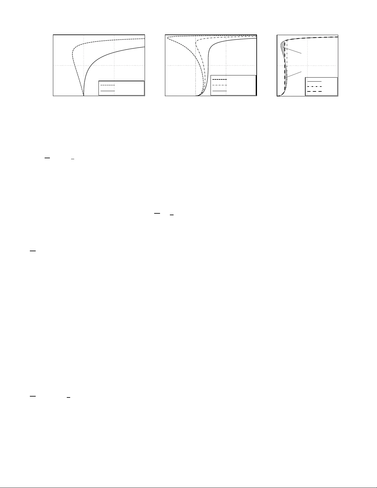
MANUSCRIPT 1 Design and Analysis of LDGM-Based Codes for MSE Quantizati on Qingchuan W ang, Student Member , IEEE, Chen He, Memb er , IEEE, Abstract —Appr oaching the 1.5329-dB shaping (granular) gain limit in mean-squared e rror (M SE) quantization of R n is im- portant in a number of problems, n otably dirty-paper codin g. For this purpose, we start with a binary low-density generator - matrix (LDGM) code, and construct the q uantization codeb ook by p eriodically repeating its set of binary codewords, or them mapped to m -ary ones with Gray mapping. Th e qu antization algorithm is based on belief pr opagation, and it uses a decimation procedure to do the guessing necessary for conv er gence. Using the results of a tru e typ ical decimator (TTD) as refer ence, it is shown that the asy mptotic perf ormance of the propose d quantizer can be characterized by certain monotonicity conditions on the code’s ﬁxed point properties, wh ich can be analyzed with density ev olution, and degree distribut ion opti mization can be carried out accordingly . When the numb er of iterations is ﬁnite, the resulting loss is made amenable to analysis through the introduction of a reco very algorithm from “bad” guesses, and the results of such analysis enable fu rther optimization of th e pace of decimation and the degr ee distribution. Simulation results show th at th e proposed LDGM-b ased qu antizer can achieve a shaping gain of 1.4906 dB, or 0.0423 dB from the limit, and signiﬁcantly outp erf orms trellis-coded qu antization ( TCQ) at a similar computational complexity . Index T erms —granular gain, shaping, L DGM, source coding, decimation, belief p ropaga tion, density evolution, perfo rmance- complexity tradeoff I . I N T RO D U C T I O N T HE mean-squ ared erro r (MSE) quan tization p roblem o f R n [2, Sec. II-C] can be f ormulated as follows: 1 let Λ be a discrete subset o f R n (the quantizatio n c odeboo k , or simply code ) 2 and Q Λ : R n → Λ be a quantizer th at maps each The authors are with Department of Electronic Engineering, Shanghai Jiao T ong Univ ersity , Shangha i, 200240, China. E-mail: { r6144, chenhe } @sjtu.edu.cn. This paper was supported in part by National Natural Science F oundati on of China Grant No. 6077210 0 an d in part by Scie nce & T echno logy Committee of Shanghai Municipality Grant No. 06DZ15013. Part of the material in this paper has been presented in [1] at IE EE Global Communicati ons Conferenc e, W a shington, DC, Novembe r 2007. 1 Notatio nal con v ention s: Z and R are respecti vel y t he set of inte gers and real numbers. k·k is the Euclidean norm. |A| is the cardinalit y of set A . . = denotes asymptotic equa lity , usually with respect to block length n → ∞ . log( · ) , entrop y and mutual informati on are computed in base-2 , while ln( · ) and exp ( · ) are base- e . Bold letters denote sequences or vectors whose elements are indicate d by subscripts, e.g. y = ( y 1 , . . . , y n ) , and sub-sequenc es are denote d by y j i = ( y i , y i +1 , . . . , y j ) or y S = ( y i ) i ∈S . Addition and mult iplica tion on sets apply eleme nt-by-el ement, e.g. U +2 Z n = { u + (2 d 1 , . . . , 2 d n ) | u ∈ U , d i ∈ Z } . x mo d [ a, b ) (or simply ( x ) [ a,b ) ) is deﬁne d as t he unique e lement of ( x − ( b − a ) Z ) ∩ [ a, b ) , and similarl y x mo d [ a, b ) n or ( x ) [ a,b ) n is the u nique ele ment of ( x − ( b − a ) Z n ) ∩ [ a, b ) n . The unit “b/s” means “bits per symbol”. 2 Ref. [2] assumes that Λ is a lattic e, but in practic e neither the trellis in TCQ nor the non-binar y codebook s proposed here are lattices. T herefore , we allo w Λ to be any discrete set, and deﬁnitions are modiﬁed accordingly . y ∈ R n to a nearby codew ord Q Λ ( y ) ∈ Λ . The mean-squar e quantization er ror, averaged over y , is gi ven by σ 2 = lim sup M →∞ 1 (2 M ) n · 1 n Z [ − M ,M ] n k y − Q Λ ( y ) k 2 d y . (1) The objective is to design Λ and a p ractical quan tizer Q Λ ( · ) such that the scale-n ormalized MSE G (Λ) = σ 2 ρ 2 /n is minimized, 3 where ρ is the codew ord density ρ = lim sup M →∞ 1 (2 M ) n | Λ ∩ [ − M , M ] n | . (2) In this pap er we consider asympto tically large dimension- ality n . By a v olume argum ent, it is easy to ﬁnd a lower bound G ∗ = 1 2 π e for G (Λ) . This bou nd can be approa ched by the nearest-n eighbo r q uantizer with a suitable r andom codebo ok e.g. in [2], whose codewords’ V oronoi region s are asymptotically spherical, but such a qu antizer has expone ntial complexity in n and is thus imp ractical. Th e simplest scalar quantizer Λ 1 = Z n , on the other hand, has the 1.532 9-dB larger G 1 = G (Λ 1 ) = 1 12 , wh ich co rrespon ds to the well- known 1. 53-dB lo ss of scalar quantization . In general, we call 10 log 10 ( G (Λ) /G ∗ ) the shaping loss of a qu antizer, and it is also the gap of th e g ranular gain a nd shaping gain d eﬁned in [3], for source and chan nel coding respectively , tow ard the 1.53-d B limit. MSE qu antizers with n ear-zero shaping losses are importa nt in both source and channel coding . In lossy sou rce coding , the shaping loss n aturally dictates rate-d istortion per forman ce at high rates [3 ]. I n channel coding on Gau ssian channels, MSE quan tizers can be u sed for shaping to make the chan nel input closer to th e optim al Gaussian d istribution [4]. Basi- cally , instead of tran smitting the ch annel-co ded and Q AM- modulated sign al u (each ele ment o f u correspo nding to on e symbol in the code bloc k), we transmit x = u − a with a = Q Λ ( u ) ∈ Λ , which sho uld be closer to Gaussian. u and a are separated at the rece i ver side, an d th e shap ing loss determines the achievable gap f rom chan nel capacity at high SNRs. Shaping is particular ly im portant in dirty-paper coding (DPC) [5] on the c hannel y = x + s + z , (3) where x is the tran smitted sign al, s is the interferen ce known only at the transmitter, an d z is the “MMSE-adjusted” n oise. Using an MSE quantize r , arbitra rily large s can be p re- cancelled withou t signiﬁcantly increasing sign al power by transmitting x = u − s − a , with a = Q Λ ( u − s ) , (4) 3 This agrees with the deﬁniti on of G (Λ) for latti ces in [2]. MANUSCRIPT 2 so that the received sig nal y = u − a + z . (5) Again, th e recei ver m ust separate u and a , and the shaping loss determines the ach iev able gap from c hannel capa city . In this case, howe ver , due to th e lack of rec eiv er-side knowledge of s , the r ate loss caused by non-id eal shaping is mo st sign iﬁcant at low SNRs an d can b e a sign iﬁcant fractio n of chann el capacity [6]–[9 ]. For exam ple, th e shaping qu antizer in [ 9] has 0. 15 dB shaping loss, correspon ding to a rate loss of 0.025 b/s, yet in the 0 .25-b /s DPC system this is alread y 1 0% of the rate and is responsible for 0.49 dB of its 0.83-dB gap from capacity . Apart from its obviou s application in steganography [10], DPC and its extension to vector channels (similar in prin ciple to vector precod ing [ 11] but done in b oth time an d spatial domains) are also essential in approachin g the capacity of vector Gau ssian broadc ast channels such as MIMO do wn link, therefo re the design of near - ideal MSE quan tizers is of gr eat interest in these applications. Currently , near-optimal MSE quantizer s usually employ trellis-coded quantization ( TCQ) [1 2], in wh ich Λ = U + 2 Z n or U + 4 Z n with U being respectively the codeword set of a binary co n volution co de or a 4-ary trellis code. T he nu mber of r equired trellis states in creases very r apidly as the sh aping gain appro aches the 1 .53-d B limit, an d the compu tational complexity and memory requir ement a re thus very high . This is p articularly b ad at the r eceiv er side of DPC systems, where the BCJR (Bahl-Cocke-Jeline k-Ravi v) algo rithm must be run many times on the trellis in an iterativ e fashion to separate u and a [9], resulting in a time complexity pr oportion al to both the number of trellis states and the outer iteration count. Inspired by the effectiveness of Turbo and low-density parity-ch eck (LDPC) cod es in chann el cod ing, it is natural to con sider the use o f sparse-grap h codes in quantiza tion. In [13] Turbo codes are used in quan tization of uniform source s, but con vergence issues make the scheme usable only for very small block sizes n , an d the shaping loss is thu s unsatisfactory . In [1 4]–[1 6], it is sh own that lo w-de nsity generato r matrix (LDGM) codes, being the duals of LDPC cod es, are good fo r lossy comp ression of binary sou rces, and practical qua ntiza- tion alg orithms based on belief propag ation (BP) and su rvey propag ation (SP) ha ve also bee n proposed in [17] and [1 8], but these works consider b inary so urces o nly . Pr actical algorith ms for the MSE q uantization of R n with LDGM codes h av e not received much attention befor e. Even in the binary case, little has been done in the analy sis of the BP quan tizer’ s beh avior and the optimiza tion of the LDGM code for it. In [1], we have addre ssed the pro blem of MSE q uantization using LDGM-based codes of structure Λ = U + m Z n , known as m -a ry codes , where each u ∈ U is a codew o rd of a binary LDGM co de wh en m = 2 , an d is the com bination of two codewords, each fro m a binary LDG M cod e, by Gray mapping when m = 4 . Th e degree distrib u tions of the co des are optimized u nder th e er asure appro ximation, and shap ing losses as low as 0.056 dB have been d emonstrated . In this p aper, we w ill impr ove u pon the results in [1] by using better analytical techniqu es and more accurate method s for co de op timization. W e start in Section II by analyzin g the m inimum shap ing loss achie vable by this m -ary structur e using random-c oding argum ents. Alth ough binary quantization codes hav e sign iﬁcant random-co ding loss, th ey ar e analyzed ﬁrst due to their simplicity . In Sec tion III , we present the quantization algorithm for bina ry cod es, which consists, like [18], of BP and a gue ssing ( “decimation” ) p rocedu re to aid conv e rgence. Like LDPC, degre e distribution plays an impor tant role in the perfor mance o f LDGM qua ntization co des, but the use of dec imation makes direct an alysis difﬁcult. T o solve this problem , we propo se th e typical de cimator (TD) as a subopti- mal b ut analytically more tractab le version of the decimation algorithm , an d analyze ﬁrst its use in the simp ler binar y erasure q uantization (BEQ) prob lem in Section IV, which also fo rms the basis for the erasure approximatio n in [1]. W e ﬁnd that the TD can ob tain asy mptotically correct extrinsic informa tion for decimation, and a s olution to BEQ can be found with such infor mation, as long as th e code ’ s extended BP (EBP) extrinsic informatio n tr ansfer (EXIT) cu rve [19] characterizin g the ﬁxed po ints o f th e BP pr ocess satisﬁes certain monotonicity co nditions . For a gi ven LDGM cod e, the most d ifﬁcult BEQ p roblem it can solve is th en p arametrized by a mono tonicity thr eshold I thr c , and th e degree distribution can b e op timized by maxim izing this I thr c . In Section V, these argumen ts are extended to our MSE quantization p roblem, and similar monoton icity cond itions are obtained, which can be checked by quantized d ensity e volution (DE). These DE results can be visualized with mo diﬁed EXIT curves, and a similar method to the BEQ case can then be used f or d egree distribution optim ization. W e have assumed itera tion cou nts L → ∞ in the above analysis. In Section VI, we proce ed to an alyze the impact of ﬁnite L . W e will show tha t a ﬁnite L causes “bad” guesses in decimation, a nd a r ecovery a lgorithm is sometimes requ ired for BP to co ntinue n ormally afterwards. Wi th r ecovery , the loss due to ﬁn ite L can b e characteriz ed b y the delta-area A i between the EBP cu rve and the actual trajectory , which will be used in the subsequen t op timization o f the pace of dec imation as w ell as the degree distribution. All these results are extended to m -ary codes ( where m = 2 K ) in a straightforward man ner in Section VI I. Nu merical results on MSE per forman ce in Section VIII shows that LDGM quan tization cod es optimized with the afo remention ed methods h av e the expected good perfo rmance and can ach ie ve shaping losses of 0.2 676 dB at 99 iterations, 0.07 41 dB at 1022 and 0.042 3 dB at 8356 iteration s, the latter two of which are far be tter than what TCQ can reason ably o ffer and ar e also signiﬁcantly better than th e re sults in [1 ]. I ndeed, a heuristical analysis on the asy mptotic loss-complexity tradeoff ca rried out in Sectio n I X indicates th at LDGM q uantization codes can achieve th e same sha ping loss with far lower complexity th an TCQ. W e conclud e the paper in Section X. I I . P E R F O R M A N C E B O U N D S O F m - A RY Q UA N T I Z E R S In this pap er , we consider Λ with a perio dic structure Λ = U + m Z n , where U is a set o f 2 nR codewords f rom { 0 , 1 , . . . , m − 1 } n with ea ch u = u ( b ) ∈ U labeled by a MANUSCRIPT 3 binary sequ ence b ∈ { 0 , 1 } nR . W e call Λ an m -a ry rate- R quantization co de . In this section, we will analyze the achiev ab le shaping loss by this periodic struc ture. Giv en the source sequen ce y ∈ R n , for e ach u = u ( b ) ∈ U the nearest seq uence to y in u + m Z n is x ( b ) = y − z ( b ) , where z ( b ) = ( y − u ( b )) I n is the quantization error and I = [ − m 2 , m 2 ) . The quan tizer has then to minimize k z ( b ) k over all b ’ s, or equiv alen tly , to maxim ize q y ( b ) = e − t k z ( b ) k 2 = n Y j =1 e − t ( y j − u j ( b )) 2 I (6) for some co nstant t > 0 . The chosen b is denoted b y , th e correspo nding quantizatio n erro r is z y = z ( b y ) , and the resulting MSE (1) then b ecomes 4 σ 2 = 1 m n · 1 n Z [0 ,m ) n k z y k 2 d y = 1 n Z [0 , 1) n D k z ˜ y + a k 2 E d ˜ y , (7) where h·i d enotes averaging over a ∈ { 0 , 1 , . . . , m − 1 } n . A. Lower Bound of Qu antization Err or Giv en Λ , for each source sequence y ∈ [0 , m ) n , let Q y = X b ∈{ 0 , 1 } nR q y ( b ) . (8) Since q y ( b y ) ≤ Q y , we can lower-bound the mean-squ are quantization error 1 n k z y k 2 as 1 n k z y k 2 = − 1 nt ln q y ( b y ) ≥ − 1 nt ln Q y . (9) Now let y = ˜ y + a with ˜ y ∈ [0 , 1) n and a ∈ { 0 , 1 , . . . , m − 1 } n , and average over a , then f rom Jensen’ s inequality 1 n D k z ˜ y + a k 2 E ≥ − 1 nt h ln Q ˜ y + a i ≥ − 1 nt ln h Q ˜ y + a i , (10) where h Q ˜ y + a i can easily be found to be h Q ˜ y + a i = 2 nR m n n Y j =1 Q ˜ y j , with Q ˜ y = m − 1 X a =0 e − t ( ˜ y + a ) 2 I . (11) σ 2 in (7) can b e lower -boun ded b y integrating (10) over ˜ y . For as ymptotically large n , we only need to con sider (strongly) typical ˜ y with respect to the unifor m distribution o n [0 , 1) , i.e. whose n elements are near ly unifo rmly d istributed over [0 , 1 ) . W e thus have σ 2 ≥ − 1 nt Z [0 , 1) n ln h Q ˜ y + a i d ˜ y (12) . = 1 t  ln m − R ln 2 − Z 1 0 ln Q ˜ y d ˜ y  . (13) 4 For large n , (7) is mostly just an a vera ge ov er strongly typical y with respect to the uniform distributio n on [ 0 , m ) , i.e. those whose elemen ts are approximat ely uniformly distribut ed over [0 , m ) , and the rest of this paper considers such y onl y . In shaping and DPC ap plicat ions, y can be a modul ated signal that does not follo w the uniform distrib ution, and in such cases it m ay be necessary to “dither” y before quantiz ation by adding to it a random sequence uniformly distrib uted in [0 , m ) n and known by the dequantiz er , in order to obtain the expe cted MSE performance. This bo und hold s f or any t > 0 and is found to be tigh test for t satisfying H t = lo g m − R (this t is hence denoted t 0 ( R ) ), when it beco mes σ 2 ≥ P t . H t and P t are d eﬁned as H t = − Z I p z ( z ) log p z ( z ) dz , (14) P t = Z I z 2 p z ( z ) dz , (15) p z ( z ) = e − tz 2 Q ˜ y , z ∈ I , ˜ y = z mo d [0 , 1) . (16) B. Ac h ievable Quantization E rr or with Ran dom Codin g For asy mptotically large n , we will see that th e aforemen - tioned lo w er bound is actually achievable by random co ding, that is, with the 2 nR codewords in U indepen dently and unifor mly sampled from { 0 , 1 , . . . , m − 1 } n (allowing fo r duplicates) an d u sing th e nearest-neighb or q uantizer . Again we assum e y ∈ [0 , m ) n , and sinc e the MSE 1 n k z y k 2 is boun ded for any y , we c an consider only ty pical y ’ s with respect to the uniform distrib ution on [0 , m ) . Deﬁne U y = n u ∈ { 0 , . . . , m − 1 } n    k ( y − u ) I n k 2 ≤ n P t o (17) as the set of possible co dew o rds that ar e “su fﬁciently close” to y , and we can compute 1 n log |U y | with large de viatio n theory . I f it is larger than log m − R , with asympto tically h igh probab ility U ∩ U y 6 = ∅ , th us som e x ∈ U + m Z n can b e fo und whose MSE toward y is no more than P t . Sin ce this is true for most typica l y , the average MSE σ 2 cannot exceed P t by more tha n a vanishingly small value. T o comp ute 1 n log |U y | for a typ ical y , we deﬁne the type p y ( u ) o f a sequenc e u as th e fraction of each u ∈ { 0 , 1 , . . . , m − 1 } at the position s in u whose co rrespond ing elements in y are app roximately y . Denoting the num ber o f sequences u with this type as N [ p y ( u )] , we have 1 n log N [ p y ( u )] . = 1 m Z m 0 H y ( u ) dy , (18) where H y ( u ) is the entropy H y ( u ) = − m − 1 X u =0 p y ( u ) log p y ( u ) , (19) and u ∈ U y becomes the con straint 1 m Z m 0 m − 1 X u =0 ( y − u ) 2 I p y ( u ) ! dy ≤ P t . (20) According to large deviation theory , 1 n log |U y | is asymp toti- cally th e maximum of (18) u nder the con straints (20) and p y ( u ) ≥ 0 , m − 1 X u =0 p y ( u ) = 1 , y ∈ [0 , m ) . (21) This is a co n vex functional optimization problem over p y ( u ) (a function of both y and u ), which can b e easily solved with Lagrang e multipliers. T he m aximizing p y ( u ) is foun d to be p y ( u ) = e − t ( y − u ) 2 I Q ˜ y , ˜ y = y mo d [0 , 1) , (22) MANUSCRIPT 4 and the resulting 1 n log |U y | . = H t . (23) By the argument above, as long as H t > log m − R , i.e. t < t 0 ( R ) , rand om cod ing can achieve σ 2 ≤ P t for asym ptotically large n . C. Mar ginal Distribution of Quan tization Err or From the p y ( u ) r esult in (22), th e marginal distribution of an individual z j = ( y j − u j ) I under random cod ing can also be o btained as p z ( z ) = 1 m Z m 0 m − 1 X u =0 p y ( u ) δ ( z − ( y − u ) I ) ! dy (24) = 1 m Z m 0 m − 1 X u =0 e − tz 2 Q ˜ y δ ( z − ( y − u ) I ) ! dy (25) = e − tz 2 Q ˜ y , z ∈ I , (26) where δ ( · ) is the Dir ac delta fun ction and ˜ y = z mo d [0 , 1 ) = y mod [0 , 1) . Th is is simp ly the p z ( z ) in (1 6), and H t in (14) and P t in (1 5) are r espectively the entropy and average power of th is d istribution. D. Th e Random-Cod ing Lo ss W e have shown tha t a ran dom quantization codeb ook with the n earest-neigh bor quan tizer is asymp totically optim al among rate- R quan tization codes of the for m Λ = U + m Z n . Therefo re, its shaping loss re presents the per forman ce limit of su ch co des, and can b e viewed as the cost incurred b y the period- m structure. For asymptotically large n , the random m -ary q uantizer has average MSE σ 2 = P t with t = t 0 ( R ) and density ρ = 2 nR /m n , so th e achieved G (Λ) = σ 2 ρ 2 /n = P t (2 R /m ) 2 . The shaping lo ss 10 lo g 10 ( G (Λ) /G ∗ ) can then be expressed as 10 log 10 ( P t /P ∗ t ) , where P ∗ t = 1 2 π e ( m/ 2 R ) 2 is the power of a Gaussian with en tropy H t = lo g m − R . W e called it the random-cod ing loss , and it is plo tted in Fig. 1 fo r m = 2 and m = 4 . For large m and moderate R , Q ˜ y in (11) approach es a co nstant, p z ( z ) is close to a Gaussian distrib ution, thu s P t ≈ P ∗ t and the ra ndom-c oding lo ss is close to ze ro. I I I . T H E B I N A RY L D G M Q U A N T I Z E R As random quantization codes with the nearest-neig hbor quantizer are obviously im practical to im plement, it is natura l to look into sparse-graph co des a s practical cand idates for achieving n ear-zero shap ing losses. In [ 14], it has bee n shown that LDPC codes ar e u nsuitable for BEQ but LDGM codes work well, therefo re we will also u se LDGM codes in MSE quantization . W e con sider the simplest m = 2 case ﬁrst, and in Section VI I we will look into code s with larger m that ar e not as limited by the rand om-cod ing loss. W e thus consid er Λ = U + 2 Z n with U bein g the codew o rd set of a n LDGM code, i.e. each u ∈ U is o f the form u = c = bG , wher e b ∈ { 0 , 1 } n b , n b = nR an d the low-density generato r matr ix G = ( g ij ) n b × n is rando mly gen erated from 0 0 . 5 1 1 . 5 Random coding l oss (dB) 0 0 . 5 1 R (b/s) (a) binary code ( m = 2 ) 0 0 . 5 1 1 . 5 Random coding l oss (dB) 0 1 2 R (b/s) (b) 4-ary code ( m = 4 ) Fig. 1. Ra ndom-coding losses of binary and 4-ary quant ization code s. For binary quant izati on codes, the m inimum loss is approximatel y 0.0945 dB at t = 3 . 7 and R = 0 . 4130 b / s . For 4-ary codes, the minimum loss is only 0.0010 dB at approximately t = 2 and R = 0 . 9531 b / s . some d egree distribution that will be optimized below . Given such a code, q y ( b ) in (6) can be r epresented by the factor graph [20 ] in Fig. 2(a). 5 The c -no des ( shorthand f or the factor nodes c j , j = 1 , . . . , n ) represen t the relationsh ip c = bG , whereas each factor e − t ( y j − c j ) 2 I in (6 ) is included in the prior λ c j on v ar iable c j as λ c j ( c ) = 1 Q ˜ y j e − t ( y j − c ) 2 I = p z (( y j − c ) I ) , (27) where Q ˜ y j (with ˜ y j = y j mo d [0 , 1) ) serves as the n ormaliza- tion factor . The belief pr o pagation alg orithm (also known a s the sum- produ ct algo rithm) can then be run on this factor grap h. Unlike the case of LDPC de coding, here BP does not usually con verge by itself. 6 Instead, we rely on BP to g enerate “extrinsic probab ilities” ν b i for each b i after a numb er o f iteratio ns, with which hard decisions are made on some b i ’ s (called decimation following [17]) . Subseq uent BP iterations use these hard decisions as priors λ b i , and th e resultin g u pdated ν b i ’ s are used for mo re decimation s. This iterative pr ocess contin ues until a d eﬁnite b is obtained th at h opefu lly has a large q y ( b ) and thus a small quantization error . Th is q uantization algorithm is shown in Fig. 3 , with a BP part and a decimation p art in each iteration. As is in tuitiv ely reasonable, each time we decimate 5 In the factor graph, symbols such as b i and c j denote va riable and facto r nodes, while b i and c j are the varia bles themselves. N bc · j = N cb j · denote the set of indices i for whic h there is an edge conne cting b i and c j . In belief propagat ion, λ b i is the priors on va riable b i , ν b i is the computed extrinsi c probabil ities for b i , µ bc ij denotes a message from node b i to c j , and so on. The priors, posteriors and m essages are all probabilit y distrib utions [20], in this case over { 0 , 1 } , and here we represent them by probability tuples (rather than L -value s, which are equi val ent). Fo r e xample, λ b i is viewed as a tuple ( λ b i (0) , λ b i (1)) satisfying λ b i (0) + λ b i (1) = 1 (the normalizati on is done implici tly), which correspo nds to L -v alue ln( λ b i (0) /λ b i (1)) . “ ⊙ ” and “ ⊕ ” refer to the var iable- node and check-node operation s in LDPC literat ure, i.e. ( µ 0 , µ 1 ) ⊙ ( µ ′ 0 , µ ′ 1 ) = ( µ 0 µ ′ 0 , µ 1 µ ′ 1 ) (implici tly normalized) and ( µ 0 , µ 1 ) ⊕ ( µ ′ 0 , µ ′ 1 ) = ( µ 0 µ ′ 0 + µ 1 µ ′ 1 , µ 0 µ ′ 1 + µ 1 µ ′ 0 ) . 0 = (1 , 0) , 1 = (0 , 1) and ∗ = ( 1 2 , 1 2 ) are respecti vely the “sure-0”, “sure-1” and “unknown” messages. H ( µ ) = − µ 0 log µ 0 − µ 1 log µ 1 is the entropy function for µ = ( µ 0 , µ 1 ) . 6 Intuiti vel y speakin g, when doing L DPC decoding with SNR higher than threshold , the transmitt ed code word is usual ly much close r to the receiv ed sequence (and thus much more likely ) than any other codew ord, allo wing BP to con verge it. In the case of quantiza tion with LDGM codes, there are usually a large number of similarly close code words to the source sequence, and BP cannot by itself make a decision among them. MANUSCRIPT 5 b 1 b 1 b n b b n b c 1 c 2 c n c 1 c 2 c n (a) original form b 1 b 1 b n b b n b c 1 c 2 c n ˜ c 1 ˜ c 2 ˜ c n a 1 a 1 a 2 a 2 a n a n (b) perturbed form Fig. 2. The factor graph of the binary LDGM quantize r . Circles are vari able nodes and black squares are factor nodes. The gray area contains random b -to- c edges, and each edge from b i to c j correspond s to g ij = 1 in the generat or matrix G . W e mostly use the original form (a) with the priors λ c j ( c ) = p z (( y j − c ) I ) . T he equiv alent “perturbed” form (b) is used in Section V -A, where ˜ y = y mo d [0 , 1) n , a = ( y − ˜ y ) mo d 2 ∈ { 0 , 1 } n , and ˜ u = ˜ c = ( c − a ) mo d 2 . Wit h y ﬁxed, each prior λ a j is a hard decision a j . Sinc e z = ( y − c ) I = ( ˜ y − ˜ c ) I , the p rior on ˜ c j is λ ˜ c j (˜ c ) = p z (( ˜ y j − ˜ c ) I ) . the “most certain ” bit b i ∗ , with i ∗ = a rg max i ∈E max b ∈{ 0 , 1 } ν b i ( b ) , (28) and it is decimated to its most likely value b ∗ = a rg max b ∈{ 0 , 1 } ν b i ∗ ( b ) . (29) This is called the gr ee dy decima tor (GD) . Alternatively , f or the conv enience of an alysis we will also look at th e typ ical decimator , implemen table but with worse p erform ance in practice, in which the bit index i ∗ to d ecimate is chosen random ly in E (the set of y et un decimated bits) with equ al probab ilities, and its d ecimated value b ∗ is b ∈ { 0 , 1 } with probab ility ν b i ∗ ( b ) . The nu mber of bits to d ecimate is co ntrolled thro ugh the estimated m utual inform ation I b c in b -to- c messages (i.e. the µ b c ij ’ s), which is made to incr ease by about ∆ I min b c in each iteration. This amount of inc rease ∆ I min b c , possibly a function of the cu rrent I b c and hence called th e pace of decimation , makes th e algorithm termin ate within L 0 iterations if fo llowed exactly , tho ugh th e actual iteration co unt L can be somewhat d ifferent. U niform pacin g is used in [ 1], i.e. ∆ I min b c is a con stant 1 /L 0 . I n this pap er , th e pacing is op timized in Section VI-D to obtain somewhat better MSE perform ance. Increasing L 0 also improves MSE perfo rmance, but more iterations w ould be necessary . The decim ation algo rithm can either b e un thr ottled or thr ot- tled . The unthrottled version used in most of our simulations simply decimates un til the increase of I b c in the iteration reaches ∆ I min b c . In the throttled version introd uced in [1], the amount of d ecimation p er iter ation is instead con trolled by δ max , which is smoothly ad apted, as shown in Fig. 3, to m ake I b c increase e ventually at the desired pace. More will be said on the decimation algorithm in Sec- tion VI, but we will ﬁrst discuss the op timization of LDGM ’ s λ c j ( c ) ⇐ p z (( y j − c ) I ) , j = 1 , . . . , n , c = 0 , 1 {I = [ − 1 , 1) } µ bc ij ⇐ ∗ , i = 1 , . . . , n b , j = 1 , . . . , n λ b i ⇐ ∗ , i = 1 , . . . , n b E ⇐ { 1 , 2 , . . . , n b } { the set of bits not yet decimat ed } δ max ⇐ 0 , I bc ⇐ 0 repe at { belie f propagatio n ite ration } f or j = 1 to n do { BP computati on at c j } µ cb j i ⇐ λ c j ⊕  ⊕ i ′ ∈N bc · j \{ i } µ bc i ′ j  , i ∈ N cb j · end for f or i = 1 to n b do { BP computation at b i } µ bc ij ⇐ λ b i ⊙  ⊙ j ′ ∈N cb · i \{ j } µ cb j ′ i  , j ∈ N bc i · ν b i ⇐ ⊙ j ′ ∈N cb · i µ cb j ′ i end for I + bc ⇐ 1 − ( n b d b ) − 1 P i,j H ( µ bc ij ) { estimate ne w I bc } δ ⇐ 0 { amount of decimat ion so far in this iteratio n } Set ∆ I min bc accordi ng to the desired pace (e.g. to (101)) if I + bc < I bc + ∆ I min bc then { little progress, do decimation } repe at i ∗ ⇐ arg max i ∈E max b ν b i ( b ) { b i ∗ is the most certain bit. . . } b ∗ ⇐ arg max b ∈{ 0 , 1 } ν b i ∗ ( b ) { . . . whose likel y v alue is b ∗ } δ ⇐ δ + ( − l og ν b i ∗ ( b ∗ )) I + bc ⇐ I + bc + ( n b d b ) − 1 P j ∈N bc i ∗ · H ( µ bc i ∗ j ) λ b i ∗ ⇐ b ∗ , µ bc i ∗ j ⇐ b ∗ , j ∈ N bc i ∗ · { decimat e b i to b ∗ } E ⇐ E \{ i ∗ } until δ > δ max or I + bc ≥ I bc + ∆ I min bc or E = ∅ end if δ max ⇐ max(0 . 8 δ max , 1 . 25 δ ) I bc ⇐ I + bc until E = ∅ b i ⇐ 0 (resp. 1 ) if λ b i = 0 (or 1 ), i = 1 , . . . , n b c ⇐ bG , u ⇐ c z j = ( y j − c j ) I , x j = y j − z j , j = 1 , . . . , n Fig. 3. The binary quantiz ation algo rithm. T he throt tled version is sho wn abov e, while the unthrottled versi on is without the δ > δ max conditi on in the until statement. The choice of i ∗ and b ∗ correspond s to the greedy decimator . degree distribution and the choice of t in Section s IV and V. I V . D E G R E E D I S T R I B U T I O N O P T I M I Z AT I O N F O R B I NA RY E R A S U R E Q U A N T I Z A T I O N Like LDPC codes, LDGM q uantization codes requ ire op - timized degree distributions fo r g ood MSE p erforma nce. The perfor mance o f LDGM quan tizers has b een analyzed previ- ously in [ 15] f or binary sou rces, but this analysis, based on codeword-counting arguments, is applicable on ly to near est- neighbo r quantizatio n and n ot very usefu l fo r the above BP quantizer . I n [1 7]’ s tre atment of LDGM quantizatio n of b inary sources, degree distributions of good LDPC co des in [21 ] are used directly , inspired by the dua lity between source and chan - nel codin g in the er asure case [1 4]. In ou r previous work [1 ], LDGM degree d istributions are in stead designed by directly ﬁtting the EX IT curves under the erasur e ap pr oximation (EA), also known as the BEC ( binary erasure chan nel) app roximatio n [22]. Both methods perform well, but they ar e heuristic in their analysis o f decimation, and may th us be subop timal. In this and th e next section, we will give a detailed anal- ysis o n degree distribution op timization of BP-b ased LDGM quantizers that p roperly takes decimatio n into accou nt, which should a llow better MSE p erforman ce to be attain ed. Under the erasure app roximation , we are in effect designing a n LDGM quantization code for the simpler binary erasur e q uantization MANUSCRIPT 6 problem and using it in MSE quantization . 7 Therefo re, we will ﬁrst fo cus on BEQ in th is section, and in Section V the methods given her e will b e extend ed to MSE quan tization, with or witho ut the erasure approximatio n. A. Binary Erasur e Quantization The binary erasure quan tization pro blem can be formula ted as follows [14]. The sou rce sequence has the form y ∈ { 0 , 1 , ∗} n , where “ ∗ ” de notes erased p ositions and o ccurs with probab ility ǫ . A binary cod e U co nsisting of 2 nR codewords u = u ( b ) ∈ { 0 , 1 } n , ea ch labeled b y b ∈ { 0 , 1 } nR , is then designed according to ǫ an d th e rate R . For each y , the quantizer sho uld ﬁnd a c odeword u ∈ U such that y j = u j or y j = ∗ for all j = 1 , . . . , n , i.e. u agre es with y on all non-er ased positions. The number of non -erased positions in a gi ven y is d enoted b y n ne , which is ap proxima tely n (1 − ǫ ) for large n . Ideally n b = n R can be a s small as this n (1 − ǫ ) , i.e. R = 1 − ǫ , but in p ractice high er rate s are necessary . Similar to (6), q y ( b ) can be deﬁned as q y ( b ) = n Y j =1 q y j ( u j ( b )) , q y j ( u j ) = ( 1 y j = u j or ∗ , 0 otherwise , (30) and the qua ntizer can equiv alen tly ﬁn d, f or a given y , some b such th at q y ( b ) > 0 (which then equals 1). When U is the c odeword set o f an LDGM code and u = c = bG as in Sectio n II I, q y ( b ) ca n be descr ibed by the factor graph in Fig. 2( a) as well, where each λ c j ( c ) is a n ormalized version of q y j ( c ) , i.e. λ c j is 0 , 1 or ∗ if y j is resp ectiv ely 0 , 1 , ∗ . Ap art from this d ifference in λ c j , the algorithm in Fig. 3 with the typical de cimator can be used h ere f or th e purp ose of analysis, thoug h the recovery alg orithm in Section VI-B will be n ecessary f or g ood p erform ance in pr actice. The BEQ problem may alter natively be vie wed as a set o f linear equations bG ne = y ne (31) over the binary ﬁeld GF (2) = { 0 , 1 } , whe re G ne and y ne are the n ne columns of G and y that corre spond to non-er ased positions of y . Denoting by n r the rank of G ne , (3 1) then has 2 n b − n r solutions f or 2 n r of the 2 n ne possible y ne ’ s, and for other y ne ’ s the re is no solution at all. W e ﬁrst assume th at (31) has a set B of 2 n b − n r solutions, then p y ( b ) = 2 − ( n b − n r ) q y ( b ) is a probability distribution for b that is uniform over B . Using this p y ( b ) , similar to th e BP- derived extrinsics ν b i , the true extrinsic pro babilities ν b ∗ i of b i can n ow be deﬁned as ν b ∗ i ( b ) = p y ( b i = b | b F \{ i } = b ∗ F \{ i } ) , i = 1 , . . . , n b , (32) which depen ds on th e set F o f decimated bits and their decimated values b ∗ F . No te that ν b ∗ i can only be 0 , 1 , o r ∗ : it is b if all solutions with b F \{ i } = b ∗ F \{ i } have b i = b ∈ { 0 , 1 } , 7 In this paper we only consider codes chosen randomly , through random edge assignment, from the LDGM code e nsemble with a giv en degree distrib ution, therefore only the degree distribut ion is subject ed to optimiza tion, and we will not distingui sh between codes and degre e distribu tions. and oth erwise th ere m ust b e the same numb er o f so lutions with b i = 0 and with b i = 1 , mak ing ν b ∗ i = ∗ . W ithou t loss of genera lity , the typical decimator can b e assumed to d ecimate in the ord er of b 1 , b 2 , . . . , b n b . Decom - posing p y ( b ) into p y ( b ) = p y ( b 1 ) p y ( b 2 | b 1 ) · · · p y ( b n b | b n b − 1 1 ) , (33 ) each factor p y ( b i | b i − 1 1 ) is then the ν b ∗ i after th e decimatio n of b i − 1 1 into b i − 1 , ∗ 1 . W e therefor e con struct the ﬁctitio us true typical decimato r (TTD), which is just like th e TD except that decimatio n of b i is don e according to ν b ∗ i rather than ν b i . Moreover , the TTD shares the sour ce of randomn ess with the TD, so decim ation is still d one in the o rder o f b 1 , . . . , b n b , an d each b i is decimated to the same value except to account for the dif f erence b etween ν b i and ν b ∗ i . 8 The TTD i n effect samples a b ∗ accordin g to the probab ility distribution p y ( b ) , so it mu st yield a ra ndom solution b ∗ ∈ B . If , for every i = 1 , . . . , n b , the TD at the time of b i ’ s decimatio n has ν b i = ν b ∗ i , then it will run syn chrono usly with the TTD and yield the same solutio n in B . Oth erwise, e.g. if ν b i = ∗ and ν b ∗ i = 0 for some i , then the TD might decimate b i to 1, which will eventually resu lt in a contradiction . Therefo re, our ﬁrst requ irement for TD to ﬁnd a solution to ( 31) is th at BP must co mpute the co rrect extrinsic probabilities after enough iterations, which is hen ce called th e e xtrinsic pr oba bility cond ition . How , then, to ensure the existence of solution s to (31) fo r any y ne ? W e may deﬁne Q y with (8) which, fo r each y ne , giv es th e num ber o f so lutions to (3 1) and is 2 n b − n r for 2 n r y ne ’ s an d zero f or the rest. Q y , if no rmalized by 2 − n b , is again a un iform d istribution over these 2 n r y ne ’ s. W e then require n r = n ne , mak ing Q y a uniform distribution over all 2 n ne possible y ne ’ s, so that the BEQ p roblem h av e 2 n b − n ne solutions for any y ne . This is the other con dition fo r BEQ to be always solvable b y th e TD, h ence called the equi-pa rtition condition . For n → ∞ , th e two condition s ab ove are now suitable for analysis w ith density ev olution meth ods, which in th e BEQ case can be accurately done with EXIT charts, as will be discussed in the following subsections. B. F ixed P oints and EX IT Curves W e use b -regular, c -irregular LDGM codes fo r quantiza tion as suggested by the LDGM- LDPC d uality in [14]. Let d b be the r ight-degree o f all b -nodes, a nd den ote w c d as th e fr action of c -n odes with left-degree d and v c d = dw c d / ( Rd b ) as the correspo nding fraction o f ed ges. Assuming that the BEQ pro blem d oes have solutio ns fo r the gi ven y , with the one fo und b y TTD den oted b ∗ and u ∗ = c ∗ = b ∗ G . Assuming additio nally that our qua ntizer based on TD has dec imated a fraction I b of the b -n odes and has so far maintained synch ronization with th e TTD in decimation decisions, b ∗ is then co nsistent with the curre nt 8 For exampl e, the TD and the TT D can use the same i.i.d. random sequenc e τ 1 , τ 2 , . . . , τ n b in decimation with each τ i uniformly distribute d in [0 , 1) , and each b i is decimate d to 0 in the TD if τ i < ν b i (0) and in the TT D if τ i < ν b ∗ i (0) , and to 1 otherwise. In this way , the decimation results are alw ays the same if ν b i = ν b ∗ i , and are rarely differen t if ν b i and ν b ∗ i are close. MANUSCRIPT 7 0 0 . 5 1 I b , ext (bit) − 0 . 5 0 0 . 5 1 I b (bit) I c = 0 . 5000 I c = 0 . 3333 (a) EBP curves of (4 , 2) regul ar LDGM code 0 0 . 5 1 I b , ext (bit) − 0 . 5 0 0 . 5 1 I b (bit) I c = 0 . 6000 I c = 0 . 5176 I c = 0 . 4375 (b) EBP curve s of (5 , 3) regular LDGM code 0 0 . 5 1 I b , ext (bit) 0 0 . 5 1 I b (bit) A 1 A 2 EBP BP MAP (c) Comparison of EBP , BP and MAP Fig. 4. The EBP curves of some ( d b , d c ) regular LDGM codes, in which all b -nodes hav e right-de gree d b and all c -nodes hav e left-degr ee d c . (a) The (4 , 2) regul ar code has rate R = 0 . 5 and monotonici ty threshold I thr c = 1 / 3 . For I thr c < I c ≤ R , part of the EBP curve lies in the I b < 0 half-pla ne, although I b is monotonica lly increa s ing once it becomes positi ve. This implies a violat ion of the equi-parti tion condition . For I c < I thr c , the monotonicity conditi ons are satisﬁed. (b) The (5 , 3) regular code has rate R = 0 . 6 and monotonici ty threshold I thr c = 7 / 16 = 0 . 4375 . When I c is reduced to 0.5176, the E BP curve no longer exten ds into the I b < 0 half-plane, but it is s till not monotonic until I c is further reduced to I thr c . (c) A comparison of the EBP , BP and MAP curves of the (5 , 3) regular code at I c = 0 . 5 , assuming that the results in [19] remain true. The area A 1 to the right of the MAP curve represents the b i ’ s whose ν b ∗ i = b ∗ i but ν b i = ∗ and thus violate the extri nsic probabil ity condi tion. That is, the va lues of these bits are determine d by pre vious decimati on results but not av ailable from BP at the time; they are apparen tly “guesses” until the y are “conﬁrmed” by an equa l number of equations encoun tered late r represented by A 2 . Here A 2 = A 1 , which intui tiv ely means that all conﬁrmations constrain earli er guesses rather than y ne , so the equi-pa rtition condition is satisﬁed. This is not the case for e.g. the (4 , 2) regular code at I c = 0 . 5 in (a): there the MAP and the BP curves overl ap with the EBP curv e in the I b ≥ 0 half-pla ne but does not e xtend to the left , and the area betwee n the E BP curv e and the I b = 0 axis represent “conﬁrmations” that, ha ving no earli er guesses, must be satisﬁed by y ne , therefore the equi-part ition condition is not satisﬁed. priors a nd can serve as the r eference cod ewor d : all µ b c ij and µ cb j i ’ s, with b i decimated or not, mu st be either b ∗ i or ∗ and never co ntradict the ref erence co dew o rd. Deno ting by e.g. I b c the av erage mutual informatio n (MI) in the µ b c ij ’ s from the previous iteration abou t their r espectiv e r eference values b ∗ i , which in this case is simply the fractio n of µ b c ij that e quals b ∗ i , 9 and using the usual fact that the factor graph becom es locally tree-like with hig h pr obability as n → ∞ , we can ﬁnd the E XIT c urve relatin g th e inp ut I b c for the c -node s and their output I cb , hence called the c -curve, to be I cb = I c X d v c d I d − 1 b c , (34) where I c is th e MI of the λ c j ’ s, in this case 1 − ǫ . Th e b -cu rve relating I cb and the outpu t I b c from the b -no des (d enoted by I + b c as it refers to the next iter ation) is likewis e I + b c = 1 − (1 − I b )(1 − I cb ) d b − 1 . (3 5) T o analyze the e xtrinsic probability condition, i t is necessary to look in to the behavior of BP’ s ﬁxed poin ts, which are characterized by the E BP EXIT curve ﬁrst prop osed in [1 9] for LDPC decod ing over BEC. Th e EBP curve relate s the a priori MI I b at ﬁxed points (i.e. the I b making I + b c = I b c ), I b = 1 − (1 − I b c ) / (1 − I cb ) d b − 1 , (36) and the extrin sic M I in th e ν b i ’ s, i.e. the fraction of ν b i that are b ∗ i rather than ∗ , I b , ext = 1 − (1 − I cb ) d b , (37) as I b c goes fr om 0 to 1 an d I cb giv en by (3 4). Fig. 4 shows the EBP cu rves of some codes fo r example. No te th at I b , ext 9 In this paper , all such MIs and EXIT curves are also a vera ged over the LDGM code ensemble with the give n degree distrib ution. Assuming that rele vant concentra tion results hold, for n → ∞ we can also talk about the con ver gence beha vior of a speciﬁc code using these ensemble-a veraged MIs. is a lw ays non -negativ e and m onoton ically increasing with I b c , but I b in (36) is not n ecessarily so. Every crossing the EBP curve makes with a constant- I b vertical line corr esponds to a ﬁxed p oint of BP at th is I b , and when the num ber of iteratio ns L → ∞ , it is clear that BP will follow th e m inimum- I b , ext ﬁxed point as I b goes from 0 to 1, f orming the BP EXIT curve in [19 ]. T he MAP (maxim um a po steriori probab ility) EXIT curve in [1 9, Deﬁnition 2] is simply th e relation ship between the fraction I b of d ecimated bits and the average true extrinsic MI in the ν b ∗ i ’ s, as is evident from [19, Theo rem 2 ], where the rand om vector b (curren tly taking value b ∗ ) is the X in [ 19], the b -priors λ b i are the BEC outpu t Y , an d the c - priors λ c j (or y ) are the additio nal observation Ω . Interestingly , our BEQ p roblem is now very similar to the LDPC d ecoding pro blem o n BEC con sidered in [19 ], as both inv olve a system of lin ear equ ations over GF(2) that has at least on e solution ( b ∗ for L DGM-based BEQ and the transmitted codeword for LDPC-over-BEC) con sistent with all pre vious guesses. 10 In particular, th e area a bove the MAP curve is H ( b | y ) /n b [19, Theo rem 1], with H ( b | y ) being the entropy of the afo remention ed p y ( b ) ; unde r the equ i-partition condition (31) sho uld hav e 2 n b − n ne . = 2 n b (1 − I c /R ) solutions, so this area is 1 − I c /R , an d the area below the MAP cur ve is I c /R , wh ile if th e equi-par tition co ndition is violated (31) will have more solutions for the cu rrent y (a nd no ne f or many other y ’ s), and the MAP curve will have a smaller ar ea below it. On the other han d, the area below the EBP curve c an be computed directly fr om (36) and (37); this area is also I c /R if v c 1 = 0 , an d when v c 1 > 0 it is deﬁn ed as the total gray area in Fig. 5, which is smaller tha n but close to I c /R . 10 The only dif ference is that the number of equation s in BEQ, n ne , is random where as in LDPC decoding ov er BEC it is al ways the number of check nodes. This should not be essential though. MANUSCRIPT 8 − 0 . 5 0 0 . 5 1 I b (bit) 0 0 . 5 1 I b , ext (bit) Z 1 0 (1 − I b ) dI b , ext dI bc dI bc = I c R − d b I c v c 1 I b , ext | I bc =0 = 1 − (1 − I c v c 1 ) d b Fig. 5. The area under the EBP curv e (the thick solid curve) when v c 1 > 0 . In such cases the E BP curve does not start from (0 , 0) , and we deﬁne the area below it as the total area of the two gray reg ions, whose respecti ve areas are shown in the ﬁgure. Note that the lower area 1 − (1 − I c v c 1 ) d b is sm aller than d b I c v c 1 , so the total area is smaller than I c /R , but is ve ry close to it in the codes we will encounter since d b I c v c 1 is at most 0.03 or so. If th e results in [ 19] on the r elationship between MAP , BP and EBP curves remain true, these thre e cur ves should be g i ven by Fig. 4(c). He uristic argum ents below the ﬁgu re sug gest th at the extrinsic pr obability and eq ui-partition cond itions above for the TD to solve th e BEQ problem ar e satisﬁed, with a vanishing fra ction o f exceptions as n → ∞ , if an d only if the EBP cu rve satisﬁes the f ollowing monoton icity conditions : 11 I b | x =0 ≥ 0 , (38) dI b dx ≥ 0 , x ∈ [0 , 1 ] , (39) where I b is viewed as a fun ction (36) of x = I b c . W e now prove this using similar methods to [19] . Necessity . Th e extrinsic probability cond ition mean s that ν b i = ν b ∗ i for all but a vanishing fr action of i ∈ { 1 , . . . , n b } at any I b after eno ugh iterations, which implies that the two h av e at least the sam e a verag e MI , i.e. the BP cur ve co incides with the MAP cur ve, th e area below which is in tu rn I c /R under the equ i-partition conditio n. Since the BP curve follows the minimum ﬁxed points on the EBP curve, and th e area un der the latter is at most I c /R , the two cur ves must coincid e a s well, which imm ediately leads to ( 38) and (3 9). Sufﬁciency . Und er (3 8) and (39), the BP curve obviou sly coincides with the EBP curve, and since ( 38) implies v c 1 = 0 , the area below them is I c /R . BP can never g i ve any infor- mation no t implied b y y and p revious decimation results, i.e. for any i we have either ν b i = ν b ∗ i or ν b i = ∗ , so the MAP curve can not lie below the BP curve and the area below it is at least I c /R . W e h av e also shown that the area below the MAP curve is at most I c /R , theref ore equ ality mu st h old and the e qui-partitio n co ndition is satisﬁed. Now that the MAP and BP curves also coincide, f or any I b the ν b i ’ s will have the nearly the same av e rage MI as the ν b ∗ i ’ s (with the difference vanishing after many iteration s when n → ∞ ) , and since any ν b i 6 = ν b ∗ i implies ν b i = ∗ and ν b ∗ i = b ∗ i and thus a difference in MI, it can o nly occur f or a vanishing ly small fr action o f i ’ s. Th erefore the extrinsic p robability conditio n also hold s.  11 Note that this has nothing to do with monotonicity with respect to a class of channe ls, which appears often in LDPC literat ure [23]. W e will see b elow that the monotonicity c ondition s are more easily satisﬁed for smaller I c , so for a giv en code, we can deﬁne the m aximum I c that satisﬁes them as the m onoton icity thr esho ld , denoted by I thr c . This is th e maximum (1 − ǫ ) for which the BEQ problem can, in an asymptotic sense, be solved by the TD. The same perfo rmance is expec ted for the greedy decimator, since in BEQ it is basically identical to TD. It should be noted that the monotonicity conditions are sufﬁ- cient f or the extrinsic prob ability and equi-pa rtition con ditions only in the sense that the fraction of violations ap proaches zero as the blo ck size n and the iteration count L go to inﬁnity . Ther efore, in practice some contradictio ns will occur in the T D, and some equa tions in ( 31) will be unsatisﬁed. In Section VI-B, we will prop ose a meth od to dea l with such contradictio ns, such th at th e n umber o f un satisﬁed eq uations remains a vanishing fraction of n . C. Optimizatio n o f th e Mon otonicity Threshold W e can now op timize th e degree distribution so that I thr c is maximized and app roaches its ideal value R . From (36) and (3 4), it is easy to show that the co ndition (38) is equiv alent to v c 1 = 0 , i.e. there are n o degree- 1 c - nodes. As fo r the second conditio n (39), d ifferentiating (36) with resp ect to x = I b c giv es (he nce we denote y = 1 − I cb ) dI b dx = y − d b y − I c · ( d b − 1 )(1 − x ) X d ( d − 1) v c d x d − 2 ! . (40) Making ( 40) no nnegative, we get I c ≤ 1 s ( x ) , x ∈ [0 , 1] (41) where s ( x ) = X d v c d x d − 1 + ( d b − 1)(1 − x ) X d ( d − 1 ) v c d x d − 2 . (42) Therefo re, the mo notonicity thr eshold is I thr c =  max x ∈ [0 , 1] s ( x )  − 1 , (43) and it can b e maximized by solv ing the following optimization problem over s max = 1 /I thr c and v c d , d = 2 , 3 , . . . : minimize s max subject to s ( x ) ≤ s max , ∀ x ∈ [0 , 1] , X d v c d = 1 , X d v c d d = 1 Rd b , v c d ≥ 0 , ∀ d. (44) In prac tice, the s ( x ) ≤ s max constraint is applied to a nu mber of discrete x ’ s (1 000 values u niform ly spaced over [0 , 1] seem to sufﬁce), and the set of c -degrees is cho sen to be the exponential-like sequence D = { d k | k = 1 , 2 , . . . , |D | , d 1 = 2 , d k +1 = ⌈ β · d k ⌉} , (45) where we set β = 1 . 1 , an d |D | is made large en ough not to affect th e ﬁnal result. Since s ( x ) is linear in v c d , (44) then MANUSCRIPT 9 T ABLE I I M PAC T O F d b I N B E Q ( R = 0 . 4461 b / s ) d b 6 7 8 9 10 11 I thr c 0.4110 0.429 4 0 .4376 0.4416 0.4437 0.4448 d max c 6 10 19 37 70 127 becomes a linear p rogram ming problem that is easily solved using usual num erical metho ds. In T ab le I we list the optima l I thr c achieved at different values of d b as well as the resulting maximum c -degree d max c . W e see tha t I thr c approa ches its ideal value R expon entially fast with the increase of d b , but the necessary d max c also increases exponentially . Du e to the prob lem’ s simplicity , it is probab ly not dif ﬁcu lt to prove this. V . D E G R E E D I S T R I B U T I O N O P T I M I Z A T I O N F O R M S E Q UA N T I Z A T I O N It is well known that long LDPC ch annel codes can be effecti vely analyzed and design ed using d ensity ev o lution methods, not o nly over BEC b ut also o ver general binary- input symmetric ch annels [21]. Su ch m ethods are also useful for LDGM quantiza tion co des, but the ir application is not as straightfor ward as the L DPC case d ue to the stateful natu re o f decimation, its use of e xtr insic probabilities (which is av ailable in DE only for the ﬁnal iteration, at the root no de of the tree-like neigh borhoo d), and the lack of a “natural” refere nce codeword in quantization as is a vailable in channel decod ing. In Section IV, we have solved these p roblems in the BEQ case by introducin g the TTD: th e resu lt o f TT D is u sed as the referenc e co dew ord, with which d ecimation can b e mod eled by the prior s λ b i with a single parameter I b , and the e xtrinsic probab ilities at each d ecimation step can b e analyze d sepa- rately . In this sectio n, we will extend th is TTD-based metho d to MSE q uantization so that code optim ization can likewise be carr ied out with DE. When the erasure app roximatio n is used in DE, we obtain th e same o ptimized degree d istributions for BEQ, but we can also av oid EA and d o a more accurate optimization using the quantized DE meth od a la [21], [24 ]. A. Density Evolutio n in MSE Qu antization W ithou t loss of ge nerality , suppose the source sequ ence y ∈ [0 , m ) n , which can, as in Section II, be d ecomposed into y = ˜ y + a , wh ere ˜ y ∈ [0 , 1) n is a ssumed to b e typical with respect to the unifor m d istribution over [0 , 1) , an d a ∈ { 0 , 1 , . . . , m − 1 } n . F or a ﬁxed ˜ y , we m ay d eﬁne, similar to (6), q ( b ; a ) = q ˜ y + a ( b ) = e − t k ( ˜ y + a − u ( b )) I n k 2 , (46) which can be regarded as a probability distribution over b and a af ter n ormalization . With Q ˜ y + a deﬁned in (8), this distribution can be d ecomposed into q ( b ; a ) = Q Σ · p ( b ; a ) = Q Σ · P ( a ) p a ( b ) , (47) where P ( a ) = Q ˜ y + a Q Σ , p a ( b ) = q ( b ; a ) Q ˜ y + a (48) are r espectively proba bility d istributions over a and over b condition ed on a , an d Q Σ = X a Q ˜ y + a = m n h Q ˜ y + a i = 2 n b n Y j =1 Q ˜ y j (49) . = 2 n b exp  n Z 1 0 ln Q ˜ y d ˜ y  (50) using (11) and the typicality of ˜ y . The qua ntization of y = ˜ y + a is eq uiv alen t to ﬁndin g a b for a gi ven a that (a pprox imately) max imizes q ( b ; a ) . Again , we con sider the ty pical decimato r since the g reedy decimato r is d ifﬁcult to an alyze, and the order of decim ation is assumed to be b 1 , b 2 , . . . , b n b without loss of genera lity . W ith the true extrinsic probabilities ν b ∗ i of b i deﬁned like (32) accordin g to p a ( b ) , th e decomposition p a ( b ) = p a ( b 1 ) p a ( b 2 | b 1 ) · · · p a ( b n b | b n b − 1 1 ) (51) again has each factor p a ( b i = b | b i − 1 1 = b i − 1 , ∗ 1 ) equaling th e ν b ∗ i ( b ) whe n previous b i − 1 1 has been decimated in to b i − 1 , ∗ 1 . The TTD is then the decim ator similar to TD but using ν b ∗ i instead of ν b i , so it yields d ecimation result b ∗ with p robability p a ( b ∗ ) , and the TD attempts to synchr onize with it. In add ition, a can be viewed as the prod uct of a source generator before qu antization but after ˜ y is determined. This can be shown more clearly on the equivalent factor gr aph Fig. 2(b). All prio rs on a j and b i , λ a j and λ b i , being in i- tially ∗ , the source gene rator ﬁrst d etermines a 1 , . . . , a n by setting λ a j to h ard decision s, and the quantize r then d etermines b 1 , . . . , b n b . I n the source g eneration pro cess, BP can be r un to yield th e extrin sics ν a j , a nd th e tru e extrinsic pro babilities ν a ∗ j can likewis e b e d eﬁned with P ( a ) . Similar to the TTD, we deﬁne the true typ ical sour ce generator (TTSG) as one generating eac h a with probab ility P ( a ) . Since P ( a ) = P ( a 1 ) P ( a 2 | a 1 ) · · · P ( a n | a n − 1 1 ) , (52) and each factor P ( a j = a | a j − 1 1 ) is the ν a ∗ j ( a ) when a j − 1 1 has been d etermined , the TTSG simply sets each a j = a with probab ility ν a ∗ j ( a ) . In reality , all 2 n possible values of a are equally likely to occur, so we can safely assume that a comes from the TTSG if and only if P ( a ) is a unifo rm distribution, that is, each ν a ∗ j must b e ∗ wh en a j − 1 1 has been determin ed. When both the TTSG an d the TTD are used, each possible ( b , a ) is gene rated with pr obability p ( b ; a ) . Deﬁne ˜ u = ( u ( b ) − a ) mo d m , each ˜ u then cor responds to 2 n b ( b , a ) ’ s, all of which having the same p ( b ; a ) = 1 Q Σ e − t k ( ˜ y − ˜ u ) I n k 2 , (53) and the total probab ility of generating ˜ u beco mes p ( ˜ u ) = 2 n b p ( b ; a ) = n Y j =1 1 Q ˜ y j e − t ( ˜ y j − ˜ u j ) 2 I (54) = n Y j =1 p z (( ˜ y j − ˜ u j ) I ) = n Y j =1 p z ( z j ) (55) from (49) and (16), n oting that z = ( y − u ) I n = ( ˜ y − ˜ u ) I n . Eq. (55) shows th at ˜ u j can be viewed as i.i.d. samples condi- tioned on ˜ y j with prob ability den sity p ( ˜ u | ˜ y ) = p z (( ˜ y − ˜ u ) I ) , MANUSCRIPT 10 so fo r n → ∞ ˜ u will be strong ly typical ac cording to this conditional distribution with h igh pr obability , and the quantization error z is like wise strong ly typical with respect to p z ( z ) , so the resu lting MSE is P t . T o achieve this P t with the TD, again we have • extrinsic p r obab ility co ndition : ν b i must be clo se to ν b ∗ i when de cimating eac h b i , so th at the TD ca n syn chroniz e with the TTD; • equ i-partition cond ition : P ( a ) m ust be a uniform distri- bution so that the use of TT SG here matches reality and does n ot pick “easy” source sequences with large P ( a ) too often. It may be interesting to note th e relationship between the two condition s and the two inequalities in (10). Similar to the BEQ case, we assume that y is ge nerated b y the TT SG and use T TD’ s ﬁnal result b ∗ and the correspo nding u ∗ = c ∗ = b ∗ G as the r efer en ce co dewor d , then each λ b i , ν b i , µ b c ij and µ cb j i have reference value b ∗ i and eac h λ c j has referenc e value c ∗ j , and DE can be carr ied out with respec t to the se r eference values to analyze the above two co nditions. The den sity o f λ c j (actually th at of λ c j ( c ∗ j ) ) can b e obtain ed from (27) using the strong typ icality of z = ( y − u ∗ ) I n with respect to p z ( z ) . Furth ermore, assuming that the TD had been synch ronized with the TTD in all previous d ecimation decisions, λ b i is then b ∗ i at the decimated p ositions (whose fraction is denoted I b as bef ore) an d ∗ elsewhere. W e thus have all the necessary information fo r DE. In BEQ, we have f ound (38) and (39) to be sufﬁcient and necessary for the equi-par tition and extrin sic probab ility con- ditions to be satisﬁed with a vanishing fraction of exceptions. According to the de ﬁnition o f the EBP cu rve, (39) and (38) correspo nd to two proper ties of the cod e and I c in DE: • Starting f rom any I b ∈ [0 , 1] , DE conv erges to a un ique ﬁxed point regard less o f the initial m essage den sity , provided that this initial density is intuitively “c onsis- tent”, i.e. f ree of c ontradictio ns and not over - or und er- conﬁdent; 12 • The ﬁxed point at I b = 0 is a t I b , ext = 0 , correspon ding to b oth µ b c ij ’ s and µ cb j i ’ s being all- ∗ . W e conjectur e that th ese pr operties, which are ag ain ca lled the monoton icity con ditions , are sufﬁcient and necessary for M SE quantization as well. Proving this equivalence rig orously appear s d ifﬁcult. 13 W e 12 For binary quantiza tion codes, this consiste ncy can be deﬁned rigorously as the symmetry condition of a message density in [21, Sec. III-D]. In BEQ, symmetry with respect to b ∗ of e.g. the density of µ bc ij means that each µ bc ij is either b ∗ i or ∗ but nev er the opposite “sure” value (which would indica te a contrad iction ). In MSE quantiz ation, it m eans that, with µ bc ij being a randomly chosen b -to- c message, the probabil ity density of µ bc ij ( b ∗ i ) at p and at 1 − p hav e ratio p : (1 − p ) for any p ∈ [0 , 1] . All priors hav e symmetric densities when using binary codes, and the symmetry of the initial m essage density will thus be maintai ned throughout the DE process. T he symm etry conditi on is not necessari ly true in non-binary cases, so we kee p using the term “consi stenc y” for generality . 13 The MAP EXIT curve can use basicall y the same deﬁniti on [19, Deﬁni- tion 2]; the area theorem [19, Theorem 1] still holds because only the Ω there is dif ferent, while the Y there, correspondi ng to the λ b i ’ s, can still be vie wed as BEC outputs. The area below the MAP curve is therefore 1 − H ( b | y ) /n b , where H ( b | y ) is the entropy of the distrib ution p a ( b ) , and this area is again I c /R under the equi-partiti on condition using (53). The EBP curve can also can, however , provide the following heur istic argument. For any numbe r of iterations l , when n is sufﬁciently large, a ran domly selected node b i will likely have a tree-like neighbo rhood in the factor grap h within depth 2 l . If D E has a unique ﬁxed po int, for suf ﬁciently large l th e message d ensity after l iterations no longer d epends much on the initial me ssage density f rom the un-tree -like part of th e factor g raph, so the resulting ν b i ’ s fr om BP , whic h is accurate for a tree-like factor graph, should be mostly accura te here. 14 As for the equi- partition con dition, when the ﬁxed-p oint at I b = 0 do es not correspo nd to all- ∗ messages, in Fig . 2(b ) the ν a ∗ j ≈ ν a j will not b e all- ∗ when the TTSG determ ines the last elements of a , so P ( a ) will not be a un iform distribution. Experime nts show th at these mono tonicity co nditions ar e more easily satisﬁed wh en t is small, but the re sulting MSE P t will be larger . W e thus de ﬁne the mon otonicity threshold t thr of a co de as th e maximu m t that satisﬁes these co nditions. As in BEQ, the above conditio ns are only sufﬁcient in an asymptotic sense. In practice, even if t ≤ t thr , the TD will desyn chronize with the TTD d ue to the ﬁnite blo ck length n a nd iteration co unt L , and a recovery algo rithm from “incorrec t” decimation s is nec essary to ach iev e acceptable perfor mance with TD, though the greedy decimator usu ally perfor ms adequately witho ut r ecovery . This will be discussed in d etail in Section VI-C. Unlike B EQ, in which the mon otonicity con ditions mean the difference betwee n b eing able and unab le to ﬁnd a solu tion (allowing for a vanishing fraction of unsatisﬁed equation s), in MSE qu antization the no n-satisfaction o f th ese co nditions simply causes the asymptotic MSE to be higher th an P t , which is dep endent on t anyway . W e will set t = t thr , so that we hav e an MSE P t thr that is asymptotically (as the bloc k len gth n and th e itera tion count L go to inﬁn ity) achiev ab le and analytically tr actable, and we can then design the degree distribution to ma ximize t thr and make it appr oach its ideal value t 0 ( R ) , which c orrespon ds to random-cod ing perfor mance in Section II- B. Ho wev er , further optimization on the choice of t is possible. B. The Erasur e Appr oximatio n Similar to BEQ, the average MIs I b , I b , ext , I b c , I cb and I c can now be deﬁn ed for th e d ensities of respectively λ b i , ν b i , µ b c ij , µ cb j i and λ c j , e.g. I b c is the average 1 − H ( µ b c ij ) with H ( · ) deﬁned in footnote 5. When the m essage den sities satisfy the symmetry con dition in footno te 12, th is is actu ally the average mutual infor mation b etween th e messages and their respective referenc e values. be obtained through DE, althou gh its unstabl e branches may require tricks similar to [25, Sec. VIII] to ﬁnd; but we no longer kno w the area belo w it. More importantly , the “erasure” relationshi p ν b i = ν b ∗ i or ν b i = ∗ in BEQ is no longer true, so it is difﬁcu lt to relate the avera ge MIs to the closeness of indi vidual ν b i and ν b ∗ i ’ s, which was essential in our BEQ analysis. 14 The un-tree-lik e part of the fact or graph is apparently dif ﬁcult to deal with rigorously . A related proof is [25, Sec. X] on the accuracy of indi vidual BP-ext rinsic probabilit ies (represented by conditiona l means) when the BP and MAP genera lized EXIT (GEXIT) curve s match , which is based on the conca vity of the GEXIT kerne l relating conditional means and the “general- ized entropy ” used by GEXIT . Ho we ver , gi ven the fact ors in the un-tree-lik e part of the fact or graph, it is not clear w hy we hav e µ ( l ) i ( Y ) = E [ X i | Y ( l ) ∼ i ] in [25, Lemma 15]. MANUSCRIPT 11 In p articular, f rom (2 7) we can e ventually obtain I c as I c = lo g 2 − H t = 1 − H t , (56) with H t deﬁned in (14). This relationship allows us to deﬁne the monoto nicity threshold alternativ e ly in terms of I c , as I thr c = 1 − H t thr , or t thr = t 0 ( I c ) . When a ll densities ar e erasur e- like , i.e. every message, as in BEQ, is either ∗ o r b where b is the m essage’ s ref erence value, (34) an d (35) o bviously hold. In g eneral, I cb is no t uniq uely determined by I b c and I c , n or is I b c by I cb and I b , but (34) and (3 5) are still ap proxima tely true [26], [27 ], and the er asure approx imation assumes th em to be exact. The ﬁxed poin ts of DE a re then character ized by the same EBP cur ve (3 6) and (37), and according to th e conditions above, th e monotonic ity threshold I thr c is the same as that g i ven by (43). I n other words, th e optimized de gree distribution tha t maximizes th e monoton icity threshold for MSE q uantization unde r th e EA is the sa me as that for BEQ . Of course, the true I thr c of this EA-optimize d code will differ fro m that in (43). C. Quantized Density Evolution Besides the er asure app roximation method, the a nalysis giv en above also enab les den sity ev o lution to be carr ied out directly o n qu antized m essages, wh ich allows f or arb itrarily good pr ecision. Ou r DE scheme is similar to that in [24]. W ithou t loss of generality , we c an assume that b ∗ and thu s u ∗ and c ∗ are all-zer o, in which case z = ( y ) I n should be strongly typica l with respect to p z ( z ) , a nd the d ensity of λ c j ’ s can acco rdingly be computed with ( 27). The messages are represented by u niformly quantized L -values, p lus two values representin g 0 and 1 . The b -node operations, which simply add up the L - values, b ecome co n volution s on densities th at can be comp uted with fast F o urier transfor m (FFT), while c -n ode operation s are dec omposed into that b etween two messages and computed by table lookup. 15 T o verify the monoton icity con ditions at a certain t , two DE pr ocesses are th en perf ormed, one starting from all- ∗ µ b c ij density with I b gradua lly increasing fr om 0 to 1 ( recall that λ b i ’ s density is always erasure-like), and the other st arting from all- 0 with I b gradua lly decreasing from 1 to 0 . For the uniquen ess of ﬁxed points req uired by th e extrinsic pro bability condition , it app ears sufﬁcient to check th at the above two processes conver g e to the same ﬁxed point at the same I b within the accu racy of qua ntized DE, an d the equi-par tition condition ca n b e ch ecked by observing wh ether the latter process conver ges to all- ∗ messages when I b reaches zero. The mon otonicity threshold t thr (correspo nding to an I thr c ) is then the ma ximum t that satisﬁes these conditio ns. 15 In LDPC optimiza tion there are only one or two distinct check-de grees, but in LDGM quant izati on codes many more dif ferent c -degrees may e xist, therefo re it m ay seem tempting to represent the densiti es by instead the “dual” L -v alues, ˜ L = − sgn( L ) ln tanh( | L | / 2) (see e.g. [21, Sec. III-B]), so that the check-op eratio ns can be computed faster with con volutions. Unfortunatel y , uniformly quantized ˜ L is not able to represent high-conﬁdence messages (those with a large | L | ) with sufﬁcient accuracy for this approach to work. D. Th e EXIT Curves for MSE Qua ntization In p rinciple, it is po ssible to use directly the q uantized DE method to ﬁnd the mono tonicity thresho ld of a given code, with which the code’ s degree distribution can be optimized with e.g. lo cal sear ch method s or differential ev o lution [21]. Howe ver, this is computationally intensive and unintuitiv e. The inacc uracy of E A is mainly d ue to the erasure-like d en- sities u sed fo r co mputing the EXIT cur ves (34) an d ( 35) bein g very different from th e actual message densities e ncounter ed in DE . If th e EXI T cu rves are compu ted u sing instead the densities encou ntered in DE of some ba se code und er a base t , then they are obviously accurate for that cod e and t . Moreover , locally , i.e. for co des with similar degre e distributions and fo r similar values of t , the den sities encou ntered in DE are u sually similar , therefore it is reasonab le to exp ect the error in EXI T caused by EA to be app roximately th e same. If we mod el this err or by a “co rrection factor” r ( x ) , o ptimization of the monoto nicity threshold can then be carried ou t with EXIT curves just like the BEQ case, simplifyin g it immensely . Speciﬁcally , gi ven a base cod e and a b ase t , we model its EXIT cur ves with three fu nctions f ( · ) , g ( · ) an d h ( · ) , su ch that the average MI s in DE satisfy , under th at t , I cb = I c · f ( I b c ) , (57) I + b c = 1 − (1 − I b ) · g (1 − I cb ) , (58) I b , ext = 1 − h (1 − I cb ) . (59) Note th at the erasure approx imation correspond s to f ( x ) = X d v c d x d − 1 , ( 60) g ( y ) = y d b − 1 , (61) h ( y ) = y d b . (62) f , g and h ar e o btained fr om qu antized DE results. W e start with e.g. the base code optimized with EA, and the base t is chosen near its t thr . DE is then perform ed, starting from all- ∗ µ b c ij density , with I b increasing fr om 0 to 1 slowly enough that the message densities are a lw ays close to ﬁxed points. The av e rage MI is comp uted fo r each density en counter ed, and we thus obtain a numbe r of d ata p oints that can b e in terpolated to form f , g and h . The deriv atives f ′ ( x ) , g ′ ( y ) /g ( y ) = d (ln g ( y )) /dy an d h ′ ( x ) u sed in the optim ization b elow are then computed with ﬁnite dif ferences. Under EA, we observe fro m (60)–(62) that • f ( · ) and h ( · ) are increasing and con vex, so f ′ ( · ) an d h ′ ( · ) are n onnegative and increasing; • ln g ( · ) is in creasing and co ncave, so its derivati ve g ′ ( · ) /g ( · ) is nonnegative an d d ecreasing. In o ur num erical experimen ts (e.g . Fig. 6 ), we ﬁnd that these obser vations rem ain approx imately true for q uantized DE results except for a slight no n-conc avity of ln g ( y ) fo r y close to 1. This will be useful in the optimization below . E. Optimization of the Mon otonicity Thr eshold Similar to the erasure case, the EBP curve can be obtained if we equ ate I + b c in (5 8) and I b c in (5 7) and plot the relationship MANUSCRIPT 12 0 0 . 5 1 f ( x ) 0 0 . 5 1 x − 6 − 3 0 ln g ( y ) 0 . 5 1 y 0 0 . 5 1 h ( y ) 0 . 5 1 y Fig. 6. The f ( · ) , ln g ( · ) an d h ( · ) curves of an optimiz ed LDGM quantizat ion code with R = 0 . 4461 b / s and d b = 12 at t = 3 . 97 ( I c = 0 . 4429 ). Each curve is obtained from quantiz ed density ev olution results by connecti ng one data point from each iteration . The dashed straigh t line in the ln g ( · ) plot is meant to show its approximat e conca vity . between I b = 1 − 1 − x g ( y ) (63) (where x = I b c and y = 1 − I cb ) and I b , ext . Th e monoto nicity condition s f or the base cod e th en again beco me ( 38) and (39). The condition (38) mea ns that BP does not prog ress at all when I b = 0 starting from a ll- ∗ b -to - c messages, wh ich still implies v c 1 = 0 , i.e. no degree- 1 c -nodes. As fo r (3 9), since dI b dx = g ( y ) − I c · (1 − x ) f ′ ( x ) g ′ ( y ) ( g ( y )) 2 , (64) the condition is equiv alent to (noting that g ′ ( y ) ≥ 0 ) g ( y ) g ′ ( y ) ≥ I c · (1 − x ) f ′ ( x ) . (65) According to o ur o bservations a bove, g ( y ) /g ′ ( y ) is non- negativ e an d m ostly increasing with respect to y and thus decreasing with respect to I c , while the right side of (65) is nonnegative and increasing with respect to I c . Th erefore , for each x ∈ [0 , 1] , (65) is usually satisﬁed by all I c up to a maximum I de c ( x ) = 1 /s de ( x ) which can b e found with e.g. the bisection method , and th e base code’ s monoton icity thresho ld is th us I thr c =  max x ∈ [0 , 1] s de ( x )  − 1 , (66) which has a similar f orm to (43). A comp arison of s ( x ) and s de ( x ) is shown in Fig. 7. W e can then deﬁne the “cor rection factor” of the base code du e to EA as r ( x ) = s de ( x ) s ( x ) , x ∈ [0 , 1] . (67) This r ( x ) does turn ou t to be relati vely code-indepen dent. Therefo re, for any code with a similar degree d istribution to the base code , its I thr c can be appro ximately o btained from (66) with s de ( x ) = r ( x ) s ( x ) and s ( x ) in (42). Denoting s max = 1 /I thr c , the optimiz ation of I thr c now becomes minimize s max subject to r ( x ) s ( x ) ≤ s max , ∀ x ∈ [0 , 1] , X d v c d = 1 , X d v c d d = 1 Rd b , v c d ≥ 0 , ∀ d ∈ D , (68) 0 . 3 1 0 0 . 5 1 x 1 /s de ( x ) 1 /s ( x ) Fig. 7. The 1 /s ( x ) and 1 /s de ( x ) curves for the optimiz ed R = 0 . 4461 b / s , d b = 12 LDGM quantizat ion code. As this base code is already well optimize d, its 1 /s de ( x ) is almost a ﬂat line except for x close to 1, and its minimum 0 . 4427 b / s is I thr c by (66 ), which is quite close to R . If this code had instead been optimized under E A, 1 /s ( x ) would be almost ﬂat but 1 /s de ( x ) would not be, and I thr c in (66) woul d be smalle r . Note that s de ( x ) and r ( x ) cannot be computed for x very close to 1, as (65) is then unsatisﬁed only for I c so larg e that y lies outside the range of av ailable DE data. Ho weve r, since s de ( x ) is exp ected to be larg e for x close to 1, the constrai nts r ( x ) s ( x ) ≤ s max in (68) are not usually tight for s uch x and can simply be remove d. which is a linear pro gramming pro blem similar to (44) th at can be solved in the same ma nner . Th e solu tion of (68), presumab ly better tha n the original base code, can be u sed as the base code f or ano ther iteration of the optimization p rocess in order to ob tain a more accurate r ( x ) . 2 –3 iterations of this process usually give sufﬁ cient ac curacy . F . Relation ship to Pr evious Metho ds It is now instructive to an alyze the co de optimization approa ches previously propo sed in [17] and [1]. In [ 17], the duals of optimized LDPC co des are used in the LDGM q uantizer for binar y symme tric sources. Under EA, this duality is in fact exact [1 4]. Speciﬁcally , if the variable- nodes and check-nod es in the LDPC decoder are d enoted respectively as q -n odes and p - nodes, the erasu re-appr oximated EXIT curves can be given using similar notatio n by I qp = 1 − (1 − I q ) X d v q d (1 − I p q ) d − 1 , (69) I + p q = I d p − 1 qp . (70) They b ecome identical to (34) and (35) when we replace each q with c , p with b , each MI I with 1 − I , and let I b = 0 . At the thr eshold of the LDPC cod e, the only ﬁxed po int is at I qp = I p q = 1 , which translates to the LDGM code’ s EBP curve cro ssing I b = 0 at I b c = I cb = I b , ext = 0 only . T he method in [1 7] thu s, in effect, max imizes the maximum t an d I c at which the EBP curve satisﬁes this con dition, withou t additionally requirin g I b to mo notonically increase along the curve (see the I c = 0 . 5176 c ase in Fig. 4(b)). Also, this duality is n ot exact in no n-erasur e cases [27, Fig. 3], tho ugh such d ual approx imations are common in LDPC literatu re [ 28]. In [1], curve-ﬁtting is carried out between the erasur e- approx imated EXI T curves (34) and (35) at I b = 0 and I c = R (i.e. t = t 0 ( R ) ). T his is r oughly equ i valent to making I b as close to zero as p ossible alon g th e EBP curve at I c = R . MANUSCRIPT 13 The th ree EBP curves in Fig. 4( b) illustrate the d ifference among the th ree optimization criteria. Clearly , the meth ods in [17 ] and [1 ] do not maximize the monoto nicity threshold, which has been shown above to b e a reliable in dicator of MSE quantizers’ pe rforman ce. Ne vertheless, f or reason ably large d b all thr ee criteria tend to make the EBP curve close to the I b = 0 axis e x cept where I b , ext ≈ 1 , thus the difference among the resulting degree distributions is no t large. This explains the good performanc e obtained in these pre vious works. V I . D E C I M A T I O N Decimation, i.e. g uessing the values o f some b i ’ s and ﬁxing them to hard d ecisions, is an essential comp onent of our LDGM-based qu antization algorithm . Ap art f rom the afore- mentioned [1 7] and [ 18], id eas similar to decimation h av e also appeared in [29 ] and [19 ] in the context of LDPC dec oding over BEC. In [ 29], gue ssing is u sed when a stopping set is encoun tered, and b acktrackin g within a limited d epth allows guesses leading to con tradictions to be recovered from . In [19], the use of gu essing with full back tracking (the Maxwell decoder ) lead s to the relationship betwe en the MAP , BP and EBP EXIT curves mentio ned in Section IV -B. T he area argument in Fig. 4(c) sug gests that am ount o f guessing need ed by the M axwell decod er is depende nt on the non- monoto nicity of the EBP curve and is also proportional to the block length n . In practice, the backtrackin g d epth is limited by its exponential complexity , so backtrack ing is n ot expected to provide much gain for large n and will no t be consider ed here. W ithou t ba cktracking , th ere will un av oida bly be “wro ng” decimation decision s, which in the above analysis means that the TD d ecimates som e b i to a different value from th e TTD due to a d ifference between ν b i and ν b ∗ i . T his d ifference can be caused by non-satisfaction of the monotonicity conditions, the ﬁniteness of block length n , o r most imp ortantly , bec ause the limited itera tion count L has n ot allowed BP to con verge. In this sectio n, w e will attempt to get a r ough idea o f the impact of such incorrect decimation, how to rec over from them, an d h ow to minimize this impact within a g iv en numb er of iter ations. A. C ontr olling the Dec imation Pr ocess W ithin a limited numbe r of iterations L , the determination of how much decimation to do in each iteratio n, possibly b ased on the curren t progr ess of co n vergen ce, is obviously imp ortant in min imizing the amoun t of “incorrect” decimatio ns. In [17], bits that are more “cer tain” th an som e thr eshold are decimated ev e ry few iterations. In [1 8], uppe r an d lower limits on the number of bits to decimate at each tim e are in troduced in addition. An early version of our qu antization alg orithm, instead, decimates a numb er of bits wh enever the quan tizer gets “stu ck” for a number of iterations. T he downside of these decimation strategies is th eir r eliance on manu al ad- justment of various thresholds, which can be cumbe rsome in code o ptimization, as different codes may requ ire different thresholds for accep table performan ce. I nstead, our unth rottled decimation strategy con trols the amou nt of decimation by forcing I b c to in crease by ∆ I min b c per iteratio n, with ∆ I min b c possibly depen dent o n the cur rent I b c . 16 Although this pace can a lso be op timized according to the code, as will be don e in Section VI-D, a unifo rm pace of ∆ I min b c = 1 / L 0 already perfor ms well, ma king the strategy very con venie nt to use. The thro ttled decimatio n strategy shown in Fig. 3 was introdu ced in [1]. It is based on the observation that th e I b c estimated in the algorithm is noisy and tends to progress s ome- what erratically , so metimes e ven de creasing, which in the un- throttled algor ithm ca uses unin tended variation in the amount of decimatio n in each iteration. T o reduc e th is variation, the throttled algorithm introdu ces δ max , which can rough ly b e viewed as the amoun t of d ecimation per iteration. δ max is slowly ad justed accord ing to the actua l pace of c on vergence, and up on reaching the steady state I b c should b e incr easing at the d esired p ace. In practice, at a given L 0 , throttling does improve MSE perfor mance but also in creases the actua l iteration cou nt L . In terms of th e L -versus-MSE tr adeoff, the unthrottled algorithm is better for small L , when the iterations necessary for δ max to r each its stead y-state value re present a sign iﬁcant overhead , but for L 0 greater than abo ut 10 3 the throttled a lgorithm perfor m b etter , therefore b oth will be u sed in our simulations. A detailed an alysis and optimization o f the thro ttling strategy is an interestin g pro blem of optimal control, and may be worthy of further stud y . B. Impact of Imperfect Decimatio n in BEQ W e begin ana lyzing the p erforma nce impac t of non-ide al decimation b y look ing at the simple r BEQ prob lem, viewed as a set of linear equ ations (31) over variables b 1 , . . . , b n b . W ith ﬁnite blo ck size n and iteration cou nt L , BP cannot be expected to ﬁnd an exact solution, so our aim is to minimize the n umber o f u nsatisﬁed equ ations. Incorr ect decim ations are indicated by co ntradiction s in BP , e.g. 0 ⊙ 1 . If we proceed with BP af ter contradiction s by simply setting 0 ⊙ 1 = ∗ , a large fraction of u nsatisﬁed equatio ns will result. 17 Intuitively , as th e c ontradicto ry messages pro pagate, they essentially set a variable b i to 0 in some e quations and to 1 elsewhere an d determine the v alues of other v ariables with these co ntradictor y values, and th e co nfusion th us sprea ds. T o avoid this p roblem, each kn own v ariable shou ld be m ade to p ossess a consistent v alu e in all eq uations. A class of 16 The bit granulari ty of the amount of decimati on as well as random v ariati ons in the I bc estimate can cause the actual iteration count L to dif fer from the intended L 0 . If, instead of making I bc increa se by a certain amount dependi ng on its current va lue, we make it increase to some val ue according to the elapsed number of iterat ions, then L will be more predicta ble, which is desirabl e in pract ice. Howe ver , our current unthrottl ed and throttl ed strate gies are yet unable to control the decimati on process well enough in this case , resultin g in a worse tradeof f between iteration count L and the achie ved MSE, therefore this will not be adopted here. 17 A more elaborate treatment of contradicti ons in BEQ can be giv en as follo ws. Instead of setting λ c j to hard decisions 0 and 1 when the source symbol y j = 0 and 1 , it is “softene d” to probabili ty tuples (1 − δ, δ ) and ( δ , 1 − δ ) , respecti vely , where δ > 0 is an inﬁnitesimal constant. No w let L 0 = log((1 − δ ) /δ ) , and each message µ = ( µ 0 , µ 1 ) can then be represent ed by the scaled L -val ue l ( µ ) = (1 /L 0 ) log ( µ 0 /µ 1 ) . For δ → 0 and with l = l ( µ ) , l ′ = l ( µ ′ ) , the deﬁnitions of “ ⊙ ” and “ ⊕ ” imply that l ( µ ⊙ µ ′ ) = l + l ′ and l ( µ ⊕ µ ′ ) = max( l + l ′ , 0) − max( l, l ′ ) , thus belief propagat ion can be run using this scaled L -val ue representa tion. This results in a slightly lo wer, but still large, fractio n of unsatisﬁed equations. MANUSCRIPT 14 “serial” algorithm s of the following fo rm have this pr operty . Initially all variables are unknown, and in each step the qu an- tizer may either guess the value of o ne u nknown variable, o r discover the value of one u nknown variable with an equ ation in which all variables but that one are known. 18 This pr ocess repeats until a ll variables be come known. Su ppose n g guesses are mad e, then the re maining n b − n g variables are each determined by one unique e quation. These n b − n g equations are always satisﬁed, while the remaining n i = n ne − ( n b − n g ) (7 1) equations have b een igno red in the pr ocess and half of them are expec ted to be u nsatisﬁed. For the origin al “parallel” BP algorith m, 19 a “recovery” step from co ntradiction s can b e intro duced into each BP iteration , which chang es some c -p riors λ c j (in effect mak ing BP u se a different sou rce seq uence) to ﬁx the con tradiction. Speciﬁcally , • If all incoming µ b c ij ’ s to some c j are “known” ( 0 or 1 ), and λ c j is “known” and d isagrees with them, ﬂip λ c j ( 0 to 1 and vice versa) such that they agr ee, an d compute the outgoin g µ cb j i ’ s acco rdingly . • If the incoming µ cb j i ’ s to some b i include b oth 0 and 1 , – rando mly pick o ne “k nown” µ cb j i and de note its value by b with b ∈ { 0 , 1 } ; – for each j ∈ N cb · i that µ cb j i 6 = ∗ and µ cb j i 6 = b , ﬂip λ c j and recompute all messages from c j ; – comp ute th e ou tgoing µ b c ij ’ s f rom b i accordin g to the new incom ing messages. W ith this recovery step, the parallel BP algor ithm work s like one of the afor ementione d class of serial algorithms. In each iteration, • BP at c -no des assigns tentative values to pr eviously unknown variables b i accordin g to equatio ns, and all equations that are already unsatisﬁed are ignored due to the ﬁrst ru le above. • BP at b -nodes with th e second r ule above picks one assignment amon g po ssibly many for each newly k nown variable. This assignm ent be comes one “d iscovery” step in th e serial algo rithm, while a ll other a ssignments are ignored . • Each dec imation of a b i with ν b i = ∗ co nstitutes a “guess” step in the serial algorithm. Therefo re it do es view every variable con sistently , and ( 71) is applicable. Clearly , incorr ect d ecimations n ow only cau se more ﬂips in the recovery step, but they do no t affect the fraction of “ known” variables and messages in each iteration , which can then be computed assuming that all d ecimations have been correct. For asymptotically large n and the ty pical decimator, this is gi ven by the evolution of MIs accordin g to the EXIT cu rves (34), ( 35) and (3 7). The p ath followed by ( I b , I b , ext ) d uring the actu al qua nti- zation pro cess h as thus a staircase sh ape as shown in Fig. 8, and it is hence called the a ctual curve . Since I b indicates th e 18 The choice is left to the indiv idual algorithms within the class. 19 Of cou rse, BEQ itself is more efﬁc iently solv ed by a serial algori thm, but only a “parallel ” BP algorithm can be exte nded to MSE quantizati on. A B C I ( l − 1) b I ( l ) b I ( l − 1) b , ext I ( l ) b , ext A d A i 0 1 I b (bit) 0 1 I b , ext (bit) EBP curv e actual curve (a) the E BP and the actual curv es BP at c -nodes BP at b -nodes Decimation I ( l − 1) bc I ( l ) cb I ( l ) bc I ( l − 1) b , ext I ( l ) b , ext I ( l − 1) b I ( l ) b A B C (b) ﬂowcha rt of one iterati on Fig. 8. A comparison of the EBP and the act ual I b -versus- I b , ext curve s. Here v c 1 > 0 so the E BP curve does not start from (0 , 0) . The gray area between the two curv es is the delta -area A i . The ﬂo wchart on the right sho ws the trajec tory follo wed by the quantize r on the actual curve in a single iterat ion. fraction of decim ated bits, and in each iteration I b , ext is the fraction am ong newly decimated b i ’ s that have ν b i = 0 or 1 , the area above the actual cu rve A g = 1 − A d is the overall fraction of guesses n g /n b . W e hav e fou nd the area below the EBP curve to be A ne = I c /R = nI c /n b (appro ximate when v c 1 > 0 ), so fro m (7 1) the d elta-ar ea A i = A ne − A d between the two curves is asympto tically n i /n b , an d it can thus serve as a measure of the number of unsatisﬁed equatio ns. As the n umber of iteratio ns goes to in ﬁnity , the actual c urve approa ches th e BP curve, and the delta- area goes to zero if and only if the m onoton icity condition s (38) and (39) a re satisﬁed. C. Imp act o f I mperfect Decima tion: MSE Quantization For MSE q uantization, simulation results sh ow that the typical d ecimator by itself again h as p oor perf ormance . The reason is similar to the BEQ case: imperfect decimation causes message d ensities to be n o lo nger co nsistent, in effect contain - ing “soft” contradic tions that slo w d own future convergence if not recovered f rom. Th e greedy d ecimator in Fig. 3, howe ver, does achieve satisf ac tory per forman ce in this ca se, pre sumably because it ten ds to cho ose better-than-typ ical co dew o rds and the resulting gain can usually compensate for the effect o f imperfect d ecimation. It is still o f interest to m ake the more analy tically tractable TD perform acceptably by re covering p roperly from incorrect decimations. The meth od is similar to the recovery at c -nodes in the BEQ case: if the pr ior λ c j at some c j is incon sistent with the inco ming m essages µ b c ij , as summarized by the extrinsic probab ility ν c j = M i ′ ∈N bc · j µ b c i ′ j , (72) then λ c j is adjusted to ﬁx the inconsistency , by using a slightly different ˆ y j (which is recomp uted in every iteratio n) instead of y j in (2 7). W e ﬁrst analy ze the relationship that y j (or λ c j ) an d ν c j should ha ve if all decimations are co rrect, i.e. the equi-partition condition is satisﬁed and our TD is per fectly sync hronized with a TT D. Assum ing y ∈ I n = [ − 1 , 1) n without lo ss of MANUSCRIPT 15 generality , and using TT D’ s ﬁnal result b ∗ and the cor respond - ing u ∗ = c ∗ = b ∗ G as the ref erence co dew ord, we can de ﬁne z = ( y − u ∗ ) I n and p with p j = ν c j ( c ∗ j ) , which should then asymptotically satisfy th e following typ icality p roperties: with j b eing r andom, • z j has pd f p z ( z ) , because of z ’ s strong typ icality shown in Section V -A; • p j ’ s pdf at p and (1 − p ) have ratio p : (1 − p ) for any p ∈ [0 , 1] , d ue to th e symmetry con dition (footn ote 12) also satisﬁed by the d ensity o f ν c j ; • z j and p j are ind ependen t, since p j comes fr om the extrinsic ν c j , wh ich o nly depends o n in formatio n other than y j in c j ’ s tre e-like neigh borho od in th e factor graph. In the actual quantize r b ∗ is un known, so instead of p j only q j = ν c j (1) is observable. From the above p roperty of p , among those j ’ s with q j near som e q ∈ [0 , 1] , a fra ction q should have c ∗ j = 1 and the rest h av e c ∗ j = 0 , therefo re the density of y j at these po sitions should be p y ,q ( y ) = (1 − q ) · p z ( y ) + q · p z (( y − 1) I ) . (73) This relationship ( 73) can b e checked by compa ring the actual cumulative distribution function (CDF) of y j at the positions where q j ≈ q , d enoted by ˆ F y ,q ( y ) , to the CDF F y ,q ( y ) corr esponding to p y ,q ( y ) . When th ey ar e d ifferent, our recovery algorithm attemp ts to ﬁnd a ˆ y c lose to y such that the correspo nding CDF o f ˆ y j matches F y ,q ( y ) , thus allowing BP to contin ue as if d ecimation h ad b een p erfect. Denote F 0 ( y ) = F y , 1 / 2 ( y ) as the CDF of the un iform distribution over I , and G ( y ) = F y , 1 ( y ) − F y , 0 ( y ) , then F y ,q ( y ) = F 0 ( y ) + ( q − 1 / 2) G ( y ) . (74) T o help e stimate ˆ F y ,q ( y ) , it is similarly approx imated a s ˆ F y ,q ( y ) = F 0 ( y ) + ( q − 1 / 2) ˆ G ( y ) , (75) so that only ˆ G ( · ) has to be estimated. For any y ∈ I , ˆ F y ,q ( y ) is the av erage of 1 [ y j ≤ y ] over po sitions j with q j ≈ q , 20 therefor e ˆ G ( y ) can be unbiased ly estimated by ˆ G ( y ) = P n j =1 ( q j − 1 / 2)( 1 [ y j ≤ y ] − F 0 ( y )) P n j =1 ( q j − 1 / 2) 2 . (76) Having obtain ed ˆ G ( · ) and thu s ˆ F y ,q ( · ) , we c an let ˆ y j = F − 1 y ,q j  ˆ F y ,q j ( y j )  , j = 1 , . . . , n, (77) then ˆ y j should have th e d esired CDF F y ,q ( · ) at positions j with q j ≈ q . In practice, ˆ G ( y ) is compu ted f or a fe w discre te values o f y that divide I into intervals. By ﬁrst summing the correspo nd- ing ( q j − 1 2 ) for y j ’ s falling in each interval, ( 76) for th ese y ’ s can be comp uted in O ( n ) time. In itially this e stimated ˆ G ( y ) will b e rather noisy and may n eed to be adjusted su ch that all CDFs re main m onoton ic and with in ran ge. Th e tran sform (7 7) is then evaluated at these y ’ s and a few discrete values of q , after which each ˆ y j is c omputed b y b ilinear interpolatio n. The symmetry of p y ,q ( y ) and ˆ p y ,q ( y ) (cor respond ing to ˆ F y ,q ( y ) ) 20 1 [ y j ≤ y ] is deﬁned as 1 if y j ≤ y , 0 otherwise. around y = 0 can b e fu rther exploited to simplify th is p rocess. This recovery procedur e is carried out at th e beginning of each iteration (or possibly o nce every few iterations), after which the λ c j ’ s ar e recomputed with (27) using ˆ y j for y j . When TD is used with recovery , the message densities can be kept app roximately c onsistent after im perfect decimation , allowing th e average M Is to evolv e accord ing to the EXIT curves ( 57), (58) a nd (5 9), and th e actual cu rve as well as the areas A d and A i can thus be similarly deﬁned . W e do no t know of any deﬁnite rela tionship b etween the delta-area A i and the MSE, as the amoun t of movement betwee n ˆ y and y in re covery is h ard to analy ze. Nevertheless, simulation r esults suggest that the MSE can be roughly estimated by ˆ σ 2 =  1 − A i I c /R  · P t + A i I c /R · P 0 , (78) where P 0 = P t | t =0 is the zero-rate MSE an d is 1 3 in the binary case. Intuitively speakin g, each y j can be viewed as a sof t constraint on b that amo unts to I c hard con straints, and the nI c hard c onstraints in total are rep resented by the area nI c /n b = I c /R , which in o ur simulations app ears to be the area below the EBP curve just like th e BEQ case. 21 The area b elow the actu al curve, A d = I c /R − A i , represen ts satisﬁed constrain ts having MSE P t , while the delta-area A i represents ignored c onstraints, corr espondin g to quantizatio n error un iformly distributed in I with MSE P 0 , th erefore we obtain an explanation for (78). Even tho ugh (78) is not exact, it do es give a r easonably accur ate relatio nship betwe en A i and the MSE, and t he minimization of A i will thus be our objecti ve in the optim ization of the pa ce of decima tion below . D. Op timal P a cing of Decimation W e can ob serve from Fig. 8 that a large num ber of iterations is n eeded to make th e actu al curve ﬁt closely to th e EBP curve and ac hiev e a small delta-area, which is ne cessary for g ood MSE perfo rmance. Un der a ﬁxed numb er of iterations, this tradeoff c an be impr oved somewhat by optimizin g the p ace of decimation , as will be d iscussed in this sub section. Th is iteration c ount will be deno ted by L in the analysis here; it correspo nds to L 0 in the quantizatio n algo rithm, which may take a slightly d ifferent number of iteration s to conv erge. Denote the MIs at each iteratio n l b y e.g. I ( l ) b c . If the deviation of the actu al curve from th e EBP curve is suf ﬁciently small such that the DE re sults ( 57)–(59) r emain valid, we then have, fo r eac h l = 1 , . . . , L , I ( l ) cb = I c · f ( I ( l − 1) b c ) , (79) I ( l ) b c = 1 − (1 − I ( l ) b ) · g (1 − I ( l ) cb ) , (80) I ( l ) b , ext = 1 − h (1 − I ( l ) cb ) . (81 ) All these M Is can be viewed as fun ctions of I (1) b c , . . . , I ( L − 1) b c ∈ [0 , 1 ] , subjected to bou ndary con ditions I (0) b c = 0 , I ( L ) b c = 1 , (82) 21 At least, when the m onotonic ity conditio ns are satisﬁed, we expec t the EBP curve to coincide with the MAP curve, the area below which is indeed I c /R as shown in footnote 13. MANUSCRIPT 16 and m onoton icity constrain t (since there can only be more decimated b its af ter mo re iter ations) 0 ≤ I (1) b ≤ · · · ≤ I ( L − 1) b ≤ I ( L ) b = 1 . ( 83) The area below the actual curve is then A d = L − 1 X l =0 (1 − I ( l ) b )( I ( l +1) b , ext − I ( l ) b , ext ) . (8 4) where we hav e set I (0) b = I (0) b , ext = 0 for convenience. The unifor m pa cing used in [1 ] co rrespon ds to I ( l ) b c = l / L , and we now optimize I (1) b c , . . . , I ( L − 1) b c to min imize th e delta- area A i , or e quiv alen tly , to m aximize A d in (84). Usually I c ≤ I thr c (or only slightly larger), in which case the mon otonicity c onstraint (83) is freque ntly redu ndant. Ignor ing this constrain t, the m aximization of A d can then be efﬁciently solved by d ynamic prog ramming . Speciﬁcally , for each I ( l − 1) b c = x ∈ [0 , 1] , deﬁne A ( l ) d ( x ) = max I ( l ) bc ,...,I ( L − 1) bc L − 1 X l ′ = l (1 − I ( l ′ ) b )( I ( l ′ +1) b , ext − I ( l ′ ) b , ext ) , ( 85) and it satisﬁes the recursiv e formu la A ( l ) d ( x ) = max I ( l ) bc h (1 − I ( l ) b )( I ( l +1) b , ext − I ( l ) b , ext ) + A ( l +1) d ( I ( l ) b c ) i (86) with A ( L ) d ≡ 0 . The maximu m o f A d is then A (1) d (0) plu s the constant term (1 − I (0) b )( I (1) b , ext − I (0) b , ext ) = 1 − h (1 − I c f (0 )) . (87) After d iscretizing x , the recursion (86) can be evaluated numerically , ob taining the optimal I (1) b c , . . . , I ( L − 1) b c . If the solution thus ob tained v iolates (83), that is, this constraint tu rns o ut to be tight, a g ood but su boptimal so lution can be fou nd by imposing the constra int “g reedily” durin g th e recursion (86): when co mputing th e p revious A ( l +1) d ( x ) , the I ( l +1) b correspo nding to th e o ptimal I ( l +1) b c is record ed along with the ma ximum for each x , an d then the maximization with respect to I ( l ) b c is done un der the constrain t I ( l ) b ≤ I ( l +1) b . When L is large, the above op timization can be simpliﬁed, which also enables us to analyze the asymptotic p erforman ce as L → ∞ . For each l , the I b correspo nding to I ( l ) b , ext on the EBP cu rve, I ∗ ( l ) b , is determ ined by I ( l − 1) b c = 1 − (1 − I ∗ ( l ) b ) · g (1 − I ( l ) cb ) . (88) Comparing (80) and (88), ∆ I ( l ) b = I ( l ) b − I ∗ ( l ) b should satisfy I ( l ) b c − I ( l − 1) b c = ∆ I ( l ) b g (1 − I ( l ) cb ) . (89) For large L , l can be v iewed as a continuou s-valued variable and x = I ( l − 1) b c is an increa sing function of it, with dx/dl ≈ I ( l ) b c − I ( l − 1) b c . ∆ I ( l ) b et al can th en be viewed as f unctions of x r ather th an o f l , and deﬁnin g y = 1 − I ( l ) cb = 1 − I c f ( x ) as before, (89) beco mes dx dl = ∆ I b ( x ) · g ( y ) . (90 ) The number of iterations is then L = Z 1 0 dl dx dx = Z 1 0 dx ∆ I b ( x ) · g ( y ) , (91) and since I ( l ) b , ext = 1 − h ( y ) = 1 − h (1 − I c f ( x )) , A i becomes A i = Z 1 0 ∆ I b ( x ) dI b , ext dx dx (92) = Z 1 0 ∆ I b ( x ) · I c · f ′ ( x ) · h ′ ( y ) dx. (93) The con straint (83) b asically re quires I b ( x ) = I ∗ b ( x ) + ∆ I b ( x ) to b e no n-negative and incr easing with x . Note that th is reduces to (38) and (3 9) when L → ∞ and thus ∆ I b ( x ) → 0 . Again, in practice (8 3) is usually n ot tight and ca n b e ignored at ﬁrst, and the minimization of (93) (a functio nal of ∆ I b ( x ) ) under constraint (91) can then be solved with Lagrang e multipliers. Settin g δ [ A i + λ − 1 L ] δ [∆ I b ( x )] = I c f ′ ( x ) h ′ ( y ) − λ − 1 (∆ I b ( x )) 2 g ( y ) = 0 , (94) we ﬁnd the optimal ∆ I b ( x ) ∆ I b ( x ) = ( λI c · f ′ ( x ) · g ( y ) · h ′ ( y )) − 1 / 2 , (95 ) and (90) then giv e s the desired incr ease of I b c per iteration. Substitute ( 95) into (91) and ( 93) an d we get LA i = Z 1 0 s I c · f ′ ( x ) h ′ ( y ) g ( y ) dx ! 2 . (96) Therefo re, L and A i ar e in versely pr op ortional when L is lar ge and (83) is not tight , which is an interesting r esult on the loss-complexity tradeo ff of LDGM qu antization c odes. The right-ha nd side of (96) can b e n umerically ev alua ted a nd is generally slightly smaller th an 4. For exam ple, it is 3.365 f or the optim ized d b = 12 code used in the simulatio ns below , and und er the erasure app roximatio n and (98) below we get 4( d b − 1) /d b , which ap proach es 4 fo r large d b . In deed, when L is large, ∆ I b ( x ) is basically scaled by different co nstants to achieve different tradeoffs between L and A i , so fro m (91) and (93) we see that this in verse p ropor tional r elationship is also true for other pac es. For example, fr om (90), u niform pacing correspo nds to ∆ I b ( x ) = 1 / Lg ( y ) , which results in LA i = Z 1 0 I c · f ′ ( x ) h ′ ( y ) g ( y ) dx. (97) For the same op timized d b = 12 cod e, (97) ev aluate s to 4. 701, therefor e f or large L the optimize d p acing o f decim ation is expected to req uire approx imately 3 . 365 / 4 . 701 = 72% as many iterations as unifo rm pacing to achieve th e same MSE perfor mance. In prac tice, A i is n ot very sensitiv e to ∆ I b ( x ) , so (95) can be f urther approx imated. W e can observe that the EBP curves of g ood cod es have I ∗ b ≈ 0 for all x but th ose very close to 1, wh ich m eans x ≈ 1 − g ( y ) . T aking deriv atives, we have I c · f ′ ( x ) · g ′ ( y ) ≈ 1 , ( 98) MANUSCRIPT 17 and (95) and (90) then be come dx dl = s g ( y ) · g ′ ( y ) λ · h ′ ( y ) . (99) If the erasure appro ximations (61) and (6 2) are used in addition, we get a simp le formula dep endent only on d b : dx dl = r d b − 1 λd b y ( d b − 2) / 2 (100) ≈ 2( d b − 1 ) Ld b (1 − x ) d b − 2 2( d b − 1) , (101) where we h av e used x ≈ 1 − g ( y ) and (9 1) in (1 01). Eq. (1 01) is still n ear-optimal: its LA i for the op timized d b = 12 code is 3 .443, only slightly larger than the optimal 3.365 . In the actual decima tion algorith m, we ado pt su ch a pace by setting L to L 0 and ∆ I min b c to this dx/dl , with x bein g the I b c estimated in the algorithm. E. P acing -A war e Cod e Optimization Our cod e design method in Section s IV and V h as focused on max imizing the monoto nicity thr eshold I thr c , an d with t chosen such tha t I c = I thr c , this min imizes the resulting MSE P t as the delta-area approaches zer o with L → ∞ and n → ∞ . W e have mentioned at the end o f Section V - A that this is not necessarily optimal; idea lly t an d the degree d istribution should be jointly o ptimized, and wh en L is ﬁnite, the pace of d ecimation sh ould be includ ed in the jo int op timization as well. Doing this op timization precisely would be pr ohibitively complicated with limited b eneﬁt, so be low we will look at a simple heuristic adjustment on the degree distribution optimization p rocess for ﬁn ite L that nevertheless re sults in some p erform ance gain. According to our an alysis above, fo r large L , if the opti- mized pa ce of d ecimation given by (95) an d (90) does not violate the monotonicity constraint (8 3), then the resulting A i is in versely pr oportio nal to L , and the produ ct LA i giv en by (96) is not very dependent o n the code. When optimizing the co de’ s degree distribution for a ﬁxed L , we can therefor e approx imately view A i as a constant, an d (78) sug gests that the optimiza tion sho uld maximize the m aximum I c satisfying (83), hence deno ted I thr ,L c . As L go es to inﬁnity , (8 3) reduces to the code’ s monotonicity co nditions (38) an d (39), and this optimization method red uces to that in Section V - E. The optimized pace of de cimation is appro ximated by the code-ind ependen t (101), which ca n be integrated to yield x ( l ) = 1 − (1 − l /L ) 2( d b − 1) /d b . (102) W e also deﬁne l ( x ) as the inverse f unction of x ( l ) , an d p + ( x ) = l − 1 ( l ( x ) + 1) as the mappin g from I ( l − 1) b c to I ( l ) b c . Now let I b c = x an d I + b c = p + ( x ) in the EXIT cu rves (57) and (58), and we o btain the I b needed for this pace o f decimatio n: I b = 1 − 1 − p + ( x ) g ( y ) = 1 − 1 − p + ( x ) g (1 − I c f ( x )) . (103) The cond ition (8 3) me ans th at I b | x =0 ≥ 0 an d dI b /dx ≥ 0 . Since f (0 ) = v c 1 (when I b c = 0 , th e c - to- b message s fro m degree-1 c - nodes ha ve average MI I c while all other c -nodes output a ll- ∗ , so I cb = I c v c 1 ), th e former is equiv alen t to v c 1 ≤ 1 − g − 1 (1 − p + (0)) I c . (104) On th e other hand, dI b /dx ≥ 0 is equi valent to g ( y ) g ′ ( y ) ≥ I c · f ′ ( x ) · (1 − p + ( x )) p + ′ ( x ) , (105) which is similar to ( 65) e x cept with (1 − x ) rep laced by q ( x ) := (1 − p + ( x )) /p + ′ ( x ) . Under the erasur e approxima tion, where g ( y ) / g ′ ( y ) = y / ( d b − 1 ) by (61), it is thu s sufﬁcient to c hange the s ( x ) in (44) in to s ( L ) ( x ) = X d v c d x d − 1 + ( d b − 1 ) q ( x ) X d ( d − 1) v c d x d − 2 , (106) and replace v c 1 = 0 with the linear constra int v c 1 ≤ s max · (1 − g − 1 (1 − p + (0))) (107) correspo nding to (104). When not using the EA, the coun - terpart of s de ( x ) , s de , ( L ) ( x ) , can be deﬁned in a simi- lar mann er to Section V -E, and r ( x ) b ecomes r ( L ) ( x ) = s de , ( L ) ( x ) /s ( L ) ( x ) . The maximization o f I thr ,L c is then a line ar progr amming prob lem similar to (68), except with r ( x ) s ( x ) replaced b y r ( L ) ( x ) s ( L ) ( x ) and v c 1 constrained by (1 07). V I I . N O N - B I N A RY L D G M Q UA N T I Z E R S The binar y LDGM quantization code s designed in the last few section s cou ld, as w e shall see in Section VIII, achieve shaping losses that are very close to the rando m-codin g loss. Howe ver, the rand om-cod ing loss of b inary c odes is at least 0.094 5 dB; th is limitation ha s b een observed in [9] in view of th e performan ce advantage of 4 -ary TCQ co mpared to the binary conv o lutional codes used for sh aping in [7], an d it is more evident in L DGM q uantization codes. From Fig. 1, it is clear that non-bina ry codes, i.e. those with a larger m , are necessary . In ch annel codin g, two typ es o f app roaches exist in deal- ing with n on-bin ary mod ulation schemes such as 4-P AM/16 - QAM: o ne may use a binar y chan nel code and mo dulate multiple coded bits onto each chann el sym bol, as in bit- interleaved coded modu lation (BICM) with iterative detec tion [30], [3 1]; alterna ti vely , a non-b inary chann el code such as trellis-coded m odulation ( TCM) [ 32] or a non -binary LDPC code ca n be used, such that one co ded symbo l is m apped directly to a channel symbol. Similar m ethods can be applied to M SE qu antization. TCQ, for examp le, has a 4-ary trellis structure ju st like TCM. The use of LDGM codes over Galois ﬁeld GF(2 K ) for qu antization, as propo sed in [33], also ﬁts in this category . Ho wever , [33] does not consider decimatio n issues and d egree distribution op timization m uch, an d these problem s are more complex for such non-bin ary LDGM codes. In MSE qua ntization, where the mapping between GF(2 K ) and th e mo dulo- 2 K structure of the reproductio n alphabet is not natural anyway , suc h complexity seems unjustiﬁed. Therefo re, we have instead adopted a BICM-like approa ch in [1], where the LDGM c ode itself is still binary and every MANUSCRIPT 18 b 1 b 1 b 2 b 2 b n b b n b c 1 c 2 c 3 c 4 c 2 n − 1 c 2 n c 1 c 2 c 3 c 4 c 2 n c 2 n − 1 u 1 u 2 u n u 1 u 2 u n Fig. 9. The factor graph of the 2 K -ary LDGM quantize r when K = 2 . Note that all c -nodes connect ing to the same u -node have the same left- degre e. The factor graph also has a perturbed form akin to Fig. 2(b) , with a 2 K -ary varia ble node a j connec ting to each u j . two co ded b its in a codeword are Gray-map ped to a 4-ary reprod uction symb ol, and we have fo und that this appro ach allows near-ideal codes to be d esigned u nder the erasure approx imation with relati ve ease. In this section, we will propo se an improved version of the scheme in [1], which also has near-ideal MSE pe rforman ce but allows ev en simpler code optimiz ation, and is applicable to g eneral 2 K -ary , not just 4- ary , c ases. M ost of the o ptimiza- tion method s pr oposed in the p revious sections will then be extended to this sch eme. A. Quantizer Structure The m - ary LDGM qu antizer with m = 2 K uses the codebo ok Λ = U + m Z n , where each cod ew or d u ∈ U is obtained b y Gray-map ping ev ery K consecutive bits in a binary LDGM cod ew o rd c of leng th n c = K n into an m - ary symbol in u . Deno ting the generato r matr ix of the b inary ( n c , n b ) LDGM code by G , its n b = n R inf ormation b its by b , the Gray mapping functio n b y φ ( · ) ( e.g. φ (00) = 0 , φ (10) = 1 , φ (11) = 2 , φ (01) = 3 for K = 2 ), 22 and denoting j k = K ( j − 1) + k , we ha ve c = bG , ˜ c j := ( c j 1 , c j 2 , . . . , c j K ) , (10 8) u j = φ ( ˜ c j ) , j = 1 , 2 , . . . , n. (109) The correspondin g factor graph f or q y ( b ) is shown in Fig. 9, where th e c -no des represen t (108) an d the u -n odes repr esent (109). Each factor e − t ( y j − u j ) 2 I in (6), with I = [ − m/ 2 , m/ 2 ) , is inclu ded in the priors λ u j , wh ich now h as m c ompon ents since u j is m -ary: λ u j ( u ) = 1 Q ˜ y j e − t ( y j − u ) 2 I = p z (( y j − u ) I ) . (110) The quan tization alg orithm in Fig. 10 then follows fr om the BP rules on this factor graph . 22 The optimiza tion m ethods belo w appear to be usable for other mappings φ ( · ) as well. Indeed, φ ( · ) can eve n concei vabl y be a vect or-va lued mapping for y being a sequence of vectors , which results in a form of vect or precoding [11], though vari ous detai ls remain to be worke d out. { compute the 2 K -ary priors λ u j ; I = [ − 2 K − 1 , 2 K − 1 ) } λ u j ( u ) ⇐ p z (( y j − u ) I ) , j = 1 , . . . , n , u = 0 , . . . , 2 K − 1 µ bc ij k ⇐ ∗ , µ cu j k j ⇐ ∗ , i = 1 , . . . , n b , j = 1 , . . . , n , k = 1 , . . . , K λ b i ⇐ ∗ , i = 1 , . . . , n b E ⇐ { 1 , 2 , . . . , n b } { the set of bits not yet decimat ed } δ max ⇐ 0 , I bc ⇐ 0 repe at { belie f propagatio n ite ration } f or j = 1 to n do { BP computati on at u j } Compute µ uc j j k with (111) for k = 1 , . . . , K end for f or s = j k = 1 to n c do { BP computation at c j k } µ cb si ⇐ µ uc j s ⊕  ⊕ i ′ ∈N bc · s \{ i } µ bc i ′ s  , i ∈ N cb s · µ cu sj ⇐ ⊕ i ′ ∈N bc · s µ bc i ′ s end for f or i = 1 to n b do { BP computation at b i } µ bc is ⇐ λ b i ⊙  ⊙ s ′ ∈N cb · i \{ s } µ cb s ′ i  , s ∈ N bc i · ν b i ⇐ ⊙ s ′ ∈N cb · i µ cb s ′ i end for Estimate I + bc and do decimation as in the binary case until E = ∅ b i ⇐ 0 (resp. 1 ) if λ b i = 0 (or 1 ), i = 1 , . . . , n b Compute c and u from b with (108) and (109) z j = ( y j − u j ) I , x j = y j − z j , j = 1 , . . . , n Fig. 10. The 2 K -ary quantizati on algorithm. The decimat ion part is almost the same as the one in Fig. 3 , so it is not reprod uced here. B. C ode Optimization: Erasur e Appr o ximation The LDGM code her e is still b - regular and c - irregular, with all b -no des h aving rig ht-degree d b . T o simplify an alysis, we make all c -nodes conn ecting to the same u -nod e ha ve the same left-degree, which is called the c -degr ee of th e u -nod e. W e denote by w d the fraction of u -no des with c -degree d , and by v d = K dw d / ( Rd b ) th e correspond ing f raction of edges. Using ess entially the same argument as in Section V -A, under th e mono tonicity condition s a referen ce codeword de- noted by u ∗ , c ∗ and b ∗ can be found with th e TTD, an d th e correspo nding quantization error z ∗ = ( y − u ∗ ) I n is strongly typical with respect to p z ( z ) . As in the bin ary case, we begin with th e simpler erasure approx imation, which can serve as a starting poin t fo r more accurate metho ds. Similar to Sec tion V -B, EA assumes th at e.g. I b c is determined solely by I cb and can be comp uted by assuming the density of c -to- b messages to be erasure-like with respect to the reference codew or d. Clearly , with a fraction I b of decim ated b -nodes, th e outpu t I + b c and I b , ext from b - nodes are still given by (35) and ( 37). Below we compu te the c -curve relating the outp ut I cb from c -nodes to their input I b c . Consider a u -node u j with c - degree d . Due to EA, e ach incoming c -to- u message µ cu j k j must be either c ∗ j k or ∗ , with the for mer oc curring with prob ability ( I b c ) d . Each outgo ing message is given by µ uc j j k ( c ) = X ˜ c : ˜ c k = c λ u j ( φ ( ˜ c )) Y k ′ 6 = k µ cu j k ′ j (˜ c k ′ ) , c = 0 , 1 , ( 111) which depends on the set S = { k ′ ∈ { 1 , . . . , K }\{ k } | µ cu j k ′ j = c ∗ j k ′ } (112) of used in coming messages th at are “ known”. It is now useful to deﬁne auxiliary r andom variables ˇ u , ˇ c and ˇ y , such that ˇ u = φ ( ˇ c ) is 0 , 1 , . . . , m − 1 with equal probab ility and ˇ y ∈ MANUSCRIPT 19 [0 , m ) has cond itional pdf p ( ˇ y | ˇ u ) = p z (( ˇ y − ˇ u ) I ) . p ( ˇ y ) = P ˇ u p ( ˇ u ) p ( ˇ y | ˇ u ) is then a unifo rm distribution over [0 , m ) and p ( ˇ u | ˇ y ) = p z (( ˇ y − ˇ u ) I ) , so (1 10) beco mes simply λ u j ( u ) = p ( ˇ u = u | ˇ y = y j ) , u = 0 , 1 , . . . , m − 1 , (113) and (111) becomes the co nditional distribution (o mitting c - indepen dent factors) 23 µ uc j j k ( c ) = X ˜ c : ˜ c k = c, ˜ c S = c ∗ j S p ( ˇ u = φ ( ˜ c ) | ˇ y = y j ) ( 114) = p ( ˇ c k = c, ˇ c S = c ∗ j S | ˇ y = y j ) (115) = p ( ˇ c k = c | ˇ c S = c ∗ j S , ˇ y = y j ) . (11 6) T o obtain the average MI I cb , we ﬁrst av er age H ( µ uc j j k ) = H (ˇ c k | ˇ c S = c ∗ j S , ˇ y = y j ) over j for a given k and S . For n → ∞ , using the typicality of z ∗ with resp ect to p z ( z ) , this yields th e a verage conditional en tropy H c ( k , S ) = H ( ˇ c k | ˇ c S , ˇ y ) , (117) which can be c omputed using the above pro bability distribu- tions of ˇ c and ˇ y . Am ong u -to- c messages from u - nodes with c -degree d , k = 1 , . . . , K with eq ual freq uency an d each S with | S | = k ′ occurs with prob ability I dk ′ b c · (1 − I d b c ) K − 1 − k ′ , therefor e if we deﬁne, for k ′ = 0 , . . . , K − 1 , 24 H c ,k ′ = 1 K  K − 1 k ′  − 1 K X k =1 X S ⊆{ 1 , ...,K }\{ k } |S | = k ′ H c ( k , S ) , ( 118) I c ,k ′ = 1 − H c ,k ′ , I c = 1 K K − 1 X k ′ =0 I c ,k ′ , (119) the a verag e MI of these messages is then I uc ,d = K − 1 X k ′ =0  K − 1 k ′  · I c ,k ′ · I dk ′ b c · (1 − I d b c ) K − 1 − k ′ . (120) Finally , since the b -to- c message density is assum ed to be erasure-like, a loo k at the loc al tree- like neigh borho od o f a c -node re veals that I cb = X d v d I uc ,d I d − 1 b c = X k ′ ,d v d I c ,k ′ · α k ′ ,d ( I b c ) , (121) where α k ′ ,d ( x ) =  K − 1 k ′  x d ( k ′ +1) − 1 (1 − x d ) K − ( k ′ +1) . (122) Having obtained the EXIT cu rves ( 35), (3 7) and (121), the EBP curve can be d eﬁned just like the binary case, as the relationship between th e I b making I + b c = I b c and I b , ext . 25 The 23 ˇ c S = c ∗ j S is abbre viation for ˇ c k = c ∗ j k , ∀ k ∈ S . 24 This I c satisﬁes K I c = K − H ( ˇ c | ˇ y ) = K − H t due to (117). 25 The area belo w this erasure -approximated E BP curv e, as deﬁned in Fig. 5, can be found to be K I c /R − d b v 1 I c , 0 + (1 − (1 − v 1 I c , 0 ) d b ) , which equals K I c /R when v 1 = 0 and slight ly smaller otherwi s e. Interestin gly , this is the same as the binary case exc ept that I c becomes K I c and v c 1 I c becomes v 1 I c , 0 . As in footnote 13, the MAP EXIT curve can also be deﬁned, and the area below it under the equi-par tition condition is no w K I c /R as well. monoto nicity co nditions are again (38) and (39); the for mer means v 1 = 0 , and the latter, dI b /dx ≥ 0 ( x = I b c ), becom es K − 1 X k ′ =0 I c ,k ′ · s k ′ ( x ) ≤ 1 , x ∈ [0 , 1] , (12 3) where s k ′ ( x ) = X d v d  α k ′ ,d ( x ) + (1 − x )( d b − 1 ) α ′ k ′ ,d ( x )  . (124) For a given degree distribution, the monoton icity thresho ld t thr (or the cor respond ing I c denoted b y I thr c ) is the m aximum t such that ( 123) h olds. Since all I c ,k ′ ’ s ar e inc reasing fu nctions of t , the degree distribution with the largest t thr can b e found via a linear search for the maximum t at which the linear constraints (123) and X d v d = 1 , X d v d d = K Rd b , v d ≥ 0 , (125) on v d , with d ∈ D giv en by ( 45), ar e feasib le. As in the b inary case, we can then use t = t thr in the qua ntization algorith m. In prac tice we of ten have a good g uess t ∗ (e.g. t 0 ( R ) wh en d b is large e nough ) of t thr , alon g with the cor respondin g I ∗ c ,k ′ and I ∗ c . If t ∗ is close to t thr , we can approx imately view I c ,k ′ /I c as t -indepen dent co nstants γ k ′ := I ∗ c ,k ′ /I ∗ c , and (123) then becomes (41) with s ( x ) given by s ( x ) = K − 1 X k ′ =0 γ k ′ · s k ′ ( x ) , (126) so the above optim ization is again a linear prog ramming problem (44). C. Code Optimization : Density Evolution As in the binary case, it is expected that discretized den sity ev olutio n will yie ld better cod es by av oidin g the erasure approx imation. The method u sed is essentially the same; the only difﬁculty lies in the comp utation of the outg oing u -to- c message density fro m u -nodes with c -d egree d , for which the K − 1 incomin g c - to- u messages follows i. i.d. a given den sity . When K = 2 , th is u -to- c density can be computed with a two-dimensional loo kup table on the qu antized in coming c - to- u L -value and the quantize d y j , mu ch like the looku p tab le used a t c - nodes. For larger K , this table-loo kup method re quires a tab le with K dimension s, and the resulting computational comp lexity is likely imp ractical. W e ha ve not inv estigated this case in detail, as K = 2 is already sufﬁcient fo r MSE quan tization, but it seems that a Monte-Carlo app roach m ay be effecti ve for such density computation at u -nodes. The DE re sults can be used to o btain the EXIT cur ves, an d the monoto nicity thr eshold be thus o ptimized, in essentially the same manner as Sections V -D an d V -E. In the c omputatio n of the correc tion factor r ( x ) , (126) should be u sed a s the referenc e s ( x ) . MANUSCRIPT 20 D. P acing of Decimation Under a ﬁnite numb er L of iterations, th e appro ximate rela- tionship (78) between MSE and delta-area still holds according to simulation results (but P 0 is now m 2 / 12 ), therefo re we can still op timize the pace of decimation by minimizing the delta- area with th e same meth ods in Section VI -D. In particular, (101) is unch anged fro m the binary ca se. The method in Section VI-E ca n still be used to op timize the degree distribution under a ﬁnite num ber of iter ations with a g i ven pa ce. Howe ver, now I c f (0 ) , th e I cb when b - to- c m essages are all- ∗ , should b e v 1 I c , 0 accordin g to (1 21), in which the er asure app roximatio n is exact here. T herefor e (104) should be replaced by v 1 ≤ 1 − g − 1 (1 − p + (0)) I c , 0 ≈ 1 − g − 1 (1 − p + (0)) γ 0 I c , ( 127) and the corre sponding linear constraint (107) beco mes v 1 ≤ s max · 1 − g − 1 (1 − p + (0)) γ 0 . (128) Finally , s ( L ) ( x ) no w h as the same form as s ( x ) in (12 6) , except with th e (1 − x ) factor in (124) r eplaced by q ( x ) = (1 − p + ( x )) /p + ′ ( x ) . V I I I . S I M U L A T I O N R E S U LT S In this section we ev alu ate the MSE perfo rmance of ou r quantization c odes b y Monte Carlo simu lation. For our m - ary code ( m = 2 , 4 ), witho ut loss of g enerality each sou rce sequence y is uniform ly sampled from [0 , m ] n , quantized to x , a nd the MSE is then ev alu ated as 1 n P n j =1 | y j − x j | 2 . Denoting ˆ σ 2 as the a verag e M SE over a num ber of source sequences used in the simulation (usually 20 at n = 10 5 and more for smaller n ), the shaping loss c an be estimated by 10 log 10 ( ˆ G (Λ) /G ∗ ) , with ˆ G (Λ) G ∗ ≈ ˆ σ 2 ρ 2 /n (2 π e ) − 1 =  2 R /m  2 2 π e ˆ σ 2 . (129) W e will ﬁrst ev aluate lon g-block p erforma nce ( n = 10 5 ) of bin ary and 4 -ary code s, then the imp act of smaller blo ck lengths n will be investigated. Unless otherwise noted: • The degree d istribution is optimized with o ne of the following method s: 1) DE : max imize I thr c with quan tized density e volution (Sections V -E, VII-C); 2) EA : maximize I thr c under the erasure ap proxim ation (Sections V -B, IV -C, VII-B); 3) DE-PO : m aximize I thr ,L c ( L = L 0 ) with quantize d DE (Sections VI- E, VII -D); 4) EA-P O : ma ximize I thr ,L c with EA (Section s VI -E, VII-D). • The code is rando mly generated fr om the degree distribu- tion by random edge assignment, followed by the removal by pairs of duplicate edges between two n odes. • The t used in the quan tization algo rithm is t 0 ( K I thr c ) or t 0 ( K I thr ,L c ) , such that I c = I thr( ,L ) c . When th e EA or EA-PO meth od is used , th is I thr( ,L ) c is the e rasure- approx imated result; th e true I thr( ,L ) c is lower . • The greedy decimation algor ithm is used. • The pace o f d ecimation is given by ( 101). • The decimatio n p rocess is contr olled to make the actu al iteration count L close to the target L 0 , using the throttled algorithm if L 0 is m arked with a prime (e.g. L 0 = 1 0 3 ′ ), and the unthr ottled algo rithm otherwise. • The recovery algorithm in Section VI-C is not used. A. P erformance of the Gr eedy Decimator at n = 10 5 For binary codes, the rando m-codin g loss is signiﬁcant, therefor e we choo se the code rate R = n b /n = 0 . 446 1 b / s with t 0 ( R ) = 4 , where th e random -coding loss of 0. 0976 dB is clo se to min imum. For 4-ary co des, the code rate is ch osen to be R = n b /n = 0 . 9531 b / s at t = 2 in some cases, where the ran dom-c oding loss of 0.0 010 dB is close to min imum. Howe ver, fo r mode rate iteration co unts L ther e are now a large range of ra tes for which th e r andom- coding loss is small co mpared to th e lo ss due to the delta-area, and ( 78) suggests th at the latter loss increases when high er rates are used , since P 0 becomes a larger multiple of P t . Ther efore, we also experimen t with somewhat lower r ates th at may give b etter MSE per formanc e. On the choice of d b , we note that g ap between K I thr c and its ideal value R d ecreases rap idly as d b increases, but computatio nal comp lexity also increases, and the ﬁnite- n loss may worsen wh en the factor graph is denser . Ther efore, we choose d b such th at the maximu m c -degree is abou t 50–10 0. Results are shown in T able II. K I thr c is sh own fo r eac h code optim ized with the DE meth od (the factor K makes it easy to com pare K I thr c with its ideal value R ) , and when the DE-PO m ethod is used K I thr ,L c is sh own instead in italics to indicate th e ch oice of t = t 0 ( K I thr ,L c ) . 26 The LA i value is obtained f rom ( 101), ( 90), (91) and (93); techn ically it is only app licable when L → ∞ but in p ractice its accura cy is good even when L = 1 00 . Th e fo ur losses th at fo llow are with respect to the ideal MSE P ∗ t 0 ( R ) deﬁned in Section II-D, and they are respectively 1) the random-c oding loss; 2) the TTD loss corresp onding to the MSE P t thr achieved by the TD, wh en L → ∞ and it is able to synchr onize with the TTD; 3) the loss estimate (78), in which we d i vide L A i above by the actual av er age iteration count L to obtain A i ; 4) the actual shaping loss (129) f rom simulatio n resu lts. Sev er al ob servations can be made: • The sh aping loss decreases as the iteration cou nt L increases, and can approach the rand om-cod ing loss and ev e n be lower than th e TT D loss (because th e greedy decimator is better than the TD) when L is large. • At small L , adjusting the degree d istribution acco rding to L with th e DE-PO method ca n impr ove perfo rmance signiﬁcantly . 26 In the iterati ve optimization process in Section V -E, the I thr c of an optimize d code can eit her be obtained from (68) as 1 /s max , or more accura tely , by making it the base code, rerunning DE on it, and computi ng I thr c from (66). I thr c (but not I thr ,L c ) in T able II is computed with the latter method. MANUSCRIPT 21 T ABLE II P E R F O R M A N C E O F L D G M Q U A N T I Z A T I O N C O D E S A T n = 10 5 L 0 K R (b/s) d b Method K I thr( ,L ) c LA i Losses: 10 log 10 ( · /P ∗ t 0 ( R ) ) (dB) L P t 0 ( R ) P t thr (78) Actual ˆ σ 2 10 2 1 0.4461 12 DE 0.4427 3.44 0.0976 0.1174 0.3479 0.3241 100 DE-PO 0.4525 3.46 N/A 0.2921 0.2721 100 2 0.9531 11 DE 0.9460 3.44 0.0010 0.0437 0.6441 0.4949 100 DE-PO 0.9672 3.46 0.0010 N/A 0.5282 0.3962 100 0.4898 20 DE-PO 0.5010 3.47 0.0369 N/A 0.2306 0.2676 99 10 3 1 0.4461 12 DE 0.4427 3.44 0.0976 0.1174 0.1466 0.1537 809 DE-PO 0. 4442 3.45 N/A 0.1377 0.1443 815 10 3 ′ 1 0.4461 12 DE 0.4427 3.44 0.0976 0.1174 0.1402 0.1426 1036 DE-PO 0. 4442 3.45 N/A 0.1318 0.1400 1023 2 0.9531 11 DE 0.9460 3.44 0.0010 0.0437 0.1049 0.0876 1046 0.6285 17 DE-PO 0.6256 3.49 0.0130 N/A 0.0660 0.0741 1022 10 4 2 0.9531 11 DE 0.9460 3.44 0.0010 0.0437 0.0608 0.0565 3778 10 4 ′ 1 0.4461 12 DE 0.4427 3.44 0.0976 0.1174 0.1210 0.1245 6678 2 0.9531 11 DE 0.9460 3.44 0.0010 0.0437 0.0514 0.0423 8356 • At a giv e n L , th e loss due to th e ﬁnite L is larger for h igher rates. The refore, for 4-ary co des it is indeed helpful to sma ll- L perfo rmance if a smaller R th an that minimizing the rand om-cod ing lo ss is used. • For b inary codes the rand om-cod ing loss becomes do m- inant at large L and limits the achievable shaping loss. • LA i is v irtually cod e-indep endent. • The shaping lo ss ca n b e well predicted by (78); it is not entirely accurate becau se the formula itself is only a heuristic, it is g i ven fo r TD-with-recovery b u t here used with GD, 27 and also b ecause it ignores the difference be- tween th e thr ottled and un throttled decim ation algor ithms and the loss due to ﬁniteness of n . Throu gh better degree distribution o ptimization methods, pacing o f decimation , an d cho ice of cod e rate, we have achieved in T able II be tter MSE pe rforman ce than in [1 ] at the same com plexity . In T ab le III, we analyze th e contribution of each individual improvement to the MSE perfor mance of 4-ary LDGM q uantization codes. Startin g with the m ethod of [1] in the ﬁrst row , which uses a slightly different c ode con- struction, E A-based op timization meth od and unifo rm pacing, we intro duce o ne by one th e f ollowing improvements in the subsequen t ﬁ ve rows: 1) The code construction in Fig. 9 optimize d with EA; 2) Optimized pace of decim ation in (101); 3) Pacing-aware code o ptimization in Section VI-E; 4) The use o f lower rates (0.4898 b/s for L 0 = 1 0 2 and 0.628 5 b/s for L 0 = 1 0 3 ′ ) than the random -coding -loss- minimizing 0.9531 b/s r ate used in previous rows; 5) Quan tized DE that a voids the erasu re ap proxim ation used in pr e vious rows. d b = 11 is used in all but the ﬁrst ro w , wh ere the right- degree of eac h b -no de is 2 d b = 12 [1]. The average actual 27 As will be shown in T able IV, the greedy decimator is much less sensiti ve to code optimiza tion and to the choice of t (or I c ) than TD with recov ery , so its performanc e tend s to be bett er than the estimat e (78) when K I thr c is signiﬁca ntly lower than its ideal value R . T ABLE III E FF E C T S O F V A R I O U S O P T I M I Z AT I O N S O N S H A P I N G L O S S ( dB ) O F 4 - A RY L D G M C O D E S Code L 0 = 10 2 L 0 = 10 3 ′ [1], unif. pace 0.5420 (100) 0.1022 (953) 0.0991 EA, unif. pace 0.5530 (99) 0.1037 (948) 0.1002 EA, opt. pace 0.4594 (100) 0.0875 (995) 0.0872 EA-PO 0.3641 (100) 0.0847 (988) 0.0839 EA-PO, low R 0.2501 (99) 0.0861 (960) 0.0834 DE-PO, low R 0.2676 (99) 0.0741 (1022) 0.0756 iteration coun ts L are shown in pa rentheses. Sin ce L varies considerab ly wh en L 0 = 10 3 ′ , for the purpose of a fairer compariso n, we also show i n italics the adjusted s haping losses approx imately correspond ing to L = 10 3 . 28 W e ob serve from T able I II that improvements 2), 3) a nd 4) are all importan t when L 0 = 1 0 2 , but quantized DE (compared to EA) is o nly helpful when L 0 = 1 0 3 ′ or larger, in wh ich case it can decr ease the shapin g lo ss by abou t 0.0 1 dB. T echnically , as is e v ident fro m Fig. 7, the codes op timized by EA usually have signiﬁcantly suboptimal true m onoton icity thresho lds, but apparen tly the greedy decimator, unlike the TD with recovery on which ou r analysis is based, can av oid most of this loss. W e will f urther investigate this below . B. P erformance of the T y pical De cimator Having d iscussed the gr eedy decimator, now we loo k at the typical decimator on which most of our theoretical an alysis is based. Goo d perf ormance from th e TD requires the use o f the recovery alg orithm, which we have only imp lemented for th e binary case as shown in Section VI -C, 29 therefor e on ly binar y 28 The adjustmen t uses the tradeof f 0 . 66 · 10 − 4 dB per iter ation between shaping loss and L . This tradeof f factor is obtaine d by reducing L 0 from 1000 ′ to 935 ′ for the last row in T able III; the resulting shaping loss increa ses by 0.0040 dB to 0.0781 dB and L decrea ses by 60 to 962, and 0 . 0040 / 60 = 0 . 66 · 10 − 4 . 29 A similar algorit hm for the 2 K -ary case is concei v able but signiﬁcantly more complex, since the desired distributi on of some y j would depend on K incoming messages µ cu j k j , rather than just one ν c j in the binary case. MANUSCRIPT 22 T ABLE IV S H A P I N G L O S S ( dB ) O F B I N A RY L D G M C O D E S W I T H T H E T Y P I C A L A N D T H E G R E E DY D E C I M A T O R S A T n = 10 5 Code Est. T D TD-R GD GD-R L 0 = 10 2 ,DE-PO 0.2894 0.9128 0.2923 0.2721 0.2291 L 0 = 10 3 ,DE-PO 0.1330 0.4678 0.1479 0.1443 0.1296 L 0 = 10 3 ,EA-PO 0.2530 0.4592 0.1834 0.1463 0.1741 ( I c : 0. 4469, 0.3836) 0.4871 0.5888 0.4968 0.1526 0.2649 codes are co nsidered here. The results are shown in T ab le IV f or th e two bina ry code s in T able II optimized with method DE-PO at respecti vely L 0 = 10 2 and L 0 = 10 3 . W e addition ally include the code optimized with EA- PO a t the same R , d b and L 0 as a n example o f o ne with a poor monotonicity thresh old: its erasu re-appr oximated I thr ,L c is 0.44 69, b u t the true I thr ,L c is much lower a t 0.38 36 due to the use o f EA. The shapin g losses of this code fo r I c at 0 .4469 and at 0 .3836 are shown resp ectiv ely in the th ird and four th row of T ab le IV. TD a nd GD den ote the typical and the g reedy decim ators, w hile TD-R and GD-R ref er to the correspo nding decim ators with the recov ery algorithm. The loss estimates are o btained via (78), with A i computed fr om DE results withou t using the large- L ap proxim ation, so th ey differ slightly from the estimates in T ab le II. W e see that the typical decimator by itself perf orms r ather poorly , b u t with recovery its MSE perfor mance is at least close to that predicted by (78). This ca n be observed more clea rly from Fig. 11. When TD is used witho ut recovery , imper fect decimation ca uses th e m essage den sities to beco me far f rom consistent, in turn making th e MI of the extrin sic ν b i messages far lower th an the I b , ext predicted by DE , wh ich is only accurate for consistent den sities close to those enco untered in the DE proce ss. Th is, in effect, gre atly increases the delta- area a nd thus th e MSE. W ith th e recovery algorithm , the I b , ext from th e q uantizer ma tches mu ch better (thou gh not perfectly) with the DE resu lt, showing that the message densities have been kept mostly consistent. 30 T able I V also shows that, for the ﬁrst two well-op timized codes who se I thr ,L c are c lose to ideal, TD-R an d GD hav e similar perform ance, and GD-R work s even better, sug gesting that the recovery algo rithm (whose complexity is a mod erate O ( n ) per iteration ) is also usefu l in practical quan tizers. Howe ver, when using the code optimized with EA-PO an d thus h aving low I thr ,L c , GD per forms d ecidedly better than TD-R and even GD-R; apparently , GD is m uch less sensitiv e to the cod e or to the choice of I c . C. F in ite-Length E ffects Like LDPC codes with rand om edge assignm ent, LDGM quantization co des requ ire large block sizes n to p erform well. 30 The loss due to imperfe ct recove ry is not as large as that estimat ed by (78) though, if the area between the EBP curve and the TD (TD-R) curve in Fig. 11 is used as A i . The estimated losses are 0.3925 dB for TD-R and 1.4594 dB for TD, but the actual shaping losses are only respecti vely 0. 2925 dB and 0.8797 dB for the source sequence used. The likel y reason for this discrepanc y is that our method for estimating message MIs in Section V -B is accurate only for symm etric m essage densities, so it does not well characte rize the de viations of the message densities from consistenc y (symmetry). − 0 . 5 0 0 . 5 1 I b (bit) 0 0 . 5 1 I b , ext (bit) EBP DE TD-R TD Fig. 11. Comparison of EBP and actual curves with TD and TD-R at L 0 = 10 3 . The curve labe led “DE” is the actu al curve computed from DE results as used in S ecti on VI-D. T he curves labeled “TD” and “TD-R” are the trajec tories of ( I b , I b , ext ) follo wed by the actual quantiz er when decimat ing a source sequence using the respecti ve decimators, where I b is the fraction of decimated b i ’ s and I b , ext is the aver age of 1 − H ( ν b i ) . T ABLE V S H A P I N G L O S S ( dB ) O F S H O RT 4 - A RY L D G M C O D E S AT L 0 = 10 3 ′ n LDGM (0.6285 b/s,DE-PO) 2 11 -state TCQ SC bound 100 000 0.0741 0.1335 0.0005 30 000 0.0929 0.1339 0.0014 10 000 0.1297 0.1362 0.0036 3 000 0.2096 0.1394 0.0104 1 000 0.3225 0.1515 0.0263 300 0.5100 0.1901 0.0703 As an exam ple, we consider the R = 0 . 6285 b / s 4 -ary cod e designed with th e DE-PO method for L 0 = 10 3 ′ in T ab le II, and its small- n shap ing losses at this L 0 are shown in T ab le V. For comp arison, we also in clude in T able V th e shapin g lo sses of T CQ, as well as the spher e-covering (SC) bound [12] G (Λ) G ∗ ≥ e Γ( n/ 2 + 1) 2 /n n/ 2 + 1 , (130) which is a lower bou nd of MSE at ﬁnite n , der i ved for exactly spherical V orono i regions of Λ . W e o bserve f rom T able V that L DGM q uantization codes suffer sign iﬁcant loss when n is small. In particu lar , the loss in the spher e-covering bound scales as n − 1 ln n , and TCQ’ s perfor mance loss du e to small n a ppears to scale similarly , but for LDGM-based qu antizers this small- n loss decreases much more slowly as n increases. D. Comp arison to TCQ For co mparison p urposes, we show the M SE p erforma nce of TCQ with long block leng th n = 10 5 in T able VI. The codes ha ve the sam e structure as the ˜ m = 1 case in [32 ] and have 2 ν states. In our termino logy , they are thus 4-ary codes of rate R = (1 + ν /n ) b / s includ ing tail bits. T o study the perfor mance tren ds of TCQ codes with more states than th ose found in the liter ature, we o ptimize the g enerator polyn omials ourselves via random search. Th e r esulting shaping losses agree with the results in [4, T able I V] and [9, T a ble I] av ailab le for ν ≤ 11 , sug gesting that the rand om search method , thoug h not e xhaustive, alread y g iv es near-optimal TCQ co des. The results in T able VI conﬁrm that T CQ can also achieve near-zero shaping losses, but the lo ss decr eases only sligh tly MANUSCRIPT 23 T ABLE VI S H A P I N G L O S S ( dB ) O F 2 ν - S TA T E T C Q AT n = 10 5 ν loss (dB) ν loss (dB) ν loss (dB) ν loss (dB) 2 0.5371 6 0.2664 10 0.1484 14 0.0951 3 0.4464 7 0.2321 11 0.1335 15 0.0853 4 0.3781 8 0.1921 12 0.1155 16 0.0784 5 0.3183 9 0.1757 13 0.1033 17 0.0705 faster than 1 /ν , th erefore th e num ber o f states 2 ν (and thus the time an d memory complexity) increases exponentially as the loss approa ches zero. For example, the 0 .2676 dB loss of LDGM-based quantization at L ≈ 10 2 can be ach ie ved b y TCQ with 2 6 to 2 7 states, but th e 0.0741 dB loss at L ≈ 1 0 3 would r equire an astronom ical 2 16 to 2 17 states to achieve with TCQ, so th e prop osed L DGM-based quantizer is muc h better than TCQ at ach ieving near-zero shapin g losses when n is large. 31 Howe ver, TCQ r emains ad vantageous for small n as we have shown in T a ble V. I X . C O M P L E X I T Y A N A L Y S I S A. C omputatio nal Complexity W e now analyze the time complexity , per block of n source symbo ls, of a serial im plementation o f th e prop osed quantization algorithm. Dequ antization obviou sly has much lower complexity and will therefore not be discussed. The time co mplexity of the b elief propa gation par t in the binary case (Fig. 3) is clearly linear in the numb er of edge s in the factor gr aph, 32 i.e. O ( nR d b ) per iteration . In the 2 K - ary alg orithm in Fig. 10, BP at b - and c -no des also has this complexity , while at each u j the K µ uc j j k ’ s take O ( K 2 K ) tim e to compute with (111), 33 therefor e the total complexity of BP is O ( n ( Rd b + K 2 K )) per iteration , whose K = 1 version is also applicable to the b inary case. W ithin the decimation part, only th e greedy decimator’ s selection o f the most certain bits to d ecimate may have higher com plexity . In a straig htforward implementation of the GD in Fig. 3, th e mo st certain b i ’ s are selected one b y one until either δ max or ∆ I min b c is reached . This incremental selection problem c an b e solved with partial quicksort; if n b ,l bits end u p bein g decim ated in iteration l , the selection has c omplexity O ( n b + n b ,l log n b ,l ) in that iteration. Since n b = P l n b ,l , this complexity a veraged over L iteration s is at mo st O ( n b (1 + log n b L )) per iteration, which usually reduces to O ( n b ) since generally log n b ≪ L . For e ven larger n b , we note that the quantization algorithm is unaffected ev e n if the d ecimated bits in a n itera tion are selected non- incrementa lly and un sorted amon g themselves by certainty , which h as only O ( n b ) time complexity per iteration u sing 31 One may note that the LDGM code and the T CQ code ha ve dif ferent rates R . Ho wev er , in shaping and DPC applic ations, the rate of the shaping code does not matter m uch as long as the desired shaping loss is achie ved, therefo re it should be fa ir to compare TCQ and LDGM at their respe cti ve “natura l” rates. 32 Note that the computat ion at each b - or c -node with deg ree d requires O ( d ) time per iteration using the forward -backw ard algorithm (similar to BCJR), not O ( d 2 ) as is required by the nai ve impleme ntatio n. 33 Again, the forward-bac kward algorithm is responsible for the reductio n in complexity from O ( K 2 2 K ) to O ( K 2 K ) . partial quick sort, and the limits δ max and ∆ I min b c can still be enforce d by appropria te summin g within eac h partition at the same comp lexity . This method is pro bably slo w er in practice, but it shows that O ( n b ) selection complexity per iteration is possible in pr inciple even when lo g n b ≫ L . W e thu s conclude that our qu antization algor ithm has complexity O ( n ( Rd b + K 2 K )) per block per iteratio n, or O ( L ( R d b + K 2 K )) per sy mbol summed over a ll iter ations. In practice, th e most certain bits to decim ate can also b e selected with a p riority queue or even by a fu ll sort in every iteration; the h igher complexities of these metho ds d o no t actually slow down the overall alg orithm m uch. B. The Loss-Complexity T radeoff The asymptotic loss-co mplexity tradeoff of LDGM quan- tizers can n ow be analyzed heuristically . For simplicity we assume K to be a constant, and the time comp lexity of th e quantizer per symbol can then b e simpliﬁed to O ( L · Rd b ) . W e analyze the extra loss , de noted by 1 / κ , co mpared to the 2 K - ary random-co ding lo ss, and n is assumed to be large enoug h that the small- n loss does no t dom inate this extra loss. Now th e extra loss 1 /κ c onsists mainly of two parts, namely the mono tonicity threshold lo ss due to the gap between K I thr c and its id eal value R , and the delta- ar ea loss due to the ﬁniteness of the iteratio n count L . W e h av e ob served in T ab le I that the mon otonicity thresh old loss diminishes expo nentially fast with t he increase of d b for BEQ, and this is apparently true for MSE qu antization as well; m ore pr ecisely , the loss a ppears to be diminishing exponen tially with the average c -degree Rd b /K , th erefore in o rder to red uce th is lo ss to O (1 /κ ) , Rd b must be on th e order of log κ . As for the delta- area lo ss, (78) suggests th at it is prop ortional to the delta-area A i , and since LA i is almost a co de-ind ependen t con stant in our simulations when I c ≤ I thr( ,L ) c , A i is in tur n inv er sely propor tional to th e iter ation cou nt L , therefore L on the or der of κ is necessary to make th is loss O (1 /κ ) . The overall co mplexity per symb ol n ecessary fo r O (1 /κ ) extra loss is th us O ( κ log κ ) accordin g to these h euristic arguments. No te that this is similar to p revious results and co njectures on the tr adeoff be tween gap-to- capacity an d complexity for LDPC chan nel codes; see [34] an d r eferences the rein. In comp arison, the complexity needed to ach iev e 1 /κ lo ss with TCQ appears fro m T able VI to b e expon ential in κ , an d current achievability results in [35] a lso ac hiev es th is O ( e κ ) complexity only . It thus seem unlikely that a similar O ( κ log κ ) complexity can be a chieved with TCQ. C. Strengths of LDGM Quantizers versus TCQ From th e num erical results and heuristical a nalysis a bove, we con clude tha t the proposed LDGM qu antizers are superior to T CQ in ter ms of the loss-complexity trade off, wh en the block len gth n is large and near-zero shap ing losses ar e desired. On the other hand, TCQ does perf orm better for n smaller than 10 3 – 10 4 , and a simple 4- state T CQ m ay also sufﬁ ce in undem anding application s where its 0.53 71-dB shaping lo ss is accepta ble. MANUSCRIPT 24 T ill n ow we have talked about the co mplexity at the encoder (quantizatio n) side only . In shapin g application s, particularly DPC, the advantage of LDGM quantizer s is more e v ident at the decoder side, which according to (5) must usually iterativ ely sep arate th e superpo sition o f a channel cod ew o rd u and a q uantizer c odeword a [9 ]. Whe n TCQ is u sed an d wh en the operatin g SNR is close to th reshold, the BCJR algorithm must be run in full many times on th e trellis, making the decoder-side comp lexity much higher than th e en coder side. When LDGM-based quan tizers ar e u sed, on the other h and, the inner iteratio ns of the chan nel decoder (usually LDPC) and those on the L DGM quantizatio n co de c an be inter leav ed, and in p ractice th e total c omplexity is usu ally no h igher tha n at the encoder side, both compar able to an o rdinary LDPC de coder . It is also worth noting th at increasing the number of states in TCQ increases b oth time and memory co mplexity , whereas a larger L 0 in the LDGM qua ntizer in creases only the enco der- side time complexity , no t the me mory com plexity . This is , howe ver, partially o ffset by the LDGM q uantizer’ s ne ed o f larger block lengths. X . C O N C L U S I O N In this pap er we ha ve designe d LDG M-based codes and correspo nding iterative qua ntization a lgorithms for th e MSE quantization pr oblem of R n . The optimizatio n of the degree distributions is form ulated, via the intro duction of the TTD, as the m aximization o f a mon otonicity thresho ld that can b e determined using d ensity ev olutio n m ethods and optimized b y linear progr amming. The ﬁnite n umber of iterations L is then accounted fo r b y optimizin g th e pace of decimatio n an d using a modiﬁed criterio n in degree distribution o ptimization. As sho wn by the simulation results, the proposed q uan- tizers can a chieve much lower shaping losses than TCQ at similar complexity . Th e methods employed in the analysis of the decimation process, in particular the typical decimator synchro nized to th e TTD, may also prove u seful elsewhere. The p roposed LD GM-based qua ntizers are useful in lossy source coding and shaping, but in p ractice their good perfor- mance is most important in d irty-pape r codin g in the low- SNR r egime. According to our prelimin ary inv estiga tions, a superimpo sed stru cture similar to [6], [7 ], [9] can be used directly , where the transmitted signal h as the fo rm (4), co n- sisting of an LDPC cod ew o rd (usu ally m odulated into a 4- P AM or higher signal) con taining the desired inform ation, pre-subtr acted known interfer ence, p lus a co dew ord from the LDGM qu antizer to minimize the overall tran smission power . Th e de sign of the LDPC code, such th at the LDPC and LDGM parts ca n be c orrectly separa ted a t the receiver , appears to be straigh tforward although mo re work is necessary in the details. The scheme is then e x pected to give better perfor mance th an existing TCQ-based schemes at the same lev el of computatio nal complexity . Altern ativ e ly , in [16] a “nested” structure f or the bin ary symmetric Gelfand- Pinsker problem has b een p roposed , in which the codew ords o f an LDGM q uantization code ar e divided into cosets according to linear equation s o n b and the k nown in terferenc e is quantized into a cod ew o rd chosen fr om on e coset th at cor respond s to the informa tion to be conve y ed. In [36], a similar construction is propo sed for the binary erasu re case. It is not dif ﬁcult to e x tend this scheme to DPC on Gaussian channels, an d code de sign, though much mo re complex, is still possible. Howev er, as in BEQ, our BP-based quantizer will g enerally leave so me h ard constraints re lated th e transmitted in formatio n unsatisﬁed, and the necessary ov erhead to correct such e rrors may make such nested codes less attractive th an the sup erposition al structur e above. More investigation is nece ssary in this asp ect. On the q uantizer itself, the curr ently ach ie ved lo ng-blo ck shaping losses are already qu ite g ood, and we ha ve been able to acco unt fo r th e losses, thro ugh th eoretical an alysis or heuristic argume nts, with the ran dom-co ding loss, the nonidea lity of the mo notonicity threshold, the delta- area loss due to ﬁnite iteration coun t L , and the loss due to ﬁnite b lock length n . In future w o rk, it would be useful to rigoro usly in vestigate th e cor rectness of these h euristics. Ou r an alysis is also limited to the typica l decimator with r ecovery; as we have shown in Section VIII-B, the gre edy decimator used in practice can have signiﬁcantly different per forman ce when the code is not well optim ized in terms of I thr c or when I c is far from I thr c , therefore an analysis of the GD would be interesting. Further improvement in M SE performan ce m ay co me from approp riate use of the r ecovery algorith m, a b etter optimized strategy for co ntrolling the d ecimation process (see Sec- tion VI-A), and a m ore reﬁned d egree d istribution optim ization method ba sed on the results of q uantized DE. In addition, there is still plenty of room for improvement in small- n p erfor- mance. W e have found that b etter edge assignm ent algor ithms, such as p rogressive edg e gr owth (PEG) [37], co uld n oticeably improve LDG M quantizer s’ shaping losses for small n , thoug h the improvemen t is not large, partly due to the cha nge in EXIT curves cau sed by such algorithm s. Larger gains may result from app lying th e PEG meth od more car efully , or from the use of non- binary or generalized L DGM co des, wh ich may be viewed as a com bination of TCQ a nd L DGM techniques. R E F E R E N C E S [1] Q. C. W ang and C. He, “ Approachin g 1.53-dB shaping gain with LDGM quantiz ation codes, ” in Pr oc. GLOBECOM 2007 , W ashington, DC, Nov . 2007. [2] U. E rez, S. Litsyn, and R. Zamir , “Lattices which are good for (almost) e verything, ” IEEE T rans. Inf . Theory , vol. 51, no. 10, pp. 3401–341 6, Oct. 2005. [3] M. V . Eyuboglu, G. D. Forne y Jr , M. Code x, and M. A. Mansﬁeld, “Lat- tice and trelli s quant izati on with latt ice-and trell is-bounded codebooks— High-rate theory for memoryless sources, ” IEE E T rans. Inf. Theory , vol. 39, no. 1, pp. 46–59, Jan. 1993. [4] G. D. Forney Jr , M. Codex, and M. A. Mansﬁeld, “T rellis shaping, ” IEEE T rans. Inf. Theory , vol. 38, no. 2 Part 2, pp. 281–300, Mar . 1992. [5] M. H. M. Costa, “Writing on dirty paper , ” IEEE T rans. Inf. Theory , vol. 29, no. 3, pp. 439–441, May 1983. [6] A. Benna tan, D . Burshtein, G. Caire, and S. Shamai, “Superposition coding for side-information channels, ” IE EE T rans. Inf. Theory , vol. 52, no. 5, pp. 1872–1889, May 2006. [7] U. Erez and S. Brink, “ A close-t o-capacity dirty paper coding scheme, ” IEEE T rans. Inf. Theory , vol. 51, no. 10, pp. 3417–3432, Oct. 2005. [8] W . Y u, D. P . V arodayan, and J. M. Ciof ﬁ, “T rellis and con voluti onal pre- coding for transmitter -based interference presubtract ion, ” IEEE T rans. Commun. , vol. 53, no. 7, pp. 1220–1230, Jul. 2005. [9] Y . Sun, A. D. Li veri s, V . Stanko vic, and Z. Xiong, “Near-capa city dirty- paper code designs based on TCQ and IRA codes, ” in Pr oc. ISIT 2005 , Aug. 2005, pp. 184–188. MANUSCRIPT 25 [10] Y . Y ang, Y . Sun, V . Stanko vic, and Z. Xiong, “Image data-hiding based on capacity-a pproachi ng dirty-pa per coding, ” in Pr oceedings of SPIE , vol. 6072, 2006, pp. 429–439. [11] C. B. Peel, B. M. Hochwa ld, and A. L. Swindlehurst, “ A vec tor-pe rturbation techniqu e for near-ca pacity multia ntenna multiuser communicat ion–Part I: channe l inv ersion and re gularizat ion, ” IEEE T rans. Commun. , vol. 53, no. 1, pp. 195–202, Jan. 2005. [12] M. W . Marcellin and T . R. Fischer , “T rellis coded quantizat ion of memoryless a nd Gauss-Mark ov source s, ” IEEE T rans. Commun. , v ol. 38, no. 1, pp. 82–93, Jan. 1990. [13] V . Chappeli er, C. Guillemot, and S. Marinkovi c, “T urbo trellis-c oded quantiz ation, ” in Proc. 5th Intl. Symp. T urbo Codes , Brest, France, Sep. 2003. [14] E . Martinian and J. S. Y edidia, “Itera tiv e qu antiza tion using codes on graphs, ” in Proc. 41st Annual Allerton Conf . , A ug. 2004, arXi v:cs.IT/0408008. [15] E . Martinia n and M. J. W ainwright, “ Analysis of LDGM and compound codes for lossy compression and binning, ” in W orkshop on Information Theory and its Applicati ons , Feb . 2006, arXi v:cs.IT/0602046. [16] ——, “Low-de nsity const ructions can achie ve the W yner-Zi v and Gelfa nd-Pinsker bounds, ” in Proc . ISIT 2006 , Seatt le, W A, Jul. 2006, pp. 484–488, arXiv: cs.IT/0605091. [17] M. J. W ainwright and E. Manev a, “Lossy source encodi ng via message- passing and deci m ation ov er genera lized code words of LDGM codes, ” in P r oc. ISIT 2005 , Aug. 2005, pp. 1493–1497, arXiv :cs.IT/0508068. [18] T . Filler and J. Fridrich, “Binary quantiz ation using Belief Propagation with decimati on ov er fact or graphs of LDGM codes, ” in Proc . 45th Annual Allerton Conf. , Oct. 2007, arXi v:0710.0192v1 [cs.IT]. [19] C. Measson, A. Montanari , and R. Urbanke , “Maxwell construct ion: The hidden bridge between iterati ve and maximum a poste riori decoding, ” Jun. 2005, arXiv: cs.IT /0506083. [20] F . R. Kschischang, B. J. Frey , and H. A. Loeliger , “Factor graphs and the sum-product algori thm, ” IEEE T rans. Inf. Theory , vol. 47, no. 2, pp. 498–519, Feb . 2001. [21] T . J. Richardson , M. A. Shokroll ahi, and R. L. Urbanke, “Design of capac ity-appr oaching irreg ular low-densi ty parity-check codes, ” IEEE T rans. Inf. Theory , vol. 47, no. 2, pp. 619–637, Feb. 2001. [22] A. Ashikhmin, G. Kramer , and S. Brink, “Extrinsic information transfer functio ns: model and erasure channel properti es, ” IEEE T rans. Inf. Theory , vol. 50, no. 11, pp. 2657–2673, Nov . 2004. [23] T . J. Richard son and R. L. Urbanke, “The capacit y of low-d ensity parity- check codes under message-passin g decoding, ” IEEE T rans. Inf. Theory , vol. 47, no. 2, pp. 599–618, Feb . 2001. [24] S. Y . Chung, G. D. Forne y Jr , T . J. Richar dson, and R. Urbanke, “On the design of lo w-density parit y-check codes within 0.0045 dB of the Shannon limit, ” IEE E Commun. Lett. , vol. 5, no. 2, pp. 58–60, Feb. 2001. [25] C. Mea s son, A. Mont anari, T . Richard son, and R. Urbanke, “The general ized area theorem and some of its consequences, ” Nov . 2005, arXi v:cs.IT/0511039. [26] I. Land, S. Huettinge r, P . A. Hoeher , and J. B. Huber , “Bounds on informati on combining, ” IEEE T rans. Inf. Theory , vol. 51, no. 2, pp. 612–619, Feb . 2005. [27] I. Sutsk ov er, S. Shamai, and J. Ziv , “Extremes of informatio n combin- ing, ” IEEE T rans. Inf. Theory , vol. 51, no. 4, pp. 1313–1325, Apr . 2005. [28] S. ten Brink, G. Kramer , and A. A shikhmin, “De sign of low-d ensity parity-c heck codes for modula tion and detect ion, ” IE EE T rans. Com- mun. , vol. 52, no. 4, pp. 670–678, Apr . 2004. [29] H. Pishro-Nik and F . Fekri, “On decod ing of lo w-density parity-c heck codes over the binary erasure channel, ” IEEE T rans. Inf. Theory , vol. 50, no. 3, pp. 439–454, Mar . 2004. [30] G. Caire, G. T aricco, and E. Bigl ieri, “Bit-interl eaved coded modula- tion, ” IEEE T rans. Inf. Theory , vol. 44, no. 3, pp. 927–946, May 1998. [31] X. Li and J. Ritce y , “Bit-int erleav ed coded modulati on with iterati ve decodin g, ” in Proc . ICC’99 , vol. 2, 1999. [32] G. Ungerboeck, “Chan nel coding with multile vel/ph ase signals, ” IEEE T rans. Inf. Theory , vol. 28, no. 1, pp. 55–67, Jan. 1982. [33] J . S. Y edidia and E. Martinia n, “Quantiz ing signals using sparse gener- ator factor graph codes, ” U.S. Patent 6 771 197, Aug. 3, 2004. [34] I. Sason and G. Wie chman, “Performan ce versus c omplex ity per itera tion for lo w-density parity-chec k codes: An information-t heoreti c approac h, ” in Proc . 4th Intl. Symp. T urbo Codes and Related T opics , Munich, Germany , Apr . 2006, arXiv :cs.IT/0512075. [35] G. Z hou and Z . Zhang, “On the redundanc y of trellis lossy source coding, ” IEEE T rans. Inf. Theory , vol. 48, no. 1, pp. 205–218, Jan. 2002. [36] V . Chandar , E . Martinian , and G. W . W ornell , “Information embedding codes on graphs with iterati ve encodin g and decoding, ” in Pr oc. ISIT 2006 , J ul. 2006, pp. 866–870. [37] X. Y . Hu, E. Eleftheriou, and D. M. Arnold, “Regular and irregul ar progressi ve edge-gro wth T anner graphs, ” IEEE T rans. Inf . Theory , vol. 51, no. 1, pp. 386–398, Jan. 2005.

Design and Analysis of LDGM-Based Codes for MSE Quantization

Original Paper

Comments & Academic Discussion

Leave a Comment

Original Paper

Related Papers

Comments & Academic Discussion

Leave a Comment