Low Dimensional Embedding of fMRI datasets

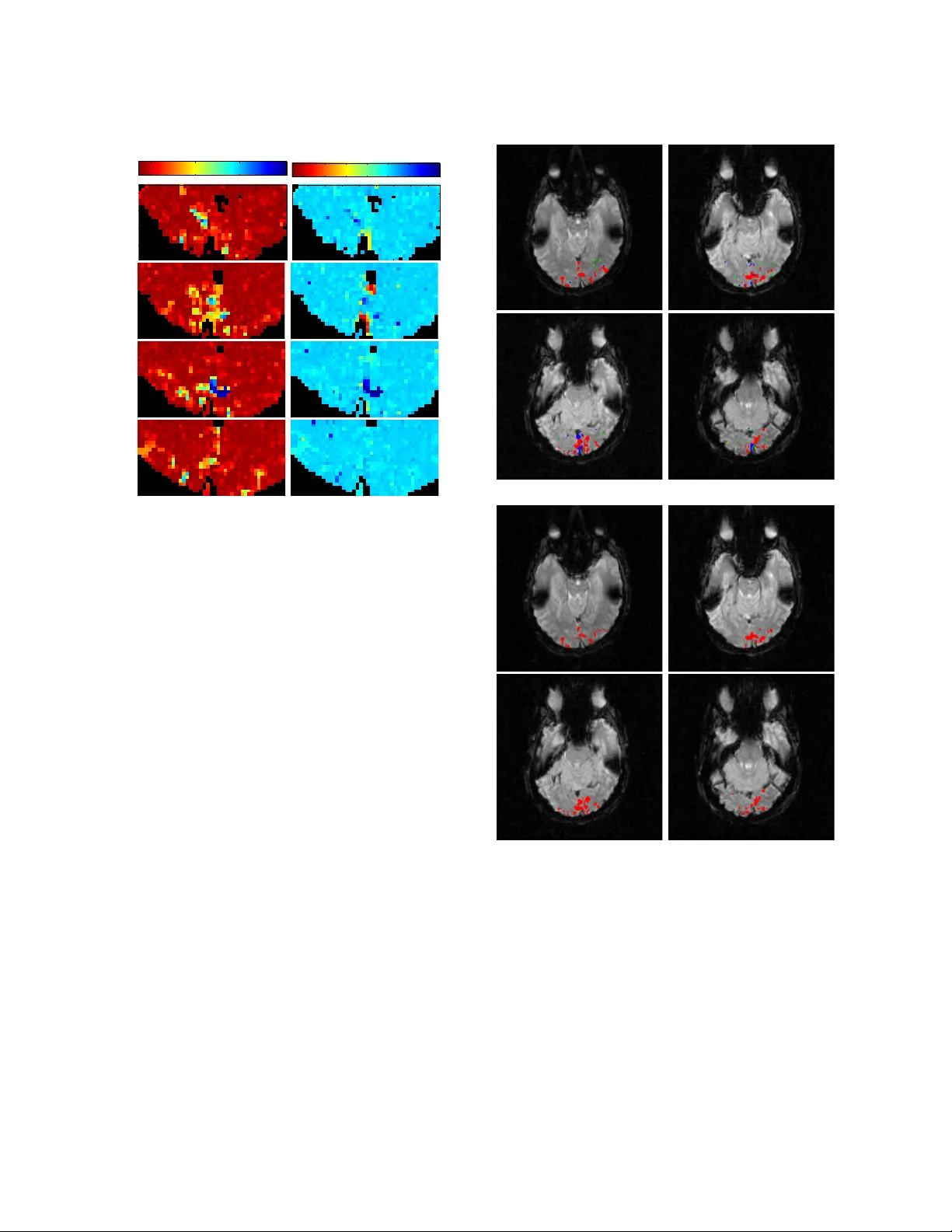
Lo w Dimensional Em b edding of fMRI datasets ? Xilin Shen, a F ran¸ cois G. Mey er a , ∗ a Dep artment of Ele ctric al Engine ering, University of Color ado at Boulder Abstract W e prop ose a no vel metho d to embed a functional magnetic resonance imaging (fMRI) dataset in a low-dimensional space. The em b edding optimally preserv es the lo cal functional coupling betw een fMRI time series and provides a lo w-dimensional coordinate system for detecting activ ated vo xels. T o compute the embedding, w e build a graph of functionally connected vo xels. W e use the commute time, instead of the geo desic distance, to measure functional distances on the graph. Because the commute time can b e computed directly from the eigen vectors of (a symmetric v ersion) the graph probability transition matrix, w e use these eigenv ectors to embed the dataset in low dimensions. After clustering the datasets in lo w dimensions, coherent structures emerge that can be easily interpreted. W e p erformed an extensive ev aluation of our metho d comparing it to linear and nonlinear techniques using syn thetic datasets and in vivo datasets. W e analyzed datasets from the EBC competition obtained with sub jects interacting in an urban virtual realit y environmen t. Our exploratory approac h is able to detect independently visual areas (V1/V2, V5/MT), auditory areas, and language areas. Our method can b e used to analyze fMRI collected during “natural stim uli”. Key wor ds: fMRI, Laplacian eigenmaps, embedding, natural stimuli. 1. In tro duction A t a microscopic level, a large n um b er of in ternal v ariables asso ciated with v arious ph ysical and ph ys- iological phenomena con tribute to dynamic c hanges in functional magnetic resonance imaging (fMRI) datasets. FMRI pro vides a large scale (as compared to the scale of neurons) measurement of neuronal activit y , and w e exp ect that many of these v ari- ables will b e coupled resulting in a low dimensional set for all p ossible conﬁgurations of the activ ated fMRI signal. W e assume therefore that activ ated fMRI time series can b e parametrized b y a small n umber of v ariables. This assumption is consisten t ? Submitted to Neuroimage, Sep. 2007. Revised Jan. 2008. ∗ Corresponding author. Email addr ess: fmeyer@Colorado.Edu (F ran¸ cois G. Meyer). URL: ece.colorado.edu / ∼ fmeyer (F ran¸ cois G. Meyer). with the usage of low dimensional parametric mo d- els for detecting activ ated v oxels (P etersson et al., 1999). This assumption is also consisten t with the empirical ﬁndings obtained with principal compo- nen ts analysis (PCA) and indep enden t comp onen ts analysis (ICA) (B.B.Bisw al and Ulmer, 1999; McK- eo wn et al., 2003), where a small num b er of compo- nen ts are suﬃcien t to describ e the v ariations of most activ ated temp oral patterns. Both PCA and ICA mak e v ery strong assumptions ab out the compo- nen ts: orthogonality and statistical indep endence, resp ectiv ely . Such constrain ts are conv enien t math- ematically but hav e no ph ysiological justiﬁcation, and complicate unnecessarily the in terpretation of the comp onen ts (F riston, 1998). A second limitation of PCA and ICA is that both metho ds only pro vide a linear decomposition of the data (F riston, 2005). There is no ph ysiological reason wh y the fMRI signal should be a linear com bination of eigen-images or Preprint submitted to Elsevier 22 October 2018 eigen-time series. In practice, the ﬁrst comp onents iden tiﬁed by PCA are often related to physiological artifacts (e.g. breathing), or coherent sp on taneous ﬂuctuations (Raichle and Mintun, 2006). These ar- tifacts can b e responsible for most of the v ariabilit y in the dataset. Stimulus triggered c hanges, whic h are muc h more subtle, rarely appear among the ﬁrst comp onen ts. The con tribution of this pap er is a nov el ex- ploratory metho d to construct an optimal coordi- nate system that reduces the dimensionalit y of the dataset while preserving the functional connectiv- it y b et w een v oxels (Sp orns et al., 2000). First, we deﬁne a distance b et ween time series that quan- tiﬁes the functional coupling (F ox et al., 2005), or connectivity b etw een the corresponding v o xels. W e then construct an embedding that preserv es this functional connectivit y across the entire brain. After em b edding the dataset in a lo wer dimen- sional space, time series are clustered in to coheren t groups. This new parametrization results in a clear separation of the time series in to: (1) response to a stim ulus, (2) coheren t ph ysiological signals, (3) ar- tifacts, and (4) background activity . W e p erformed an extensiv e ev aluation of our metho d comparing it to linear and nonlinear techniques using synthetic datasets and in vivo datasets. 2. Metho ds 2.1. Overview of our appr o ach Our goal is to ﬁnd a new parametrization of an fMRI dataset, eﬀectiv ely replacing the time series b y a small set of features, or co ordinates, that facili- tate the iden tiﬁcation of task-related hemo dynamic resp onses to the stimulus. The new co ordinates will also be able to rev eal the presence of physical or ph ysiological pro cesses that hav e an in trinsic low dimension. Suc h processes can be describ ed with a small n umber of parameters (dimensions) in an appropriate representation (set of basis functions). These time series should b e contrasted with noise time series that ha ve a very diﬀuse representation in any basis. Example of such low-dimensional pro- cesses include task-related hemo dynamic resp onses, non-task-related ph ysiological rhythms (breathing and heart beating motion). W e exp ect that only a small fraction of all time series will ha ve a low- dimensional represen tation. The remaining time se- ries will b e engaged in a sp on taneous in trinsic activ- it y (Raichle and Mintun, 2006). W e call these time series b ackgr ound time series . As sho wn in our ex- p erimen ts, background time series are more com- plex, and cannot b e well approximated with a small n umber of parameters. W e no w introduce some notations that will b e used throughout the paper. Let X denote an fMRI dataset comp osed of T scans, each comprised of N v oxels, which is represented as a N × T matrix, X =      x 1 (1) · · · x 1 ( T ) . . . . . . . . . x N (1) · · · x N ( T )      . (1) Ro w i of X is the time series x i = [ x i (1) , · · · , x i ( T )] generated from vo xel i . Column j is the j th scan unrolled as a 1 × N vector. In this work, we regard x i as a p oint in R T , with T co ordinates. W e seek a new parametrization of the dataset that optimally preserves the lo cal functional coupling b e- t ween time series. Most metho ds of reduction of di- mensionalit y used for fMRI are linear: each x i is pro- jected on to a set of comp onen ts φ k . The resulting co eﬃcien ts < x i , φ k >, k = 0 , · · · , K − 1 serve as the new co ordinates in the low dimensional representa- tion. Ho w ever, in the presence of nonlinearit y in the organization of the x i in R T , a linear mapping may distort lo cal functional correlations. This distortion will make the clustering of the dataset more diﬃcult. Our exp erimen ts with in vivo data conﬁrm that the subsets formed by the low-dimensional time series ha ve a nonlinear geometry and cannot be mapp ed on to a linear subspace without signiﬁcant distortion. W e propose therefore to use a nonlinear map Ψ to represen t the dataset X in low dimensions. Because the map Ψ is able to preserve the lo cal functional coupling b etw een v oxels, low dimensional coheren t structures can easily b e detected with a clustering algorithm. Finally , the temp oral and the spatial pat- terns asso ciated with eac h cluster are examined and the cluster that corresp onds to the task-related re- sp onse is identiﬁed. In summary , our approac h in- cludes the following three steps: (i) Low dimensional embedding of the dataset; (ii) Clustering of the dataset using the new pa- rameterization; (iii) Identiﬁcation of the set of activ ated time se- ries. 2 Fig. 1. The netw ork of functionally correlated vo xels, repre- sented by a graph, encodes the functional connectivity b e- tw een time series. 2.2. The c onne ctivity gr aph: a network of functional ly c orr elate d voxels In order to construct the nonlinear map Ψ w e need to estimate the functional correlation b et ween vo x- els. W e characterize the functional correlation b e- t ween v oxels with a netw ork. Similar net works ha ve b een constructed to study functional connectivity in (Ac hard et al., 2006; Caclin and F onlupt, 2006; Egu ´ ıluz et al., 2005; F o x et al., 2005; Sp orns et al., 2000). W e represent the netw ork by a graph G that is constructed as follo ws. The time series x i origi- nating from v oxel i b ecomes the node (or v ertex) x i of the graph 1 . Edges b et ween v ertices quantify the functional connectivit y . Eac h node x i is connected to its n n nearest neighbors according to the Eu- clidean distance b et ween the time series, k x i − x j k = ( P T t =1 ( x i ( t ) − x j ( t )) 2 ) 1 / 2 (Fig. 1). The weigh t W i,j on the edge { i, j } quantiﬁes the functional pro xim- it y b et ween vo xels i and j and is deﬁned by W i,j = ( e −k x i − x j k 2 /σ 2 , if x i is connected to x j , 0 otherwise. (2) The scaling factor σ modulates the deﬁnition of pro ximity measured b y the weigh t (2). If σ is v ery large, then for all the nearest neigh b ors x j of x i , w e ha ve W i,j ≈ 1 (see (2)), and the transition proba- bilit y is the same for all the neighbors, P i,j = 1 /n n . 1 W e sligh tly abuse notation here: x i is a time series, as w ell as a no de on the graph. This choice of σ promotes a very fast diﬀusion of the random walk through the dataset, and blurs the distinction b etw een activ ated and background time series. On the other hand, if σ is extremely small, then P i,j = 0 for all the neighbors such that k x i − x j k > 0. Only if the distance betw een x i and x j is zero (or very small) the transition probabilit y is non zero. This choice of σ accen tuates the diﬀer- ence b etw een the time series, but is more sensitiv e to noise. In practice, we found that the univ ersal c hoice σ = n × min i 1 / √ 1 − λ 3 > · · · 1 / √ 1 − λ N . W e can therefore ne- glect φ k ( j ) / √ 1 − λ k in (7) for large k , and reduce the dimensionality of the em b edding by using only the ﬁrst K co ordinates. Finally , we deﬁne the map Ψ from R T to R K , x i 7→ Ψ( x i ) = 1 √ π i " φ 2 ( i ) √ 1 − λ 2 , · · · · · · , φ K +1 ( i ) p 1 − λ K +1 # T . (8) The low dimensional parametrization (8) pro vides a go od approximation when the sp ectral gap λ 1 − λ 2 = 1 − λ 2 , is large. The construction of the embedding is summarized in Fig. 3. Unlike PCA which gives a set of v ectors on whic h to pro ject the dataset, the em b edding (8) directly yields the new co ordinates for eac h time series x i . The new co ordinates of x i are giv en by concatenating the i th co ordinates of φ k , k = 2 , · · · , K + 1. The ﬁrst eigenv ector φ 0 is constan t and is not used. What is the c onne ction to PCA ? Because each φ k is also an eigenv ector of the graph Laplacian, L = I − D 1 2 PD − 1 2 , it minimizes the “dis- tortion” induced by φ and measured by the Rayleigh ratio (Belkin and Niyogi, 2003), min φ , k φ k =1 P i,j W i,j ( φ ( i ) − φ ( j )) 2 P i d i φ 2 ( i ) , (9) where φ k is orthogonal to the previous eigen vector { φ 0 , φ 1 , · · · , φ k − 1 } . The gradien t of φ at the v ertex x i on the graph can b e computed as a linear com- bination of terms of the form ( φ ( i ) − φ ( j )), where j and i are connected. Therefore the numerator of the Rayleigh ratio (9) is a weigh ted sum of the gra- dien ts of φ at all no des of the graph, and quantiﬁes the av erage lo cal distortion created b y the map φ . A function that minimizes (9), will still introduce some global distortions. Only an isometry will preserve all distances b et ween the time series, and the isometry whic h is optimal for dimension reduction is given b y PCA. How ever, as sho wn in the experiments, the ﬁrst PCA components are usually not able to cap- ture the nonlinear structure formed by the set of time series. As a result, PCA fails to reveal the orga- nization of the dataset in terms of lo w dimensional activ ated time series and bac kground time series. Thirion and F augeras (2003) hav e used kernel PCA to analyze the distributions of the coeﬃcients of a mo del ﬁtted to fMRI time series. A blo c k design fMRI dataset from a macaque monkey is studied. By visual inspection, the authors sho w that their metho d can organize the coeﬃcients according to the relative strength of the activ ation. The eigen- v ectors of the Laplacian ha ve also b een used to con- struct maps of spectral coherence of fMRI data in (Thirion et al., 2006). How many new c o or dinates do we ne e d ? W e can estimate K , the num b er of coordinates in the embedding (8), b y calculating the n umber of φ k needed to reconstruct the low dimensional struc- tures present in the dataset. As opp osed to PCA, the em b edding deﬁned b y (8) is not designed to mini- mize the reconstruction error, it only minimizes the a verage lo cal distortion (9). Nevertheless, w e can tak e adv antage of the fact that the eigen vectors { φ k } constitute an orthonormal basis for the set of func- tions deﬁned on the v ertices of the graph (Chung, 1997). In particular, w e mak e the trivial observ ation that the scan at time t , x ( t ) = [ x 1 ( t ) , · · · , x N ( t )] T , is a function deﬁned on the nodes of the graph: x ( t ) at node x i is the v alue of the fMRI signal at vo xel i , x i ( t ). W e can therefore expand x ( t ) using the φ k , 5 x ( t ) = K X k =1 < x ( t ) , φ k > φ k + N X k = K +1 < x ( t ) , φ k > φ k = ˆ x K ( t ) + r ( t ) , where ˆ x K ( t ) = P K k =1 < x ( t ) , φ k > φ k is the ap- pro ximation to the t th scan using the ﬁrst K eigen- v ectors, and r ( t ) is the residual error. W e can com- pute a similar approximation for all the scans ( t = 1 , · · · , T ), and compute the temp oral a v erage of the relativ e approximation error at a given vo xel i , ε i ( K ) = P T t =1 ( x i ( t ) − ˆ x i K ( t )) 2 P T t =1 x 2 i ( t ) . (10) Finally , one can compute the a verage of ε i ( K ) ov er all a group of vo xels in the same functional area R , ε R ( K ) = ( P i ∈R ε i ( K )) / |R| . W e exp ect ε R ( K ) to deca y fast with K if the time series within R are w ell appro ximated b y φ 1 , · · · , φ K . In practice, for each region R we ﬁnd K R after which ε R stops ha ving a fast decay . W e then c ho ose K the num b er of co ordinates to b e the largest K R among all regions R . Examples are shown in Fig. 9-right, where K is c hosen at the “knee” of the curves ε R ( K ). 2.5. k -me ans clustering The map Ψ deﬁned b y (8) pro vides a set of new co ordinates, Ψ( x i ), for eac h x i . W e cluster the set { Ψ( x i ) , i = 1 , · · · , N } into a small n umber of coher- en t structures and a large background comp onen t. W e use a v ariation of the k -means clustering algo- rithm for this task. The low dimensional parameteri- zation of the dataset usually has a “star” shap e (Fig. 4-left), where the out-stretching “arms” of the star are related to activ ated time s eries or strong phys- iological artifacts, and the cen ter blob corresp onds to bac kground activity . Our goal is to segment eac h of the “arms” from the cen ter blob. W e pro ject all the Ψ( x i ) on a unit sphere centered around the ori- gin (Fig. 4-righ t). W e then cluster the pro jections on the sphere: the distance betw een t wo points on the sphere is measured by their angle. The center comp onen t (shown in blac k in Fig. 4-left) is usu- ally spread all o ver the sphere, and is mixed with the branc hes (Fig. 4-right). The time series from the bac kground comp onen t can b e separated from the other time series b y measuring the distance of Ψ( x i ) to the origin (Fig. 4-left). The num b er of clusters Fig. 4. Left: low dimensional em b edding of the dataset an- alyzed in section 3.2. Each dot i is Ψ( x i ), the image of the time series x i through the mapping Ψ. Right: the Ψ( x i ) are pro jected on the sphere, and the pro jections are clustered on the sphere. can be chosen to b e equal to K + 1. This c hoice is based on exp erience that each eigenv ector (eac h dimension) will con tribute to an independent arm, and the background time series will contribute to the last cluster. This choice ma y o ver-segmen t the dataset. This is usually ob vious from the visual in- sp ection scatter plot, and the corresponding spatial maps. W e iterativ ely reﬁne th e estimate of the num- b er of clusters, by merging small clusters at eac h iteration. 3. Results In this section we describe the results of exp eri- men ts conducted on synthetic and in-vivo datasets. W e construct the embedding according to the algo- rithm describ ed in Fig 3, and the clustering algo- rithm, describ ed in section 2.5, divides the em b ed- ded dataset into coherent groups. W e interpret the coheren t structures in terms of a task-related hemo- dynamic resp onse, and physiological artifacts. V ox- els that correspond to task-related activ ation are iden tiﬁed and activ ation maps are generated accord- ingly . W e ev aluate our approach using t wo diﬀer- en t criteria. First, w e compare the parameterization created b y our approach with the parametrization pro duced by PCA. The comparison is based on 6 Fig. 5. Left: synthetic brain: activ ation (white), non-activ a- tion (gray), outside the brain (black). Right: stimulus time series. our ability to identify and extract well deﬁned struc- tures from the new parameterization. Our second criterion is the comparison of the activ ation maps obtained with our approac h with the ones gener- ated b y the General Linear Mo del (GLM). Five datasets are selected for the analysis: a synthetic dataset, a block design dataset, an even t-related dataset, and tw o datasets from the EBC competi- tion Universit y of Pittsburgh (2007). 3.1. Synthetic data The syn thetic datasets were designed b y blend- ing activ ation into background, non activ ated, time- series that were extracted from a real in vivo dataset (describ ed in section 3.2). W e discarded time series exhibiting large v ariance. Activ ated time-series were constructed b y adding an activ ation pattern f ( t ) to the background time series. The activ ation pattern f ( t ) was obtained b y con volving the canonical hemo- dynamic ﬁlter h ( t ) used in SPM (F riston, 2005) h ( t ) = α  t d 1  a 1 e − ( t − d 1 ) /b 1 − c  t d 2  a 2 e − ( t − d 2 ) /b 2 , (11) with the stim ulus time-series g ( t ) (Fig. 5-left). The t wo parameters α and b 1 w ere randomly distributed according to tw o uniform distributions, on [0 . 8 , 1 . 2] and on [5 , 10] resp ectiv ely . The other parameters w ere ﬁxed and c hosen as follows, a 1 = 6 , a 2 = 12 , b 2 = 0 . 9 , and c = 0 . 35. By v arying b 1 and α indep enden tly , we generated a family of hemody- namic resp onses with diﬀeren t peak dispersions and scales. W e generated 20 indep endent realizations according to this design. Eac h dataset consisted of a white disk of activ ated vo xels inside a circular gra y brain of background vo xels (Fig. 5-left). Black v oxels w ere in the air. There were altogether 1067 v oxels inside the circular brain, with 97 activ ated Fig. 6. Activ ated (red) and background (blac k) time se- ries pro jected on the ﬁrst tw o PCA components (left), and parametrized by Ψ (right). Fig. 7. Left: clustering of { Ψ( x i ) , i = 1 , · · · , N } into 2 clus- ters: activ ated (red) and background (black). Right: acti- v ated (white) and bac kground (gray) pixels. v oxels, (9% activ ation). Fig. 6-left shows the pro- jections on the ﬁrst t wo principal axes of the 1067 time series of one realization. The pro jections are color-co ded according to their status: activ ated (red diamond) and background (black circle). The pa- rameterization giv en by our approac h is shown in 6-righ t. W e used only K = 2 coordinates in (8) for Ψ. Activ ated time series are distributed along a thin strip that extends out ward from the main cluster. This low dimensional structure is compact and easy to identify . In comparison, the tw o dimen- sional represen tation given by PCA (Fig. 6-left) is less conspicuous: activ ated time series (red) ov erlap with background time series (black). After em b ed- ding the dataset in to tw o dimensions, the dataset is partitioned into t wo clusters. Fig. 7-left shows the re- sult of clustering: the lab els (red for activ ated, black for background) are based on the clustering only . The corresponding activ ation map is sho wn in Fig. 7-righ t. W e compared our algorithm with a linear mo del equipp ed with the perfect kno wledge of the hemo dynamic resp onse h ( t ) (with b 1 = 1 and α = 1). A Student t -test was applied to the regression co eﬃcien t to test its signiﬁcance, and vo xels with a p -v alue smaller than a threshold w ere considered activ ated. Fig. 8 provides a quantitativ e comparison 7 0 0.001 0.003 0.005 0.007 0.009 0.011 0 0.1 0.2 0.3 0.4 0.5 0.6 0.7 0.8 0.9 1 False Positive Rate True Positive Rate GLM Laplacian Fig. 8. R OC curves: comparison of our approach to the GLM. of our approach with the linear mo del using a re- ceiv er op erator c haracteristic (ROC) curve. The true activ ation rate (one minus the type I I error) is plotted against the t yp e I error (false alarm rate). The R OC curve was computed ov er 20 trials. Eac h trial included diﬀeren t activ ation strengths α . In this experiment, the linear mo del has access to an oracle, in the form of the perfect kno wledge of the hemo dynamic response h ( t ), and should therefore p erform very w ell. In fact, if the noise added to f ( t ) w ere to b e white, we kno w from the matc hed ﬁlter theorem that the linear mo del w ould pro vide the optimal detector. Here,the noise is extracted from the data, and is probably not white (Bullmore et al., 2001). As shown in Fig. 8, our approach performs as w ell as the GLM for a type I error in the range [0.003,0.009]. At lo w t yp e I error, our approach misses activ ations. 3.2. In vivo data I: blo ck design dataset W e apply our tec hnique to a blo c k design dataset that demonstrates activ ation of the visual cortex (T anab e et al., 2002). A ﬂashing c heck erb oard im- age w as presen ted to a sub ject for 30 seconds, and a blank image was presented for the next 30 seconds. This alternating cycle was rep eated four times. Im- ages w ere acquired with a 1 . 5T Siemens MAGNE- TOM Vision equipp ed with a standard quadrature head coil and an echoplanar subsystem (TR = 3s, xy dimension: 128 × 128, vo xel size = 1 . 88 × 1 . 88 × 3mm, 12 contiguous slices). Eight y images were obtained. W e analyze a v olume that contains the calcicarin cortex (Bro dman areas 17) (Fig. 13). There are al- together 3084 intracranial time series in the volume. The linear trend of eac h time series is remo ved. Fig. 9-left displays the image of the time series by the 2 4 6 8 10 12 0.5 0.55 0.6 0.65 0.7 0.75 0.8 0.85 0.9 0.95 1 Residual Energy Cluster III Cluster I Background Cluster Cluster II Fig. 9. Three-dimensional embedding: { Ψ( x i ) , i = 1 , · · · , 3084 } : cluster I (red), cluster II (blue), cluster II I (green), and background (black). Time series marked by a circle are shown in Fig. 11. Right: residual error ε R ( K ) as a function of the num b er of coordinates K . Fig. 10. Low dimensional em b edding obtained b y PCA (left), and ISOMAP (right). A B C Fig. 11. Time series from the cluster I ( A ), cluster I I ( B ), and cluster I II ( C) . em b edding, Ψ( x i ) , i = 1 , · · · , 3084. The time series are color-co ded according to the result of the cluster- ing. The dataset is partitioned into four clusters. F or comparison purp oses, we show the em b edding gen- erated b y ISOMAP (T enenbaum et al., 2000) (Fig. 10-left), and the embedding obtained by pro jecting the time series on the ﬁrst three PCA axes (Fig. 10-righ t). ISOMAP makes it possible to reconstruct a low dimensional nonlinear structure embedded in high dimension. The algorithm computes the 8 11 beltrami: slice−4 eigenvector−2 5 10 15 20 5 10 15 20 25 30 35 40 −0.15 −0.1 −0.05 0 beltrami: slice−4 eigenvector−3 5 10 15 20 5 10 15 20 25 30 35 40 −0.1 −0.05 0 0.05 0.1 0.15 0.2 10 9 8 φ 2 φ 3 Fig. 12. Eigenv ectors φ 2 and φ 3 visualized as images. pairwise geodesic distance betw een an y t wo p oin ts in the dataset, and uses m ultidimensional scaling to em b ed the dataset in lo w dimension. As explained in section 2.3, the geodesic distance is not appropriate for fMRI data that are v ery noisy . F or this reason an em b edding based on commute time is more robust. The represen tation given by PCA and ISOMAP , sho wn in Fig. 10 left and right, are less conspicuous than the represen tation obtained b y our approac h. No low dimensional structures are apparen t in these t wo plots. The plot of the residual error (Fig. 9- righ t) indicates that eigenv ectors φ 2 and φ 3 create the largest drop in the residual energy , and should b e the most useful. W e use K = 3 co ordinates: φ 2 , φ 3 and φ 4 to em b ed the dataset. In order to in terpret the role of the clusters, we select several time series from each cluster (identiﬁed b y circle in the scat- ter plot in Fig. 9) and plot them in Fig. 11. The time series from the red cluster (Fig. 11- A ) are typ- ical hemo dynamic resp onses to a p eriodic stimulus. The time series at the tip of the red cluster, marked b y a red circle, is the red curv e in Fig. 11- A . It is the strongest activ ation pattern. Times series in the middle of the red cluster (blue and black circles) ex- hibit weak er activ ation (blue and black curv es). W e in terpret cluster I as v oxels activ ated by the stim- ulus. The em b edding has organized the time series according to the strength of the activ ation: strong activ ation at the tip and weak activ ation at the base Fig. 13. T op two rows: vo xels are color-co ded according to the cluster color (except for the background cluster). W e in- terpret cluster I (red) as v oxels in the visual cortex recruited by the stim ulus. Bottom tw o rows: activ ation maps obtained using the linear regression mo del ( p = 0 . 001). of the branch (close to the background activit y). The time series from the blue cluster hav e a high frequency (Fig. 11- B ), and are grouped together in- side the brain (Fig. 13). These time series could b e related to non-task related ph ysiological resp onses, suc h as a pulsating vein. Finally , the time series from the green cluster are less structured (Fig. 11), and are scattered across the region of analysis (Fig. 13). W e were not able to interpret the physiological 9 role of these time series. So what do the eigenve ctors lo ok like ? As explained in section 2.3, we consider the eigen- v ectors φ k to be functions of the no des i of the graph. W e can therefore represen t φ k as an image: eac h v oxel x i is color-co ded according to the v alue of φ k ( i ). The ma jorit y of the v alues of φ 2 are p ositiv e (deep red, in Fig. 12-left). A few vo xels take neg- ativ e v alues (yello w and cyan in Fig. 12-left). The no dal lines (where φ 2 c hanges sign) are lo calized around the area of activ ation in the visual cortex. W e can chec k in Fig. 9 that the activ ated time series (red cluster) ha ve a negative φ 2 co ordinate. In fact, φ 2 is kno wn as the Fiedler vector (Chung, 1997) and is used to optimally split a dataset into t wo parts. (Fig. 12). W e computed the activ ation map obtained using a GLM. The regressor is computed b y con volving the haemodynamic response deﬁned b y (11) with the exp erimen tal paradigm. The acti- v ation map (thresholded at p = 0 . 001) is shown in Fig. 13, and is consisten t with the activ ation maps obtained by our approach. 3.3. In vivo data II: event-r elate d dataset W e apply our metho d to an even t-related dataset. Buc kner et al. (2000) used fMRI to study age-related c hanges in functional anatom y . The sub jects w ere instructed to press a key with their right index ﬁnger up on the visual stim ulus onset. The stimulus lasted for 1 . 5s. F unctional images were collected using a Siemens 1 . 5-T Vision System with an asymmetric spin-ec ho sequence sensitive to BOLD contrast (vol- ume TR = 2 . 68s, xy dimension: 64 × 64, v oxel size: 3 . 75 × 3 . 75mm, 16 contiguous axial slices). Each run consists of 128 TRs. F or every 8 images, the sub jects w ere presen ted with one of the t wo conditions: (i) the one-trial condition where a single stimulus was presen ted to the sub ject, and (ii) the two-trial condi- tion where tw o consecutive stim uli w ere presented. The in ter-stimulus interv al of 5 . 36 s. w as suﬃcien tly large to guaran tee that the o verall resp onse w ould b e ab out twice as large as the resp onse to the one- trial condition. W e analyzed one run. After discard- ing the ﬁrst and last four scans, the run included 15 trials (8 one-trial and 7 two trial conditions) of 8 temp oral samples. Time series from the one-trial and two-trial conditions w ere av eraged separately . Therefore, each vo xel ga ve rise to tw o av erage time series of 8 samples. The linear trend was remov ed Fig. 14. Three-dimensional em b edding. Left: one-trial (blue) and two-trial (red) conditions are w ell separa ted. Righ t: clus- ter I (blue), cluster I I (red) and background (green). Time series marked by a circle are shown in Fig. 16. Fig. 15. Low dimensional em b edding obtained b y PCA (left), and ISOMAP (right). One-trial condition (blue) and two– trial condition (red) are mingled. 10 from all av erage time series. The results published in (Buc kner et al., 2000) show activ ation in the visual cortex, motor cortex, and cereb ellum. W e fo cus our analysis on four contiguous axial slices (7, 8, 9 and 10) that extend from the sup erior caudate n ucleus to the midlevel diencephalon. W e extract a region (1025 in tracranial vo xels) that extends from the oc- cipital posterior horn of the lateral ven tricles un til the end of the o ccipital lobe. The total num b er of time series included in our analysis is 2050: t wo time series ( one-trial and two-trial conditions) of T = 8 samples for each vo xel. Emb e dding the dataset in 3 dimensions W e display in Fig. 14-left the 2050 time series af- ter embedding the dataset in three dimension. The one-trial condition time series (blue) form a blob at the center. The two-trial (red) conditions time series form a “V” (Fig. 14-right). Both branches of the “V” are nearly one dimensional and are aligned with φ 2 and φ 4 . The branch aligned with φ 2 also includes one-trial condition time series at the base of the branc h. The branc h aligned with φ 4 con tains only two-trial condition time series. The dataset w as par- titioned in to three clusters (Fig. 14-righ t). W e com- pare our em b edding to the embedding generated b y ISOMAP (Fig. 15-left) and PCA (Fig. 15-right). No lo w-dimensional structures emerge from the repre- sen tations given b y PCA or ISOMAP , and two-trial and one-trial time series are mixed together. The eigen vectors φ 2 and φ 4 create the largest drop in the residual energy , and are the most useful co ordinates. W e use K = 3 co ordinates: φ 2 , φ 3 and φ 4 to em b ed the dataset. T o determine the role of the clusters, w e select three groups of four time series (identiﬁed b y circles in Fig. 14-right) and we plot them in Fig. 16. Time series from cluster I all ha ve an abrupt dip at t = 7. The corresp onding vo xels are lo cated along the b order of the brain (Fig. 17). The original time series (b efore av eraging) suﬀer from a sudden drop at time 95, which could be caused by a motion arti- fact, that aﬀects the av erage time series. There are t wo groups of time series selected from cluster I I: t wo two-trial condition time series lo cated at the tip of the branc h, and t wo one-trial condition time series lo cated at the border with the bac kground cluster. Time series from cluster I I hav e a shap e similar to an hemo dynamic resp onse (Fig. 16-B and C), and the corresp onding v oxels are lo cated in the visual cortex (Fig. 17). Therefore, we hypothesize that cluster I I con tains times series recruited b y the stimulus. In- terestingly , the embedding has organized the time series along the branch A B C Fig. 16. F our representativ e time series from cluster I ( A ) , cluster I I with one-trial condition ( B ), and from cluster I I with two-trial condition ( C) . of cluster I I according to the strength of the activ a- tion: from two-trial condition (strong resp onse) at the tip, to one-trial condition (weak resp onse) at the stem (close to the background time series). This is a remark able result since no information ab out the stim ulus, or the t yp e of trial w as provided to the algorithm. Fig. 17 shows the lo cation of the v oxels corresp onding to the time series of cluster I (blue) and I I (red). F or comparison purposes w e computed the activ ation map obtained using the GLM. The a veraged time series from the two-trial condition are used for the regression analysis. W e use the hemo dy- namic resp onse function deﬁned by (Dale and Buc k- ner, 1997), h ( t ) = (( t − δ ) /τ ) 2 e ( t − δ ) /τ , where δ = 2 . 5, τ = 1 . 5. The regressor was giv en by g ( t ) = h ( t ) ∗ s ( t ), where s ( t ) is the stim ulus time series. W e thresholded the p -v alue at p = 0 . 005, and the activ a- tion maps are sho wn in Fig.17. The activ ation maps constructed by our approach are consisten t with the maps obtained with a GLM. 3.4. Complex natur al stimuli W e demonstrate here that our metho d can b e used to analyze fMRI datasets collected in natu- ral environmen ts where the sub jects are b ombarded with a m ultitude of uncontrolled stim uli that can- not be quantiﬁed (Golland et al., 2007; U.Hason et al., 2004; Haynes and Rees, 2006; Malinen et al., 2007; Mey er and Stephens, 2008). During such ex- p erimen ts, the sub jects are submitted to an abun- dance of concurren t sensory stimuli, whic h mak es the analysis with inferential metho ds imp ossible. 11 Fig. 17. T op tw o rows: activ ation maps: cluster I (blue) , cluster II (red). Bottom t wo ro ws: activ ation maps obtained using the linear regression mo del ( p = 0 . 005). Exploratory techniques can help unra vel the dif- feren t neural processes in volv ed during the exp eri- men ts (Malinen et al., 2007). Unlike ICA, our ap- proac h does not p osit the existence of a mixture mo del. Our approach merely explores the connec- tivit y in the dataset, and prop oses a new parame- terization that preserves connectivity . The Exp erience Based Cognition comp etition (EBC) (Universit y of Pittsburgh, 2007) oﬀers an opp ortunit y to study complex resp onses to natural en vironments. The EBC datasets comprise three 20-min ute runs (704 TRs in each run) of sub jects in teracting in an urban virtual reality environ- men t. Sub jects were audibly instructed to complete three search tasks in the environmen t: lo oking for w eap ons (but not to ols) taking pictures of peo- ple with piercing (but not others), or picking up fruits (but not vegetables). The data w as collected with a 3T EPI scanner (TR = 1 . 75s, xy dimension: 64 × 64, vo xel size = 3 . 28 × 3 . 28mm, 34 slices with a thickness of 3 . 5mm). W e analyze the second runs of sub jects 14 and 13. F or each sub ject, the matrix X is comp osed of N = 4843 intra-cranial v oxels at T = 704 TRs. W e ﬁrst remov e the non regionally sp eciﬁc v ariance captured by the ﬁrst eigenmo des of a singular v alue decomposition of the dataset. W e then compute φ k , k = 2 , · · · 10 using n n = 100 and σ = 2 × min i

Original Paper

Loading high-quality paper...

Comments & Academic Discussion

Loading comments...

Original Paper

Related Papers

Comments & Academic Discussion

Leave a Comment