A Central Limit Theorem for the SNR at the Wiener Filter Output for Large Dimensional Signals

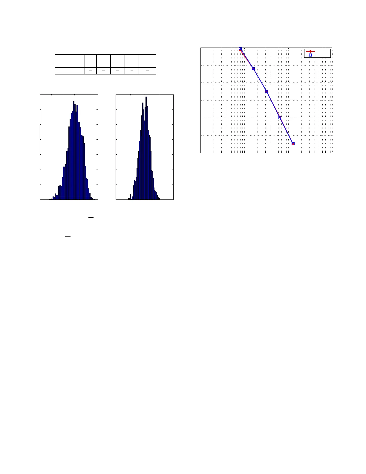
A CENTRAL LIMIT THEOREM FOR THE SNR A T THE WIENER FIL TER OUTPUT FOR LARGE DIMENSIONAL SIGNALS Abla Kammoun (1) , Malika Khar ouf (2) , W alid Hachem (3) and J amal Najim (3) (1) ENST (France), (2) Casablanca Unive rsit y (Morocco), (3) CNRS/ ENST (France). (abla.kamm oun, malika.kharouf, walid.hach em, jamal.naj im@enst.fr) ABSTRA CT Consider the quadratic form β = y ∗ ( YY ∗ + ρ I ) − 1 y where ρ is a positiv e number , where y is a random vector and Y i s a N × K random matrix both having independent elements with dif fer- ent variances, and where y and Y are ind ependent. Such qu adratic forms represent the Si gnal to Noise Ratio at the o utput of the linear W iener receiv er for multi dimensional signals fr equently encoun- tered in wireless communications and in array processing. Using well kno wn results of Random Matrix Theory , the quadratic form β can be approx imated with a kno wn deterministic r eal number ¯ β K in the asymptotic reg ime where K → ∞ and K/ N → α > 0 . This paper ad dresses the problem of c onv ergence of β . More specifically , it is sho wn here that √ K ( β − ¯ β K ) behav es for large K like a Gaus- sian random v ariable which variance is prov ided. Index T erms — Antenna Arrays, CDMA, Central Limit Theo- rem, MC-CDMA, Random Matrix Theory , Wien er F iltering. 1. INTRODUCTION Consider the N dimensional receiv ed si gnal r = Σs + n where s = [ s 0 , s 1 , . . . , s K ] T is the t ransmitted complex vector si g- nal wit h size K + 1 satisfying E ss ∗ = I K +1 , matrix Σ represents the “channel” in the wide sense and n i s the independent A WGN with co varianc e matrix E nn ∗ = ρ I N > 0 . In this article, we are in- terested i n the performa nce of the l inear Wiener estimate (also c alled LMMSE for Linear M inimum Mean Squared Error estimate) of sig- nal s 0 . Among the variou s performance index es, we shall focus on the Signal to Noise Ratio (SNR) which can be e xpressed as follows: Partition the channel matrix as Σ = [ y Y ] , the n the Wiener estimate ˆ s 0 of s 0 writes ˆ s 0 = y ∗ ( ΣΣ ∗ + ρ I N ) − 1 r an d the associated SNR β K is giv en by: β K = y ∗ ( YY ∗ + ρ I N ) − 1 y . A popular t ool to address t his problem, widely used in multi dimen- sional signal processing and communication engineering, is repre- sented by the theory of Large Random Matrices: A ssume that Σ is random (in this case, β K becomes a conditional SNR) and l et N → ∞ with K/ N → α > 0 (d enoted in the sequel by “ K → ∞ ” for short). As amply shown in the literature, there are many st a- tistical models related to Σ for which there exists a deterministic sequence ¯ β K such that β K − ¯ β K → 0 almost surely (a.s.); this ap- proximation is generally defined as the solution of an implicit equa- tion. Bey ond the con vergen ce of the SNR, a natural practical and W ork partiall y funded by the French “ Fonds National de la Scienc e ”, A CI/NIM project number 205 (MALCOM). theoretical problem concerns the study of its fl uctuations (t hink for instance t o the outage probability ev aluations). Despite its interest, there are very few related art icles in t he lit erature. In this paper, we provid e a Central Limit Theorem (CL T) for β K as K → ∞ for a general model of matrix Σ : Assume that the N × ( K + 1) matrix Σ i s giv en by: Σ = 1 √ K [ σ nk W nk ] N,K n =1 ,k =0 (1) where ( σ 2 nk ; 1 ≤ n ≤ N ; 0 ≤ k . . . , K ) is a sequence of rea l num- bers called a v ariance profile and where the complex random v ari- ables W nk are independent and identically distributed (i.i.d.) with E W nk = 0 , E W 2 nk = 0 , and E | W nk | 2 = 1 . In this case, the quadratic form β K is giv en by: β K = 1 K w ∗ 0 D 1 / 2 0 ( YY ∗ + ρ I N ) − 1 D 1 / 2 0 w 0 (2) where w 0 = [ W 10 , W 20 , . . . , W N 0 ] T and D 0 is t he N × N diag- onal nonnegati ve matrix D 0 = diag ( σ 2 10 , . . . , σ 2 N 0 ) . An important special case that we shall describe carefully in the sequel is when the v ariance profil e is separ able , i.e σ 2 nk = d n ˜ d k . Among the many applications of the general model (1), l et us mention: • Multiple antenna transmissions with K + 1 antennas at the transmission side and N antennas at the reception side. Here we consider the tr ansmission model r = Ξs + n where Ξ = 1 √ K HP 1 / 2 , matri x H is a N × ( K + 1) random matrix with comple x Gaussian elements representing the ra- dio channel and P = d iag( p 0 , . . . , p K ) is the (determinis- tic) matrix of the powers giv en to the differe nt users. Write H = [ h 0 · · · h K ] , and assume the columns h k are indepen- dent, which is realistic when the transmitters are distant one from another . Let C k be the co variance matrix C k = E h k h ∗ k and l et C k = U k Λ k U k be a spectral decomposition of C k where Λ k = diag(( λ nk ) n =1 ,...,N ) is the matrix of eigen val- ues. If the eigen vector matrices U 0 , . . . , U K are all equal (note that sometimes they are all identified with the Fourier N × N matrix [1]), then one can sho w that matrix Ξ in- troduced abov e can be replaced with matri x Σ of Model (1) where the W nk are standard Gaussian iid and σ 2 nk = λ nk p k . In certain situations it is furthermore assumed that Λ 0 = · · · = Λ K = diag ( λ 1 , . . . , λ N ) : this is the well kno w n Kro- necke r model with correlations at reception. In our setting this model is accounted for by the separable variance profile case σ 2 nk = λ n p k . • CDMA transmissions on fl at fading channels. Here N i s the spreading factor , K + 1 is the number of users, and Σ = WP 1 / 2 (3) where W is t he N × ( K + 1) signature matrix assumed here to ha ve random i.i.d. elements with mean zero , variance 1 / N and where P = diag( p 0 , . . . , p K ) is th e users po wers matrix. In this case, the variance profile is sepa rable with d n = 1 and ˜ d k = K N p k . • MC-CDMA transmissions on frequency selectiv e channels. In the uplink, the matrix Σ is written: Σ = [ H 0 w 0 · · · H K +1 w K +1 ] where H k = diag ( h k (exp(2 ıπ ( n − 1) / N )) n =1 ,...,N ) i s the radio channel matrix of user k in the discrete Fourier domain and W = [ w 1 , · · · , w K ] is the N × ( K + 1) sign ature ma- trix with iid elements as in the CDMA case abov e. M odel- ing this ti me the channels transfer functions as deterministic functions, we hav e σ 2 nk = K N | h k (exp(2 ıπ ( n − 1) / N )) | 2 . In the do wnlink, we have Σ = HWP 1 / 2 (4) where H = d iag( h (exp(2 ıπ ( n − 1) / N )) n =1 ,...,N ) is the radio channel matrix in the discrete Fourier domain, the N × ( K + 1) signature matrix W is as abov e, and P = diag ( p 0 , . . . , p K ) is the matrix of the po wers given to the different users. Model (4) coincides with the separable v ariance profile case with d n = K N | h (exp(2 ıπ ( n − 1) / N )) | 2 and d k = p k . About the Li terature. In the communication engineering litera- ture, the CL T for the quadratic f orms has been considered probably for the first time in [2], where the authors con sider the case where Σ is a matrix with i.i .d. elements. Their results are based on [3 ] where the asymptotic behav iour of the eigen vectors of ΣΣ ∗ is described. Recently , [4] considered the more general CDMA Model (3). The model considered in this paper includes the models of [2] and [4] as special cases. The approach used here to establish the CL T is po werful yet simple. I t i s based on the representation of β K as the sum of a martingale difference sequence and t he use of the CL T for martingales [5]. This paper is organized a s foll o ws. In S ection 2 we recall the first order results that d escribe the limiting behaviou r of β K . The CL T for β K is stated in Section 3. A sketch of proof for the CL T is presented in Section 4. Finally , we provide simulations in Section 5. 2. SNR DETERMINISTIC APPRO XIMA TION Let us begin wit h a definition and some notations. W e say t hat a complex function t ( z ) belongs to class S if t ( z ) is analytical in the upper half plane C + = { z ∈ C : im ( z ) > 0 } , if t ( z ) ∈ C + for all z ∈ C + and if im ( z ) | t ( z ) | is bounded over C + . W e introduce t he diagonal matrices D k = diag( σ 2 1 k , . . . , σ 2 N k ) , k = 1 , . . . , K e D n = diag( σ 2 n 1 , . . . , σ 2 nK ) , n = 1 , . . . , N and the diagona l matrix f unctions T ( z ) = diag( t 1 ( z ) , . . . , t N ( z )) e T ( z ) = diag( ˜ t 1 ( z ) , . . . , ˜ t K ( z )) that are specified by the follo wing proposition: Proposition 1 ([6, 7]) T he system of N + K functional equations 8 > > > < > > > : t n ( z ) = − 1 z “ 1 + 1 K tr( e D n e T ( z )) ” , 1 ≤ n ≤ N ˜ t k ( z ) = − 1 z ` 1 + 1 K tr( D k T ( z )) ´ , 1 ≤ k ≤ K has a unique solu tion ( T , e T ) among t he diagona l matrices for w hich the t n and the ˜ t k belong to class S . Functions t n ( z ) and ˜ t k ( z ) so defined admit analytical continuations ove r C − [0 , ∞ ) . In the separable case, we hav e D k = ˜ d k D and e D n = d n e D where D = diag( d 1 , . . . , d N ) and e D = diag( ˜ d 1 , . . . , ˜ d K ) . In this case, the system described abo ve simplifies to a system of two eq uations: Proposition 2 The system of t wo functional equa ti ons 8 > > < > > : δ ( z ) = 1 K tr „ D “ − z ( I N + ˜ δ ( z ) D ) ” − 1 « ˜ δ ( z ) = 1 K tr „ e D “ − z ( I K + δ ( z ) e D ) ” − 1 « (5) admits a unique solution ( δ, ˜ δ ) ∈ S 2 . Mor eover , letting z = − ρ ∈ ( −∞ , 0) , the system admits a unique pointwise solution ( δ ( − ρ ) , ˜ δ ( − ρ )) suc h t hat δ ( − ρ ) > 0 , ˜ δ ( − ρ ) > 0 . In this particular case, the matrix functions T and e T defined by Proposition 1 are giv en by T = − 1 z ( I + ˜ δ D ) − 1 and e T = − 1 z ( I + δ e D ) − 1 . The asymptotic behaviour of β N is characterized by the follo wing theorem: Theorem 1 ([6, 8, 7]) Let ¯ β K = 1 K tr D 0 T ( − ρ ) wher e T is given by Pr oposition 1. Then β K − ¯ β K − − − − → K →∞ 0 almost surely . Remark 1 In matrix model (1) , one sometimes assumes that the variance pr ofile σ 2 nk is obtained from the samples of a contin- uous nonne gative function π ( x , y ) defined on [0 , 1] 2 at points ( n/ N , k/ ( K + 1)) , i.e. σ 2 nk = π ( n/ N , k / ( K + 1)) . In this particular case, the sequences ¯ β K and δ K defined in Theor em 1 abov e (and also Cor ollary 1 below) con ver ge to limit s that ar e solutions of inte gral equa ti ons (see for instance [8, 9]). In the separable case, D 0 = ˜ d 0 D hence we ha ve Corollary 1 ([8 , 9]) Assume t he sepa rable case σ 2 nk = d n ˜ d k . Then β K ˜ d 0 − δ K − − − − → K →∞ 0 a.s. wher e δ K = δ with ( δ, ˜ δ ) being the solution of System (5) at z = − ρ . Remark 2 (see also Cor ollary 2 below) In the separable case, β K / ˜ d 0 often rep resen ts t he SNR of user 0 normalized to this user’ s power . Ther efor e, we can natura lly i nterpr et t he appr oximation δ K as an asymptotic normalized SNR. T his appr oximation, as wel l as the asymptotic variance of the normalized SNR β K / ˜ d 0 defined i n Cor ollary 2 is the same for all users. 3. SNR FLUCTU A TIONS: THE CL T W e no w come to the main resu lt o f th is p aper, which ho lds true under some slight technical assumptions : Theorem 2 Let A and ∆ be the K × K matrices A = " 1 K 1 K tr D ℓ D m T ( − ρ ) 2 ` 1 + 1 K tr D ℓ T ( − ρ ) ´ 2 # K l,m =1 and ∆ = diag „ 1 + 1 K tr D l T ( − ρ ) « 2 l =1 ,...,K ! wher e T is defined by Pr oposition 1. Let g be the K × 1 vector g = » 1 K tr D 0 D 1 T ( − ρ ) 2 , · · · , 1 K tr D 0 D K T ( − ρ ) 2 – T Then the following hold true : 1) The sequence of r eal numbers Θ 2 K = ( E | W 10 | 4 − 1) 1 K tr D 2 0 T 2 + 1 K g T ( I K − A ) − 1 ∆ − 1 g (6) is well defined and furthermor e 0 < lim inf K Θ 2 K ≤ lim sup K Θ 2 K < ∞ 2) The sequence β K satisfies √ K β K − ¯ β K Θ K − − − − → K →∞ N (0 , 1) in distribution wher e ¯ β K is defined in the statement of T heo- r em 1. In the separable case, one can show that Θ 2 K = ˜ d 2 0 Ω 2 K where Ω 2 K is gi ven by the following co rollary: Corollary 2 Assume the separable case σ 2 nk = d n ˜ d k . Let γ = 1 K tr D 2 T 2 and ˜ γ = 1 K tr e D 2 e T 2 . The sequence Ω 2 K = γ „ ` E | W 10 | 4 − 1 ´ + ρ 2 γ ˜ γ 1 − ρ 2 γ ˜ γ « satisfies 0 < lim inf K Ω 2 K ≤ lim sup K Ω 2 K < ∞ , and √ K β K / ˜ d 0 − δ K Ω K − − − − → K →∞ N (0 , 1) in distribu tion. Remark 3 These r esults show in particular t hat the asymptotic variance Θ 2 K is minimum wit h r espect to th e distribution of th e W nk when | W nk | = 1 with pr obability one. In the context of C DMA and MC-CDMA, t his will be the ca se when the s ignatur e matrix elements have their values in a PSK constellation. 4. SKETCH OF PROOF Let Q be the N × N matrix Q = ( YY ∗ + ρ I N ) − 1 . Recall that the deterministic approximation of β K is ¯ β K = 1 K tr D 0 T . Getting back to Equation (2), we can write √ K ( β K − ¯ β K ) = 1 √ K “ w ∗ 0 D 1 / 2 0 QD 1 / 2 0 w 0 − tr D 0 Q ” + 1 √ K tr D 0 ( Q − T ) def = ξ K + χ K It can be shown [10] that E χ 2 K = O (1 /K ) . On the other hand, by using the independenc e of w 0 and Q and the fact that the ele- ments of w 0 are i. i.d., one can easily show that E ξ 2 K = O (1) as K → ∞ . As a consequence, the asymptotic behaviour of √ K ( β K − ¯ β K ) is gi ven by ξ K . Denote by E n the conditional expec tati on E n [ . ] = E [ . k W n, 0 , W n +1 , 0 , . . . , W N, 0 , Y ] . Put E N +1 [ . ] = E [ . k Y ] and note that E N +1 w ∗ 0 D 1 / 2 0 QD 1 / 2 0 w 0 = tr D 0 Q . W ith t hese no- tations at hand, we hav e ξ K = N X n =1 ( E n − E n +1 ) w ∗ 0 D 1 / 2 0 QD 1 / 2 0 w 0 √ K def = N X n =1 Z n . The sequence Z n is readily a martingale difference sequence with respect to the i ncreasing sequence of σ − fields σ ( Y ) , σ ( W N, 0 , Y ) ) , . . . , σ ( W 1 , 0 , . . . , W N, 0 , Y ) . The asy mptotic behaviou r of ξ K (con- ver gence in distribution to ward a Gaussian r .v . and deriv ation of the v ariance Θ 2 K ) can be c haracterized with the help o f the CL T for mar- tingales [5, Ch. 35]. 5. SIMULA TIONS In this section, the accuracy of the Gaussian approximation is veri- fied by simulation. W e consider an MC-CDMA transmission in the uplink direction. T he base station detects the symbols of a given user in t he presence of K interfering users. W e assume that the dis- crete channel impulse response of each user consists in L = 5 iid Gaussian coefficients with variance 1 /L . All i mpulse responses are kno wn to t he base station. In this case, Σ is g iven by: Σ = [ √ p 0 H 0 w 0 · · · √ p K +1 H K +1 w K +1 ] where • H k = diag ( h k (exp(2 ıπ ( n − 1) /, N )) n =1 ,...,N ) is the chan- nel matrix of user k in the frequency domain, • p k is the amount of po wer allocated to user k , • w k are assumed to belong to QPS K constellation with mean zero and v ariance 1 / N . In this case, σ 2 n,k is giv en by: σ 2 n,k = K p k N | h k (exp (2 iπ ( n − 1) / N )) | 2 W e denote by P the po wer giv en to the user of interest. T he other users are arranged into 5 classes according t o their powers. The po wer of each class as well as the proportion of users within this class are giv en in table 1. Figure 1 sho ws th e histogram of √ K ( β K − ¯ β K ) for N = 16 and N = 64 . W e note that as it was predicted by our deri ved results, the T able 1 . Power and proportion of each user class class 1 2 3 4 5 Power P 2 P 4 P 8 P 16 P Proportion 1 8 1 4 1 4 1 8 1 4 −0.3 −0.2 −0.1 0 0.1 0.2 0 20 40 60 80 100 120 140 hist o g ra m o f β K − ¯ β K fo r N =1 6 −0.2 −0.1 0 0.1 0.2 0 20 40 60 80 100 120 140 hist o g ra m o f β K − ¯ β K fo r N =6 4 Fig. 1 . Histogram of √ K ( β K − ¯ β K ) for N = 16 and N = 64 . histogram of √ K ( β K − ¯ β K ) is similar to that of a Gaussian random v ariable. In Figure 2 the measured second moment of β K − ¯ β K is compared with Θ 2 K /K . W e note t hat con verg ence is r eached ev en for K = 8 . 6. CONCLUSION The Gaussian character of t he SNR at the output of t he Wien er re- cei ver for a class of larg e dimensional signals described by a rand om transmission model has been established theoretically and verified by simulation. 7. REFERENCES [1] A.M. Sayeed, “Deconstructing Multiantenna Fading Chan- nels, ” IEE E T rans. on SP , vol. 50, no. 10, pp. 2563– 2579, Oct. 2002. [2] D.N.C. Tse and O. Zeit ouni, “Linear Multiuser Receiv ers in Random En vironments, ” IEE E T rans. on IT , v ol. 46, no. 1, pp. 171–18 8, Jan. 2000. [3] J.W . S ilverstein, “W eak Con vergence of Random Functions Defined by t he Ei gen vectors of Sample Cov ariance Matrices, ” Ann. Pr obab . , vol. 18 , no. 3, pp. 1174–1194 , 1990. [4] G.-M. Pan, M.-H Guo, and W . Zhou, “ Asymptotic Di stribu- tions of the S ignal-to-Interference Ratios of LMMSE Detec- tion in Multiuser Communications, ” Ann. A ppl. Pr obab . , vol. 17, no. 1, pp. 181– 206, 2007. [5] P . Billi ngsley , Pr obability and Measur e , John Wile y , 3rd edi- tion, 1995. 10 0 10 1 10 2 10 3 −36 −34 −32 −30 −28 −26 −24 10 log 10 E ( β K − ¯ β K ) 2 K simulation theoretical Fig. 2 . Second moment of β K − ¯ β K [6] V . L. Girko, Theory of Random Determinants , Kluwer , Dor- drecht, 1990. [7] W . Hachem, P . Loubaton, and J. Naji m, “Deterministic Equiv a- lents for Cert ain F unctionals of Large Random Matrices, ” Ann. Appl. Pr obab . , vol. 17, no. 3, pp. 875– 930, 2007. [8] L. Li, A.M. T ulino, and S . V erd ´ u, “Design of Reduced-Rank MMSE Multiuser Detectors Using Random Matrix Methods, ” IEEE T rans. on IT , vol. 50, no . 6, pp. 986–1008, June 2004. [9] J.M. Chaufray , W . Hachem, and P h. Loubaton, “ Asymptotic Analysis of Optimum and S ub-Optimum CDMA Do wnlink MMSE Receivers, ” IEEE T rans. on IT , vol. 50, no. 11, pp. 2620–2 638, Nov . 2004. [10] W . Hachem, Ph. Loubaton, and J. Najim, “A CL T For Information-Theoretic Statistics of Gram Random Matrices with a Given V ariance Profile, ” su bmitted t o Ann. Appl. Pr obab . , arXiv :0706.0166 .