The capacity of a class of 3-receiver broadcast channels with degraded message sets

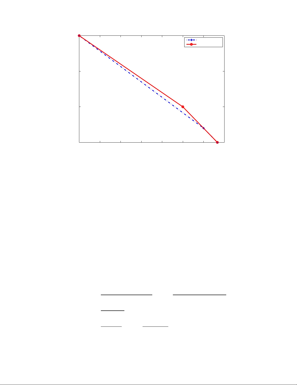
1 The Capacity Re gion of a Class of 3-Recei v er Broadcast Channels with De graded Message Sets Chandra Nair , Member , IEEE, and Abbas El Ga mal, F ellow , IEEE Abstract K ¨ orner and Marton established the c apacity region for the 2-receiver broadc ast chann el with d egraded message sets. Recent results and co njectures suggest that a straightforward extension of the K ¨ orner-Marton region to mo re than 2 receivers is optimal. This pap er shows th at th is is not the case. W e establish the capacity region f or a class of 3-recei ver broadc ast channels with 2 degraded message sets and show that it can b e strictly larger than the straightfor ward extension of the K ¨ o rner-Marton region . The key new idea is indirect decod ing, whereby a receiv er who cannot directly decode a cloud c enter , find s it indirectly by decoding satellite codew o rds. T his idea is then used to estab lish new in ner and outer b ounds on the capacity region of th e gen eral 3- receiver br oadcast channel with 2 an d 3 d egraded message sets. W e sh ow that these bo unds are tigh t for some nontrivial cases. Th e results suggest that the capacity of the 3-rec ei ver bro adcast chann el with d egraded message sets is as at least as hard to find as the capac ity o f the genera l 2-rece i ver br oadcast ch annel with common and private m essage. I . I N T RO D U C T I O N A broadcast channel with degraded message sets represents a scenario where a sender wishes to communicate a common message to all receiv ers, a first private m essage to a first subset of the receiv ers, a second priv ate message to a second sub set of the first subset and so o n. Such scenario can arise, for example, in video or m usic broadcasting over a wi reless network t o nested sub sets of recei vers at varying lev els of qualit y . The common message represents the lo west quality version to be sent to all receivers, the first p ri vate message represents the a ddi tional information needed for the fi rst subset of receivers to decode the second lowest quality version, and so on. W hat is the set of simultaneously achiev able ra t es for communicatin g su ch degrade d message sets over the network? This question was first studied by K ¨ orner and Marton in 1977 [1]. They considered a general 2-receiv er discrete-memoryless broadcast channel wit h sender X and recei vers Y 1 and Y 2 . A comm on message M 0 ∈ [1 , 2 nR 0 ] is to be sent to both receivers and a priv ate mess age M 1 ∈ [1 , 2 nR 1 ] is to be sent only to recei ver Y 1 . They showed that t he capacity region is given b y the set of all rate pairs ( R 0 , R 1 ) such that 1 R 0 ≤ min { I ( U ; Y 1 ) , I ( U ; Y 2 ) } , (1) R 1 ≤ I ( X ; Y 1 | U ) , for som e p ( u, x ) . These rates are achiev ed usi ng superposit ion coding [2]. The common message is represented by the auxi liary random variable U and the priv ate message is s uperimposed to generate X . The main contribution of [1] is proving a s trong con verse using the technique of images-of-a-set [3]. Extending the K ¨ orner -Marton result to more than 2 receiv ers has remained open ev en for the simpl e case of 3 recei vers Y 1 , Y 2 , Y 3 with 2 d egraded message sets, where a common message M 0 is to b e sent to all recei vers and a priv ate message M 1 is to be sent only to recei ver Y 1 . The s traightforward extension of t he K ¨ orner -Marton region to this case yields t he achiev able rate region consisti ng of t he set of all rate pairs ( R 0 , R 1 ) such that R 0 ≤ min { I ( U ; Y 1 ) , I ( U ; Y 2 ) , I ( U ; Y 3 ) } , (2) R 1 ≤ I ( X ; Y 1 | U ) , Chandra Nai r was partly supported by the Direct Grant for research at t he Chinese Unive rsit y of Hong K ong 1 The K ¨ orner-Ma rton characterization does not include the second term inside the min in the first inequality , I ( U ; Y 1 ) . Instead it includes the bound R 1 + R 2 ≤ I ( X ; Y 1 ) . It can be easily shown that the two characterizations are equi valent. 2 for some p ( u, x ) . Is this region optimal? In [4], it was shown that the above region (and i ts natural extension to k > 3 recei vers) is optim al for a class of product discrete-memoryless and Gaussian broadcast channels, wh ere each of the receive rs who decode only t he comm on message is a degraded version of the uni que receiv er that also decodes the priv ate m essage. In [5], it was shown that a straight forward extension of K ¨ orner -Marton region is optimal for the class of l inear determini stic broadcast channels, where t he operations are performed in a fi ni te fie ld . In addition to establ ishing the degraded message set capacity for t his cl ass the authors gav e an e xplicit characterization of the optimal auxil iary random v ariables. In a recent paper Borade et al. [6] introduced multilevel broadcast channels, w hich combine aspects of degraded broadcast channels and broadcast channels with degraded m essage sets. They established an achiev able rate region as well as a “mirror-image” outer bound for these channels. Their achiev able rate region is again a straightforward extension of the K ¨ orner -Marto n r egion to k -receiv er multilevel broadcast channels. I n particular , C onj ecture 5 of [6 ] states that t he capacity region for the 3 -recei ver m ultilevel broadcast channels d epicted i n Figure 1 is the set of all rate p airs ( R 0 , R 1 ) such that R 0 ≤ min { I ( U ; Y 2 ) , I ( U ; Y 3 ) } , (3) R 1 ≤ I ( X ; Y 1 | U ) , for s ome p ( u, x ) . Not e th at this region, henceforth referred to as the BZT r e gion , is the sam e as (2) because in the multi le vel broadcast channel Y 3 is a degraded version of Y 1 and therefore I ( U ; Y 3 ) ≤ I ( U ; Y 1 ) . P S f r a g r e p l a c e m e n t s X p ( y 1 , y 2 | x ) Y 1 p ( y 3 | y 1 ) Y 3 Y 2 Fig. 1. Multilev el 3-receiv er broadcast channels. Message M 0 is to be sent to all recei vers and message M 1 is to be sent only to Y 1 . In thi s paper we show that the st raightforward extension of the K ¨ orner -Marton r egion to more than 2 recei vers is not in general opt imal. W e establish the capacity region of the multilevel broadcast channels depicted in Figure 1 as the s et of rate pairs ( R 0 , R 1 ) such that R 0 ≤ min { I ( U 2 ; Y 2 ) , I ( U 1 ; Y 3 ) } , R 0 + R 1 ≤ min { I ( U 1 ; Y 3 ) + I ( X ; Y 1 | U 1 ) , I ( U 2 ; Y 2 ) + I ( X ; Y 1 | U 2 ) } , for some p ( u 1 ) p ( u 2 | u 1 ) p ( x | u 2 ) , and show that i t can be strictly larger than the BZT region. In our coding scheme, th e commo n message M 0 is represented by U 1 (the cloud centers), part of M 1 is s uperimposed on U 1 to ob tain U 2 (satellite code words), and the rest of M 1 is superimposed on U 2 to yi eld X . Recei vers Y 1 and Y 3 find M 0 by decoding U 1 , whereas receiv er Y 2 who may not be able to directly decode U 1 , finds M 0 indir ectly by decoding a list of satellite codew ords . After decoding U 1 , receiv er Y 1 finds M 1 by proceeding to decode U 2 then X . The rest of the paper is organized as follows. In Section II, we provide needed definitions. In Sec- tion III, we establish the capac it y region f or t he multileve l broadcast channel in F igu re 1 (Theorem 1). In Section IV, we show through an example that the capacity region for the mult ilev el broadcast channel can be strictly larger than t he BZT region. In Section V, we extend the results on the multi le vel b roadcast channel to establish inner and outer boun ds on the capacity region of the general 3-receiv er broadcast 3 channel wi th 2 degraded message sets (Propositio ns 5 and 6). W e show that these bounds are tight when Y 1 is less n oisy than Y 3 (Proposition 7), which is a m ore relaxed condi tion t han the degradedness conditi on of the mult ilev el broadcast channel m odel. W e then extend the inner bound t o 3 degraded message sets (Theorem 2). Alth ough Propositio n 5 is a special case of Theorem 2, it i s presented earlier for clarit y of exposition. Finally , we show that the inner bound of Theorem 2 when specialized to the case of 2 degraded message sets, where M 0 is t o be sent to all receiv ers and M 1 is to be s ent to Y 1 and Y 2 , reduces to the straight forward extension of the K ¨ orner -Marton region (Corollary 1). W e show that this inner bo und is tight for determini stic broadcast channels (Proposition 8) and when Y 1 is less noisy th an Y 3 and Y 2 is less noisy than Y 3 (Proposition 9). Finally , we outli ne a general approach to obtaining inner bounds on capacity for general k -receiver broadcast channel sce narios that us es the new idea of i ndirect decoding. I I . D E FI N I T I O N S Consider a discrete-memoryless 3-recei ver broadcast channel consisting of an input alphabet X , output alphabets Y 1 , Y 2 and Y 3 , and a probability transition functi on p ( y 1 , y 2 , y 3 | x ) . A (2 nR 0 , 2 nR 1 , n ) 2-de graded mess age set code for a 3-recei ver broadcast channel consists of (i) a pair of m essages ( M 0 , M 1 ) uniformly distrib ut ed ov er [1 , 2 nR 0 ] × [1 , 2 nR 1 ] , (ii) a n encoder that assig ns a code word x n ( m 0 , m 1 ) , for each message pair ( m 0 , m 1 ) ∈ [1 , 2 nR 0 ] × [1 , 2 nR 1 ] , and (iii) three decoders, one t hat maps each recei ved y n 1 sequence into an estimat e ( ˆ m 01 , ˆ m 1 ) ∈ [1 , 2 nR 0 ] × [1 , 2 nR 1 ] , a second that maps each recei ved y n 2 sequence in to an estimate ˆ m 02 ∈ [1 , 2 nR 0 ] , and a third that m aps each recei ved y n 3 sequence into an estim ate ˆ m 03 ∈ [1 , 2 nR 0 ] . The probability of error is defined as P ( n ) e = P { ˆ M 1 6 = M 1 or ˆ M 0 k 6 = M 0 for k = 1 , 2 , or 3 } . A rate tuple ( R 0 , R 1 ) is said to be achiev able if t here exists a sequence o f (2 nR 0 , 2 nR 1 , n ) 2-degraded message set codes with P ( n ) e → 0 . The capacity region of the broadcast channel i s the closure of the set of achiev able rates. A 3-receiv er m ultilevel broadcast channel [6] is a 3-receiver broadcast channel with 2 degraded message sets where p ( y 1 , y 2 , y 3 | x ) = p ( y 1 , y 2 | x ) p ( y 3 | y 1 ) for every ( x, y 1 , y 2 , y 3 ) ∈ X × Y 1 × Y 2 × Y 3 (see Figure 1). In additi on to considering the multilevel 3 -recei ver bro adcast channel and the general 3-recei ver b road- cast channel with 2 degraded message sets, we shall also con sider the following two scenarios: 1) 3-receiver broadcast channel with 3 m essage sets, where M 0 is to be sent to all recei vers, M 1 is to be sent to Y 1 and Y 2 , and M 2 is to be sent only to Y 1 . 2) 3-receiver broadcast channel with 2 degraded message sets, where M 0 is t o be s ent all receive rs and M 1 is to be sent to both Y 1 and Y 2 . Definitions of c odes, ac hi e vability and capacity regions for t hese cases are straightforwar d extensions of the abo ve definitions . Clearly , the 2 degraded message set scenarios are sp ecial cases of th e 3 degraded message set. Nev ertheless , we shall begin with the special class of multilev el broadcast channel because we are able to establ ish its capacity region. I I I. C A P A C I T Y O F 3 - R E C E I V E R M U LT I L E V E L B R OA D C A S T C H A N N E L The ke y resul t of this paper is given in the following theorem. Theor em 1: The capacity re gion of t he 3-recei ver multilevel broadcast channel in Figure 1 is the set of rate pairs ( R 1 , R 2 ) such that R 0 ≤ min { I ( U 1 ; Y 3 ) , I ( U 2 ; Y 2 ) } , (4) R 0 + R 1 ≤ min { I ( U 1 ; Y 3 ) + I ( X ; Y 1 | U 1 ) , I ( U 2 ; Y 2 ) + I ( X ; Y 1 | U 2 ) , } . for som e p ( u 1 ) p ( u 2 | u 1 ) p ( x | u 2 ) , where th e cardinalities of the auxiliary random variables satisfy kU 1 k ≤ kX k + 4 and k U 2 k ≤ kX k 2 + 5 kX k + 4 . 4 Remarks: 1) It is easy to show by sett ing U 1 = U 2 = U in the above theorem that the BZT region (3) is cont ained in t he capacity region (4). W e show in the next section that the capacity re gi on (4) can be strictly lar ger the BZT r egion. 2) It is straightforward to show that the a bove region is con vex and therefore there is no need t o use a time-sharing auxili ary random v ariable. The proof of Theorem 1 is given in the foll o wi ng s ubsections. A. Con verse W e s how that the region in Theorem 1 forms an outer bound to the capacity re gio n. The proof i s quite similar to previous weak con verse and outer bound p roofs for 2 -recei ver broadcast channels (e.g., see [7], [8], [9]). Supp ose we are given a sequence of codes for the multilevel broadcast channel with P ( n ) e → 0 . For each code, we form the empirical distribution for M 0 , M 1 , X n . Since X → Y 1 → Y 3 forms a physically de graded broadcast channel, it follows that the code rate pair ( R 0 , R 1 ) must satisfy the inequali ties R 0 ≤ I ( U 1 ; Y 3 ) , R 1 ≤ I ( X ; Y 1 | U 1 ) , for some p ( u 1 , x ) [7], where U 1 , X , Y 1 , Y 3 are defined as follows. Let U 1 i = ( M 0 , Y i − 1 1 ) , i = 1 , . . . , n , and let Q be a time-sharing random variable uniforml y distributed over the set { 1 , 2 , ..., n } and independent of X n , Y n 1 , Y n 2 , Y n 3 . W e then set U 1 = ( Q, U 1 Q ) and X = X Q , Y 1 = Y 1 Q , and Y 3 = Y 3 Q . Thus, we ha ve shown that R 0 ≤ I ( U 1 ; Y 3 ) , R 0 + R 1 ≤ I ( U 1 ; Y 3 ) + I ( X ; Y 1 | U 1 ) . Next, since t he decoding requirements of the broadcast channel X → ( Y 1 , Y 2 ) makes it a broadcast channel with degraded message sets, the code rate pair must sat isfy the inequalities R 0 ≤ min { I ( U 2 ; Y 2 ) , I ( U 2 , Y 1 ) } , R 0 + R 1 ≤ I ( U 2 ; Y 2 ) + I ( X ; Y 1 | U 2 ) , for some p ( u 2 , x ) [8], where U 2 is identified as follows. Let U 2 i = ( M 0 , Y i − 1 1 , Y n 2 i +1 ) , i = 1 , . . . , n , then we set U 2 = ( Q, U 2 Q ) . Combining the above tw o outer bounds, w e see t hat U 1 → U 2 → X forms a Mark ov chain. Ob serve that th is Markov nature of t he auxi liary random variables along wi th the degraded nature of X → Y 1 → Y 3 implies that I ( U 2 ; Y 1 ) ≥ I ( U 2 ; Y 3 ) ≥ I ( U 1 ; Y 3 ) . Thus we hav e shown that the code rate pair ( R 0 , R 1 ) must satisfy the inequali ties R 0 ≤ min { I ( U 1 ; Y 3 ) , I ( U 2 ; Y 2 ) } , R 0 + R 1 ≤ min { I ( U 1 ; Y 3 ) + I ( X ; Y 1 | U 1 ) , I ( U 2 ; Y 2 ) + I ( X ; Y 1 | U 2 ) } , for some p ( u 1 ) p ( u 2 | u 1 ) p ( x | u 2 ) . This establis hes the con verse to Theorem 1. B. Achie vabili ty The interesting p art of the proof of Theorem 1 i s achiev abili ty . Specifically , step 3 of the decoding procedure for Case 2 below describes a key contribution of this paper . W e show how Y 2 can find M 0 without directly decoding U n 1 or uniquely decoding U n 2 . 5 T o show achie vability of any rate pair ( R 0 , R 1 ) in region (4), because of its con ve xit y , it suffices to show the achiev abilit y of an y rate pair ( R 0 , R 1 ) such that R 0 = min { I ( U 1 ; Y 3 ) , I ( U 2 ; Y 2 ) } − δ R 0 + R 1 = min { I ( U 1 ; Y 3 ) + I ( X ; Y 1 | U 1 ) , I ( U 2 , Y 2 ) + I ( X ; Y 1 | U 2 ) } − 3 δ, for some U 1 → U 2 → X and any δ > 0 . Re writin g the second inequality we obtain R 0 + R 1 = I ( U 1 ; Y 3 ) + min { I ( U 2 ; Y 1 | U 1 ) , I ( U 2 ; Y 3 ) − I ( U 1 ; Y 3 ) } + I ( X ; Y 1 | U 2 ) − 3 δ . Now consider the fol lowing two cases: Case 1: I ( U 1 ; Y 3 ) > I ( U 2 ; Y 2 ) : The rates reduce to R 0 = I ( U 2 ; Y 2 ) − δ R 1 = I ( X ; Y 1 | U 2 ) − 2 δ . This pair can be achieved via a simple superposi tion coding scheme [2]. Case 2: I ( U 1 ; Y 3 ) ≤ I ( U 2 ; Y 2 ) : The rates reduce t o R 0 = I ( U 1 ; Y 3 ) − δ R 1 = I ( X ; Y 1 | U 2 ) + min { I ( U 2 ; Y 1 | U 1 ) , I ( U 2 , Y 2 ) − I ( U 1 ; Y 3 ) } − 2 δ. Let S 1 = min { I ( U 2 ; Y 1 | U 1 ) , I ( U 2 , Y 2 ) − I ( U 1 ; Y 3 ) } − δ and S 2 = I ( X ; Y 1 | U 2 ) − δ , then R 1 = S 1 + S 2 . Code Generation: Fix p ( u 1 ) p ( u 2 | u 1 ) p ( x | u 2 ) that satisfies the condi tion of Case 2. Generate 2 nR 0 = 2 n ( I ( U 1 ; Y 3 ) − δ ) sequences U n 1 (1) , . . . , U n 1 (2 nR 0 ) distributed uniformly at random over the set of ǫ -typical † U n 1 sequences, where δ → 0 as ǫ → 0 . For each U n 1 ( m 0 ) , generate 2 nS 1 = 2 n (min { I ( U 2 ; Y 1 | U 1 ) ,I ( U 2 ,Y 2 ) − I ( U 1 ; Y 3 ) }− δ ) sequences U n 2 ( m 0 , 1) , U n 2 ( m 0 , 2) , . . . , U n 2 ( m 0 , 2 nS 1 ) distrib ut ed uniformly at random ov er the set of condit ionally ǫ -typical U n 2 sequences. For each U n 2 ( m 0 , s 1 ) generate 2 nS 2 = 2 n ( I ( X ; Y 1 | U 2 ) − δ ) sequences X n ( m 0 , s 1 , 1) , X n ( m 0 , s 1 , 2) , . . . , X n ( m 0 , s 1 , 2 nS 2 ) distributed uniformly at random ove r the set of conditi onally ǫ -typical X n sequences. Encoding: T o send the m essage pai r ( m 0 , m 1 ) ∈ [1 , 2 nR 0 ] × [1 , 2 nR 1 ] , t he send er expresses m 1 by the pai r ( s 1 , s 2 ) ∈ [1 , 2 nS 1 ] × [1 , 2 nS 2 ] and sends X n ( m 0 , s 1 , s 2 ) . Decoding and Analysi s of Er r or Pr obability: 1) Receiv er Y 3 declares that m 0 is sent if it is the unique message such that U n 1 ( m 0 ) and Y n 3 are jointl y ǫ -typical. It i s easy t o s ee that this can be achieved with arbit rarily s mall prob ability of error because R 0 = I ( U 1 ; Y 3 ) − δ . 2) Receiv er Y 1 first declares that m 0 is sent if it is the un ique message such t hat U n 1 ( m 0 ) and Y n 1 are join tly ǫ -typical. Th is decodin g step succeeds with arbitrarily hi gh probabi lity because R 0 = I ( U 1 ; Y 3 ) − δ ≤ I ( U 1 ; Y 1 ) − δ . It t hen declares that s 1 is sent if i t is the unique index such that U n 2 ( m 0 , s 1 ) and Y n 1 are jointly ǫ -typical. This decoding step succeeds with arbitrarily high probability because S 1 ≤ I ( U 2 ; Y 1 | U 1 ) − δ . Finally it declares th at s 2 is sent if i t i s the unique i ndex such that X n ( m 0 , s 1 , s 2 ) and Y n 1 are joint ly ǫ -typical. This decoding step succeeds with high probabili ty because S 2 = I ( X ; Y 1 | U 2 ) − δ . 3) Receiv er Y 2 finds M 0 as follows. It declares t hat m 0 ∈ [1 , 2 nR 0 ] is sent if it is the un ique index such that U n 2 ( m 0 , s 1 ) and Y n 2 are jointly ǫ -typical for some s 1 ∈ [1 , 2 nS 1 ] . Suppose (1 , 1) ∈ [1 , 2 nR 0 ] × † W e assume strong typicality throughout this paper [10] . 6 [1 , 2 nS 1 ] is the message pair sent, then t he probabili ty of error avera ged over the choice of codebooks can be upper bound ed as follows P ( n ) e ≤ P { ( U n 2 (1 , 1) , Y n 2 ) are not joi ntly ǫ -typical } + P { ( U n 2 ( m 0 , s 1 ) , Y n 2 ) are joi ntly ǫ -typical for some m 0 6 = 1 } ( a ) < δ ′ + 2 n ( R 0 + S 1 ) X m 0 6 =1 X s 1 P { ( U n 2 ( m 0 , s 1 ) , Y n 2 ) jointly ǫ -typical } ( b ) ≤ δ ′ + 2 n ( R 0 + S 1 ) 2 − n ( I ( U 2 ; Y 2 ) − δ ) ( c ) ≤ δ ′ + 2 − nδ , where ( a ) follows by the uni on of events bound, ( b ) foll o ws by the fac t that for m 0 6 = 1 , U n 2 ( m 0 , s 1 ) and Y n 2 are generated completely in dependently and thus each probabilit y term under the sum is upper bounded by 2 − n ( I ( U 2 ; Y 2 ) − δ ) [10], ( c ) follows because by construction R 0 + S 1 ≤ I ( U 2 ; Y 2 ) − 2 δ , δ ′ → 0 as ǫ → 0 . Thus with a rbi trarily high prob ability , a ny jointly ǫ -typical U n 2 ( m 0 , s 1 ) with th e recei ved Y n 2 sequence must be of the form U n 2 (1 , s 1 ) , and receiver Y 2 can correctly decodes M 0 with arbit rarily small probability of error . Note that Y 2 may or may not be able t o uniquely decode U n 2 (1 , 1) . Ho wever , it finds t he correct common message wi th arbitrarily small probabil ity of error e ven if its rate R 0 > I ( U 1 ; Y 2 ) ! Thus all receivers can decode th eir intended messages with arbit rarily small probabi lity of error and hence t he rate p air R 0 = I ( U 1 ; Y 3 ) − δ, R 1 = I ( X ; Y 1 | U 2 ) + min { I ( U 2 ; Y 1 | U 1 ) , I ( U 2 , Y 2 ) − I ( U 1 ; Y 3 ) } − 2 δ is achie vable. This completes the proof of achiev abilit y of Theorem 1 . Remarks: 1) W e denote the decoding techniqu e used in step 3 as indire ct decoding , sin ce Y 2 decodes the cloud center U 1 indirectly by decoding satell ite code words. 2) There is no need t o break up the coding scheme into two cases. The coding scheme for Case 2 s uf fices. Thi s will become clear wh en we prove the achiev able region for the general case of 3-recei vers with 2 degraded message sets in Propositi on 5 . C. Bounds on Car di nality Using the strengthened Carath ´ eodory theorem by Fenchel and Eggleston [11] it can be readily s hown that for any choice of the auxiliary random va riable U 1 , there exists a random variable V 1 with cardinality bounded by kX k + 1 such that I ( U 1 ; Y 3 ) = I ( V 1 ; Y 3 ) and I ( X ; Y 1 | U 1 ) = I ( X ; Y 1 | V 1 ) . Similarly for any choice of U 2 , one can obtain a random variable V 2 with cardinality bou nded by kX k + 1 such th at I ( U 2 ; Y 2 ) = I ( V 2 ; Y 2 ) and I ( X ; Y 1 | U 2 ) = I ( X ; Y 1 | V 2 ) . Wh ile this preserves the re gion , it is not clear that the new random va riables V 1 , V 2 would preserve the Markov condition V 1 → V 2 → X . T o ci rcumvent this problem we adapt arguments from [11] to establ ish the cardinality bounds st ated in Theorem 1. For completeness, we provide an outline of the argument. Giv en U 1 → U 2 → X → ( Y 1 , Y 2 , Y 3 ) , we need to show t he e xis tence of random v ariables V 1 , V 2 such that the foll owing condi tions hold: V 1 → V 2 → X forms a Markov chain, I ( V 1 ; Y 3 ) = I ( U 1 ; Y 3 ) , I ( V 2 ; Y 2 ) = I ( U 2 ; Y 2 ) , I ( X ; Y 1 | V 1 ) = I ( X ; Y 1 | V 1 ) , and I ( X ; Y 1 | V 2 ) = I ( X ; Y 1 | U 2 ) . Further , the cardinalities of the new random variables must satisfy kV 1 k ≤ kX k + 4 , kV 2 k ≤ kX k 2 + 5 kX k + 4 . This argument is pro ved in two steps. In t he first step a random variable V 1 and transiti on probabil ities p ( u 2 | v 1 ) are constructed such that the following are held constant: p ( x ) , t he marginal probability of X (and hence Y 1 , Y 2 , Y 3 ), H ( Y 1 | U 1 ) , H ( Y 2 | U 1 ) , H ( Y 3 | U 1 ) , H ( Y 2 | U 2 , U 1 ) , and H ( Y 1 | U 2 , U 1 ) . Using standard ar gum ents [12], [11], t here exists a random v ariable V 1 and transition probabiliti es p ( u 2 | v 1 ) , with cardi- nality of V 1 bounded by k X k + 4 , such that the above equalities are achie ved. In particular the m ar ginal s 7 of X , Y 1 , Y 2 , Y 3 are held constant. Howe ver t he dis tribution of U 2 is not necessarily held const ant and hence we shall denote the resulti ng random v ariable as U ′ 2 . W e thu s ha ve random va riables V 1 → U ′ 2 → X such th at I ( V 1 ; Y 3 ) = I ( U 1 ; Y 3 ) , I ( V 1 ; Y 2 ) = I ( U 1 ; Y 2 ) , I ( X ; Y 1 | V 1 ) = I ( X ; Y 1 | U 1 ) , (5) I ( U ′ 2 ; Y 1 | V 1 ) = I ( U 2 ; Y 1 | U 1 ) . In the second step, for each V 1 = v 1 a new random v ariable V 2 ( v 1 ) is found such that the following are held constant: p ( x | v 1 ) , the marginal distribution of X conditioned on V 1 = v 1 , H ( Y 1 | U ′ 2 , V 1 = v 1 ) , and H ( Y 2 | U ′ 2 , V 1 = v 1 ) . Again standard ar guments imply that there exists a random variable V 2 ( v 1 ) and transition probabilities p ( x | v 2 ( v 1 )) , with cardinality of V 1 bounded by kX k + 1 , such that the above equalities are achiev ed. This in particular im plies that I ( V 2 ( V 1 ); Y 2 | V 1 ) = I ( U ′ 2 ; Y 2 | V 1 ) = I ( U 2 ; Y 2 | U 1 ) , (6) I ( V 2 ( V 1 ); Y 1 | V 1 ) = I ( U ′ 2 ; Y 1 | V 1 ) = I ( U 2 ; Y 1 | U 1 ) . Now , set V 2 = ( V 1 , V 2 ( V 1 )) and observe the following as a cons equence of Equations (5) and (6). I ( V 2 ; Y 2 ) = I ( V 1 ; Y 2 ) + I ( V 2 ( V 1 ); Y 2 | V 1 ) = I ( U 1 ; Y 2 ) + I ( U 2 ; Y 2 | U 1 ) = I ( U 2 ; Y 2 ) , I ( X ; Y 1 | V 2 ) = I ( X ; Y 1 | V 1 ) − I ( V 2 ( V 1 ); Y 1 | V 1 ) = I ( X ; Y 1 | U 1 ) − I ( U 2 ; Y 1 | U 1 ) = I ( X : Y 1 | U 2 ) . W e thus hav e the required random v ariables V 1 , V 2 satisfying t he cardinali ty bou nds kX k + 4 and ( kX k + 4)( kX k + 1) , respectively as desi red. I V . M U LT I L E V E L P R O D U C T B R OA D C A S T C H A N N E L In this section we show that the BZT region can be strictly smaller than the capacity re gion in Theorem 1. Consider the product of 3-receiv er broadcast channels gi ven by the M arko v relations hips X 1 → Y 21 → Y 11 → Y 31 , X 2 → Y 12 → Y 32 . (7) In Appendix I we derive the foll owing si mplified characterizations for the capacity and t he BZT regions. Pr opositio n 1: The BZT re gi on for th e above product channel reduces t o the set o f rate pairs ( R 0 , R 1 ) such that R 0 ≤ I ( V 1 ; Y 31 ) + I ( V 2 ; Y 32 ) , (8a) R 0 ≤ I ( V 1 ; Y 21 ) , (8b) R 1 ≤ I ( X 1 ; Y 11 | V 1 ) + I ( X 2 ; Y 12 | V 2 ) , (8c) for some p ( v 1 ) p ( v 2 ) p ( x 1 | v 1 ) p ( x 2 | v 2 ) . Pr opositio n 2: The capacity region for the product channel reduces to the set of rate p airs ( R 0 , R 1 ) such that R 0 ≤ I ( V 11 ; Y 31 ) + I ( V 12 ; Y 32 ) , (9a) R 0 ≤ I ( V 21 ; Y 21 ) , (9b) R 0 + R 1 ≤ I ( V 11 ; Y 31 ) + I ( V 12 ; Y 32 ) + I ( X 1 ; Y 11 | V 11 ) + I ( X 2 ; Y 12 | V 12 ) , (9c) R 0 + R 1 ≤ I ( V 21 ; Y 21 ) + I ( X 1 ; Y 11 | V 21 ) + I ( X 2 ; Y 12 | V 12 ) , (9d) for some p ( v 11 ) p ( v 21 | v 11 ) p ( x 1 | v 21 ) p ( v 12 ) p ( x 2 | v 12 ) . Now we comp are these two regions via the following example. 8 Example: Consider t he m ultileve l prod uct broadcast channel example in Figure 2, where: X 1 = X 2 = Y 12 = Y 21 = { 0 , 1 } , and Y 11 = Y 31 = Y 32 = { 0 , E , 1 } , Y 21 = X 1 , Y 12 = X 2 , t he channels Y 21 → Y 11 and Y 12 → Y 32 are binary erasure channels (BEC) with erasure probability 1 2 , and the channel Y 11 → Y 31 is give n by the transiti on probabil ities: P { Y 31 = E | Y 11 = E } = 1 , P { Y 31 = E | Y 11 = 0 } = P { Y 31 = E | Y 11 = 1 } = 2 / 3 , P( Y 31 = 0 | Y 11 = 0 } = P { Y 31 = 1 | Y 11 = 1 } = 1 / 3 . Therefore, the channel X 1 → Y 31 is ef fectively a BEC wit h erasure probability 5 / 6 . P S f r a g r e p l a c e m e n t s X 1 Y 21 Y 11 Y 31 X 2 Y 12 Y 32 1 / 2 1 / 2 2 / 3 2 / 3 1 / 2 1 / 2 1 / 2 1 / 2 1 / 3 1 / 3 1 / 2 1 / 2 0 1 0 1 0 E 1 0 E 1 Fig. 2. Product multilev el broadcast channel example. The BZT region can be simplified to the following. Pr opositio n 3: The BZT re gion for the above example reduces to the set of r ate pairs ( R 0 , R 1 ) satisfying R 0 ≤ min n p 6 + q 2 , p o , R 1 ≤ 1 − p 2 + 1 − q . (10) for some 0 ≤ p, q ≤ 1 . The p roof of t his proposition i s g iv en i n Appendix I. It is quite straightforward to see that ( R 0 , R 1 ) = ( 1 2 , 5 12 ) lies on the bound ary of this region. The capacity region can be simplified to the following Pr opositio n 4: The capacity region for the channel i n Figure 2 reduces t o set of rate pairs ( R 0 , R 1 ) satisfying R 0 ≤ min n r 6 + s 2 , t o , R 0 + R 1 ≤ min  r 6 + s 2 + 1 − r 2 + 1 − s, t + 1 − t 2 + 1 − s  , (11) for some 0 ≤ r ≤ t ≤ 1 , 0 ≤ s ≤ 1 . The proof of this propositio n is also given in Appendix I. Note t hat substituti ng r = t yields th e BZT region. By setting r = 0 , s = 1 , t = 1 it is easy to see that ( R 0 , R 1 ) = (1 / 2 , 1 / 2) lies on the boundary of the capacity region. On the other hand , for R 0 = 1 / 2 , the maxim um achie vable R 1 in the BZT region is 5 / 12 . Thus the capacity region is strictl y larger than the BZT region. 9 0 0.1 0.2 0.3 0.4 0.5 0.6 0.7 0 0.5 1 1.5 BZT region Capacity region (0.5, 0.5) (0.6, 0.2) (2/3, 0) P S f r a g r e p l a c e m e n t s R 1 R 0 Fig. 3. The B ZT and the capacity regions for t he channel i n Fi gure 2. Figure 3 p lots the BZT re gion and the capac it y region for the example channel. B ot h regions are specified by two line segments. The boundary of the BZT regions cons ists of the line se gm ents: (0 , 3 / 2) to (0 . 6 , 0 . 2) and (0 . 6 , 0 . 2) to (2 / 3 , 0) . The capacity region on t he other hand is formed by the pair of line segments: (0 , 3 / 2) to (1 / 2 , 1 / 2) and (1 / 2 , 1 / 2 ) to (2 / 3 , 0) . Note that t he boundaries of the tw o regions coincide on the li ne segment joini ng (0 . 6 , 0 . 2) to (2 / 3 , 0) . Remarks: 1) Consid er a 3-recei ver Gaussian product mult ilev el broadcast channel, where Y 21 = X 1 + Z 1 , Y 11 = Y 21 + Z 2 , Y 31 = Y 11 + Z 3 , Y 22 = X 2 + Z 4 , Y 32 = Y 22 + Z 5 . The noise power for Z i is N i for i = 1 , 2 , . . . , 5 . W e assume a total a verage p owe r constraint P on X = ( X 1 , X 2 ) . Using Gaussian signall ing it can be easily shown that t he BZT region is the set of all ( R 0 , R 1 ) such that R 0 ≤ C  αP 1 ¯ αP 1 + N 1 + N 2 + N 3  + C  β ( P − P 1 ) ¯ β ( P − P 1 ) + N 4 + N 5  , (12) R 0 ≤ C  αP 1 ¯ αP 1 + N 1  , R 1 ≤ C  ¯ αP 1 N 1 + N 2  + C  ¯ β ( P − P 1 ) N 4  , for some 0 ≤ P 1 ≤ P , 0 ≤ α, β ≤ 1 . Now if we us e Gaussian signali ng to ev aluate region (9), on e obtains the achie vable rate region 10 consisting of the set of all ( R 0 , R 1 ) such that R 0 ≤ C  a 1 P 1 ¯ a 1 P 1 + N 1 + N 2 + N 3  + C  a 2 ( P − P 1 ) ¯ a 2 ( P − P 1 ) + N 4 + N 5  , R 0 ≤ C  ( a 1 + b 1 ) P 1 (1 − a 1 − b 1 ) P 1 + N 1  , R 0 + R 1 ≤ C  ¯ a 1 P 1 N 1 + N 2  + C  ¯ a 2 ( P − P 1 ) N 4  + C  a 1 P 1 ¯ a 1 P 1 + N 1 + N 2 + N 3  + C  a 2 ( P − P 1 ) ¯ a 2 ( P − P 1 ) + N 4 + N 5  , (13) R 0 + R 1 ≤ C  ((1 − a 1 − b 1 ) P 1 N 1 + N 2  + C  (1 − a 2 − b 2 )( P − P 1 ) N 4  + C  ( a 1 + b 1 ) P 1 (1 − a 1 − b 1 ) P 1 + N 1  , for some 0 ≤ P 1 ≤ P , 0 ≤ a 1 , a 2 , b 1 , b 2 , a 1 + b 1 , a 2 + b 2 ≤ 1 . Now consider t he above regions wi th the parameters values: P = 1 , N 1 = 0 . 4 , N 2 = N 3 = 0 . 1 , N 4 = 0 . 5 , N 5 = 0 . 1 . Fixing R 1 = 0 . 5 log( 0 . 49 / 0 . 3) , we can sho w that the maximum achie vable R 0 in the Gaussian BZT region is 0 . 5 log (2 . 0566 ... ) . On the other hand, u sing the parameter values b 1 = 0 . 05 , 1 − a 1 = 0 . 1 725 , 1 − a 2 = 0 . 5079 , and P 1 = 0 . 5 680 for the region gi ven by (13), the pair (0 . 5 log( 2 . 0603) , 0 . 5 lo g(0 . 49 / 0 . 3)) i s in the exterior of the region. Thus restricted to Gaussian signalling the BZT r egion (8) is st rictly contained i n re gion (9). Ho wever , we have not been able to prove that Gaus sian signaling is optimal for either the BZT region or the capacity region. 2) The r eader may ask why we di d not consider the more general product channel X 1 → Y 21 → Y 11 → Y 31 , X 2 → Y 12 → Y 32 → Y 22 . In fact we consi dered this more general class at first but were unabl e to show that the capacity region conditions reduce to the separated form R 0 ≤ I ( V 11 ; Y 31 ) + I ( V 12 ; Y 32 ) , R 0 ≤ I ( V 21 ; Y 21 ) + I ( V 22 ; Y 22 ) , R 0 + R 1 ≤ I ( V 11 ; Y 31 ) + I ( V 12 ; Y 32 ) + I ( X 1 ; Y 11 | V 11 ) + I ( X 2 ; Y 12 | V 12 ) , R 0 + R 1 ≤ I ( V 21 ; Y 21 ) + I ( V 22 ; Y 22 ) + I ( X 1 ; Y 11 | V 21 ) + I ( X 2 ; Y 12 | V 12 ) , for some p ( v 11 ) p ( v 21 | v 11 ) p ( x 1 | v 21 ) p ( v 12 ) p ( v 22 | v 12 ) p ( x 2 | v 22 ) . V . B O U N D S O N C A PAC I T Y O F G E N E R A L 3 - R E C E I V E R B RO A D C A S T C H A N N E L W I T H D E G R A D E D M E S S A G E S E T S In this sectio n we extend the results in Section III t o obtain inn er and outer bou nds on the capacity region of general 3-receiv er broadcast channel wit h degraded message sets. W e first consider the same 2 degraded message set scenario as in Section III b ut without the condi tion that X → Y 1 → Y 3 form a degraded broadcast channel. W e est ablish inner and outer bounds for th is case and s how that they are tight when the channel X → Y 1 is less noisy than the c hannel X → Y 3 , which is a more general class than degraded broadcast channels [13]. W e t hen extend our results to the case o f 3 degraded mess age sets, where M 0 is t o be sent to all receiv ers, M 1 is t o be sent to receiver s Y 1 and Y 2 and M 2 is to be sent only to receiver Y 1 . A special case of this inner bound gives an inner bound to the capacity of the 2 degraded message set scenario where M 0 is to be sent to all receiv ers and M 1 is to be sent to recei vers Y 1 and Y 2 only . 11 A. Inner and Outer Bounds for 2 De graded Messag e S ets W e use superposition coding, indirect decoding, and the Marton achie vability scheme for the general 2-recei ver broadcast channels [14] to establ ish the following inner bo und. Pr opositio n 5: A ra te pair ( R 1 , R 2 ) is achiev able in a genera l 3-receive r broadcast channel with 2 degraded message sets if it satisfies the following i nequalities: R 0 ≤ min { I ( U 2 ; Y 2 ) , I ( U 3 ; Y 3 ) } , 2 R 0 ≤ I ( U 2 ; Y 2 ) + I ( U 3 ; Y 3 ) − I ( U 2 ; U 3 | U 1 ) , R 1 ≤ min { I ( X ; Y 1 | U 2 ) + I ( X ; Y 1 | U 3 ) , I ( X ; Y 1 | U 1 ) } , (14) R 0 + R 1 ≤ min { I ( X ; Y 1 ) , I ( U 2 ; Y 2 ) + I ( X ; Y 1 | U 2 ) , I ( U 3 ; Y 3 ) + I ( X ; Y 1 | U 3 ) } , 2 R 0 + R 1 ≤ I ( U 2 ; Y 2 ) + I ( U 3 ; Y 3 ) + I ( X ; Y 1 | U 2 , U 3 ) − I ( U 2 ; U 3 | U 1 ) , 2 R 0 + 2 R 1 ≤ I ( U 2 ; Y 2 ) + I ( X ; Y 1 | U 2 ) + I ( U 3 ; Y 3 ) + I ( X ; Y 1 | U 3 ) − I ( U 2 ; U 3 | U 1 ) , for some p ( u 1 , u 2 , u 3 , x ) = p ( u 1 ) p ( u 2 | u 1 ) p ( x, u 3 | u 2 ) = p ( u 1 ) p ( u 3 | u 1 ) p ( x, u 2 | u 3 ) (or i n other words, both U 1 → U 2 → ( U 3 , X ) and U 1 → U 3 → ( U 2 , X ) form Mark ov chains). Pr oof: The general idea of the proof is to represent M 0 by U 1 , superimpose two independent pieces of information about M 1 to obtain U 2 and U 3 , respectiv ely , and then superimp ose the remaining information about M 1 to obtain X . Recei ver Y 1 decodes U 1 , U 2 , U 3 , X , receiv ers Y 2 and Y 3 find M 0 via indirect decoding of U 2 and U 3 , respectiv ely , as in Theorem 1. W e now provide an out line of the proof Code Generation: Let R 1 = S 1 + S 2 + S 3 , where the S i ≥ 0 , i = 1 , 2 , 3 and T 2 ≥ S 2 , T 3 ≥ S 3 . Fix a probability mass function of the required form, p ( u 1 , u 2 , u 3 , x ) = p ( u 1 ) p ( u 2 | u 1 ) p ( x, u 3 | u 2 ) = p ( u 1 ) p ( u 3 | u 1 ) p ( x, u 2 | u 3 ) . Generate 2 nR 0 sequences U n 1 ( m 0 ) , m 0 ∈ [1 , 2 nR 0 ] distri b ut ed uniformly at random over the set of typi cal U n 1 sequences. For each U n 1 ( m 0 ) g enerate 2 nT 2 sequences U n 2 ( m 0 , t 2 ) , t 2 ∈ [1 , 2 nT 2 ] distributed uni formly at random from the set of conditionally typical U n 2 sequences, and 2 nT 3 sequences U n 3 ( m 0 , t 3 ) , t 3 ∈ [1 , 2 nT 3 ] distributed uniform ly at random over the set of conditionally typical U n 3 sequences. Randomly partition the 2 nT 2 sequences U n 2 ( m 0 , t 2 ) into 2 nS 2 equal size bin s and the 2 nT 3 U n 3 ( m 0 , t 3 ) s equences in to 2 nS 3 equal size bins . T o ensure that each product bin contains a jointly typical pair ( U n 2 ( m 0 , t 2 ) , U n 3 ( m 0 , t 3 )) with arbitrarily high probability , we r equi re that (see [15] for the proof) S 2 + S 3 < T 2 + T 3 − I ( U 2 ; U 3 | U 1 ) . (15) Finally for each chosen jointl y t ypical pair ( U n 2 ( m 0 , t 2 ) , U n 3 ( m 0 , t 3 )) in each produ ct bin ( s 2 , s 3 ) , generate 2 nS 1 sequences of codewords X n ( m 0 , s 2 , s 3 , s 1 ) , s 1 ∈ [1 , 2 nS 1 ] distributed uniformly at random over the set of conditionall y t ypical X n sequences. Encoding: T o send the m essage p air ( m 0 , m 1 ) , we express m 1 by the triple ( s 1 , s 2 , s 3 ) and send the code word X n ( m 0 , s 2 , s 3 , s 1 ) . Decoding: 1) Receiv er Y 1 declares that ( m 0 , s 2 , s 3 , s 1 ) i s s ent if it i s the unique rate tuple s uch th at Y n 1 is jointly typical wi th (( U n 1 ( m 0 ) , U n 2 ( m 0 , t 2 ) , U n 3 ( m 0 , t 3 ) , X n ( m 0 , s 2 , s 3 , s 1 )) , and s 2 is th e product bin nu mber of U n 2 ( m 0 , t 2 ) and s 3 is the product bin number of U n 2 ( m 0 , t 3 ) . Assuming ( m 0 , s 1 , s 2 , s 3 ) = (1 , 1 , 1 , 1) is sent, we partiti on the error ev ent into the following e vents. a) Error e vent corresponding to m 0 6 = 1 occurs with arbitrarily small probabilit y provided R 0 + S 1 + S 2 + S 3 < I ( X ; Y 1 ) . (16) b) Error event corresponding to m 0 = 1 , s 2 6 = 1 , s 3 6 = 1 occurs with arbitrarily small probability provided S 1 + S 2 + S 3 < I ( X ; Y 1 | U 1 ) . (17) 12 c) Error ev ent corresponding to m 0 = 1 , s 2 = 1 , s 3 6 = 1 occurs with arbitrarily small probability provided S 1 + S 3 < I ( X ; Y 1 | U 1 , U 2 ) = I ( X ; Y 1 | U 2 ) . (18) The equality follows from th e fact that U 1 → U 2 → ( U 3 , X ) form a Marko v Chain. d) Error event corresponding to m 0 = 1 , s 2 6 = 1 , s 3 = 1 occurs with arbitrarily small probability provided S 1 + S 2 < I ( X ; Y 1 | U 1 , U 3 ) = I ( X ; Y 1 | U 3 ) . (19) The above equality uses t he fa ct that U 1 → U 3 → ( U 2 , X ) form s a Markov chain. e) Error eve nt corresponding to m 0 = 1 , s 2 = 1 , s 3 = 1 , s 1 6 = 1 occurs w ith arbitrarily smal l probability provided S 1 < I ( X ; Y 1 | U 1 , U 2 , U 3 ) = I ( X ; Y 1 | U 2 , U 3 ) . (20) Note that the equality here u ses a weaker Markov structure U 1 → ( U 2 , U 3 ) → X . Thus recei ver Y 1 decodes ( m 0 , s 2 , s 3 , s 1 ) wi th arbitrarily small probability of error provided equations (16)-(20) hold. 2) Receiv er Y 2 decodes m 0 via list decoding of U n 2 ( m 0 , t 2 ) (as in Theorem 1). This can be achiev ed with arbitrarily sm all prob ability of error provided R 0 + T 2 < I ( U 2 ; Y 2 ) . (21) 3) Receiv er Y 3 decodes m 0 via list decoding of U n 2 ( m 0 , t 3 ) (as in Theorem 1). This can be achiev ed with arbitrarily sm all prob ability of error provided R 0 + T 3 < I ( U 3 ; Y 3 ) . (22) Combining equations (15)-(22) and using the F ourier-Motzkin procedure [16] to elimin ate T 2 , T 3 , S 1 , S 2 , and S 3 , we obtain the i nequalities in (14). The details are given in Appendi x II. Remarks: 1) The above ac hi e vability scheme can b e adapted to any jo int distribution p ( u 1 , u 2 , u 3 , x ) . Howe ver by l etting ˜ U 2 = ( U 2 , U 1 ) and letting ˜ U 3 = ( U 3 , U 1 ) we observe that th e region remains unchanged. Hence, w ithout los s of generality w e assume the structure of the auxiliary random v ariables as described in t he propo sition. It is also interesting t o n ote th at th e auxili ary random variables in the outer bound described i n the next subs ection also possess the same structure. 2) An interesting choice of the auxiliary random variables is to set U 2 or U 3 equal to U 1 (i.e., onl y one of the t he receiv ers tries to indirectly decode M 0 ), say let U 3 = U 1 . This reduces the inequalities 5 (after removing the redundant ones) to: R 0 ≤ min { I ( U 2 ; Y 2 ) , I ( U 1 ; Y 3 ) } , R 1 ≤ I ( X ; Y 1 | U 1 ) , (23) R 0 + R 1 ≤ min { I ( X ; Y 1 ) , I ( U 2 ; Y 2 ) + I ( X ; Y 1 | U 2 ) , I ( U 1 ; Y 3 ) + I ( X ; Y 1 | U 1 ) } , where U 1 → U 2 → X form a Markov chain. This region includes the capacity region of the m ultileve l case in Theorem 1. It is easy to verify that for any U 1 → U 2 → X that form a Markov chain, the corner poin ts of t he region in Theorem 1 satisfy the above i nequalities (and this suffices by conv exity). W e now establish the following outer bound 13 Pr opositio n 6: An y achiev able rate pair ( R 0 , R 1 ) for the gener al 3-recei ver broadcast channel with 2 degraded message sets must satisfy the conditions: R 0 ≤ min { I ( U 1 ; Y 1 ) , I ( U 2 ; Y 2 ) − I ( U 2 ; Y 1 | U 1 ) , I ( U 3 ; Y 3 ) − I ( U 3 ; Y 1 | U 1 ) } , R 1 ≤ I ( X ; Y 1 | U 1 ) . for some p ( u 1 , u 2 , u 3 , x ) = p ( u 1 ) p ( u 2 | u 1 ) p ( x, u 3 | u 2 ) = p ( u 1 ) p ( u 3 | u 1 ) p ( x, u 2 | u 3 ) , i.e., the same structure of the auxiliary random variables as in Lemma 5. F urth er one ca n restrict the car di nalities of U 1 , U 2 , U 3 to: kU 1 k ≤ kX k + 6 , kU 2 k ≤ ( kX k + 1)( k X k + 6) , and kU 3 k ≤ ( kX k + 1)( k X k + 6) . Pr oof: The proof follo ws lar gely standard arguments. T he auxiliary random variables are i dentified as U 1 i = ( M 0 , Y i − 1 1 ) , U 2 i = ( U 1 i , Y n 2 i +1 ) , U 3 i = ( U 1 i , Y n 3 i +1 ) . W ith this identification inequalities R 0 ≤ I ( U 1 ; Y 1 ) and R 1 ≤ I ( X ; Y 1 | U 1 ) is immediate. The other two i nequalities also follo w from st andard ar gum ents and is briefly outli ned here. nR 0 ≤ nλ n + X i I ( M 0 ; Y 3 i | Y n 3 i +1 ) ≤ nλ n + X i I ( M 0 , Y n 3 i +1 , Y i − 1 1 ; Y 3 i ) − I ( Y i − 1 1 ; Y 3 i | M 0 , Y n 3 i +1 ) ( a ) = nλ n + X i I ( M 0 , Y n 3 i +1 , Y i − 1 1 ; Y 3 i ) − I ( Y n 3 i +1 ; Y 1 i | M 0 , Y i − 1 1 ) = nλ n + X i I ( U 3 i ; Y 3 i ) − I ( U 3 i ; Y 1 i | U 1 i ) , where ( a ) uses the Csisz ´ ar sum equality . The cardinality bou nds are established usi ng a simil ar argument as in III-C. T o create a set of new auxiliary ra ndo m variables with the bounds o f Propos ition 6, we first replace U 2 by ( U 2 , U 1 ) and U 3 by ( U 3 , U 1 ) . It is easy to see from the Markov chain relationships U 1 → U 2 → ( U 3 , X ) and U 1 → U 3 → ( U 2 , X ) th at the following region is same as the that of Proposi tion 6. R 0 ≤ min { I ( U 1 ; Y 1 ) , I ( U 1 , U 2 ; Y 2 ) + I ( X ; Y 1 | U 1 , U 2 ) − I ( X : Y 1 | U 1 ) , I ( U 1 , U 3 ; Y 3 ) + I ( X ; Y 1 | U 1 , U 3 ) − I ( X : Y 1 | U 1 ) } , (24) R 1 ≤ I ( X ; Y 1 | U 1 ) . Then u sing standard ar gum ents one can replace U 1 by U ∗ 1 satisfying kU ∗ 1 k ≤ kX k + 6 , such that the distribution of X and H ( Y 1 | U 1 ) , H ( Y 1 | U 1 , U 2 ) , H ( Y 1 | U 1 , U 3 ) , H ( Y 2 | U 1 ) , H ( Y 2 | U 1 , U 2 ) , H ( Y 3 | U 1 ) , and H ( Y 3 | U 1 , U 3 ) are preserved. Now for each U ∗ 1 = u 1 one can find U ∗ 2 ( u 1 ) with cardinali ty less t han kX k + 1 each such that the distribution of X c on ditioned on U ∗ 1 = u 1 , H ( Y 1 | U ∗ 1 = u 1 , U 2 ) , and H ( Y 2 | U ∗ 1 = u 1 , U 2 ) are preserv ed. Similarly one can find for e ach U ∗ 1 = u 1 , a random variable U ∗ 3 ( u 1 ) with cardinali ty less than kX k + 1 each such that the dist ribution of X conditioned on U ∗ 1 = u 1 , H ( Y 1 | U ∗ 1 = u 1 , U 3 ) , and H ( Y 3 | U ∗ 1 = u 1 , U 3 ) are preserved. This yi elds random var iabl es U ∗ 1 , U ∗ 2 , U ∗ 3 that preserve the region in (24). (Note that as the distri b ut ion of X conditioned on U 1 = u 1 is preserved by both U ∗ 2 ( u 1 ) and U ∗ 3 ( u 1 ) , it is possible to get a consist ent tripl e of random variables U ∗ 1 , U ∗ 2 , U ∗ 3 .) Fin ally setti ng ˜ U 1 = U ∗ 1 , ˜ U 2 = ( U ∗ 1 , U ∗ 2 ) and ˜ U 3 = ( U ∗ 1 , U ∗ 3 ) gives the desired bou nds on cardinality as well as the desired Markov relations. Remarks: 1) The above outer bound appears to be very di f ferent from th e in ner bou nd of Propos ition 5 . Howev er , by taking app ropriate sums of the inequalities defining t he region of Proposition 6 , we arriv e at the 14 conditions R 0 ≤ min { I ( U 2 ; Y 2 ) − I ( U 2 ; Y 1 | U 1 ) , I ( U 3 ; Y 3 ) − I ( U 3 ; Y 1 | U 1 )) , R 1 ≤ I ( X ; Y 1 | U 1 ) , R 0 + R 1 ≤ min { I ( X ; Y 1 ) , I ( U 2 ; Y 2 ) + I ( X ; Y 1 | U 2 ) , I ( U 3 ; Y 3 ) + I ( X ; Y 1 | U 3 ) } , 2 R 0 + R 1 ≤ I ( U 2 ; Y 2 ) + I ( U 3 ; Y 3 ) + I ( X ; Y 1 | U 2 , U 3 ) − I ( U 2 ; U 3 | U 1 ) + I ( U 2 ; U 3 | Y 1 , U 1 ) . These con ditions incl ude s ome redundant ones, but are closer i n s tructure to the inequalit ies defining the inner boun d of Proposition 5. 2) The out er bound in Propositi on 6 reduces to t he capacity region for the m ultilevel case in Theorem 1. T o see thi s observe th at when X → Y 1 → Y 3 form a Markov chain, R 0 ≤ I ( U 3 ; Y 3 ) − I ( U 3 ; Y 1 | U 1 ) ≤ I ( U 3 ; Y 3 ) − I ( U 3 ; Y 3 | U 1 ) = I ( U 1 ; Y 3 ) . (25) Further from R 1 ≤ I ( X ; Y 1 | U 1 ) , we hav e R 0 + R 1 ≤ I ( U 1 ; Y 3 ) + I ( X ; Y 1 | U 1 ) . Thus the outer bound is contained in the achiev able region of Theorem 1, i.e., R 0 ≤ min { I ( U 1 ; Y 3 ) , I ( U 2 ; Y 2 ) } , (26) R 0 + R 1 ≤ { I ( U 1 ; Y 3 ) + I ( X ; Y 1 | U 1 ) , I ( U 2 ; Y 2 ) + I ( X ; Y 1 | U 2 ) } . 3) The inner and outer bounds match i f Y 1 is less noisy than Y 3 [13], that is if I ( U ; Y 3 ) ≤ I ( U ; Y 1 ) for a l l p ( u ) p ( x | u ) . As shown in [13], thi s condi tion is more general than degradedness. As such, it defines a larger class than multil e vel broadcast c hannel s. Pr opositio n 7: The c apacity region for the 3-recei ver broadcast channel wi th 2 de graded message sets when Y 1 is a less nois y recei ver than Y 3 is giv en by the set of rate p airs ( R 0 , R 1 ) such that R 0 ≤ min { I ( U 1 ; Y 3 ) , I ( U 2 ; Y 2 ) } , (27) R 0 + R 1 ≤ min { I ( U 1 ; Y 3 ) + I ( X ; Y 1 | U 1 ) , I ( U 2 ; Y 2 ) + I ( X ; Y 1 | U 2 ) } , for some p ( u 1 ) p ( u 2 | u 1 ) p ( x | u 2 ) . From the definition of less noi sy recei vers [13] we have I ( U 3 ; Y 3 | U 1 = u 1 ) ≤ I ( U 3 ; Y 1 | U 1 = u 1 ) for every choice of u 1 and thus I ( U 3 ; Y 3 | U 1 ) ≤ I ( U 3 ; Y 1 | U 1 ) for e very p ( u 1 ) p ( u 3 | u 1 ) p ( x | u 3 ) . Using (25) it follows that the general outer bound is contained in (27). The corner point of (27) (under the less noisy a ss umption) is contained in th e region g iv en by (23) and thus achiev able by setting U 3 = U 1 in the region of Proposition 5. B. Inner Bound for 3 De graded Messag e Sets In this section w e establish an i nner bound to the capacity region o f the broadcast channel with 3 degraded message sets where M 0 is to be sent to all three recei vers, M 1 is to be sent onl y to Y 1 and Y 2 , and M 2 is to be sent only to Y 1 . W e th en s pecialize t he result to the case of 2 degraded m essage sets s cenario, where M 0 is t o be sent to all receiver s and M 1 is to be sent to Y 1 and Y 2 and establi sh optimalit y for t wo class es of channels. The inner bound we establish is closely related to that of Proposition 5 . T o explain the connectio n, consider a 3-recei ver broadcast channel scenario where message M 0 is to be s ent to all t hree rece ivers, message M 12 is to be sent to recei vers Y 1 and Y 2 , message M 13 is to be sent to recei vers Y 1 and Y 3 , and message M 11 is to be s ent only to receiv er Y 1 . An inner boun d t o the capacity region for this scenario th at uses su perposition codi ng and Marton’ s coding scheme would be to represent M 0 by an auxil iary random var iabl e U 1 , ( M 0 , M 12 ) by an auxiliary random variable U 2 , ( M 0 , M 13 ) by U 3 , and ( M 0 , M 12 .M 13 , M 11 ) by X , where U 1 → U 2 → ( U 3 , X ) and U 1 → U 3 → ( U 2 , X ) form Marko v chains. The inner bound of P ropo sition 5 follows from the abo ve scenario by relaxing the conditions that Y 2 needs to decode M 12 and Y 3 needs to decode M 13 and considering both mess ages as parts of the 15 priv ate mess age t o receiv er Y 1 . Howe ver , instead of eliminati ng the auxiliary random variables U 2 and U 3 completely (as in the BZT region, which i s a straightforward extension of th e K ¨ orner -Marton scheme), we keep them and ha ve recei vers Y 2 and Y 3 use th e ne w technique of indirect decodi ng to find M 0 through U 2 and U 3 , respecti vely . As we ha ve sho wn in Section IV, ha ving these random variables U 2 and U 3 can strictly improve the achiev abilit y region of the 2-message sets s cenario. Now consider the 3 de graded message set scenario. W e relax the condition in t he above scenario that Y 3 needs t o decode M 13 . Recall the proof of Proposition 5. W e let R 1 = S 2 , R 2 = S 3 + S 1 and represent M 0 by U 1 , ( M 0 , M 1 ) by U 2 , ( M 0 , S 3 ) by U 3 , and ( M 0 , M 1 , M 2 ) by X . Recei ver Y 1 finds ( M 0 , M 1 , M 2 ) by decoding U 1 , U 2 , U 3 , X ; receiver Y 2 finds ( M 0 , M 1 ) by decoding U 1 , U 2 ; and receive r Y 3 finds M 0 by indirectly d ecoding U 1 through U 3 . W e obtain the foll owing conditions for achie vability of any rate tuple ( R 0 , R 1 , S 3 , S 1 ) by replacing S 2 by R 1 in condition s (15)-(22) and adding t he condition T 2 < I ( U 2 ; Y 2 | U 1 ) (to enable Y 2 to completely decode U 2 ). R 1 ≤ T 2 , S 3 ≤ T 3 , R 1 + S 3 ≤ T 2 + T 3 − I ( U 2 ; U 3 | U 1 ) , R 0 + S 1 + R 1 + S 3 ≤ I ( X ; Y 1 ) , S 1 + S 3 ≤ I ( X ; Y 1 | U 1 , U 2 ) = I ( X ; Y 1 | U 2 ) , S 1 + R 1 ≤ I ( X ; Y 1 | U 1 , U 3 ) = I ( X ; Y 1 | U 3 ) , (28) S 1 + R 1 + S 3 ≤ I ( X ; Y 1 | U 1 ) , S 1 ≤ I ( X ; Y 1 | U 1 , U 2 , U 3 ) = I ( X ; Y 1 | U 2 , U 3 ) , R 0 + T 2 ≤ I ( U 1 , U 2 ; Y 2 ) = I ( U 2 ; Y 2 ) , T 2 ≤ I ( U 2 ; Y 2 | U 1 ) , R 0 + T 3 ≤ I ( U 1 , U 3 ; Y 3 ) = I ( U 3 ; Y 3 ) , for some p ( u 1 , u 2 , u 3 , x ) = p ( u 1 ) p ( u 2 | u 1 ) p ( x, u 3 | u 2 ) = p ( u 1 ) p ( u 3 | u 1 ) p ( x, u 2 | u 3 ) . Performing Fourier -Motzkin procedure to eliminate the variables S 1 , S 3 , T 2 and T 3 yields the following achie vable region. Theor em 2: A rate triple ( R 0 , R 1 , R 2 ) is achiev able in a general 3-recei ver broadcast channel with 3 degraded message sets if it satisfies the condition s: R 0 ≤ I ( U 3 ; Y 3 ) R 1 ≤ min { I ( U 2 ; Y 2 | U 1 ) , I ( X ; Y 1 | U 3 ) } , R 2 ≤ I ( X ; Y 1 | U 2 ) R 0 + R 1 ≤ min { I ( U 2 ; Y 2 ) , I ( U 2 ; Y 2 | U 1 ) + I ( U 3 ; Y 3 ) − I ( U 2 ; U 3 | U 1 ) } , 2 R 0 + R 1 ≤ I ( U 2 ; Y 2 ) + I ( U 3 ; Y 3 ) − I ( U 2 ; U 3 | U 1 ) , R 0 + R 2 ≤ I ( U 3 ; Y 3 ) + I ( X ; Y 1 | U 2 , U 3 ) R 1 + R 2 ≤ I ( X ; Y 1 | U 1 ) , R 0 + R 1 + R 2 ≤ min { I ( X ; Y 1 ) , I ( U 3 ; Y 3 ) + I ( X ; Y 1 | U 3 ) , I ( U 2 ; Y 2 | U 1 ) + I ( U 3 ; Y 3 ) + I ( X ; Y 1 | U 2 , U 3 ) − I ( U 2 ; U 3 | U 1 ) } , (29) 2 R 0 + R 1 + R 2 ≤ I ( U 2 ; Y 2 ) + I ( U 3 ; Y 3 ) + I ( X ; Y 1 | U 2 , U 3 ) − I ( U 2 ; U 3 | U 1 ) , R 0 + 2 R 1 + R 2 ≤ I ( U 2 ; Y 2 | U 1 ) + I ( U 3 ; Y 3 ) + I ( X ; Y 1 | U 3 ) − I ( U 2 ; U 3 | U 1 ) , 2 R 0 + 2 R 1 + R 2 ≤ I ( U 2 ; Y 2 ) + I ( U 3 ; Y 3 ) + I ( X ; Y 1 | U 3 ) − I ( U 2 ; U 3 | U 1 ) . for some p ( u 1 , u 2 , u 3 , x ) = p ( u 1 ) p ( u 2 | u 1 ) p ( x, u 3 | u 2 ) = p ( u 1 ) p ( u 3 | u 1 ) p ( x, u 2 | u 3 ) (i.e., as before both U 1 → U 2 → ( U 3 , X ) and U 1 → U 3 → ( U 2 , X ) form Mark ov chains). 16 Remark: The region of Theorem 2 reduces to the inner boun d of Proposi tion 5 by setting R 1 = 0 . The equiv alence between the two descriptions is prove d in Appendi x III. W e no w consider a 2 degraded message set scenario where M 0 is to be sent to all recei vers and M 1 is to be sent to receive rs Y 1 and Y 2 . The fol lowing inner bound follows from Theorem 2 by setti ng R 2 = 0 . Cor ollary 1: A rate pair ( R 0 , R 1 ) is achie vable i n a 3-recei ver broadcast chann el with 2 de graded message sets, where M 0 is to be decoded by all three receiv ers and M 1 is to be decoded only b y Y 1 and Y 2 if it satisfies the following conditions: R 0 ≤ I ( U ; Y 3 ) , R 1 ≤ min { I ( X ; Y 2 | U ) , I ( X ; Y 1 | U ) } , (30) R 0 + R 1 ≤ min { I ( X ; Y 2 ) , I ( X ; Y 1 ) } , for some p ( u ) p ( x | u ) . Remarks: 1) Region (30) coincides wi th the straightforward e xtensi on of the K ¨ o rner -Marton 2-receiv er region. 2) By s etting R 2 = 0 , U 2 = X , and U 3 = U 1 = U the region in Theorem 2 reduces to (30). Thu s region in (30) is contained in region (29). 3) It may seem t hat the region obtained by setting R 2 = 0 i n (29) is lar ger than region (30), but they are in fact equal. variables, we see th at Therefore, there is no need to int roduce U 3 . T o prove this, observe that R 0 + R 1 ≤ I ( U 2 ; Y 2 | U 1 ) + I ( U 3 ; Y 3 ) − I ( U 2 ; U 3 | U 1 ) = I ( U 3 ; Y 3 ) + I ( U 3 ; Y 2 | U 1 ) + I ( U 2 ; Y 2 | U 3 ) − I ( U 3 ; Y 2 | U 2 ) − I ( U 3 ; U 2 | U 1 ) = I ( U 3 ; Y 3 ) + I ( U 2 ; Y 2 | U 3 ) − I ( U 3 ; U 2 | Y 2 , U 1 ) ≤ I ( U 3 ; Y 3 ) + I ( X ; Y 2 | U 3 ) . Thus the rate pairs m ust satisfy the following inequ alities R 0 ≤ I ( U 3 ; Y 3 ) , R 0 + R 1 ≤ min { I ( U 3 ; Y 3 ) + I ( X ; Y 2 | U 3 ) , I ( U 3 ; Y 3 ) + I ( X ; Y 1 | U 3 ) } , (31) R 0 + R 1 ≤ min { I ( X ; Y 2 ) , I ( X ; Y 1 ) } . Clearly this is contained ins ide region (30) and hence region ( 29 ) reduces to the one in Coroll ary 1 when R 2 = 0 . 4) Inner bo und (30) is opti mal for the following two special classes of broadcast channels. Pr opositio n 8: Achiev able region (30) is tight for deterministic 3-recei ver broadcast channels. It is straightforward to show that the set of rate pairs ( R 0 , R 1 ) such that R 0 ≤ min { H ( Y 1 ) , H ( Y 2 ) , H ( Y 3 ) } , R 0 + R 1 ≤ min { H ( Y 2 ) , H ( Y 1 ) } , for some p ( x ) const itutes an outer bound on t he capacity region. T o show a chieva bil ity , we need only consider the three choices for U : (i) U = Y 3 , and (ii) U = X , and (iii) U = ∅ . Pr opositio n 9: Achiev able region ( 30 ) is optimal when Y 1 is a less noisy recei ver than Y 3 and Y 2 is a less nois y recei ver than Y 3 . Note that t his result generalizes Theroem 3.2 in [4] where th e authors assume the receivers are Y 2 and Y 1 are de graded versions of Y 3 . T o show opti mality , we set U i = ( M 0 , Y i − 1 3 ) and thus the o nly 17 non-trivial inequality in th e conv erse is R 1 ≤ min { I ( X ; Y 1 | U ) , I ( X ; Y 2 | U ) } . T o see this observe that nR 1 ≤ X i I ( M 1 ; Y 1 i | M 0 , Y n 1 i +1 ) ≤ X i I ( M 1 ; Y 1 i | M 0 , Y n 1 i +1 , Y i − 1 3 ) + X i I ( Y i − 1 3 ; Y 1 i | M 0 , Y n 1 i +1 )) ( a ) = X i I ( M 1 , Y n 1 i +1 ; Y 1 i | M 0 , Y i − 1 3 ) − X i I ( Y n 1 i +1 ; Y 1 i | M 0 , Y i − 1 3 ) + X i I ( Y n 1 i +1 ; Y 3 i | M 0 , Y i − 1 3 ) ( b ) ≤ X i I ( X i ; Y 1 i | M 0 , Y i − 1 3 ) , where ( a ) uses the Csisz ´ ar sum equalit y and ( b ) uses the assumption that Y 1 is a less noisy than Y 3 , which impl ies that I ( Y n 1 i +1 ; Y 3 i | M 0 , Y i − 1 3 ) ≤ I ( Y n 1 i +1 ; Y 1 i | M 0 , Y i − 1 3 ) . The bound R 1 ≤ I ( X ; Y 2 | U ) can be proved si milarly . C. Inner Bounds for k -r eceiver Broadcast Channels The inner bounds dis cussed in previous subsections suggest the following extension to genera l k -receiv er broadcast channel scenarios with given message requirements . T o illust rate our procedure we shall use the runn ing example of a 3-receiv er broadcast channel wi th 3 messages to rec eiver subsets: { 1 } , { 1 , 2 } , and { 2 , 3 } . T o obtain an inner bound to capacity for a given message requirement, we first con sider all no nempty recei ver subsets. Let S D be th e collectio n of sub sets specified by the message requirements . For each A ∈ S D , we introduce an auxiliary random va riable for every B ⊃ A . Thus in our e xample, S D = {{ 1 } , { 2 , 3 } , { 1 , 2 }} , and five aux iliary random va riabl es are introduced corre spo nding to the s ubsets: { 1 , 2 , 3 } , { 1 , 2 } , { 1 , 3 } , { 2 , 3 } , and { 1 } . Let S I denote the re ceiver subsets for which auxiliary random var iabl es are introduced but are no t in S D . In the example, S I = {{ 1 , 3 } , { 1 , 2 , 3 }} . The receiv er s ubsets wi th auxili ary random v ariables assi gned to them are class ified in to levels based on their cardinality with the lowest le vel subsets ha ving th e lar gest cardinality . There i s a Mark ov structure between t he variables as follows: if U B represents t he auxil iary random variable corresponding to the subset B and U A represents the a ux iliary random v ariable correspondin g to the subset A ⊂ B , th en one can set U A = ( U B , ˜ U A ) . Thus an auxiliary random v ariable U A corresponding t o a subset A s hould cont ain all auxiliary random variables corresponding to the subsets B ⊃ A . For the running example, Le vel 1 contains the subset { 1 , 2 , 3 } , Level 2 con tains the subsets { 1 , 2 } , { 1 , 3 } , and { 2 , 3 } , and Level 3 contains the subset { 1 } . The M arko v relationships between these auxi liary random va riables are defi ned by: U 12 = ( U 123 , ˜ U 12 ) , U 13 = ( U 123 , ˜ U 13 ) , U 23 = ( U 123 , ˜ U 23 ) , U 1 = { U 12 , U 13 , ˜ U 1 } . Code generation proceeds one lev el at a ti me beginning with the lowest level followed by the second lowest le vel, and so on. The codebooks corresponding t o auxi liary random var iabl es at each lev el are randomly generated conditioned on codew ords at the lower level according to t he Markov structure of th e auxiliary random variables. Random binning is performed at each lev el to find jointl y ty pical code words to represent message products . Decoding is performed at recei ver i as follows: let T i represent the collection of recei ver subs ets that contains i for which auxili ary random variables are introduced. A subset A ∈ T i is said to be m inimal i f there is n o B ∈ T i such that B ⊂ A . Let T min i be the coll ection of mini mal subsets in T i . For the example 18 we obtain T 1 = {{ 1 , 2 , 3 } , { 1 , 2 } , { 1 , 3 } , { 1 }} and T min 1 = { 1 } , T 2 = {{ 1 , 2 , 3 } , { 1 , 2 } , { 2 , 3 }} and T min 2 = {{ 1 , 2 } , { 2 , 3 }} , T 3 = { 1 , 2 , 3 } , { 1 , 3 } , { 2 , 3 }} and T min 3 = {{ 1 , 3 } , { 2 , 3 } } . By the Markov structu re defined abov e, it is clear that all the messages for recei ver i are represented by the auxiliary random var i ables U min i , which correspond t o the elem ents of T min i . The auxi liary random var iabl es in U min i ∩ S D represent pri vate messages for recei ver i , while those in U min i ∩ S c D contain only parts of priv ate mess ages. Recei ver i uses indirect decoding to find the priv ate messages encoded into cloud centers by usin g th e satellite codew ords represented by the a uxi liary random va riables in U min i . In our running example, recei ver 3 indirectly decodes U 23 using the pair ( U 13 , U 23 ) . That is, the rate constraints are such that receiver 3 may not be able to uni quely decode U 13 but is abl e to decode the correct U 23 . Howe ver , receivers Y 2 and Y 1 should be able to correctly decode ( U 12 , U 23 ) and U 1 , respectively , and hence these receiv ers im pose the usual (direct) decoding const raints on the rates. In general, when U min i ∩ S I = ∅ , indirect decoding is not needed as in t he Examples below , where as in Proposition 5 indirect decoding is needed. The following two examples show that the above procedure yields the best known inner bounds for special classes of broadcast channels . Example 1: 2-recei ver broadcast channel where M 1 is to be decoded by receiv er Y 1 and M 2 is to be decoded by Y 2 . W e genera te 3 auxi liary random v ariables c orrespond ing to the three non-empty subsets of { 1 , 2 } : W for { 1 , 2 } , U for { 1 } and V for { 2 } . Setti ng ˜ U = ( U, W ) and ˜ V = ( V , W ) represents the M arko v structure among the variables. Observe that the auxiliary random v ariables are e xactly a s in Marton’ s coding scheme and so is the code generation we o utlined earlier . Example 2: k -recei ver broadcast channel with 2 degraded message sets, where M 0 is to be d ecoded by recei vers { 1 , . . . , k } a nd M 1 is to be decoded by { 1 , . . . , k − 1 } . The only sub sets that we would assign auxiliary random variables to here are { 1 , . . . , k } and { 1 , . . . , k − 1 } . W e thus introduce the auxili ary random var iabl e U 1 for { 1 , . . . , k } and U 2 for { 1 , . . . , k − 1 } . Th e re gio n is then be given by R 0 ≤ I ( U 1 ; Y k ) , R 0 + R 1 ≤ I ( U 2 ; Y i ) , for i = 1 , . . . , k − 1 , R 1 ≤ I ( U 2 ; Y i | U 1 ) for i = 1 , . . . , k − 1 , where U 1 → U 2 → X → { Y 1 , . . . , Y l } form a Markov chain. Clearly i n this case it is optim al t o set U 2 = X , which reduces the region to the straightforward extension of the K ¨ orner-Marton scheme. Remark: Our procedure can result in an explosion in the number of auxiliary random variables introduced e ven in simp le scenarios. Ho weve r , as we have shown in Section IV, indirect decoding may be needed to achie ve the capacity region for some classes of channels. Thus the introducti on of such a large number of auxiliary random variables m ay indeed be necessary in general. V I . C O N C L U S I O N Recent results and conjectures on the capacity of ( k > 2) -re ceiver broadcast channels with degra ded message sets [6], [4], [5] hav e lent support to the general belief that th e st raightforward extension of the K ¨ orner-Marton re gi on for t he 2-recei ver ca se is optim al. Thi s paper sho ws that this is not the case. W e show that the capacity region o f the 3-receiv er broadcast channels with 2 degraded message sets can be st rictly larger than the straightforward extension of the K ¨ orner -Marton re gi on. The achie vability proof uses the new idea of indirect decoding whereby a receiv er decodes a cloud center indi rectly throug h join t typicality w ith a satellit e codeword. Using this idea, we devise new inner bounds t o the capacity of the 19 general 3-recei ver broadcast channel with 2 and 3 degra ded message sets and show optimality in some cases. The structure of th e auxiliary random v ariables in the i nner bounds can be n aturally e xtended to more than 3 receivers. Th e bound s also provide so me insig ht into ho w the Marton achie vable rate region may be extended to more than 2 recei vers. The results in thi s paper sugg est that the capacity of the k > 2 -receiv er broadcast channels with degraded message sets is as at l east as h ard to find as t he capacity of th e general 2-recei ver broadcast channel wit h common and priv ate message. Howe ver , i t would be interesting to explore the opt imality of our new inner bounds for classes where capacity is known for the general 2-rec eiver case, such as deterministic and vector Gaussian broadcast channels. It would also be i nteresting to inv estigat e applications of indirect decoding to other problems, for example, 3 -recei ver broadcast channels with confidential message sets [11]. A C K N O L E D G E M E N T The authors wish t o thank Y oung-Han Kim for valuable sug gestions that has im prove d the presentatio n of this paper . R E F E R E N C E S [1] J. K ¨ orner and K. Marton, “General broadcast channels with deg raded message sets, ” IEE E T rans. Info. T heory , vol. IT -23, pp. 60–64, Jan, 1977. [2] T . Cov er, “Broadcast channels, ” IEEE Tr ans. Info. Theory , vol. I T -18, pp. 2–14, January , 1972. [3] J. K ¨ orner and K. Marton, “Images of a set via two channels and t heir role in mult-user communication, ” IEE E Tr ans. Info. Theory , vol. IT -23, pp. 751–76 1, Nov , 1977. [4] S. Diggavi and D. Tse, “On opportunistic codes and broadcast codes with degraded message sets, ” Information t heory workshop (ITW) , 2006. [5] V . Prabhakaran, S. Diggavi, and D. Tse, “Broadcasting with degraded message sets: A deterministic approach, ” P r oceedings of the 45th Annual Allerton Confer ence on Communication, Contro l and Computing , 2007. [6] S. Borade, L. Zheng, and M. Trott, “Multilev el broadcast networks, ” International Symposium on Information Theory , 2007. [7] R. G. Gallager , “Capacity and coding for degraded broadcast channels, ” Pr obl. P er edac. Inform. , vol. 10(3), pp. 3–14, 1974. [8] A. El Gamal, “The capacity of a class of broadcast channels, ” IEEE T rans. Info. Theory , vol. IT -25, pp. 166–169 , March, 1979. [9] C. Nair and A. E l Gamal, “ An outer bound to the capacity region of the broadcast channel, ” IEEE T rans. Info. T heory , vol. IT -53, pp. 350–35 5, January , 2007. [10] T . Cove r and J. Thomas, E lements of Information Theory . W iley Interscience, 1991. [11] I . Csiz ´ ar and J. K ¨ orner, “Broadcast channels with confidential messages, ” IE EE T rans. Info. Theory , vol. IT -24, pp. 339–348, May , 1978. [12] R . F . Ahlswede and J. K ¨ orner , “Source coding wi th side information and a con verse for degraded broadcast channels, ” IEEE T rans. Info. Theory , vol. IT -21(6), pp. 629–637, Novembe r, 1975. [13] J. K ¨ orner and K. Marton, “ A source network problem in volving the comparison of t wo channels ii, ” T rans. Colloquim Inform. Theory , K eszthely , Hungary , August, 1975. [14] K. Marton, “ A coding theorem for the discrete memoryless broadcast channel, ” IEE E T rans. Info. T heory , vol. IT -25, pp. 306–311, May , 1979. [15] A. El Gamal and E. C . van der Meulen, “ A proof of marton’ s coding theorem for the discrete memoryless broadcast channel, ” IEEE T ransaction s on Information Theory , vol. 27, no. 1, pp. 120–121, 1981. [16] A. Schrijver , Theory of Inte ger and Linear Pr ogramming . John Wile y & sons, 1986. 20 A P P E N D I X I P RO O F O F P RO P O S I T I O N S 1 , 2 , 3 , A N D 4 T o prove Propositions 1, 2, n ote t hat it is st raightforward to show that each si mplified characterization is contained in the ori ginal region as th e characterizations are obtai ned by us ing the channels independently . So we only prove t he other non-trivial direction. Pr oof of Pr opositi on 1: W e prov e that for the product broadcast channel g iv en by (7) the BZT region (3) reduces to the expression (8) . Consider the first term (8a) in th e BZT region R 0 ≤ I ( U ; Y 3 ) = I ( U ; Y 31 , Y 32 ) = I ( U ; Y 31 ) + I ( U ; Y 32 | Y 31 ) ≤ I ( U ; Y 31 ) + I ( U, Y 31 ; Y 32 ) ≤ I ( U ; Y 31 ) + I ( U, Y 11 ; Y 32 ) . Now set V 1 = U and V 2 = ( U, Y 11 ) . Thus the above inequ ality becomes R 0 ≤ I ( V 1 ; Y 31 ) + I ( V 2 ; Y 32 ) . The second term (8b) in th e BZT re gi on is simply given by R 0 ≤ I ( V 1 ; Y 21 ) . Finally , consider the last term (8c ) R 1 ≤ I ( X ; Y | U ) = I ( X 1 , X 2 ; Y 11 , Y 12 | U ) = H ( Y 11 , Y 12 | U ) − H ( Y 11 , Y 12 | X 1 , X 2 , U ) = H ( Y 11 | U ) + H ( Y 12 | U, Y 11 ) − H ( Y 11 | X 1 , U ) − H ( Y 12 | X 2 , U ) = I ( X 1 ; Y 11 | U ) + H ( Y 12 | U, Y 11 ) − H ( Y 12 | X 2 , U, Y 11 ) = I ( X 1 ; Y 11 | V 1 ) + I ( X 2 ; Y 12 | V 2 ) . The fact t hat p ( v 1 ) p ( v 2 ) p ( x 1 | v 1 ) p ( x 2 | v 2 ) suffices follows from the structu re of the mutual inform ation terms. Pr oof of Pr opositi on 2: W e prov e that for the product broadcast channel (7) the ca pacit y re gion gi ven by Theorem 1 reduces to the expression (9). Consider the first term (9a) in th e capacity region R 0 ≤ I ( U 1 ; Y 3 ) = I ( U 1 ; Y 31 , Y 32 ) = I ( U 1 ; Y 31 ) + I ( U 1 ; Y 32 | Y 31 ) ≤ I ( U 1 ; Y 31 ) + I ( U 1 , Y 31 ; Y 32 ) ≤ I ( U 1 ; Y 31 ) + I ( U 1 , Y 11 ; Y 32 ) . Now set V 11 = U 1 and V 12 = ( U 1 , Y 11 ) . The second term (9b) in the capacity region is R 0 ≤ I ( U 2 ; Y 21 ) . Now set V 21 = U 2 and from U 1 → U 2 → ( X 1 , X 2 ) we have V 11 → V 21 → X 1 . Thus the second term can be rewritten as R 0 ≤ I ( V 21 ; Y 21 ) 21 Consider the third term (9c) R 0 + R 1 ≤ I ( U 1 ; Y 3 ) + I ( X ; Y 1 | U 1 ) = I ( U 1 ; Y 31 , Y 32 ) + I ( X 1 , X 2 ; Y 11 , Y 12 | U 1 ) ≤ I ( U 1 ; Y 31 ) + I ( U 1 , Y 11 ; Y 32 ) + H ( Y 11 , Y 12 | U 1 ) − H ( Y 11 , Y 12 | X 1 , X 2 , U 1 ) = I ( U 1 ; Y 31 ) + I ( U 1 , Y 11 ; Y 32 ) + H ( Y 11 | U 1 ) + H ( Y 12 | U 1 , Y 11 ) − H ( Y 11 | X 1 , U 1 ) − H ( Y 12 | X 2 , U 1 , Y 11 ) = I ( V 11 ; Y 31 ) + I ( V 12 ; Y 32 ) + I ( X 1 ; Y 11 | V 11 ) + I ( X 2 ; Y 12 | V 12 ) . Finally consider the last term (9d) R 0 + R 1 ≤ I ( U 2 ; Y 21 ) + I ( X ; Y 1 | U 2 ) = I ( U 2 ; Y 21 ) + I ( X 1 , X 2 ; Y 11 , Y 12 | U 2 ) = I ( U 2 ; Y 21 ) + H ( Y 11 , Y 12 | U 2 ) − H ( Y 11 , Y 12 | X 1 , X 2 , U 2 ) ≤ I ( U 2 ; Y 21 ) + H ( Y 11 | U 2 ) + H ( Y 12 | U 2 , Y 11 ) − H ( Y 11 | X 1 , U 2 ) − H ( Y 12 | X 2 , U 2 , Y 11 ) = I ( V 21 ; Y 21 ) + I ( X 1 ; Y 11 | V 21 ) + I ( X 2 ; Y 12 | U 2 , Y 11 ) = I ( V 21 ; Y 21 ) + I ( X 1 ; Y 11 | V 21 ) + I ( X 2 ; Y 12 | U 2 , U 1 , Y 11 ) ≤ I ( V 21 ; Y 21 ) + I ( X 1 ; Y 11 | V 21 ) + I ( U 2 , X 2 ; Y 12 | U 1 , Y 11 ) = I ( V 21 ; Y 21 ) + I ( X 1 ; Y 11 | V 21 ) + I ( X 2 ; Y 12 | V 12 ) . The fact that p ( v 11 ) p ( v 21 ) p ( x 1 | v 21 ) p ( v 12 ) p ( x 2 | v 12 ) suffices fol lows from the structure of the mutu al i nfor - mation terms. In t he proof of propositi ons 3 and 4 we s hall make use of the following sim ple f act about the entropy function [10]. H ( ap, 1 − p, (1 − a ) p ) = H ( p, 1 − p ) + pH ( a, 1 − a ) . Pr oof of Pr opositi on 3: W e prove that the region giv en by (8) reduces to (10 ) for the binary erasure channel described by the example in Section IV. Let P { V 1 = i } = α i , P { X 1 = 0 | V 1 = i } = µ i . Then, I ( V 1 ; Y 31 ) = H X i α i µ i 6 , 5 6 , X i α i (1 − µ i ) 6 ! − X i α i H  µ i 6 , 5 6 , 1 − µ i 6  = 1 6 H X i α i µ i , X i α i (1 − µ i ) ! − 1 6 X i α i H ( µ i , 1 − µ i ) , I ( V 1 ; Y 21 ) = H X i α i µ i , X i α i (1 − µ i ) ! − X i α i H ( µ i , 1 − µ i ) , I ( X 1 ; Y 11 | V 1 ) = X i α i H  µ i 2 , 1 2 , 1 − µ i 2  − X i α i µ i H  1 2 , 1 2  − X i α i (1 − µ i ) H  1 2 , 1 2  = 1 2 X i α i H ( µ i , 1 − µ i ) . Similarly , let P { V 2 = i } = β i , P { X 2 = 0 | V 2 = i } = ν i . Then I ( V 2 ; Y 31 ) = 1 2 H X i β i ν i , X i β i (1 − ν i ) ! − 1 2 X i β i H ( ν i , 1 − ν i ) , I ( X 2 ; Y 12 | V 2 ) = X i β i H ( ν i , 1 − ν i ) . 22 Now setti ng P i β i H ( ν i , 1 − ν i ) = 1 − q , and P i α i H ( µ i , 1 − µ i ) = 1 − p , we o btain I ( U 1 ; Y 31 ) = 1 6 H X i α i µ i , X i α i (1 − µ i ) ! − 1 6 X i α i H ( µ i , 1 − µ i ) ≤ 1 6 (1 − (1 − p )) = p 6 , I ( U 1 ; Y 21 ) = H X i α i µ i , X i α i (1 − µ i ) ! − X i α i H ( µ i , 1 − µ i ) ≤ 1 − (1 − p ) = p, I ( X 1 ; Y 11 | U 1 ) = 1 − p 2 , I ( U 2 ; Y 31 ) = 1 6 H X i α i µ i , X i α i (1 − µ i ) ! − 1 6 X i α i H ( µ i , 1 − µ i ) ≤ 1 2 (1 − (1 − q )) = q 2 , I ( X 2 ; Y 12 | U 2 ) = 1 − q . Therefore, any rate pair in the BZT region must sati sfy the conditions R 0 ≤ min n p 6 + q 2 , p o , R 1 ≤ 1 − p 2 + 1 − q . for some 0 ≤ p, q ≤ 1 . It is easy to see that equality is achie ved when the marginals of V 1 are given by P { V 1 = 0 } = P { V 1 = 1 } = p/ 2 , P { V 1 = E } = 1 − p and t he marginals of V 2 are giv en b y P { V 2 = 0 } = P { V 2 = 1 } = q / 2 , P { V 2 = E } = 1 − q , (see Figu re 4). P S f r a g r e p l a c e m e n t s 1 / 2 1 / 2 V 1 X 1 0 E 1 0 1 0 E 1 0 1 1 / 2 1 / 2 V 2 X 2 p/ 2 1 − p p/ 2 q / 2 1 − q q / 2 Fig. 4. Auxiliary channels that achie ve the boundary of the BZT r egion . Pr oof of Pr opositi on 4: W e prove that the region (9) reduces to region (11) for th e bi nary erasure channel described by the example in Section IV. Assume that P { V 11 = i } = α i , P { X 1 = 0 | V 11 = i } = µ i , P { V 12 = i } = β i , P { X 2 = 0 | V 12 = i } = 23 ν i , P { V 21 = i } = γ i , P { X 1 = 0 | V 21 = i } = ω i . Further , there exist r , s, t ∈ [0 , 1] such that H ( X 1 | V 11 ) = X i α i H ( µ i , 1 − µ i ) = 1 − r , H ( X 2 | V 12 ) = X i β i H ( ν i , 1 − ν i ) = 1 − s, H ( X 1 | V 21 ) = X i γ i H ( ω i , 1 − ω i ) = 1 − t. Clearly from the Markov condition V 11 → V 21 → X 1 , we require 1 − t ≤ 1 − r or equi valently r ≤ t . W e can also establ ish the following in a similar fashion. I ( V 11 ; Y 31 ) = 1 6 H X i α i µ i , X i α i (1 − µ i ) ! − 1 6 X i α i H ( µ i , 1 − µ i ) ≤ r 6 , I ( V 12 ; Y 32 ) = 1 2 H X i β i ν i , X i β i (1 − ν i ) ! − 1 2 X i β i H ( ν i , 1 − ν i ) ≤ s 2 , I ( V 21 ; Y 21 ) = H X i γ i ω i , X i γ i (1 − ω i ) ! − X i γ i H ( ω i , 1 − ω i ) ≤ t, I ( X 1 ; Y 11 | V 11 ) = 1 2 X i α i H ( µ i , 1 − µ i ) = 1 − r 2 , I ( X 2 ; Y 12 | V 12 ) = X i β i H ( ν i , 1 − ν i ) = 1 − s, I ( X 1 ; Y 11 | V 21 ) = 1 2 X i γ i H ( ω i , 1 − ω i ) = 1 − t 2 . Thus any rate pair in the capacity region must satisfy R 0 ≤ min n r 6 + s 2 , t o , R 0 + R 1 ≤ min  r 6 + s 2 + 1 − r 2 + 1 − s, t + 1 − t 2 + 1 − s  , for some 0 ≤ r ≤ t ≤ 1 , 0 ≤ s ≤ 1 . Note that sub stituting r = t yields t he BZT region. Equality in the above cond itions is achiev ed by the choices of auxiliary random variables shown in Figure 5, and thus the above region is th e capacity region. P S f r a g r e p l a c e m e n t s 1 / 2 1 / 2 V 11 X 1 0 E 1 0 1 0 E 1 0 1 1 / 2 1 / 2 V 12 X 2 r/ 2 ¯ r r/ 2 s/ 2 ¯ s s/ 2 ( t − r ) / 2 ( t − r ) / 2 V 21 Fig. 5. Auxiliary channels that achie ve the boundary of the capacity region . 24 A P P E N D I X I I F O U R I E R - M O T Z K I N E L I M I NA T I O N F O R P RO P O S I T I O N 5 In this section we provide the details of the Fourier -Mot zkin procedure in the proof of Proposition 5. T o elimi nate T 2 , T 3 we need to consider the following set of inequalities S 2 ≤ T 2 , S 3 ≤ T 3 , S 2 + S 3 ≤ T 2 + T 3 − I ( U 2 ; U 3 | U 1 ) , R 0 + T 2 ≤ I ( U 2 ; Y 2 ) , R 0 + T 3 ≤ I ( U 2 ; Y 3 ) . Eliminati on T 2 first we end up with S 3 ≤ T 3 , R 0 + S 2 + S 3 ≤ I ( U 2 ; Y 2 ) + T 3 − I ( U 2 ; U 3 | U 1 ) , R 0 + S 2 ≤ I ( U 2 ; Y 2 ) , R 0 + T 3 ≤ I ( U 2 ; Y 3 ) . Eliminati on of T 3 in the above leads us to 2 R 0 + S 2 + S 3 ≤ I ( U 2 ; Y 2 ) + I ( U 2 ; Y 3 ) − I ( U 2 ; U 3 | U 1 ) , R 0 + S 2 ≤ I ( U 2 ; Y 2 ) , R 0 + S 3 ≤ I ( U 2 ; Y 3 ) . Thus any pair R 0 , R 1 = S 1 + S 2 + S 3 that satisfies the following s et of inequalities is achiev able S 1 ≥ 0 , S 2 ≥ 0 , S 3 ≥ 0 , R 0 + S 2 ≤ I ( U 2 ; Y 2 ) , R 0 + S 3 ≤ I ( U 3 ; Y 3 ) , 2 R 0 + S 2 + S 3 ≤ I ( U 2 ; Y 2 ) + I ( U 3 ; Y 3 ) − I ( U 2 ; U 3 | U 1 ) , R 0 + S 2 + S 3 + S 1 ≤ I ( X ; Y 1 ) , S 2 + S 3 + S 1 ≤ I ( X ; Y 1 | U 1 ) , S 2 + S 1 ≤ I ( X ; Y 1 | U 3 ) , S 3 + S 1 ≤ I ( X ; Y 1 | U 2 ) , S 1 ≤ I ( X ; Y 1 | U 2 , U 3 ) . 25 Substitutin g for S 1 = R 1 − S 2 − S 3 yields S 2 ≥ 0 , S 3 ≥ 0 , S 2 + S 3 ≤ R 1 , R 0 + S 2 ≤ I ( U 2 ; Y 2 ) , R 0 + S 3 ≤ I ( U 3 ; Y 3 ) , 2 R 0 + S 2 + S 3 ≤ I ( U 2 ; Y 2 ) + I ( U 3 ; Y 3 ) − I ( U 2 ; U 3 | U 1 ) , R 0 + R 1 ≤ I ( X ; Y 1 ) , R 1 ≤ I ( X ; Y 1 | U 1 ) , R 1 ≤ S 3 + I ( X ; Y 1 | U 3 ) , R 1 ≤ S 2 + I ( X ; Y 1 | U 2 ) , R 1 ≤ S 2 + S 3 + I ( X ; Y 1 | U 2 , U 3 ) . Eliminati on of S 2 leads to 0 ≤ S 3 R 0 + S 3 ≤ I ( U 3 ; Y 3 ) , R 0 + R 1 ≤ I ( X ; Y 1 ) , R 1 ≤ I ( X ; Y 1 | U 1 ) , R 1 ≤ S 3 + I ( X ; Y 1 | U 3 ) , S 3 ≤ R 1 , R 0 ≤ I ( U 2 ; Y 2 ) , 2 R 0 + S 3 ≤ I ( U 2 ; Y 2 ) + I ( U 3 ; Y 3 ) − I ( U 2 ; U 3 | U 1 ) , S 3 ≤ I ( X ; Y 1 | U 2 ) , R 0 + R 1 ≤ I ( U 2 ; Y 2 ) + I ( X ; Y 1 | U 2 ) , 2 R 0 + R 1 + S 3 ≤ I ( U 2 ; Y 2 ) + I ( U 3 ; Y 3 ) − I ( U 2 ; U 3 | U 1 ) + I ( X ; Y 1 | U 2 ) , 0 ≤ I ( X ; Y 1 | U 2 , U 3 ) redundant, R 0 + R 1 ≤ I ( U 2 ; Y 2 ) + S 3 + I ( X ; Y 1 | U 2 , U 3 ) , 2 R 0 + R 1 ≤ I ( U 2 ; Y 2 ) + I ( U 3 ; Y 3 ) + I ( X ; Y 1 | U 2 , U 3 ) − I ( U 2 ; U 3 | U 1 ) . Finally eliminating S 3 (and removing redundant inequalities) leads one to the region in Propositio n 5. A P P E N D I X I I I P RO O F O F R E M A R K 1 F O L L O W I N G T H E O R E M 2 Consider the 3-recei ver broadcast channel with 3 degraded m essage sets. Let R 2 = S 1 + S 2 + S 3 . The proof is in three steps: 26 ( i ) First, we show th at any rate tuple ( R 0 , R 1 , S 1 , S 2 , S 3 ) is achiev able provided R 1 ≤ T 21 , S 2 ≤ T 22 , S 3 ≤ T 3 , R 1 + S 3 ≤ T 21 + T 3 − I ( ˜ U 2 ; U 3 | U 1 ) , R 1 + S 2 + S 3 ≤ T 21 + T 22 + T 3 − I ( U 2 ; U 3 | U 1 ) , R 0 + S 1 + R 1 + S 2 + S 3 ≤ I ( X ; Y 1 ) , S 1 + R 1 + S 2 + S 3 ≤ I ( X ; Y 1 | U 1 ) , S 1 + S 2 + S 3 ≤ I ( X ; Y 1 | ˜ U 2 ) , (32 ) S 1 + S 3 ≤ I ( X ; Y 1 | U 2 ) , S 1 + R 1 + S 2 ≤ I ( X ; Y 1 | U 3 ) , S 1 + S 2 ≤ I ( X ; Y 1 | U 3 , ˜ U 2 ) , S 1 ≤ I ( X ; Y 1 | U 2 , U 3 ) , R 0 + T 21 + T 22 ≤ I ( U 2 ; Y 2 ) , T 21 ≤ I ( ˜ U 2 ; Y 2 | U 1 ) , R 0 + T 3 ≤ I ( U 3 ; Y 3 ) , for p ( u 1 , ˜ u 2 , u 2 , u 3 , x ) = p ( u 1 ) p ( ˜ u 2 | u 1 ) p ( u 2 | ˜ u 2 ) p ( x, u 3 | u 2 ) = p ( u 1 ) p ( u 3 | u 1 ) p ( ˜ u 2 , u 2 | u 3 ) p ( x | u 2 , u 3 ) , i.e. U 1 → U 3 → ( ˜ U 2 , U 2 , X ) and U 1 → ˜ U 2 → U 2 → ( U 3 , X ) form Marko v chains. ( ii ) Then, we show that the region d efined by (32) is equal to th e inner bound in Theorem 2. ( iii ) Finally we show that wh en R 1 = 0 , t he c ond itions (32) reduce to conditions ( 15)-(22) in t he proof of Proposition 5, thus completin g the proof of Remark 1. A. Achie vabili ty of Rat es Satisfying (32) First we outline the achiev ability o f any rate tuple ( R 0 , R 1 , S 1 , S 2 , S 3 ) t hat satisfies conditions (32). Code generation is ve ry similar to that in the proof of Proposit ion 5. W e insert ˜ U 2 , an aux iliary random var iabl e representing the information about M 1 , between U 1 and U 2 ; so for every U n 1 ( m 0 ) we generate 2 nT 21 U n 2 ( m 0 , m 1 ) sequences and randoml y partition them into 2 nR 1 bins. For each ˜ U n 2 ( m 0 , m 1 ) , we generate 2 nT 22 U n 2 ( m 0 , m 1 , t 21 ) sequences and randomly partition them into 2 nS 2 bins. W e t hen generate 2 nT 3 U n 3 ( m 0 , t 3 ) sequences and partition them into 2 nS 3 bins. For each p roduct bin (( m 1 , s 2 ) , s 3 ) we select a jointly typical pair ( U n 2 ( m 0 , m 1 , t 2 ) , U n 3 ( m 0 , t 3 )) . Finally for product bin (( m 1 , s 2 ) , s 3 ) with corresponding jointly typical ( U n 2 ( m 0 , m 1 , t 2 ) , U n 3 ( m 0 , t 3 )) pair , we generate 2 nS 1 sequences X n ( m 0 , m 1 , s 2 , s 3 , s 1 ) . T o ensure correct code generation (existence of relev ant jointly typical sequences) we require t hat R 1 ≤ T 21 , S 2 ≤ T 22 , S 3 ≤ T 3 , R 1 + S 3 ≤ T 21 + T 3 − I ( ˜ U 2 ; U 3 | U 1 ) , R 1 + S 2 + S 3 < T 21 + T 22 + T 3 − I ( U 2 ; U 3 | U 1 ) . 27 Recei ver Y 1 uses joint typi cality to find ( m 0 , m 1 , s 1 , s 2 , s 3 ) . The following condit ions on the probabil ity of error ensure successful decodi ng (the corresponding e vents that partition the error event are li sted). R 0 + S 1 + R 1 + S 2 + S 3 < I ( X ; Y 1 ) , ( e vent: ˆ m 0 6 = 1) S 1 + R 1 + S 2 + S 3 < I ( X ; Y 1 | U 1 ) , ( e vent: ( ˆ m 0 = 1 , ˆ m 1 6 = 1 , ˆ s 3 6 = 1)) S 1 + S 2 + S 3 < I ( X ; Y 1 | ˜ U 2 ) , ( e vent: ( ˆ m 0 = 1 , ˆ m 1 = 1 , ˆ s 2 6 = (1 , 1) , ˆ s 3 6 = 1)) S 1 + S 3 < I ( X ; Y 1 | U 2 ) , ( e vent: ( ˆ m 0 = 1 , ˆ m 1 = 1 , ˆ s 2 = (1 , 1) , ˆ s 3 6 = 1)) S 1 + R 1 + S 2 < I ( X ; Y 1 | U 3 ) , ( e vent: ( ˆ m 0 = 1 , ˆ s 3 = 1 , ˆ m 1 6 = 1)) S 1 + S 2 < I ( X ; Y 1 | U 3 , ˜ U 2 ) , ( e vent: ( ˆ m 0 = 1 , ˆ s 3 = 1 , ˆ m 1 = 1 , ˆ s 2 6 = (1 , 1))) S 1 < I ( X ; Y 1 | U 2 , U 3 ) , ( e vent: ( ˆ m 0 = 1 , ˆ s 3 = 1 , ˆ m 1 = 1 , ˆ s 2 = (1 , 1) , ˆ s 1 6 = 1)) . Recei ver Y 2 decodes m 0 via indirect decoding using U 2 and m 1 by decoding ˜ U 2 conditioned on U 1 . Th is is successful provided R 0 + T 21 + T 22 < I ( U 2 ; Y 2 ) , T 21 < I ( ˜ U 2 ; Y 2 | U 1 ) . Recei ver Y 3 decodes m 0 via indirect decoding using U 3 . This step succeeds provided R 0 + T 3 < I ( U 3 ; Y 3 ) . Combining the above condi tions we see that any rate tuple satisfying (32) is achiev able. B. Equivalence of Conditions (32) to Theor em 2 In one direction, s etting ˜ U 2 = U 2 , S 2 = 0 , T 22 = 0 and T 21 = T 2 , we obtain (28). Thus conditions (32) contain the region described by Theorem 2. For the r everse direction we b reak down the argument into two cases. Case 1: T 22 < I ( U 2 ; Y 2 | ˜ U 2 ) Observe that Y 2 can also decode S 2 and settin g ˜ R 1 = R 1 + S 2 , ˜ R 2 = R 2 − S 2 , and T 21 + T 22 = T 2 we see that conditi ons (32) along wi th T 22 < I ( U 2 ; Y 2 | ˜ U 2 ) im ply conditions (28). Thus under T 22 < I ( U 2 ; Y 2 | ˜ U 2 ) , the region described by (32) is contained in the region described by Theorem 2. Case 2: T 22 < I ( U 2 ; Y 2 | ˜ U 2 ) If T 22 ≥ I ( U 2 ; Y 2 | ˜ U 2 ) , then the condition R 0 + T 21 + T 22 < I ( U 2 ; Y 2 ) impl ies that R 0 + T 21 < I ( ˜ U 2 ; Y 2 ) and Y 2 ’ s requirement for successful decoding can be changed to R 0 + T 21 < I ( ˜ U 2 ; Y 2 ) , T 21 < I ( ˜ U 2 ; Y 2 | U 1 ) . In the rest of the inequali ties, replacing U 2 by ˜ U 2 only weakens th em and h ence it is o ptimal to set U 2 = ˜ U 2 . These new in equalities imply (28) in w hich we replace S 1 by S 1 + S 2 and U 2 by ˜ U 2 . Thus under T 22 > I ( U 2 ; Y 2 | ˜ U 2 ) also, the region describ ed by (32) is contai ned in the region described by Theorem 2. Combining Cases 1 and 2 we see that rate pairs satisfying con ditions (32) is contained in t he re gio n described by Theorem 2. This compl etes the proof of their equiv alence. 28 C. Reduction to Pr o position 5 If R 1 = 0 , the region described b y conditions (32) reduce to 0 ≤ T 21 , S 2 ≤ T 22 , S 3 ≤ T 3 , S 3 ≤ T 21 + T 3 − I ( ˜ U 2 ; U 3 | U 1 ) , S 2 + S 3 ≤ T 21 + T 22 + T 3 − I ( U 2 ; U 3 | U 1 ) , S 1 + S 2 + S 3 ≤ I ( X ; Y 1 | ˜ U 2 ) , R 0 + S 1 + S 2 + S 3 ≤ I ( X ; Y 1 ) , S 1 + S 2 + S 3 ≤ I ( X ; Y 1 | U 1 ) , (33) S 1 + S 3 ≤ I ( X ; Y 1 | U 2 ) , S 1 + S 2 ≤ I ( X ; Y 1 | U 3 ) , S 1 + S 2 ≤ I ( X ; Y 1 | U 3 , ˜ U 2 ) S 1 ≤ I ( X ; Y 1 | U 2 , U 3 ) R 0 + T 21 + T 22 ≤ I ( U 2 ; Y 2 ) , T 21 ≤ I ( ˜ U 2 ; Y 2 | U 1 ) R 0 + T 3 ≤ I ( U 3 ; Y 3 ) . Recalling that R 2 = S 2 + S 3 + S 1 , and setti ng ˜ T 22 = T 21 + T 22 , observe t hat any ( R 0 , S 1 , S 2 , S 3 ) satis fying the above inequaliti es (33) also satisfies S 2 ≤ ˜ T 22 , S 3 ≤ T 3 , S 2 + S 3 ≤ ˜ T 22 + T 3 − I ( U 2 ; U 3 | U 1 ) , R 0 + S 1 + S 2 + S 3 ≤ I ( X ; Y 1 ) , S 1 + S 2 + S 3 ≤ I ( X ; Y 1 | ˜ U 2 ) , S 1 + S 3 ≤ I ( X ; Y 1 | U 2 ) , S 1 + S 2 ≤ I ( X ; Y 1 | U 3 ) , S 1 + S 2 ≤ I ( X ; Y 1 | U 3 , ˜ U 2 ) , S 1 ≤ I ( X ; Y 1 | U 2 , U 3 ) , R 0 + ˜ T 22 ≤ I ( U 2 ; Y 2 ) , R 0 + T 3 ≤ I ( U 3 ; Y 3 ) . These conditi ons are clearly m aximized by set ting ˜ U 2 = U 1 which in turn reduces t he equations to conditions (15)-(22) of 5.. Th us the region defined by (33) is con tained in the region giv en by Proposi tion 5. The other direction is direct as the region i n Proposition 5 is obtained by setting ˜ U 2 = U 1 in (33). This completes the proof of Remark 1. Remark: Observe that we do not need the auxil iary random variable ˜ U 2 to characterize the region in either the 3 degraded message sets case (Theorem 2) or the 2 degraded m essage sets case (Proposition 5). This is in accordance with the structure of auxili ary random v ariables as prescribed by the remark in the introduction of Subsection V -B.