The price of certainty: "waterslide curves" and the gap to capacity

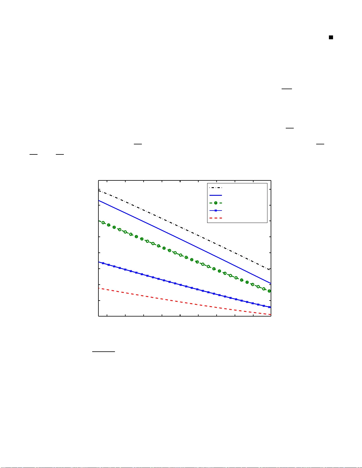
The price of cert ainty: “wat erslide curv es” and the gap to capa city Anant Sahai and Pulkit Gro ver W ireless F oundations, Department of EE CS Univ ersity of California at Berkele y , CA-9472 0, USA { sahai, pul kit } @eecs.berkeley .edu Abstract The classical problem of reliable point-to-p oint digital commun ication is to achieve a low pro bability o f error while keep ing the rate h igh an d the tota l power consumption small. T rad itional inform ation-the oretic analysis uses e xplicit models fo r the com munication channel to study the p ower spent in transmission. Th e resulting bou nds are expressed u sing ‘waterfall’ cur ves that co n vey the revolutionary idea that un bound edly low pro babilities of bit- error ar e attainab le using o nly ﬁnite transmit power . Howe ver , practition ers have long observed that th e decoder complexity , and hence the total power consump tion, go es up when a ttempting to use sophisticated cod es that operate close to the waterfall curve. This p aper gives a n explicit mod el fo r p ower consumptio n at an idealized deco der tha t allows for extreme parallelism in implemen tation. The decod er ar chitecture is in th e spirit o f message passing an d iterative decod ing for sparse-gr aph codes, b ut is fur ther idealized in that it allows for more comp utational po wer than is currently known to be im plementable . Gen eralized sphere-p acking argu ments a re used to derive lower boun ds o n the d ecoding power needed for any possible code given only the gap fro m the Shanno n limit an d the desired pr obability of e rror . As the g ap goes to zero, th e en er gy p er bit spent in decod ing is shown to go to inﬁnity . This sug gests th at to op timize total power , the transmitter sho uld opera te at a power that is strictly above th e minimu m dem anded by the Sh annon capacity . The lo wer bound is plotted to sho w an una voidable tradeoff between the a verage bit-error probability and the total power u sed in transmission an d d ecoding . I n the spirit of conventional waterfall cu rves, we call these ‘waterslide’ curves. Th e boun d is shown to be ord er optimal b y showing the existence of code s th at can ach iev e similarly shaped waterslide curves unde r th e prop osed idealized model of decodin g. 1 The price of cert ainty: “wat erslide curv es” and the gap to capa city Note: A preli minary version of this work with weaker bounds was submitted to ITW 2 008 in P orto [1] . I . I N T RO D U C T I O N As digital circuit techno logy advances a nd we p ass into the era of billion-transistor ch ips, it is clear that the fundamental limit o n practical c odes is n ot any nebulous sen se o f “c omplexity” but the co ncrete iss ue of p ower consump tion. At the same time, the proposed ap plications for error-correcting codes continue to shrink in the distances in volved. Whe reas earlier “deep space communication” helped stimulate the development o f information and co ding theory [2], [3], there is now an increas ing interest in communica tion over much shorter d istances ranging from a few meters [4] to even a few millimeters in the ca se of inter-chip and on-ch ip communication [5]. The implications of power -consumption beyond transmit power have b egun to be studied b y the co mmunity . Th e common threa d in [6]–[10] is that the power consu med in proc essing the signals can be a sub stantial fraction of the total power . In [11], it is o bserved that within communication n etworks, it is worth developing cross-layer sc hemes to reduc e the time that devices spen d being a cti ve. In [9], an information-theoretic formulation is c onsidered . When the transmitter is in the ‘on’ state, its circuit is modeled as consuming s ome ﬁxed po wer in addition to the power radiated in the trans mission itself. The refore, it ma kes sens e to sh orten the overall duration of a packet transmission and to satisfy an average transmit-po wer constraint by b ursty signalling that does not u se all av ailable degrees of freed om. In [7], the a uthors take into accou nt a pea k-power con straint as well, as they stud y the optimal constellation size for uncode d transmission. A lar ge c onstellation requires a smaller ‘on’ time, and hence les s circuit power . Howe ver , a lar ger con stellation requires highe r power to ma intain the same s pacing of cons tellation points. An optimal cons tellation has to balanc e b etween the tw o, but overall this argues for the us e of high er rates. Howe ver , none of these really tac kle the role of the decod ing complexity itself. In [12], the authors take a more rece i ver -centric view and focu s o n how to limi t the power spen t in sampling the signal at the receiv er . T hey point ou t that empirically for ultrawideband sy stems aiming for moderate probabilities of e rror , this sa mpling cost can be lar ger than the de coding cost! They introduce the ingenious idea of ada pti vely puncturing the c ode at the rece i ver rathe r than a t the transmitter . Th ey implicitly ar gue for the us e o f long er codes whose rates are further from the Shannon capac ity so that the decod er ha s the ﬂexibili ty to adaptively pun cture as needed an d thereby save on total p ower c onsumption. In [4], the a uthors study the impact of dec oding complexity us ing the metric of co ding gain. They take an empirical point of view using power -co nsumption numbers for certain decoder implementations a t moderately lo w probabilities of error . They o bserve that it is o ften better to us e n o coding at all if the communication ran ge is lo w enough . In this p aper , we take an as ymptotic approach to see if cons idering decoding power has any fundamen tal implications as the av erage probability of bit error tends to zero. In Section II, we gi ve a n asymptotic formulation of what it should mean to app roach c apacity when we mus t conside r the p ower spen t in decoding in add ition to that spent in transmission. W e next c onsider whether c lassical approa ches to enco ding/decod ing su ch as de nse linear block codes and con v olutional co des ca n sa tisfy our stricter standa rd of approa ching ca pacity and argue that they cannot. Se ction III then focuses our a ttention on iterativ e de coding by message pa ssing and de ﬁnes the system model for the rest o f the paper . Section IV de ri ves g eneral lower bounds to the c omplexity of iterative de coders for BSC a nd A WGN c hanne ls in terms of the numb er of iterations required to achieve a des ired probab ility of error at a given transmit power . These bounds can be cons idered iterative-decoding co unterparts to the classical sphere-pac king bound s (see e.g. [13], [14]) and are deri ved by gene ralizing the d elay-oriented ar guments of [15], [16] to the decoding neighborhoods in iterati ve decod ing. T hese boun ds are then used to show that it is in principle poss ible for iterativ e dec oders to b e a part of a weak ly ca pacity-achieving communication system. Howe ver , the power s pent by our mod el of an iterati ve decode r must go to inﬁn ity as the probability of e rror tends to zero and so this s tyle of de coding rules out a strong sense of capac ity-achieving c ommunication systems . 2 W e discu ss related work in the sparse -graph-code context in Sec tion V and make prec ise the notion of gap to capac ity before evaluating our lower -bounds on the n umber of iterations as the g ap to capa city c loses. W e c onclude in Sec tion VI with some spec ulation and point o ut some interes ting ques tions for future in vestigation. I I . C E RT A I N T Y - AC H I E V I N G C O D E S Consider a classica l po int-to-point A WGN cha nnel with no fading. For uncode d transmiss ion with BPSK sig- naling, the probability of b it-error is an exponentially d ecreasing function o f the trans mitted ene r gy per symb ol. T o approac h certainty (make the probability of bit-error very small), the transmitted energy pe r symbo l must go to inﬁnity . If the sy mbols e ach carry a s mall n umber of bits, the n this implies that the transmit power is also g oing to inﬁnity sinc e the number of symb ols pe r second is a nonzero constant determined by the desired rate of R bits per se cond. Shannon ’ s gen ius in [17] was to recog nize that while there was no way to av oid having the transmitted ene r gy go to inﬁn ity and s till approach certainty , this ene r gy could be a mortized over ma ny b its of information. This mean t that the transmitted power cou ld be kept ﬁnite and certainty c ould be approa ched by paying for it using end-to-end delay (see [16] for a revie w) and whatever implemen tation complexity is required for the enc oding and decod ing. For a giv en cha nnel an d transmit power P T , there is a maximum rate C ( P T ) that ca n b e supported. T urned arou nd, this classical res ult is tr aditionally expressed by ﬁxing the d esired rate R a nd looking a t the required transmit power . The res ulting “ waterf all curves” a re shown 1 in F igure 1. These sha rp curves are distinguished from the more grad ual “waterslide curves” of unco ded transmission. 0 0.5 1 1.5 2 2.5 3 3.5 −6 −5.5 −5 −4.5 −4 −3.5 −3 −2.5 −2 −1.5 −1 Power log 10 ( 〈 P e 〉 ) Uncoded transmission BSC Shannon Waterfall BSC Shannon Waterfall AWGN Fig. 1. The S hannon waterfalls: plots of log ( h P e i ) vs required SNR (in dB) for a ﬁxed rate- 1 / 3 code transmitted using BPSK o ver an A WGN channel wit h hard decisions at t he detector . A comparison is made with t he rate- 1 / 3 repetition code: uncoded tr ansmission with the same bit repeated t hree times. Also sho wn is the waterfall curve for the average po wer constrained A WGN channel. T raditionally , a family of c odes was cons idered c apacity a chieving if it c ould su pport arbitrarily low p robabilities of e rror at transmit powers arbitrarily c lose to that predicted by capacity . T he c omplexity of the en coding an d decoding steps was con sidered to be a sep arate and qua litati vely distinct performance metric. T his makes s ense 1 Since the focus of this paper is on average bit error probab ility , these curves combine the results of [17], [18] and adjust the required capacity by a factor of the relev ant rate-distortion function 1 − h b ( h P e i ) . 3 when the communica tion is long-range, since the “exchan ge rate” b etween transmitter power and the power that ends up being de li vered to the rece i ver is very poor due to distan ce-induced attenuation. In light of the adva nces in digital cir cuits a nd the n eed for sh orter-range communication, we pr opose a new way of formalizing what it means for a coding app r oach to be “capacity achieving” using the single natural metric: power . A. Deﬁ nitions Assume the traditional information-theoretic mo del (se e e. g. [13], [19]) of ﬁxed-rate disc rete-time co mmunication with k total information bits, m c hanne l uses , and the rate of R = k m bits per channe l us e. As is traditional, the rate R is held c onstant wh ile k and m are allowed to beco me asy mptotically large. h P e,i i is the av erage p robability of bit error on the i -th mess age bit and h P e i = 1 k P i h P e,i i is used to deno te the overall a verage p robability of bit error . No restrictions are ass umed on the c odebook s aside from those required by the chann el mode l. The channel model is assume d to be indexed by the power used in transmission. The encode r and de coder are a ssumed to b e physical entities tha t cons ume po wer according to some mod el that ca n be different for different codes . Let ξ T P T be the ac tual power us ed in transmission and let P C and P D be the power co nsumed in the operation of the encod er and decod er respectiv ely . ξ T is the exchang e rate (total path-loss ) that c onnects the power spen t at the transmitter to the rec eiv ed power P T that shows up at the receiver . In the sp irit of [10], we a ssume that the goal o f the sy stem de signer is to minimize some w eighted combination P total = ξ T P T + ξ C P C + ξ D P D where the vector ~ ξ > 0 . The we ights ca n be dif ferent de pending o n the application 2 and ξ T is tied to the distance be tween the transmitter a nd receiver as well a s the propa gation en vironment. For any rate R and average p robability of bit error h P e i > 0 , we ass ume t hat the system designer wil l minimize the weighted combination above to get o ptimized P total ( ~ ξ , h P e i , R ) as well as constituent P T ( ~ ξ , h P e i , R ) , P C ( ~ ξ , h P e i , R ) , and P D ( ~ ξ , h P e i , R ) . Deﬁnition 1: The certainty of a particular encod ing and deco ding sy stem is the reciprocal of the a verage probability of bit error . Deﬁnition 2: An enco ding and dec oding sys tem at rate R bits per se cond is we akly certainty achieving if lim inf h P e i→ 0 P T ( ~ ξ , h P e i , R ) < ∞ for all weigh ts ~ ξ > 0 . If an e ncoder/dec oder system is not wea kly c ertainty a chieving, then this me ans that it doe s no t d eli ver on the rev olutionary promise of the Shann on waterf all cu rve from the perspec ti ve o f trans mit power . Instead , such c odes encourag e s ystem des igners to pay for certainty using unboun ded transmission power . Deﬁnition 3: An encoding and decoding s ystem at rate R bits per second is str ongly certainty achie ving if lim inf h P e i→ 0 P total ( ~ ξ , h P e i , R ) 6 = ∞ for a ll weights ~ ξ > 0 . A strongly certainty-achieving system would de li ver on the full s pirit of S hannon ’ s vision: that certainty ca n be approached at ﬁnite total po wer just by accepting longe r end-to-end de lays a nd a mortizing the total energy expenditure over ma ny bits. The general d istinction be tween strong and we ak ce rtainty-achieving systems relates to how the decoding power P D ( ~ ξ , h P e i , R ) varies with the p robability of bit-error h P e i for a ﬁxed rate R . Does it have waterf all or waterslide behavior? For example, it is clea r tha t uncoded transmission has very s imple encoding /decoding 3 and so P D ( ~ ξ , h P e i , R ) has a waterfall behavior . Deﬁnition 4: A { weakly | strongly } ce rtainty-achieving system a t rate R bits p er second is als o { weak ly | str ongly } capacity achieving if lim inf ξ C ,ξ D → ~ 0 lim inf h P e i→ 0 P T ( ~ ξ , h P e i , R ) = C − 1 ( R ) (1) where C − 1 ( R ) is the minimum transmiss ion power tha t is pred icted by the Shannon c apacity of the channe l mo del. 2 For example, in an RF ID application, the po wer used by the t ag i s actually supplied wirelessly by the reader . If the tag is the decoder , then it is natural to make ξ D e ven larger than ξ T in order to account for the inefﬁcienc y of the power transfer from the reader to the tag. One-to-many transmission of multi cast data is another example of an application that can increase ξ D . T he ξ D in that case should be increased in proportion to the number of receiv ers that are listening to the message. 3 All that is required is the minimum po wer needed t o sample the receiv ed signal and threshold the result. 4 This sens e of capa city achieving makes explicit the sense in which we should conside r encoding a nd d ecoding to be asy mptotically fr ee , but no t actua lly free. T he traditional approa ch of mo deling e ncoding an d dec oding as being actua lly free can be recovered by swapping the orde r of the limits in (1). Deﬁnition 5: An e ncoding and dec oding system is c onsidered traditionally capac ity achieving if lim inf h P e i→ 0 lim inf ξ C ,ξ D → ~ 0 P T ( ~ ξ , h P e i , R ) = C − 1 ( R ) . (2) where C − 1 ( R ) is the minimum transmiss ion power tha t is pred icted by the Shannon c apacity of the channe l mo del. By taking the limit ( ξ C , ξ D ) → 0 for a ﬁxed probability of error , this traditional ap proach makes it imposs ible to cap ture any fundamental tradeoff with complexity in an a symptotic sen se. The conce ptual distinction betwee n the new (1 ) and old (2) sense s o f c apacity-achieving s ystems parallels Shannon ’ s distinction betwee n zero-error capa city and regular c apacity [20]. If C ( ǫ, d ) is the maximum rate that can be supported over a cha nnel using end-to-end delay d and average probability of error ǫ , then traditional capac ity C = lim ǫ → 0 lim d →∞ C ( ǫ, d ) while zero-error c apacity C 0 = lim d →∞ lim ǫ → 0 C ( ǫ, d ) . When the li mits are taken together in some b alanced way , then we g et conce pts like anytime capac ity [16], [21]. It is known tha t C 0 < C any < C in general and so it is natural to wonder wh ether any codes are ca pacity a chieving in the new stricter se nse of Deﬁnition 4. B. Are classical codes cap acity achieving? 1) De nse linear block co des with nearest-neighbor d ecoding: Den se linea r ﬁxed-block-length co des are tradi- tionally c apacity a chieving under ML decod ing [13]. T o u nderstand whethe r they a re wea kly ce rtainty ach ieving, we need a model for the enco ding and deco ding power . Let m be the block length of the c ode. E ach c odeword s ymbol requires mR operations to encod e and it is reasonable to ass ume that each operation cons umes s ome energy . Thu s, the en coding power is O ( m ) . Meanwhile, a straightforw ard implementation of ML (nearest-neighbor) decoding has co mplexity expo nential in the bloc k-length and thus it is reaso nable to assume that it consu mes an expone ntial amount of power a s well. The prob ability of error for ML d ecoding drops expone ntially with m with an exponent that is bounde d ab ove by the sphere-pac king exponent E sp ( R ) [13]. An exponential redu ction in the p robability of error is thus paid for using an exponential increa se in decoding power . Con seque ntly , it is easy to see tha t the certainty return on in vestments in decoding power is only polyno mial. Meanwhile, the ce rtainty return on in vestments in trans mit power is expone ntial ev en for uncode d transmission. S o n o ma tter wh at the values are for ξ D > 0 , in the high-certainty limit of very low probabilities of error , an optimized c ommunication system built using dens e linear block codes will be in vesting ev er increasing amoun ts in transmit power . A plot of the resu lting waterslide c urves for both trans mit power and deco ding power are giv en in Figure 2. Follo wing tradition, the horizontal axes in the plots are giv en in normalized SNR units for power . Notice how the optimizing sy stem in vests he avily in additional transmit power to app roach lo w probabilities of error . 2) Co n volutional co des under V iterbi dec oding: For conv olutional co des, there are two decod ing algo rithms, and hence two different ana lyses. (See [22], [23] for details) For V iterbi decod ing, the c omplexity per-bit is exponen tial in the c onstraint len gth R L c bits. The e rror expon ents with the c onstraint length o f L c channe l uses are u pper- bounde d in [24], an d this bo und is given parametrically by E conv ( R, P T ) = E 0 ( ρ, P T ) ; R = E 0 ( ρ, P T ) ρ (3) where E 0 is the Gallager function [13] and ρ > 0 . The important thing here is tha t just as in de nse linear block codes, the certainty return o n in vestmen ts in d ecoding power is only po lynomial, albe it with a b etter po lynomial than linear block-codes since E conv ( R, P T ) is higher than the sphere-pac king b ound for block c odes [13]. Thus, an o ptimized c ommunication sy stem built using V iterbi d ecoding will also be in ves ting ever increa sing amou nts in transmit power . V iterbi de coding is n ot weak ly certainty achieving. A plot of the resulting waterslide curves for both transmit power and decod ing power is given in Figure 3. Notice that the performance in Figu re 3 is b etter than that of Figu re 2. Th is re ﬂects the su perior error expon ents of conv olutional codes with respe ct to their c omputational pa rameter — the co nstraint length. 5 0 10 20 30 40 50 60 70 80 −2 −4 −6 −8 −10 −12 −14 −16 −18 −20 −22 −24 Power log 10 ( 〈 P e 〉 ) Total power Optimal transmit power Decoding power Shannon waterfall Fig. 2. The waterslide curves f or transmit power , decoding power , and the total po wer for dense linear block-codes of rate R = 1 / 3 under brute-force ML decoding. It i s assumed that the normalized energy required per operation at the decoder is E = 0 . 3 and that it takes 2 mR × mR operations per channel output to decode using nearest-neighbor search for a block length of m channel uses. 3) Co n volutional codes under magical seq uential deco ding: For con voluti onal code s with seque ntial decoding , it is sh own in [25] that the average number o f guesse s must increa se to inﬁnity if the mess age rate exce eds the cut-off rate , E 0 (1) . Howe ver , below the c ut-of f rate, the average numbe r of gue sses is ﬁn ite. Each gu ess a t the decode r costs L c R multiply-accumulates an d we a ssume that this means that av erage de coding power also scales as O ( L c ) since at leas t one gue ss is made for eac h receiv ed sample. For simplicity , let us ignore the is sue of the cu t-of f rate an d further as sume that the deco der magically makes just o ne gues s and always g ets the ML answer . T he c on v olutional c oding e rror expon ent (3) still applies, and so the sy stem’ s certainty gets an exponential return for in ves tments in decoding p ower . It is now n o longe r obvious how the optimized-system will behave in terms of transmit power . For the magical sys tem, the e ncode r power and d ecoder power are bo th line ar in the c onstraint-length. Group them together with the path-loss and normalize units to get a single e f fecti ve term γ L C . The go al now is to minimize P T + γ L c (4) over P T and L C subject to the probability o f e rror co nstraint that ln 1 h P e i = E conv ( R, P T ) L c R . Since we are interes ted in the limit o f ln 1 h P e i → ∞ , it is us eful to turn this a round an d use La grange multipliers. A little calculation reveals that the optimizing values of P T and L c must sa tisfy the ba lance condition E conv ( R, P T ) = γ L C ∂ E conv ( R, P T ) ∂ P T (5) and so (neglecting integer -ef fects) the optimizing c onstraint-length is e ither 1 (unc oded transmission) or L c = 1 γ E conv ( R, P T ) / ∂ E conv ( R, P T ) ∂ P T . (6) T o get ever lower values of h P e i , the transmit power P T must therefore increa se u nbounde dly un less the ratio E conv ( R, P T ) / ∂ E conv ( R,P T ) ∂ P T approach es inﬁnity for so me ﬁn ite P T . Since the co n v olutional coding error expon ent 6 0 10 20 30 40 50 60 70 80 −2 −4 −6 −8 −10 −12 −14 −16 −18 −20 −22 −24 Power log 10 ( 〈 P e 〉 ) Total power Optimal transmit power Decoding power Shannon waterfall Fig. 3. The waterslide curve s for transmit po wer , decoding po wer , and the total po wer for conv olutional codes of rate R = 1 / 3 used with V it erbi decoding. It is assumed that the normalized energy required per operation at the decoder is E = 0 . 3 and that it takes 2 L c R × L c R operations per channel output to decode using V iterbi search for a constraint length of L c channel uses. (3) does no t go to inﬁnity at a ﬁnite power , this requ ires ∂ E conv ( R,P T ) ∂ P T to approac h zero. For A WGN s tyle chann els, this only o ccurs 4 as P T approach es inﬁnity and thus the gap b etween R and the capac ity g ets large. The resulting plots for the waterslide curves for both transmit p ower and encoding/de coding power a re giv en in Figure 4 . Althou gh the se plots are much better than tho se in Figure 3, the surprise is that even such a ma gical system that a ttains an error -exponent with in vestments in de coding p ower is u nable to be we akly c ertainty a chieving at any rate. Ins tead, the op timizing transmit power goes to inﬁ nity . 4) De nse linear block codes with magical syndr ome d ecoding: It is well kn own that linear code s c an be de coded by looking at the sy ndrome of the rec eiv ed codeword [13]. Suppos e that we had a magical syndrome dec oder that could us e a free lookup tab le to translate the s yndrome into the ML corrections to apply to the receiv ed codeword. The co mplexity of the decoding would just be the comp lexity o f comp uting the s yndrome. For a dense rand om linear b lock code , the parity-check matrix is itself typ ically dense and s o the per-channel-output co mplexity of computing each bit of the s yndrome is linear in the bloc k-length. Th is giv es rise to b ehavior like that of magica l sequen tial de coding above a nd is illustrated in Figu re 5. From the above discus sion, it see ms tha t in order to have ev en a we akly c ertainty-achieving syste m, the certainty- return for in vestments in e ncoding/de coding power must be faster tha n exponen tial! I I I . P A R A L L E L I T E R A T I V E D E C O D I N G : A N E W H O P E The unrealistic magical synd rome de coder sugge sts a way forward. If the parity-check matrix were sp arse, then it would b e po ssible to c ompute the s yndrome using a cons tant number of ope rations pe r received symbol. If the probability of error d ropped with bloc k-length, tha t would give rise to an inﬁnite-return on in vestments in decode r 4 There is a slightly subtle issue here. Consider random codes for a moment. The con v olutional random-coding error exponen t is ﬂat at E 0 (1 , P T ) for rates R below the computational cutoff rate. Ho we ver , that ﬂatness wit h rate R is not relev ant here. For any ﬁ xed constellation, the E 0 (1 , P T ) is a strictl y monotonically increasing function of P T , even though it asymptotes at a non-inﬁnite value. This is not enough since the deriv ati ve wi th transmit power st ill tends t o zero only as P T goes to inﬁnity . 7 0 5 10 15 −2 −4 −6 −8 −10 −12 −14 −16 −18 −20 −22 −24 Power log 10 ( 〈 P e 〉 ) Shannon waterfall Optimal transmit power Decoding power Total power Fig. 4. The waterslide curves for transmit power , decoding power , and t he total power for con volutional codes of rate R = 1 / 3 used with “magical” sequential decoding. It is assumed that the normalized energy required per operation at the decoder i s E = 0 . 3 and that t he decoding requires just L c R operations per channel output. power . Th is sugges ts looking in the direction of LDPC code s [26 ]. While magical syn drome decoding is un realistic, many have o bserved that messag e-passing decod ing gi ves good resu lts for su ch code s while b eing impleme ntable [27]. Upon reﬂection, it is clea r that parallel iterati ve dec oding based on me ssage pa ssing holds out the potential for super-exponential improvements in probability of error with decoding power . T his is be cause mes sages ca n reach an exponential-sized neighborhoo d in only a small number of iterations, and lar g e-deviations thinking suggests that there is the poss ibility for an expon ential reduction in the proba bility of error with n eighborhood size. In fact, exactly this sort of double-expone ntial reduction in the probability of e rror under iterati ve d ecoding has be en shown to be p ossible for regular LDPCs [28, T heorem 5]. T o ma ke all this prec ise, we need to ﬁx our mode l of the problem a nd of an implemen table de coder . Consider a point-to-point commun ication link. An information s equenc e B k 1 is enco ded into 2 mR codeword s ymbols X m 1 , using a possibly rando mized encod er . Th e obse rved c hannel output is Y m 1 . Th e information s equen ces are as sumed to c onsist o f iid fair co in tosse s an d hen ce the rate of the code is R = k /m . Follo wing tradition, both k and m are co nsidered to be very large. W e ignore the complexity of doing the en coding un der the hope that encod ing is simpler than d ecoding. 5 T wo chann el mode ls a re considered : the BSC and the power -constrained A WGN c hannel. Th e true chann el is always denoted P . The u nderlying A WGN channe l has nois e variance σ 2 P and the average recei ved po wer is d enoted P T so the rec eiv ed SNR is P T σ 2 P . Similarly , we as sume that the BSC has c rossover probab ility p . W e c onsider the BSC to have resulted from BPSK modulation followed by hard-decision de tection on the A WGN chann el and so p = Q  q P T σ 2 P  . For maximum gene rality , we do not impos e any a pr iori structure on the c ode itself. Ins tead, inspired b y [30]– 5 For certain LDPC-codes, it is sho wn in [29] that encoding can be made to hav e complex ity linear i n the block-length for a certain model of encoding. In our context, linear complexity means that the complexity per data bit is constant and thus this does not r equire power at the encoder that grows with either the block length or the number of decoder it erations. W e hav e not yet veriﬁed if the complexity of encoding is linear under our computational model. 8 0 5 10 15 −2 −4 −6 −8 −10 −12 −14 −16 −18 −20 −22 −24 Power log 10 ( 〈 P e 〉 ) Shannon waterfall Optimal transmit power Total power Decoding power Fig. 5. The waterslide curves for transmit po wer , decoding po wer , and t he total po wer for dense linear block-codes of rate R = 1 / 3 under magical syndrome decoding. It is assumed that the normalized energ y required per operation at the decoder is E = 0 . 3 and that the decoding requires just (1 − R ) mR operations per channel output to compute the syndrome. [33], we focu s on the pa rallelism of the dec oder and the energy cons umed within it. W e a ssume that the dec oder is phy sically made of c omputational nod es that pas s mess ages to eac h other in p arallel along physical (and hence unchan ging) wires. A sub set of nodes a re d esignated ‘message nodes ’ in that ea ch is responsible for dec oding the value of a particular message bit. Another s ubset of nodes (not n ecess arily disjoint) has members that are each initialized with at most o ne o bservation of the received chann el-output symbols. There may be add itional computational no des that are jus t there to help decode . The implementation techn ology is assumed to dictate that eac h computational node is conne cted to at most α + 1 > 2 other no des 6 with bidirectional wires. No other re striction is a ssumed on the top ology of the decode r . In each iteration, e ach node se nds (pos sibly different) mes sages to all its neighboring nodes . No restriction is placed on the s ize or con tent of thes e messa ges ex cept for the fact that they mu st depe nd on the information that has reached the computational node in previous iterations . If a no de wants to commun icate with a more distant node, it has to have its message relayed through other nod es. No a ssumptions a re made regarding the presenc e or a bsenc e of cycles in this graph . The n eighborhoo d size at the end of l iterations is deno ted by n ≤ α l +1 . W e assume m ≫ n . Each computational no de is assumed to c onsume a ﬁxed E node joules of energy at eac h iteration. Let the a verage p robability of bit error of a code be den oted by h P e i P when it is used over cha nnel P . Th e goal is to de ri ve a lower bou nd on the neighbo rhood s ize n as a function of h P e i P and R . T his the n trans lates to a lower bound on the number of iterations which can in turn be u sed to lower boun d the required de coding power . Throughou t this paper , we allow the encoding an d decoding to be randomized with all computational nodes allowed to s hare a common p ool of common randomne ss. W e us e the term ‘average probability of error’ to refer to the probab ility of bit error averaged over the chan nel realizations, the mess ages, the enc oding, a nd the d ecoding. 6 In practice, this l imit could come fr om the number of metal layers on a chip. α = 1 would just correspond to a big ring of nodes and is uninteresting for that reason. 9 I V . L O W E R B O U N D S O N D E C O D I N G C O M P L E X I T Y : I T E R A T I O N S A N D P O W E R In this s ection, lower bounds are s tated on the c omputational complexity for iterativ e decod ing as a function o f the gap from c apacity . The se bounds reveal that the decoding neigh borhoods must g row unboundedly as the system tries to ap proach capac ity . W e assu me the deco ding a lgorithm is implemen ted using the iterati ve technology desc ribed in Section III. The resulting bounds are then optimized numerically to give plots of the op timizing trans mission and decoding powers a s the average proba bility of bit error g oes to zero. For transmit power , it is poss ible to e valuate the limit ing value as the system a pproach es ce rtainty . Howev er , d ecoding po wer is shown to div er ge to inﬁnity for the same limit. This shows tha t the lower bound doe s not rule o ut weakly capa city-achieving sche mes, but strongly capac ity-achieving sc hemes are impos sible using S ection III’ s model of iterati ve decoding . A. Lowe r boun ds o n the p r obability of err or in terms of dec oding neighborhoo ds The main bo unds are given by theorems that ca pture a local s phere-pack ing e f fect. These can be turned around to give a f amily of lo wer b ounds on the neighbo rhood size n as a function of h P e i P . This f amily is indexed by the choice of a h ypothetical c hannel G a nd the b ounds ca n b e o ptimized n umerically for a ny desired set of p arameters. Theorem 1 : Co nsider a BSC with cross over probability p < 1 2 . Le t n be the max imum size of the decoding neighborhoo d of any individual bit. The following lower bound holds on the average p robability of b it error . h P e i P ≥ sup C − 1 ( R ) σ 2 P µ ( n ): C ( G ) 10 , it is hard to beat uncod ed transmiss ion u nless the desired p robability of error is very low indeed. C. Uppe r boun ds o n co mplexity It is un clear h ow tight the lower bounds given e arlier in this sec tion are. The most shocking a spect o f the lower bounds is that they p redict a d ouble expone ntial improvement in p robability of error with the numb er of iterations. This is what is leading to the poten tial for weakly capac ity-achieving cod es. T o see the orde r -optimality of the bound in principle, we will “cheat” and exploit the fact tha t our model for iterati ve dec oding in Section III does not limit either the size of the mes sages or the co mputational p ower of ea ch n ode in the de coder . This a llo ws us to give u pper bounds on the numb er of iterations required for a given pe rformance. Theorem 3 : Th ere exists a cod e of rate R < C s uch that the requ ired n eighborhood size to achieve h P e i average probability of error is u pper boun ded by n ≤ log 2  1 h P e i  E r ( R ) (21) where E r ( R ) is the ran dom-coding error exponent for the channe l [13]. The required n umber of iterations to achieve this neigh borhood size is b ounded ab ove by l − 2 ≤ 2 log 2 ( n ) log 2 ( α ) . (22) Pr oof: This “ code” is ba sically an abuse of the de ﬁnitions. W e simply u se a rate- R random code of length n from [13] where ea ch code symbol is drawn iid. Suc h random c odes if dec oded using ML d ecoding satisfy h P e i P ≤ h P e i block ≤ exp( − nE r ( R )) . (23) 14 −3 −2 −1 0 1 2 3 0 5 10 15 20 25 30 log 10 ( γ ) P opt /C −1 (R) in dB Fig. 9. The impact of γ on the heuristically predicted optimum transmit po wer for the BS C used at R = 1 3 . The plot sho ws the gap from the Shannon prediction in a factor sense. The decoder for each b it ne eds at most n channe l-output symbols to decode the block (a nd h ence a ny particular bit). Now it is e nough to show an uppe r boun d on the number of iterations, l . Consider a regular tree structure imposed on the code with a b ranching factor of α and thu s overall d egree α + 1 . Since the tree would have α d nodes in it at depth d , a required de pth of d = log 2 ( n ) log 2 ( α ) + 1 is su f ﬁcient to guaran tee that ev erything within a b lock is con nected. Designate some subset of computational no des as res ponsible for decoding the indi vidual me ssage bits. At each iteration, the “me ssage ” transmitted by a n ode is jus t the complete list of its own ob servation plus all the messages that node h as received so far . Becaus e the d iameter of a tree is no more than twice its depth, at the end of 2 d iterations, all the nodes will have receiv ed all the values of rec eiv ed symbols in the neighbo rhood. They can then each ML d ecode the who le bloc k, with average error probab ility gi ven by (23). The result follows. For both the A WGN chan nel and BSC, this boun d rec overs the b asic behavior that is ne eded to have the probability of error drop doubly-expone ntially in the numb er of iterations. For the BS C, it is also clear that s ince E r ( R ) = D ( C − 1 ( R ) || p ) for ra tes R in the neighborhood of ca pacity , the upper and lower bou nds e ssentially agree on the asymptotic ne ighborhood size when h P e i → 0 . Th e only dif ference c omes in the n umber of iterations. This is a t most a factor o f 2 and s o ha s the same effect as a slightly dif ferent ξ D in terms of the sha pe of the curves and optimizing transmit power . W e note here that this upper b ound p oints to the fact that the decoding model of Section III is too powerful rather than be ing overly con straining. It a llo ws free co mputations at eac h node and u nbounde dly large messag es. This suggests that the lower bound s are relevant, but it is unclear whether they are actually a ttainable with any implementable cod e. W e de lve further into this in Sec tion VI. V . T H E G A P T O C A PAC I T Y A N D R E L A T E D W O R K Looking back at o ur b ounds of Theorems 1 and 2, they se em to suggest that a c ertain minimum number ( log α f ( R , P T ) ) of it erations are required and after that, the probability of error ca n drop d oubly expone ntially with ad ditional iterations. This parallels the resu lt of [28 , The orem 5] for regular LDPCs tha t e ssentially implies that regular LDP Cs can be cons idered wea kly certainty-achieving codes . However , our bound s a bove indicate that 15 0 0.2 0.4 0.6 0.8 1 −30 −20 −10 0 10 20 30 Rate Power (dB) Normalized power gap Optimal transmit power Shannon limit Fig. 10. The i mpact of rate R on the heuristically predicted optimum transmit po wer for γ = 0 . 3 . The plot shows the Shannon minimum po wer , our predictions, and the ratio of the differen ce between the two to the Shannon minimum. Notice that the predicted extra power is very substantial at low data rates. iterati ve decod ing might be c ompatible with weakly c apacity-achieving codes a s we ll. Thus, it is interesting to ask how the complexity behaves if we operate very close to capa city . Followi ng tradition, denote the difference between the ch annel capac ity C ( P ) and the rate R a s the g ap = C ( P ) − R . Since o ur bou nds are general, it is interesting to compare the m with the existing spec ialized bound s in the vicinity of cap acity . After ﬁrst revie wing a trivial bound in S ection V -A to es tablish a ba seline, we re view some key res ults in the literature in Se ction V -B. Before we can g i ve our res ults, we take another look at the waterfall curve in Figure 1 and notice that there are a numbe r o f ways to app roach the Sh annon limit. W e disc uss our approach in Section V -C before givi ng our lower bounds to the number of iterations in Section V -D. A. The trivial bou nd for the BSC Gi ven a cros sover probability p , it is important to no te tha t the re exists a s emi-tri vial bound on the n eighborhood size that only depe nds on the h P e i . S ince there is at least one con ﬁguration of the neighborho od that will deco de to an inc orrect value for this bit, it is clear tha t h P e i ≥ p n . (24) This implies that the number of co mputational iterations for a code with maximum decoding degree α + 1 is lower bounde d by log log 1 h P e i − log log 1 p log α . This trivial boun d does n ot have any depend ence on the cap acity and s o do es not capture the fact tha t the complexity should increas e in versely a s a function of g ap as well. B. Prior work There is a large literature relating to codes that a re sp eciﬁed by sparse graphs . The as ymptotic behavior as thes e codes attempt to approa ch Shan non c apacity is a c entral ques tion in that literature. For regular LDPC co des, a result in Gallager’ s Ph .D. thesis [26, Pg. 4 0] shows that the average degree of the graph (and henc e the average number of operations pe r iteration) mus t diver g e to inﬁnity in order for thes e code s to ap proach c apacity even u nder ML 16 −3 −2 −1 0 1 2 3 −2 −4 −8 −16 −32 log 10 ( γ ) log 10 ( 〈 P e 〉 ) Fig. 11. The probability of error belo w which coding could potentially be useful. This plot assumes an A WGN channel used with BPSK signaling and hard-decision detection, t arget message rate R = 1 3 , and an underlying iterativ e-decoding architecture with α = 3 . This plot sho ws what probability of error would be achie ve d by uncoded transmission ( repetition coding) if the transmitter is giv en extra power beyon d that predicted by Shannon capacity . This ex tra power corresponds to that required to run one iteration of the decod er . Once γ gets large, there is effecti ve ly no point in doing coding. decoding . It turns ou t that it is not ha rd to specialize our T heorem 1 to regular LDPC c odes and have it be come tighter along the way . Suc h a modiﬁed bo und would show that as the gap fr om Gallager’ s rate boun d con ver ges to zero, the number o f iterations must diver ge to inﬁn ity . Howe ver , it would permit doub le-exponential improvements in the probability of e rror as the number of iterations incre ased. More recently , in [35, Pg. 69] a nd [36], Khand ekar a nd McEliece c onjectured that for all s parse-graph codes , the nu mber of iterations mus t sca le either multiplicati vely as Ω  log 2  1 h P e i  1 g ap  , (25) or add iti vely a s Ω  1 g ap + log 2  1 h P e i  (26) in the near neigh borhood of capa city . He re we us e the Ω notation to deno te lower- bounds in the order sen se of [37]. This conjecture is bas ed on a graphical argument for the messag e-passing deco ding of sparse-graph c odes over the BEC. The intuition was tha t the bound should a lso hold for general memoryless c hanne ls, sinc e the BEC is the c hannel with the simplest decoding . Recently , the authors in [38 ] were able to formalize and prove a part of the Khandeka r -McEliece conjecture for three important families of spa rse-graph cod es, name ly the LDPC codes, the Accu mulate-Repeat-Accu mulate (ARA) code s, and the Irregular -Repeat Accumulate (IRA) co des. Using some remarkab ly simple bounds, the authors demonstrate tha t the n umber of iterations us ually sca les as Ω ( 1 g ap ) for Binary E rasure Chan nels (BECs). If, howe ver , the fraction o f d egree- 2 nodes for thes e c odes c on ver ges to ze ro, then the bound s in [38] b ecome trivial. Th e a uthors note tha t all the k nown traditionally capa city-achieving seq uence s of thes e code families have a non -zero fraction of degree- 2 node s. 17 In add ition, the b ounds in [38] do n ot imply that the numbe r of decoding iterations must go to inﬁ nity as h P e i → 0 . So the conjec ture is no t yet fully resolved. W e can o bserve howe ver tha t both of the conjectured b ounds on the number of decoding iterations hav e only a singly-exponen tial depe ndenc e of the probability of error on the nu mber of iterations. The multiplicativ e bou nd (26) behaves like a block or con v olutional code with an error - exponent of K × g ap an d so , by the arguments of Se ction II-B.3, is not compatible with s uch codes be ing we akly capac ity achieving in o ur sense . Howe ver , it turns out that the add iti ve b ound (25 ) is compatible with be ing weakly capac ity a chieving. Th is is becau se the main role of the do uble-exponential in our de ri vati on is to allow a seco nd logarithm to b e taken tha t d ecoupled the term de pending on the trans mit power from the one that de pends on the probability of error . Th e conjec tured additi ve bound (25) ha s that form already . C. ‘Gap’ to cap acity In the vicinity of c apacity , the co mplication is that for any ﬁnite p robability of b it-error , it is in principle possible to c ommunicate at rates ab ove the channe l c apacity . Before transmission, the k bits co uld be lossily c ompresse d using a source code to ≈ (1 − h b ( h P e i )) k bits. The cha nnel code could then be used to protec t the se bits, and the resulting codeword transmitted over the ch annel. After d ecoding the channe l code , the receiver could in p rinciple use the s ource decode r to rec over the mes sage bits with an ac ceptable average probability of bit error . Therefore, for ﬁxed h P e i , the maximum ach iev able rate is C 1 − h b ( h P e i ) . Consequ ently , the app ropriate total gap is C 1 − h b ( h P e i ) − R , wh ich can b e broken down as sum of two ‘gap’ s C 1 − h b ( h P e i ) − R =  C 1 − h b ( h P e i ) − C  + { C − R } (27) The ﬁrst term goes to ze ro as h P e i → 0 and the secon d term is the intuitive idea of ga p to c apacity . The traditional app roach of e rror expon ents is to study the b ehavior as the gap is ﬁxed a nd h P e i → 0 . Conside ring the error exp onent as a fun ction of the g ap reveals something about how dif ﬁcult it is to approac h capacity . Howe ver , as we have s een in the previous sec tion, o ur bo unds predict doub le-exponential improvements in the probab ility of error with the numbe r o f iterations. In that way , our b ounds s hare a qualitati ve feature with the tri v ial bound of Section V -A. It turns out tha t the b ounds of Theorems 1 and 2 do not giv e very interesting results if we ﬁx h P e i > 0 an d let R → C . W e need h P e i → 0 alongside R → C . T o capture the intuiti ve idea of gap, w hich is just the secon d term in (27), we want to be able to as sume that the e f fect of the sec ond term dominates the ﬁ rst. Th is way , we can argue that the d ecoding complexity increases to inﬁnity as g ap → 0 and not just be cause h P e i → 0 . For this, it su f ﬁces to cons ider h P e i = g ap β for β > 1 . O ur proof ac tually giv es a result for h P e i = g ap β for any β > 0 . D. Lowe r bound on iterations for re gular de coding in the v icinity of capacity Theorems 1 and 2 can be expande d asymptotically in the vicinity of capa city to se e the orde r scaling of the required neighborhoo d size with the g ap to c apacity . Essentially , this shows that the ne ighborhood s ize must grow at least proportional to 1 g ap 2 unless the av erage probability of bit error is dropping s o s lowl y with g ap that the dominant gap is actually the  C 1 − h b ( h P e i ) − C  term in (27) . Theorem 4 : For the problem a s stated in Se ction III, we obtain the following lower bou nds on the requ ired neighborhoo d s ize n for h P e i = g ap β and g ap → 0 . For the BSC, • For β < 1 , n = Ω  log 2 (1 /gap ) g ap 2 β  . • For β ≥ 1 , n = Ω  log 2 (1 /gap ) g ap 2  . For the A WGN channe l, • For β < 1 , n = Ω  1 g ap 2 β  . • For β ≥ 1 , n = Ω  1 g ap 2  . Pr oof: W e gi ve the p roof here in the case of the BSC with some de tails relegated to the Appendix. T he A WGN ca se follo ws an alogously , with some s mall modiﬁca tions that are de tailed in Appe ndix IV. 18 Let the code for the given BSC P have rate R . Co nsider BSC chann els G , ch osen so that C ( G ) < R < C ( P ) , where C ( · ) ma ps a BSC to its capacity in bits pe r chan nel use. T aking log 2 ( · ) on both sides of (7) (for a ﬁxed g ), log 2 ( h P e i P ) ≥ log 2  h − 1 b ( δ ( G ))  − 1 − nD ( g || p ) − ǫ √ n log 2  g (1 − p ) p (1 − g )  . (28) Rewri ting (28), nD ( g || p ) + ǫ √ n log 2  g (1 − p ) p (1 − g )  + log 2 ( h P e i P ) − log 2  h − 1 b ( δ ( G ))  + 1 ≥ 0 . (29) This equation is qua dratic in √ n . The LHS potentially ha s tw o roots. If bo th the roots are not real, then the expression is always positi ve, and we ge t a tri vial lower bound of √ n ≥ 0 . Therefore, the case s of interes t are when the two roo ts are rea l. The larger of the two roots is a lower bound on √ n . Denoting the co efﬁcient o f n by a = D ( g || p ) , that of √ n by b = ǫ log 2  g (1 − p ) p (1 − g )  , and the constant terms by c = log 2 ( h P e i P ) − log 2  h − 1 b ( δ ( G ))  + 1 in (29), the q uadratic formula the n reveals √ n ≥ − b + √ b 2 − 4 ac 2 a . (30) Since the lower bound holds for all g satisfying C ( G ) < R = C − g ap , we s ubstitute g ∗ = p + g ap r , for some r < 1 an d sma ll g ap . This choic e is motiv ated by examining Figure 12. The constraint r < 1 is impos ed bec ause it en sures C ( g ∗ ) < R for small e nough g ap . Lemma 1: In the limit of g ap → 0 , for g ∗ = p + g ap r to satisfy C ( g ∗ ) < R , it sufﬁces that r be less than 1. Pr oof: C ( g ∗ ) = C ( p + g ap r ) = C ( p ) + g ap r × C ′ ( p ) + o ( g ap r ) ≤ C ( p ) − g ap = R, for sma ll enoug h g ap an d r < 1 . The ﬁnal inequ ality holds s ince C ( p ) is a monoton ically-decreasing concave- ∩ function for a BSC with p < 1 2 whereas g ap r increases faster than any linear function of g ap wh en g ap is sma ll enough . In steps , we now T ay lor -expand the terms on the LHS of (29 ) abou t g = p . Lemma 2 (Bounds on h b ( p ) an d h − 1 b ( p ) from [39]): For all d > 1 , and for all x ∈ [0 , 1 2 ] and y ∈ [0 , 1] h b ( x ) ≥ 2 x (31) h b ( x ) ≤ 2 x 1 − 1 /d d/ ln (2) (32) h − 1 b ( y ) ≥ y d d − 1  ln(2) 2 d  d d − 1 (33) h − 1 b ( y ) ≤ 1 2 y . (34) Pr oof: See Appe ndix III-A. Lemma 3: d d − 1 r log 2 ( g ap ) − 1 + K 1 + o (1) ≤ log 2  h − 1 b ( δ ( g ∗ ))  ≤ r log 2 ( g ap ) − 1 + K 2 + o (1) (35) where K 1 = d d − 1  log 2  h ′ b ( p ) C ( p )  + log 2  ln(2) d  where d > 1 is arbitrary an d K 2 = log 2 ( h ′ b ( p ) C ( p ) ) . Pr oof: See Appe ndix III-B. Lemma 4: D ( g ∗ || p ) = g ap 2 r 2 p (1 − p ) ln(2) (1 + o (1)) . (36) Pr oof: See Appe ndix III-C. 19 −7 −6.5 −6 −5.5 −5 −4.5 −4 −3.5 −3 −8 −7 −6 −5 −4 −3 −2 −1 log 10 (gap) log 10 (g * −p) β = 0.5 β = 1.5 Fig. 12. T he behavior of g ∗ , the optimizing v alue of g for the bound in Theorem 1, with g ap . W e plot log ( g opt − p ) vs log( g ap ) . The resulting straight lines inspired the substitution of g ∗ = p + g ap r . Lemma 5: log 2  g ∗ (1 − p ) p (1 − g ∗ )  = g ap r p (1 − p ) ln(2) (1 + o (1)) . Pr oof: See Appe ndix III-D. Lemma 6: r r K ( p ) s log 2  1 g ap  (1 + o (1)) ≤ ǫ ≤ s r d ( d − 1) K ( p ) s log 2  1 g ap  (1 + o (1)) where K ( p ) is from (10). Pr oof: See Appe ndix III-E. If c < 0 , then the bound (30) is g uaranteed to be pos iti ve. For h P e i P = g ap β , the condition c < 0 is eq uiv alent to β log 2 ( g ap ) − log 2  h − 1 b ( δ ( g ∗ ))  + 1 < 0 (37) Since we want (37) to be sa tisﬁed for all small enou gh values of g ap , we c an use the approximations in Lemma 3 – 6 and ignore c onstants to immed iately arriv e at the follo wing su f ﬁcient cond ition β log 2 ( g ap ) − d d − 1 r log 2 ( g ap ) < 0 i.e. r < β ( d − 1) d , where d can be made arbitrarily large. Now , using the approx imations in Lemma 3 and Lemma 5, and s ubstituting them into (30), we c an evaluate the so lution of the quadratic e quation. As s hown in Appendix III-F, this gives us the following lower b ound on n . n ≥ Ω  log 2 (1 /g ap ) g ap 2 r  (38) 20 for any r < min { β , 1 } . Th eorem 4 follows. The lower bound on neighborhoo d size n ca n immediately be c on verted into a lo wer bo und on the minimum number of computationa l iterations by just taking log α ( · ) . Note that this is n ot a comme nt abo ut the degree of a potential sparse grap h tha t deﬁnes the code. This is just about the maximum degree of the d ecode r’ s compu tational nodes a nd is a bo und on the number of comp utational iterations requ ired to hit the des ired average probability of error . It turns o ut to be eas y to s how that the u pper bo und of Theorem 3 gives rise to the same 1 g ap 2 scaling on the neighborhoo d size. This is beca use the rando m-coding error expone nt in the vicinity of the cap acity ag rees with the s phere-pac king error exponent which jus t ha s the quadratic term coming from the KL div ergence. Howev er , when we transla te it from neighborhoo ds to iterations, the two b ounds asy mptotically d if fer by a factor o f 2 tha t comes from (22). The lower bou nds are plotted in Figure 1 3 for various different values of β and reveal a log 1 g ap scaling to the required number o f iterations when the dec oder h as bounded degree for messa ge pas sing. T his is much la r ger than the tri vial lo wer bound of log log 1 g ap but is much smaller than the Khande kar- McEliece con jectured 1 g ap or 1 g ap log 2  1 g ap  scaling for the number of iterations requ ired to traverse such paths toward certainty at ca pacity . −7.5 −7 −6.5 −6 −5.5 −5 −4.5 −4 −3.5 2 4 6 8 10 12 14 16 log 10 (gap) log 10 (n) β = 2 β = 1.5 ‘‘balanced’’ gaps β = 0.75 β = 0.5 Fig. 13. Lo wer bounds for neighborhood size vs the gap t o capacity for h P e i = g ap β for various value s of β . The curve titled “balanced” gaps shows t he behavior for C 1 − h b ( h P e i ) − C = C − R , that is, the t wo ‘gaps’ are equal. The curves are plotted by brute-force optimization of (7), but rev eal slopes that are as predicted in Theorem 4. V I . C O N C L U S I O N S A N D F U T U R E W O R K In this work, we us e the inherently local n ature of messa ge-pass ing dec oding algorithms to d eri ve lower bounds on the numbe r o f iterations. It is interesting to no te that with s o few assu mptions on the decod ing algorithm and the c ode s tructure, the n umber of iterations still diver ges to inﬁnity as g ap → 0 . As compa red to [40] where a similar approach is adopted , the bou nds he re a re s tronger , and indeed tight in an order-sense for the d ecoding model considered . T o show the tightness (in o rder) of these boun ds, we derived corresp onding upper bounds that beh av e similar to the lower bound s, but thes e exploit a loophole in our complexity mode l. Our mode l on ly con siders the limitations indu ced b y the internal commun ication structure of the de coder — it doe s not restrict the compu tational 21 power o f the n odes within the decod er . Even so , there is still a signiﬁca nt gap between our up per and lower bounds in terms of the constan ts and we susp ect this is largely related to the known loos eness o f the s phere-pack ing bound [41], as we ll as our coa rse bo unding of the required grap h diameter . Our mode l a lso do es n ot addre ss the power requirements of encod ing. Becaus e we assume little a bout the co de structure, the bounds here a re much more optimistic than tho se in [38]. Howe ver , it is unclear to what extent the optimism of our boun d is an artifact. After a ll, [28] d oes g et double- exponential redu ctions in probability o f error with a dditional iterations, but for a family of codes that does no t seem to approa ch ca pacity . This suggests that an in vestigation into expander codes might help res olve this question since expander code s can approa ch cap acity , be decod ed using a circuit of logarithmic de pth (like our iterations), and a chieve error exponents with respe ct to the overall block length [42]. It ma y very well be that expanders or expander-lik e codes can b e shown to be weak ly capac ity a chieving in our sen se. For any kind of capacity-ach ieving c ode, we conjecture tha t the optimizing transmit p ower will be the su m of three terms P ∗ T = C − 1 ( R ) + T ech ( ~ ξ , α, E node , R ) ± A ( h P e i , R, ~ ξ , α, E node ) . • C − 1 ( R ) is the prediction from Shanno n’ s capacity . • T ech ( ~ ξ , α, E node , R ) is the minimum extra trans mit power tha t needs to be used asy mptotically to he lp reduce the difﬁculty of en coding a nd decoding for the given a pplication and implementation techn ology . Solving (20) and su btracting C − 1 ( R ) gives a heu ristic target value to a im for , but it remains a n o pen problem to ge t a tight estimate for this term. • A ( h P e i , R, ~ ξ , α, E node ) is a n amount by which we sh ould increas e or reduce the trans mit power bec ause we are willing to tolerate some ﬁ nite probability of error and the non-asymptotic behavior is still s igniﬁcant. This term s hould go to zero as h P e i → 0 . Understanding the second term T ech ( ~ ξ , α, E node , R ) ab ove is what is nee ded to give principled a nswers regarding how c lose to capac ity s hould the transmitter operate. The resu lts h ere indicate that strongly ca pacity-achieving co ding systems are not poss ible if we us e the given model of iterative decoding. There are a few possibilities worth exploring. 1) Our model of iterati ve deco ding left out some re al-world c omputational capability that cou ld be exploited to dramatically redu ce the requ ired power consumption. There are three natural c andidates here. • Selective and adaptive sleep: In the cu rrent model, all computationa l node s a re a ctiv ely con suming p ower for all the iterations. If there was a way for c omputational node s to adaptively turn themselves off and use no p ower while s leeping, then the results might chang e. W e suspec t that bou nding the pe rformance of such sy stems will require some so rt of neigh borhood-oriented a nalogies to the bo unds for variable- block-length coding [43 ], [44]. • Dynamically r econﬁg urable c ir cuits: In the current model, the con nectivity structure of co mputational nodes is ﬁxed a nd conside red as un changing wiring. If there was a way for computational nodes to dynamically rewir e who their neigh bors a re (for example by moving themse lves in the combined spirit of [12], [45], [46]), this might c hange the resu lts. • F ee dback: In [16], a general sc heme is presen ted that ac hieves an inﬁ nite comp utational error expone nt by exploiting noiseless cha nnel-output feedba ck a s we ll as an inﬁnite a mount o f common randomnes s. If su ch a sche me c ould b e impleme nted, it would presumab ly be strongly cap acity achieving as b oth the transmission and proces sing power c ould rema in ﬁnite while having arbitrarily low average probab ility of bit error . Howe ver , we are unaware if either this s cheme or a ny of the encod ing strategies that claim to deli ver “linear-time” encoding and decoding with an error expone nt (e.g. [42], [47]) are a ctually implementable in a way that u ses ﬁnite total power . 2) Strong or even we akly capa city-achieving communication sy stems may be p ossible us ing infallible co mpu- tational entities b ut may b e impossible to ach iev e using unreliable computational nodes that mus t burn more power (i.e. raise the voltages) to be more reliable [48]. 3) Either strong ly or we akly ca pacity-achieving communic ation systems might be impos sible on thermodynamic grounds. Deco ding in some abs tract sense is related to the idea of cooling a p art of a sy stem [49]. Since a n implementation c an be con sidered a collection o f Ma xwell Dae mons, this might be us eful to rule out certain models of computation as being a physical. 22 Finally , the a pproach here should be interesting if extended to a multiuser context wh ere the prospect of ca using interference makes it les s eas y to improve reliability b y jus t increa sing the trans mit power . The re, it might give some interesting an swers as to wha t kind of c omputational efﬁciency is nee ded to make it as ymptotically worth using multiterminal c oding theory . A P P E N D I X I P R O O F O F T H E O R E M 1 : L O W E R B O U N D O N h P e i P F O R T H E B S C The idea of the proof is to ﬁrst s how tha t the average probability of error for any code mu st b e signiﬁca nt if the channe l were a mu ch worse BSC. The n, a map ping is gi ven that maps the probability of an individual error ev ent under the worse chann el to a lower -bound on its probab ility under the true c hannel. This mapping is shown to be conv ex- ∪ in the probability of e rror an d this allows us to use this same mapping to get a lo wer -bound to the av erage probability of e rror und er the true c hannel. W e procee d in steps, with the lemmas proved after the main argument is complete. Pr oof: Suppose we ran the g i ven encoder and de coder over a test cha nnel G instead. Lemma 7 (Lower bound on h P e i un der test c hannel G .): If a rate- R code is us ed ov er a c hannel G with C ( G ) < R , then the average proba bility of bit error satisﬁes h P e i G ≥ h − 1 b ( δ ( G )) (39) where δ ( G ) = 1 − C ( G ) R . This h olds for any c hannel model G , not just BSCs. Pr oof: See Appe ndix I-A. Let b k 1 denote the entire message, and let x m 1 be the correspon ding codeword. Let the common randomness av ailable to the enc oder and de coder be den oted by the random variable U , and its realizations by u . Consider the i -th messag e bit B i . Its dec oding is performed by o bserving a particular dec oding neighborho od 10 of chann el outputs y n nbd ,i . The corres ponding channe l inputs are denoted by x n nbd ,i , and the relev ant cha nnel noise by z n nbd ,i = x n nbd ,i ⊕ y n nbd ,i where ⊕ is use d to den ote mo dulo 2 addition. The dec oder just ch ecks whether the obse rved y n nbd ,i ∈ D y , i (0 , u ) to dec ode to b B i = 0 or whe ther y n nbd ,i ∈ D y , i (1 , u ) to dec ode to b B i = 1 . For given x n nbd ,i , the error ev ent is equiv alent to z n nbd ,i falli ng in a deco ding region D z ,i ( x n nbd ,i , b k 1 , u ) = D y , i (1 ⊕ b i , u ) ⊕ x n nbd ,i . Thu s by the linea rity of expectations, (39) can be rewrit ten as : 1 k X i 1 2 k X b k 1 X u Pr( U = u ) P r G ( Z n nbd ,i ∈ D z ,i ( x n nbd ,i ( b k 1 , u ) , b k 1 , u )) ≥ h − 1 b ( δ ( G )) . (40) The following lemma gives a lower bound to the probab ility of an event unde r channe l P gi ven a lower bound to its p robability unde r channe l G . Lemma 8: Let A b e a set of BSC cha nnel-noise realizations z n 1 such that Pr G ( A ) = δ . Then Pr P ( A ) ≥ f ( δ ) (41) where f ( x ) = x 2 2 − nD ( g || p )  p (1 − g ) g (1 − p )  ǫ ( x ) √ n (42) is a c on ve x- ∪ increasing function of x and ǫ ( x ) = s 1 K ( g ) log 2  2 x  . (43) Pr oof: See Appe ndix I-B. Applying Lemma 8 in the style of (40) tells us tha t: 10 For any gi ven decoder implementation, the size of the decoding neighborhoo d mi ght be diffe rent for dif ferent bits i . Howe ver , t o av oid unnecessary comple x notation, we assume that the neighborho ods are all the same size n corresponding to the largest possible neighborhood size. This can be assumed without loss of genera lity since smaller decoding neighbo rhoods can be supplemented with additional channel outputs that are ignored by the decoder . 23 h P e i P = 1 k X i 1 2 k X b k 1 X u Pr( U = u ) P r P  Z n nbd ,i ∈ D z ,i ( x n nbd ,i ( b k 1 , u ) , b k 1 , u )  ≥ 1 k X i 1 2 k X b k 1 X u Pr( U = u ) f (Pr G  Z n nbd ,i ∈ D z ,i ( x n nbd ,i ( b k 1 , u ) , b k 1 , u )  ) . (44) But the increasing function f ( · ) is also co n ve x- ∪ an d thus (44) and (40) imply that h P e i P ≥ f ( 1 k X i 1 2 k X b k 1 X u Pr( U = u ) P r G  Z n nbd ,i ∈ D z ,i ( x n nbd ,i ( b k 1 , u ) , b k 1 , u )  ) ≥ f ( h − 1 b ( δ ( G ))) . This proves Theorem 1. At the co st of s lightly more comp licated notation, by follo wing the tec hniques in [16], similar results c an be proved for dec oding across a ny di screte memoryless channel by using Hoeff ding’ s inequality in place of t he Chernoff bounds used here in the proof of Lemma 7. In place of the KL-diver gence term D ( g || p ) , for a general DMC the arguments give rise to a term m ax x D ( G x || P x ) that picks out the cha nnel inp ut letter that maximizes the diver gence between the two cha nnels’ o utputs. For output-symmetric chann els, the combination of these terms and the outer maximization over chann els G with c apacity less than R will mean that the diver gence term will behave like the standard sphe re-packing b ound when n is lar ge. When the ch annel is not output s ymmetric (in the se nse of [13]), the res ulting diver gence term will behave like the Ha routunian bo und for ﬁxed block-leng th coding over DMCs with feedba ck [50]. A. Proof of Lemma 7: A lowe r bound on h P e i G . Pr oof: H ( B k 1 ) − H ( B k 1 | Y m 1 ) = I ( B k 1 ; Y m 1 ) ≤ I ( X m 1 ; Y m 1 ) ≤ mC ( G ) . Since the B er ( 1 2 ) me ssage bits are iid, H ( B k 1 ) = k . T herefore, 1 k H ( B k 1 | Y m 1 ) ≥ 1 − C ( G ) R . (45) Suppose the messag e bit seq uence was decod ed to be b B k 1 . Den ote the error se quenc e by e B k 1 . The n, B k 1 = e B k 1 ⊕ b B k 1 , (46) where the addition ⊕ is modulo 2. T he only complication is the p ossible randomization of both the en coder and decode r . However , n ote that ev en with rando mization, the true messag e B k 1 is indep endent of b B k 1 conditioned on Y m 1 . Thu s, H ( e B k 1 | Y m 1 ) = H ( b B k 1 ⊕ B k 1 | Y m 1 ) = H ( b B k 1 ⊕ B k 1 | Y m 1 ) + I ( B k 1 ; b B k 1 | Y m 1 ) = H ( b B k 1 ⊕ B k 1 | Y m 1 ) − H ( B k 1 | Y m 1 , b B k 1 ) + H ( B k 1 | Y m 1 ) = I ( b B k 1 ⊕ B k 1 ; b B k 1 | Y m 1 ) + H ( B k 1 | Y m 1 ) ≥ H ( B k 1 | Y m 1 ) ≥ k (1 − C ( G ) R ) . This implies 1 k k X i =1 H ( e B i | Y m 1 ) ≥ 1 − C ( G ) R . (47) 24 Since con ditioning reduces entropy , H ( e B i ) ≥ H ( e B i | Y m 1 ) . Therefore, 1 k k X i =1 H ( e B i ) ≥ 1 − C ( G ) R . (48) Since e B i are binary rando m variables, H ( e B i ) = h b ( h P e,i i G ) , where h b ( · ) is the binary entropy function. Since h b ( · ) is a concave- ∩ function, h − 1 B ( · ) is c on ve x- ∪ wh en re stricted to outpu t values from [0 , 1 2 ] . Thus, (48) together with Jens en’ s inequa lity implies the des ired result (39). B. Proof of Lemma 8: a lowe r boun d on h P e,i i P as a function o f h P e,i i G . Pr oof: First, cons ider a strongly G − typica l set of z n nbd ,i , given by T ǫ,G = { z n 1 s.t. n X i =1 z i − ng ≤ ǫ √ n } . (49) In words, T ǫ,G is the set of noise sequen ces with weights smaller than ng + ǫ √ n . The prob ability of an event A can be bounde d us ing δ = Pr G ( Z n 1 ∈ A ) = Pr G ( Z n 1 ∈ A ∩ T ǫ,G ) + Pr G ( Z n 1 ∈ A ∩ T c ǫ,G ) ≤ Pr G ( Z n 1 ∈ A ∩ T ǫ,G ) + Pr G ( Z n 1 ∈ T c ǫ,G ) . Consequ ently , Pr G ( Z n 1 ∈ A ∩ T ǫ,G ) ≥ δ − Pr G ( T c ǫ,G ) . (50) Lemma 9: The p robability of the atypical se t of Bernoulli- g chann el noise { Z i } is b ounded above by Pr G  P n i Z i − ng √ n > ǫ  ≤ 2 − K ( g ) ǫ 2 (51) where K ( g ) = inf 0 <η ≤ 1 − g D ( g + η || g ) η 2 . Pr oof: See Appe ndix I-C. Choose ǫ such that 2 − K ( g ) ǫ 2 = δ 2 i.e. ǫ 2 = 1 K ( g ) log 2  2 δ  . (52) Thus (50) become s Pr G ( Z n 1 ∈ A ∩ T ǫ,G ) ≥ δ 2 . (53) Let n z n 1 denote the number of ones in z n 1 . The n, Pr G ( Z n 1 = z n 1 ) = g n z n 1 (1 − g ) n − n z n 1 . ( 54) 25 This allows us to lower bo und the prob ability of A under ch annel law P as follows: Pr P ( Z n 1 ∈ A ) ≥ Pr P ( Z n 1 ∈ A ∩ T ǫ,G ) = X z n 1 ∈ A ∩T ǫ,G Pr P ( z n 1 ) Pr G ( z n 1 ) Pr G ( z n 1 ) = X z n 1 ∈ A ∩T ǫ,G p n z n 1 (1 − p ) n − n z n 1 g n z n 1 (1 − g ) n − n z n 1 Pr G ( z n 1 ) ≥ (1 − p ) n (1 − g ) n X z n 1 ∈ A ∩T ǫ,G Pr G ( z n 1 )  p (1 − g ) g (1 − p )  ng + ǫ √ n = (1 − p ) n (1 − g ) n  p (1 − g ) g (1 − p )  ng + ǫ √ n Pr G ( A ∩ T ǫ,G ) ≥ δ 2 2 − nD ( g || p )  p (1 − g ) g (1 − p )  ǫ √ n . This results in the d esired expression : f ( x ) = x 2 2 − nD ( g || p )  p (1 − g ) g (1 − p )  ǫ ( x ) √ n . (55) where ǫ ( x ) = q 1 K ( g ) log 2  2 x  . T o see the con vexity of f ( x ) , it is useful to ap ply some substitutions. Le t c 1 = 2 − nD ( g || p ) 2 > 0 and let ξ = q n K ( g ) ln 2 ln( p (1 − g ) g (1 − p ) ) . Notice that ξ < 0 since the term inside the ln is less than 1 . The n f ( x ) = c 1 x exp( ξ √ ln 2 − ln x ) . Dif ferentiating f ( x ) once results in f ′ ( x ) = c 1 exp ξ r ln(2) + ln ( 1 x ) ! (1 + − ξ 2 q ln(2) + ln( 1 x ) ) . (56) By inspection, f ′ ( x ) > 0 for all 0 < x < 1 and thus f ( x ) is a monotonica lly increas ing function. Dif ferentiating f ( x ) twice with respec t to x g i ves f ′′ ( x ) = − ξ c 1 exp  ξ q ln(2) + ln ( 1 x )  2 q ln(2) + ln( 1 x )   1 + 1 2(ln(2) + ln( 1 x )) − ξ 2 q ln(2) + ln ( 1 x )   . (57) Since ξ < 0 , it is evident that all the terms in (57) are strictly pos iti ve. Therefore, f ( · ) is con vex- ∪ . C. Pr oof of Le mma 9: Be rnoulli Chern off boun d Pr oof: Recall that Z i are iid Bernoulli rando m variables with mean g ≤ 1 / 2 . Pr  P i ( Z i − g ) √ n ≥ ǫ  = Pr  P i ( Z i − g ) n ≥ e ǫ  (58) where ǫ = √ n e ǫ and so n = ǫ 2 / e ǫ 2 . The refore, Pr( P i ( Z i − g ) √ n ≥ ǫ ) ≤ [((1 − g ) + g exp ( s )) × exp( − s ( g + e ǫ ))] n for all s ≥ 0 . (59) Choose s satisfying exp( − s ) = g (1 − g ) ×  1 ( g + e ǫ ) − 1  . (60) 26 It is s afe to a ssume that g + e ǫ ≤ 1 s ince otherwise , the relev ant probability is 0 and any bo und will work. Subs tituting (60) into (59 ) gives Pr  P i ( Z i − g ) √ n ≥ ǫ  ≤ 2 − D ( g + e ǫ || g ) e ǫ 2 ǫ 2 . This b ound ho lds un der the constraint ǫ 2 e ǫ 2 = n . T o obtain a bound that holds u niformly for all n , we ﬁx ǫ , and take the su premum over a ll the poss ible e ǫ values. Pr  P i ( Z i − g ) √ n ≥ ǫ  ≤ sup 0 < e ǫ ≤ 1 − g exp( − ln(2) D ( g + e ǫ || g ) e ǫ 2 ǫ 2 ) ≤ exp( − ln(2) ǫ 2 inf 0 < e ǫ ≤ 1 − g D ( g + e ǫ || g ) e ǫ 2 ) , givi ng us the des ired bound. A P P E N D I X I I P R O O F O F T H E O R E M 2 : L O W E R B O U N D O N h P e i P F O R A W G N C H A N N E L S The A WGN cas e can be proved using an argument almost ide ntical to the BSC cas e. Once again, the focus is on the chan nel noise Z in the d ecoding neighborho ods [51]. Notice that Lemma 7 alrea dy applies to this channel even if the p ower co nstraint only h as to hold on average over a ll codeb ooks a nd messa ges. Thus, all that is required is a co unterpart to Lemma 8 giving a con vex- ∪ mapping from the probability of a set of chan nel-noise realizations under a Gaus sian c hanne l with noise variance σ 2 G back to their prob ability un der the original cha nnel with noise variance σ 2 P . Lemma 10 : Let A be a set of Gauss ian channel-noise realizations z n 1 such that Pr G ( A ) = δ . Then Pr P ( A ) ≥ f ( δ ) (61) where f ( δ ) = δ 2 exp( − nD ( σ 2 G || σ 2 P ) − √ n ( 3 2 + 2 ln  2 δ  )  σ 2 G σ 2 P − 1  ) . ( 62) Furthermore, f ( x ) is a con vex- ∪ increasing function in δ for a ll values of σ 2 G ≥ σ 2 P . In add ition, the following bound is also conv ex whenever σ 2 G > σ 2 P µ ( n ) with µ ( n ) as deﬁned in (13). f L ( δ ) = δ 2 exp( − nD ( σ 2 G || σ 2 P ) − 1 2 φ ( n, δ )  σ 2 G σ 2 P − 1  ) (63) where φ ( n, δ ) is as deﬁned in (16) . Pr oof: See Appe ndix II-A. W ith Lemma 10 playing the role of L emma 8, the proof for Theorem 2 p roceeds identically to tha t of T heorem 1 . It should be clea r tha t similar arguments can be used to prove similar results for any additive-noise models for continuous output commun ication cha nnels. Howev er , we do not be lie ve that this will result in the best pos sible bounds . Instea d, ev en the bounds for the A WGN cas e seem suboptimal bec ause w e are ignoring the pos sibility of a large deviation in the n oise that hap pens to be locally aligned to the codeword itself. A. Proof of Lemma 10: a lower bound o n h P e,i i P as a function of h P e,i i G Pr oof: Consider the len gth- n set of G -typical ad diti ve noise given by T ǫ,G =  z n 1 : || z n 1 || 2 − nσ 2 G n ≤ ǫ  . ( 64) W ith this deﬁnition, (50) continues to h old in the Gaus sian case. There are two diff erent Ga ussian coun terparts to Lemma 9. T hey are both expres sed in the following lemma. 27 Lemma 11 : For Gaus sian noise Z i with variance σ 2 G , Pr( 1 n n X i =1 Z 2 i σ 2 G > 1 + ǫ σ 2 G ) ≤  (1 + ǫ σ 2 G ) exp( − ǫ σ 2 G )  n 2 . (65) Furthermore Pr( 1 n n X i =1 Z 2 i σ 2 G > 1 + ǫ σ 2 G ) ≤ exp( − √ nǫ 4 σ 2 G ) (66) for all ǫ ≥ 3 σ 2 G √ n . Pr oof: See Appe ndix II-B. T o h av e Pr( T c ǫ,G ) ≤ δ 2 , it sufﬁces to pick any ǫ ( δ, n ) large eno ugh. So Pr P ( A ) ≥ Z z n 1 ∈ A ∩T ǫ,G f P ( z n 1 ) d z n 1 = Z z n 1 ∈ A ∩T ǫ,G f P ( z n 1 ) f G ( z n 1 ) f G ( z n 1 ) d z n 1 . (67) Consider the ratio of the two pdf ’ s for z n 1 ∈ T ǫ,G f P ( z n 1 ) f G ( z n 1 ) = s σ 2 G σ 2 P ! n exp  −k z n 1 k 2  1 2 σ 2 P − 1 2 σ 2 G  ≥ exp  − ( nσ 2 G + nǫ ( δ , n ))  1 2 σ 2 P − 1 2 σ 2 G  + n ln  σ G σ P  = exp  − ǫ ( δ , n ) n 2 σ 2 G  σ 2 G σ 2 P − 1  − nD ( σ 2 G || σ 2 P )  (68) where D ( σ 2 G || σ 2 P ) is the KL-di ver gence between two Gaussia n distrib utions of variances σ 2 G and σ 2 P respectively . Substitute (68) ba ck in (67) to g et Pr P ( A ) ≥ exp  − ǫ ( δ , n ) n 2 σ 2 G  σ 2 G σ 2 P − 1  − nD ( σ 2 G || σ 2 P )  Z z n 1 ∈ A ∩T ǫ,G f G ( z n 1 ) d z n 1 ≥ δ 2 exp  − nD ( σ 2 G || σ 2 P ) − ǫ ( δ , n ) n 2 σ 2 G  σ 2 G σ 2 P − 1  . ( 69) At this po int, it is nece ssary to make a c hoice of ǫ ( δ, n ) . If we are interested in studying the asymptotics as n gets large, we can use (66). Th is rev eals that it is sufﬁcient to choose ǫ ≥ σ 2 G max( 3 √ n , − 4 ln( δ ) − ln (2) √ n ) . A safe b et is ǫ = σ 2 G 3+4 ln( 2 δ ) √ n or nǫ ( δ, n ) = √ n (3 + 4 ln ( 2 δ )) σ 2 G . Thu s (53) ho lds as well with this c hoice of ǫ ( δ, n ) . Substituting into (69) gives Pr P ( A ) ≥ δ 2 exp  − nD ( σ 2 G || σ 2 P ) − √ n ( 3 2 + 2 ln  2 δ  )( σ 2 G σ 2 P − 1)  . This e stablishes the des ired f ( · ) function from (62). T o see tha t this fun ction f ( x ) is conv ex- ∪ and increasing in x , deﬁ ne c 1 = exp( − nD ( σ 2 G || σ 2 P ) − √ n ( 3 2 + 2 ln (2))  σ 2 G σ 2 P − 1  − ln(2)) a nd ξ = 2 √ n  σ 2 G σ 2 P − 1  > 0 . Then f ( δ ) = c 1 δ exp( ξ ln ( δ )) = c 1 δ 1+ ξ which is clearly monotonica lly increasing and c on ve x- ∪ by inspection. Attempting to use (65) is a little more in volved. Let e ǫ = ǫ σ 2 G for n otational conv enience. T hen we mus t solve (1 + e ǫ ) exp( − e ǫ ) = ( δ 2 ) 2 n . Substitute u = 1 + e ǫ to get u exp( − u + 1) = ( δ 2 ) 2 n . This im mediately simpliﬁes to − u exp( − u ) = − exp( − 1)( δ 2 ) 2 n . At this point, we can immediately verify tha t ( δ 2 ) 2 n ∈ [0 , 1] and henc e by the deﬁnition of the Lamb ert W function in [34], we get u = − W L ( − exp( − 1)( δ 2 ) 2 n ) . Thus e ǫ ( δ , n ) = − W L ( − exp( − 1)( δ 2 ) 2 n ) − 1 . (70) 28 Substituting this into ( 69) immediately gi ves the desired e xpression ( 63). All t hat remains is t o verify the con vexit y . Let v = 1 2  σ 2 G σ 2 P − 1  . As above, f L ( δ ) = δ c 2 exp( − nv e ǫ ( δ , n )) . The deri vati ves can be taken u sing very tedious manipulations in volving the relations hip W ′ L ( x ) = W L ( x ) x (1+ W L ( x )) from [34] and c an be veriﬁed using computer-aided symbolic ca lculation. In our c ase − e ǫ ( δ, n ) = ( W L ( x ) + 1) and so this allows the express ions to be simpliﬁed. f ′ L ( δ ) = c 2 exp( − nv e ǫ )(2 v + 1 + 2 v e ǫ ) . (71) Notice that a ll the terms above are positiv e and so the ﬁrst de ri vati ve is a lw ays positiv e and the function is increasing in δ . T aking anothe r deri vati ve gives f ′′ L ( δ ) = c 2 2 v (1 + e ǫ ) exp( − n v e ǫ ) δ e ǫ  1 + 4 v + 4 v e ǫ − 4 n e ǫ − 2 n e ǫ 2  . (72) Recall from (70) and the prope rties of the Lambe rt W L function that e ǫ is a mo notonically dec reasing func tion o f δ that is + ∞ when δ = 0 and goes down to 0 at δ = 2 . Look at the term in brac kets ab ove and multiply it by the positiv e n e ǫ 2 . This gives the q uadratic expression (4 v + 1) n e ǫ 2 + 4( vn − 1) e ǫ − 2 . (73) This (73) is clea rly c on ve x- ∪ in e ǫ and nega ti ve at e ǫ = 0 . Thus it must h ave a single zero-crossing for p ositi ve e ǫ and be strictly inc reasing there . Th is also mea ns that the quad ratic expression is implicitly a strictly decreasing function o f δ . It thus suf ﬁces to just check the quadratic expression a t δ = 1 an d make s ure tha t it is non-negati ve. Evaluating (70) at δ = 1 gives e ǫ (1 , n ) = T ( n ) where T ( n ) is deﬁne d in (14). It is also c lear that (73) is a strictly increasing linear fun ction of v and so w e can ﬁnd the minimum value for v above wh ich (73) is guaran teed to be non -negati ve. This will guarantee that the function f L is con vex- ∪ . The condition turns ou t to be v ≥ 2+4 T − nT 2 4 nT ( T +1) and hence σ 2 G = σ 2 P (2 v + 1) ≥ σ 2 G 2 (1 + 1 T +1 + 4 T +2 nT ( T +1) ) . This ma tches up with (13) a nd henc e the Lemma is proved. B. Proof of Lemma 11: Cher noff bou nd for Gaus sian noise Pr oof: The sum P n i =1 Z 2 i σ 2 G is a s tandard χ 2 random variables with n d egrees of freedom. Pr( 1 n n X i =1 Z 2 i σ 2 G > 1 + ǫ σ 2 G ) ≤ ( a ) inf s> 0 exp( − s (1 + ǫ σ 2 G )) √ 1 − 2 s ! n ≤ ( b )  r 1 + ǫ σ 2 G exp( − ǫ 2 σ 2 G )  n (74) =  (1 + ǫ σ 2 G ) exp( − ǫ σ 2 G )  n 2 (75) where (a) follows u sing stand ard mo ment generating functions for χ 2 random variables a nd Chernoff bo unding arguments and (b) resu lts from the subs titution s = ǫ 2( σ 2 G + ǫ ) . This e stablishes (65). For tractability , the goal is to replace (74) w ith a expo nential of an afﬁne function of ǫ σ 2 G . For notationa l con venience, let e ǫ = ǫ σ 2 G . The idea is to bound the po lynomial term √ 1 + e ǫ with an expone ntial as long a s e ǫ > ǫ ∗ . Let ǫ ∗ = 3 √ n and let K = 1 2 − 1 4 √ n . The n it is c lear that √ 1 + e ǫ ≤ exp ( K e ǫ ) (76) as lon g as e ǫ ≥ ǫ ∗ . First, notice that the two agree at e ǫ = 0 and that the s lope of the conc ave- ∩ function √ 1 + e ǫ there is 1 2 . Meanwhile, the slope of the co n ve x- ∪ function exp( K e ǫ ) at 0 is K < 1 2 . This mea ns that exp( K e ǫ ) starts out b elow √ 1 + e ǫ . However , it has c rossed to the other side b y e ǫ = ǫ ∗ . Th is can be veriﬁed by taking the logs 29 of b oth side s o f (76) an d multiplying the m both b y 2 . Cons ider the LHS ev aluated at ǫ ∗ and lower -bo und it by a third-order power- series expansion ln(1 + 3 √ n ) ≤ 3 √ n − 9 2 n + 9 n 3 / 2 . meanwhile the RHS of (76) can be dea lt with exactly: 2 K ǫ ∗ = (1 − 1 2 √ n ) 3 √ n = 3 √ n − 3 2 n . For n ≥ 9 , the above immediately establishes (76) since 9 2 n − 3 2 n = 3 n ≥ 9 n √ 9 . The cases n = 1 , 2 , 3 , 4 , 5 , 6 , 7 , 8 can be veriﬁed by direct computation. Using (76), for e ǫ > ǫ ∗ we have: Pr( T c ǫ,G ) ≤ [exp( K e ǫ ) exp ( − 1 2 e ǫ )] n = exp ( − √ n 4 e ǫ ) . (77) A P P E N D I X I I I A P P ROX I M A T I O N A N A L Y S I S F O R T H E B S C A. Lemm a 2 Pr oof: (31) and (34) are obvious from the concave- ∩ nature of the binary entropy function and its values at 0 and 1 2 . h b ( x ) = x log 2 (1 /x ) + (1 − x ) log 2 (1 / (1 − x )) ≤ ( a ) 2 x log 2 (1 /x ) = 2 x ln(1 /x ) / ln (2) ≤ ( b ) 2 xd ( 1 x 1 /d − 1) / ln (2) ∀ d > 1 ≤ 2 x 1 − 1 /d d/ ln (2) . Inequality ( a ) follows from the fact that x x < (1 − x ) 1 − x for x ∈ (0 , 1 2 ) . For inequ ality ( b ) , observe that ln( x ) ≤ x − 1 . This implies ln( x 1 /d ) ≤ x 1 /d − 1 . Th erefore, ln( x ) ≤ d ( x 1 /d − 1) for a ll x > 0 sinc e 1 d ≤ 1 for d ≥ 1 . The bou nd on h − 1 b ( x ) follows immediately by ide ntical arguments. B. Lemm a 3 Pr oof: First, we in ves tigate the small g ap asymptotics for δ ( g ∗ ) , where g ∗ = p + g ap r and r < 1 . δ ( g ∗ ) = 1 − C ( g ∗ ) R = 1 − C ( p + g ap r ) C ( p ) − g ap = 1 − C ( p ) − g ap r h ′ b ( p ) + o ( g ap r ) C ( p )(1 − g ap/C ( p )) = 1 − (1 − h ′ b ( p ) C ( p ) g ap r + o ( g ap r )) × (1 + g ap /C ( p ) + o ( g ap )) = h ′ b ( p ) C ( p ) g ap r + o ( g ap r ) . (78) 30 Plugging (78) into (34) a nd using Lemma 2 giv es log 2  h − 1 b ( δ ( g ∗ ))  ≤ log 2  h ′ b ( p ) 2 C ( p ) g ap r + o ( g ap r )  (79) = log 2  h ′ b ( p ) 2 C ( p )  + r log 2 ( g ap ) + o (1) (80) = r log 2 ( g ap ) − 1 + log 2  h ′ b ( p ) C ( p )  + o (1) (81) and this establishes the upper half of (35). T o s ee the lower h alf, we us e (33): log 2  h − 1 b ( δ ( g ∗ ))  ≥ d d − 1  log 2 ( δ ( g ∗ )) + log 2  ln 2 2 d  = d d − 1  log 2  h ′ b ( p ) C ( p ) g ap r + o ( g ap r )  + log 2  ln 2 2 d  = d d − 1  r log 2 ( g ap ) + log 2  h ′ b ( p ) C ( p )  + o (1) + log 2  ln 2 2 d  = d d − 1 r log 2 ( g ap ) − 1 + K 1 + o (1) where K 1 = d d − 1  log 2  h ′ b ( p ) C ( p )  + log 2  ln(2) d  and d > 1 is arbitrary . C. Lemma 4 Pr oof: D ( g ∗ || p ) = D ( p + g ap r || p ) = 0 + 0 × g ap r + 1 2 g ap 2 r p (1 − p ) ln(2) + o ( g ap 2 r ) since D ( p || p ) = 0 and the ﬁrst deriv ati ve is also zero. Simple calculus sho ws that the second deri v ati ve of D ( p + x || p ) with respec t to x is log 2 ( e ) ( p + x )(1 − p − x ) . D. Lemma 5 Pr oof: log 2  g ∗ (1 − p ) p (1 − g ∗ )  = log 2  1 − p p  + log 2  g ∗ 1 − g ∗  = log 2  1 − p p  + log 2 ( g ∗ ) − log 2 (1 − g ∗ ) = log 2  1 − p p  + log 2 ( p + g ap r ) − log 2 (1 − p − g ap r ) = log 2  1 − p p  + log 2 ( p ) + log 2  1 + g ap r p  − log 2 (1 − p ) − log 2  1 − g ap r 1 − p  = g ap r p ln(2) + g ap r (1 − p ) ln(2) + o ( g ap r ) = g ap r p (1 − p ) ln(2) + o ( g ap r ) = g ap r p (1 − p ) ln(2) (1 + o (1)) . 31 E. Lemm a 6 Pr oof: Expand (9): ǫ = s 1 K ( p + g ap r ) v u u t log 2 2 h − 1 b ( δ ( G )) ! = s 1 ln(2) K ( p + g ap r ) q ln(2) − ln( h − 1 b ( δ ( G ))) ≥ s 1 ln(2) K ( p + g ap r ) p ln(2) − r ln( g ap ) + ln(2) − K 2 ln(2) + o (1) = s 1 ln(2) K ( p + g ap r ) r r ln( 1 g ap ) + (2 − K 2 ) ln(2) + o (1) = s 1 ln(2) K ( p + g ap r ) r r ln( 1 g ap )(1 + o (1)) . and similarly ǫ = s 1 ln(2) K ( p + g ap r ) q ln(2) − ln ( h − 1 b ( δ ( G ))) ≤ s 1 ln(2) K ( p + g ap r ) s (2 − K 2 ) ln(2) + d d − 1 r ln  1 g ap  + o (1) = s r d ln(2)( d − 1) K ( p + g ap r ) s ln  1 g ap  (1 + o (1)) . All that remains is to show that K ( p + g ap r ) conv erges to K ( p ) as g ap → 0 . E xamine (10). The continuity of D ( g + η || g ) η 2 is clear in the interior η ∈ (0 , 1 − g ) an d for g ∈ (0 , 1 2 ) . All that remains is to c heck the two bo undaries. lim η → 0 D ( g + η || g ) η 2 = 1 g (1 − g ) ln 2 by the T aylor expansion of D ( g + η || g ) a s done in the p roof of Lemma 4. Similarly , lim η → 1 − g D ( g + η || g ) η 2 = D (1 || g ) = log 2  1 1 − g  . Since K is a minimization o f a continuous function over a compact set, it is itself co ntinuous and thu s the limit lim g ap → 0 K ( p + g ap r ) = K ( p ) . Con verti ng from natural logarithms to b ase 2 completes the proof. F . Approximating the s olution to the quad ratic for mula In (30), for g = g ∗ = p + g ap r , a = D ( g ∗ || p ) b = ǫ log 2  g ∗ (1 − p ) p (1 − g ∗ )  c = log 2 ( h P e i P ) − log 2  h − 1 b ( δ ( g ∗ ))  + 1 . The ﬁrst term, a , is app roximated by Lemma 4 so a = g ap 2 r ( 1 2 p (1 − p ) ln(2) + o (1)) . (82) 32 Applying Lemma 5 an d Lemma 6 reveals b ≤ s r d ( d − 1) K ( p ) s log 2  1 g ap  g ap r p (1 − p ) ln(2) (1 + o (1)) = 1 p (1 − p ) ln(2) s r d ( d − 1) K ( p ) s g ap 2 r log 2  1 g ap  (1 + o (1)) (83) b ≥ 1 p (1 − p ) ln(2) r r K ( p ) s g ap 2 r log 2  1 g ap  (1 + o (1)) . (84) The third term, c , can be bounde d s imilarly using Lemma 3 as follo ws, c = β log 2 ( g ap ) − log 2  h − 1 b ( δ ( g ∗ ))  + 1 ≤ ( d d − 1 r − β ) log 2  1 g ap  + K 3 + o (1) (85) ≥ ( r − β ) log 2  1 g ap  + K 4 + o (1) . (86) for a pair of constants K 3 , K 4 . Thus, for g ap small eno ugh and r < β ( d − 1) d , we k now tha t c < 0 . The lower bound on √ n is thus √ n ≥ √ b 2 − 4 ac − b 2 a = b 2 a r 1 − 4 ac b 2 − 1 ! . (87) Plugging in the bo unds (82) a nd (84) reveals that b 2 a ≥ r log 2  1 g ap  g ap r r r K ( p ) (1 + o (1)) (88) Similarly , us ing (82), (84), (85), we get 4 ac b 2 ≤ 4 g ap 2 r  1 p (1 − p ) ln(2)  × h ( d d − 1 r − β ) log 2  1 g ap  + K 3 i (1 + o (1)) ( 1 p (1 − p ) ln(2) ) 2 r K ( p ) g ap 2 r log 2  1 g ap  (1 + o (1)) = 4 p (1 − p ) K ( p ) ln(2)  d d − 1 − β r  + o (1) . (89) This tends to a negativ e consta nt since r < β ( d − 1) d . Plugging (88) and (89) into (87) g i ves: n ≥ [ r r K ( p ) log 2  1 g ap  g ap r (1 + o (1)) s 1 + 4 p (1 − p ) ln (2) K ( p )  β r − d d − 1  + o (1) − 1 ! ] 2 = [ log 2  1 g ap  g ap r ] 2 1 K ( p ) s r + 4 p (1 − p ) ln (2) K ( p )  β − r d d − 1  − √ r ! 2 (1 + o (1)) = Ω  (log 2 (1 /gap ) ) 2 g ap 2 r  (90) for all r ≤ min { β d d − 1 , 1 } . By taking d arbitrarily lar ge, we arri ve at The orem 4 for the BSC. 33 A P P E N D I X I V A P P ROX I M A T I O N A N A L Y S I S F O R T H E A W G N C H A N N E L T ak ing logs on both s ides of (11) for a ﬁ xed test chann el G , ln( h P e i P ) ≥ ln( h − 1 b ( δ ( G ))) − ln(2) − nD ( σ 2 G || σ 2 P ) − √ n ( 3 2 + 2 ln 2 − 2 ln ( h − 1 b ( δ ( G )))  σ 2 G σ 2 P − 1  , (91) Rewri ting this in the s tandard qua dratic form using a = D ( σ 2 G ∗ || σ 2 P ) , (92) b = ( 3 2 + 2 ln 2 − 2 ln ( h − 1 b ( δ ( G ))))  σ 2 G σ 2 P − 1  , (93) c = ln( h P e i P ) − ln( h − 1 b ( δ ( G ))) + ln(2) . (94) it su f ﬁces to show that the terms exhibit behavior as g ap → 0 similar to their BS C counterpa rts. For T a ylor approximations, we us e the channe l G ∗ , with correspo nding noise variance σ 2 G ∗ = σ 2 P + ζ , whe re ζ = g ap r  2 σ 2 P ( P T + σ 2 P ) P T  . (95) Lemma 12 : For small enough g ap , for ζ a s in (95), if r < 1 then C ( G ∗ ) < R . Pr oof: Since C ( P ) − g ap = R > C ( G ∗ ) , we must s atisfy g ap ≤ 1 2 log 2  1 + P T σ 2 P  − 1 2 log 2  1 + P T σ 2 P + ζ  . So the goal is to lower bo und the RHS ab ove to show that (95) is good en ough to guarantee that this is bigger than the gap. So = 1 2  log 2  1 + ζ σ 2 P  − log 2  1 + ζ σ 2 P + P T  = 1 2  log 2  1 + 2 gap r (1 + σ 2 P P T )  − log 2  1 + 2 gap r σ 2 P P T  ≥ 1 2  c s ln(2) 2 g ap r (1 + σ 2 P P T ) − 1 ln(2) 2 g ap r σ 2 P P T  = g ap r 1 ln(2)  c s − (1 − c s ) σ 2 P P T  . (96) For sma ll enough g ap , this is a valid lower boun d a s long as c s < 1 . Choose c s so that 1 < c s < σ 2 P P T + σ 2 P . For ζ as in (95), the LHS is g ap r K and thus clearly having r < 1 sufﬁces for s atisfying (96) for small eno ugh g ap . This is bec ause the deriv ati ve of g ap r tends to inﬁnity as g ap → 0 . In the next Lemma, we perform the approximation analys is for the terms inside (92), (93) and (94). Lemma 13 : Assume that σ 2 G ∗ = σ 2 P + ζ where ζ is deﬁned in (95 ). (a) σ 2 G ∗ σ 2 P − 1 = g ap r  2( P T + σ 2 P ) P T  . (97) (b) ln( δ ( G ∗ )) = r ln( g ap ) + o (1) − ln( C ( P )) . (98) (c) ln( h − 1 b ( δ ( G ∗ ))) ≥ d d − 1 r ln( g ap ) + c 2 , (99) for s ome cons tant c 2 that is a function of d . ln( h − 1 b ( δ ( G ∗ ))) ≤ r ln ( g ap ) + c 3 , (100) 34 for s ome cons tant c 3 . (d) D ( σ 2 G ∗ || σ 2 P ) = ( P T + σ 2 P ) 2 P 2 T g ap 2 r (1 + o (1)) . (101) Pr oof: (a) Immediately follows from the deﬁnitions and (95). (b) W e start with simplifying δ ( G ∗ ) δ ( G ∗ ) = 1 − C ( G ∗ ) R = C − g ap − 1 2 log 2  1 + P T σ 2 G ∗  C − g ap = 1 2 log 2  1 + P T σ 2 P  − 1 2 log 2  1 + P T σ 2 P + ζ  − g ap C − g ap = 1 2 log 2  ( σ 2 P + P T σ 2 P )( σ 2 P + ζ P T + σ 2 P + ζ )  − g ap C − g ap = 1 2 log 2  1 + ζ σ 2 P  − 1 2 log 2  1 + ζ P T + σ 2 P  − g ap C − g ap = 1 2 ζ σ 2 P − 1 2 ζ P T + σ 2 P + o ( ζ ) − g ap C − g ap = 1 2  ζ P T σ 2 P ( P T + σ 2 P ) + o ( ζ )  − g ap C − g ap = 1 C ( 1 2  g ap r 2 σ 2 P ( P T + σ 2 P ) P T P T σ 2 P ( P + σ 2 P ) + o ( g ap r )  − g ap )(1 − g ap C + o ( g ap )) = g ap r C (1 + o (1)) . T ak ing ln( · ) on b oth side s, the resu lt is evident. (c) follows from (b) a nd Lemma 2. (d) comes from the deﬁnition of D ( σ 2 G ∗ || σ 2 P ) followed imm ediately b y the expansion ln( σ 2 G ∗ /σ 2 P ) = ln(1 + ζ /σ 2 P ) = ζ σ 2 P − 1 2 ( ζ σ 2 P ) 2 + o ( g ap 2 r ) . All the c onstant and ﬁrst-order in g ap r terms cance l since σ 2 G ∗ σ 2 P = 1 + ζ σ 2 P . This giv es the result immediately . Now , we can u se Lemma 13 to a pproximate (92), (93) and (94). a = ( P T + σ 2 P ) 2 P 2 T g ap 2 r (1 + o (1)) (102) b =  3 2 + 2 ln 2 − 2 ln ( h − 1 b ( δ ( G )))  g ap r 2( P T + σ 2 P ) P T ≤ 2 d ( P T + σ 2 P ) ( d − 1) P T r ln( 1 g ap ) g ap r (1 + o (1)) (103) b ≥ 2( P T + σ 2 P ) P T r ln( 1 g ap ) g ap r (1 + o (1)) (104) c ≤ ( d d − 1 r − β ) ln( 1 g ap )(1 + o (1)) (105) c ≥ ( r − β ) ln( 1 g ap )(1 + o (1)) . (106) 35 Therefore, in parallel to (88), we h ave for the A WGN b ound b 2 a ≥ r P T ( P T + σ 2 P ) ln( 1 g ap ) g ap r ! (1 + o (1)) . (107) Similarly , in parallel to (89), we have for the A WGN bound 4 ac b 2 ≤ (1 + o (1)) 1 r 2 ( d d − 1 r − β ) 1 ln( 1 g ap ) . This is n egati ve as lon g as r < β ( d − 1) d , and so for every c S < 1 2 for s mall enoug h g ap , we know that r 1 − 4 ac b 2 − 1 ≥ c s 1 r 2 ( β − d d − 1 r ) 1 ln( 1 g ap ) (1 + o (1)) . Combining this with (107) g i ves the boun d: n ≥ (1 + o (1))[ c s 1 r 2 ( β − d d − 1 r ) 1 ln( 1 g ap ) r P T P T + σ 2 P ln( 1 g ap ) g ap r ! ] 2 (108) = (1 + o (1))[ c s P T r ( P T + σ 2 P ) ( β − d d − 1 r )  1 g ap r  ] 2 . (109) Since this ho lds for all 0 < c s < 1 2 and all r < min(1 , β ( d − 1) d ) for a ll d > 1 , The orem 4 for A WGN c hannels follo ws. A C K N O W L E D G M E N T S Y ears of c on versations with colleagues in the Berkeley W ireless Re search Cen ter have helped motiv ate this in vestigation and informed the pe rspective here. Che ng Chang was in volv ed with the discuss ions related to this paper , esp ecially a s regards the A WGN cas e. S ae-Y oung Chung (KAIST) gave valuable feedb ack at an early stage of this rese arch and Ha ri Palaiyanu r c aught many typ os in early drafts of this manusc ript. Fun ding su pport from NSF CCF 0729122 , NSF ITR 0 326503, NSF CN S 040342 7, and gifts from Sumitomo Elec tric. R E F E R E N C E S [1] P . Grover and A. Sahai, “ A general lower bound on the decoding complexity of sparse-graph codes, ” in Submitted to the IEEE W orkshop on Information Theory , Porto, Portugal, May 2008. [2] J. Massey , “Deep-space communications and coding: A marriage made in heaven , ” in Advanced Methods for Satellite and Deep Space Communications: Lectur e Notes in Control and Information Sciences 182 , J. Hagenauer , E d. Ne w Y ork, NY : Springer , 1992, pp. 1–17. [3] R. J. McEliece, A r e t her e turbo-codes on Mars? , Chicago, IL, Jun. 2004. [4] S . L. How ard, C. Schlegel, and K. Iniewski, “Error control coding in lo w-po wer wireless sensor networks: when i s E CC energy- efﬁcien t?” EUR ASIP Jo urnal on W ir eless Communications and Networking , pp. 1–14, 2006. [5] Y . M. Chee, C. J. Colbourn, and A. C. H. Ling, “Optimal memoryless encoding for low power off-ch ip data buses, ” 2007. [Online]. A v ailable: doi:10.1145/12335 01.12335 75 [6] P . Agraw al, “E nergy efﬁcient protocols for wireless systems, ” in IEEE International Symposium on P ersona l, Indoor , Mobile Radio Communication , 1998, pp. 564–569. [7] S Cui, AJ Goldsmith and A Bahai, “Energy Constrained Modulation Optimization, ” IEEE T r ans. W ir eless Commun. , vol. 4, no. 5, pp. 1–11, 2005. [8] A. J. Goldsmith and S. B. Wick er , “Design challenges for energy constrained ad hoc wireless networks, ” IEEE Tr ans. W ir eless Commun. , pp. 8–27, 2002. [9] P . Massaad, M. Medard , and L. Zheng, “Impact of Processing Energy on the Capacity of W ireless Cha nnels, ” in International Symposium on Information Theory and its Applications (I SIT A ) , 2004. [10] S. V asudev an, C. Zhang, D. Goeckel, and D. T owsle y , “Optimal power allocation i n wireless networks with transmitter-receiv er po wer tradeof fs, ” Pr oceeding s of the 25th IEE E International Confer ence on Computer Communications INFOCOM , pp. 1–11, Apr . 2006. [11] P . J. M. Havinga and G. J. M. Smi t, “Minimizing energy consumption for wi reless computers in Moby Dick, ” in IEEE International Confer ence on P ersonal W ir eless Communications , 1997, pp. 306–310 . [12] M. Bhardwaj and A. Chandrakasa n, “Coding under observation constraints, ” in Proceed ings of the Allerton Confer ence on C ommuni- cation, Contr ol, and Computing , Monticello, IL, Sep. 2007. [13] R. G. Gallager , Information Theory and Reliable Communication . Ne w Y ork, NY : John Wiley , 1971. [14] I. Csisz ´ ar and J. K ¨ orner , Information T heory: Coding T heor ems for Discrete Memoryless Systems . Ne w Y ork: Academic Press, 1981. 36 [15] M. S . Pi nsker , “Bounds on the probability and of the number of correctable errors for nonblock codes, ” Pr oblemy P er edach i Informatsii , vol. 3, no. 4, pp. 44–55, Oct./Dec. 1967. [16] A. Sahai, “Why block-length and delay beha ve differently if feed- back is present, ” I EEE T rans. Inform. Theory , Submitted. [ Online]. A vailable: http://www .eecs.berkeley .edu/ ∼ \ protect \ k ern+.1667e m \ relax$ \ protect \ kern- .1667em \ relax$sahai/Papers/FocusingBound.pdf [17] C. E. Shannon, “ A mathematical theory of communication, ” Bell System T echnical Jo urnal , vol. 27, pp. 379–423, 623–6 56, Jul./ Oct. 1948. [18] ——, “Coding theorems for a discrete source with a ﬁ delity criterion, ” IRE National C on vention Recor d , vo l. 7, no. 4, pp. 142–163, 1959. [19] T . M. Cove r and J. A. Thomas, E lements of Information T heory . Ne w Y ork: Wile y , 1991. [20] C. E. Shannon, “The zero error capacity of a noisy channel, ” IEEE T ran s. Inform. Theory , vol. 2, no. 3, pp. 8–19, Sep. 1956. [21] A. Sahai and S. K. Mitter, “The necessity and sufﬁcienc y of anytime capacity for stabilization of a l inear system ov er a noisy communication link. part I: scalar systems, ” IEEE T ra ns. Inform. Theory , vol. 52, no. 8, pp. 3369–3 395, Aug. 2006. [22] G. D. Forne y , “Conv olutional codes II. maximum-likelihood decoding, ” Information and Contr ol , vol. 25, no. 3, pp. 222–266, Jul. 1974. [23] ——, “Conv olutional codes III. sequential decoding, ” Information and Contr ol , vol. 25, no. 3, pp. 267–297 , Jul. 1974. [24] A. V iterbi, “Error bounds for con volu tional codes and an asymptotically optimum decoding algorithm, ” IEE E T rans. Inform. Theory , vol. 13, no. 2, pp. 260–26 9, Apr . 1967. [25] I. M. Jacobs and E. R. Berlekamp, “ A lo wer bound to the distribution of computation for sequential decoding, ” IEEE T ra ns. Inform. Theory , vol. 13, no. 2, pp. 167–174 , Apr . 1967. [26] R. Gallager , “Lo w-Density Parity-Check Codes, ” Ph.D. dissertation, Massachusetts Institute of T echnology , Cambridge, MA, 1960. [27] T . Richardson and R. Urbanke, Modern Coding Theory . Cambridge Univ ersity Press, 2007. [28] M. Lentmaier, D. V . Truh ache v , K. S . Zi gangiro v , and D. J. C ostello, “ An analysis of the block error probability performance of it erativ e decoding, ” IE EE T r ans. Inform. Theory , vol. 51, no. 11, pp. 3834–3855, Nov . 2005. [29] T . J. Richardson and R . L. Urbank e, “Efﬁcient encoding of low-density parity-check codes, ” IEEE T ra ns. Inform. Theory , vol. 47, no. 2, pp. 638–656, 2001. [30] P . P . S otiriadis, V . T arokh, and A. P . Chan drakasan, “Energy reduction in VLSI computation modules: an in formation-theoretic approac h, ” IEEE T ran s. Inform. Theory , vol. 49, no. 4, pp. 790–80 8, Apr . 2003. [31] N. Shanbhag, “ A mathematical basis f or power -reduction in digital VL SI systems, ” IEEE T rans. Cir cuits Syst. II , vol. 44, no. 11, pp. 935–95 1, Nov . 1997. [32] T . Ko ch, A. Lapidoth, and P . P . Soti riadis, “ A channel that heats up, ” i n P r oceed ings of the 2007 IEEE Symposium on Information Theory , Nice, F rance, 2007. [33] ——, “ A hot channel, ” in 2007 IEEE Information Theory W orkshop (ITW) , Lake T ahoe, CA, 2007. [34] R. M. Corless, G. H. Gonnet, D. E. G. Hare, and D. E. Knuth, “On the Lambert W function, ” A dvances in Computational Mathematics , vol. 5, pp. 329–359, 1996. [35] A. Khandekar , “Graph-based codes and iterative decoding, ” Ph.D. dissertation, California Institute of T echno logy , Pasadena, CA, 2002. [36] A. Khandekar and R. McEliece, “On the complexity of reliable communication on t he erasure channel, ” in IEEE Internation al Symposium on Information Theory , 2001. [37] T . H. Cormen, C. E . Leiserson, and R . L. Rive st, Intro duction to A lgorithmns , 1989. [38] I. Sason, “Bounds on the number of iterations for turbo-like ensembles ov er the binary erasure channel, ” submitted to IEE E T ran sactions on Information Theory , 2007. [39] H. Palaiyanur , personal communication, Oct. 2007. [40] P . Grover , “Bounds on the tradeof f between rate and complexity for sparse-graph codes, ” in 2007 IEEE Information Theory W orkshop (ITW) , Lake T ahoe, CA, 2007. [41] I. S ason and S. Shamai, P erformance Analysis of Linear Codes under Maximum Likelihood Decoding: A tutorial . Hanov er , MA: Founda tions and Tren ds in Communication and Information theory , NO W Publishing, 2006. [42] A. Barg and G. Zemor , “Error exponents of expander codes, ” IEEE T ran s. Inform. Theory , vol. 48, no. 6, pp. 1725–1729, Jun. 2002. [43] G. D . Forney , “Exponential error bounds for erasure, list , and decision feedback schemes, ” I EEE T r ans. Inform. Theory , v ol. 14, pp. 206–22 0, 1968. [44] M. V . Burnashev , “Data transmission over a discrete channel wit h feedback, r andom t ransmission time, ” Prob lemy P erd achi Informatsii , vol. 12, no. 4, pp. 10–30, Oct./Dec. 1976. [45] M. Grossglauser and D. Tse, “Mobility increases the capacity of adhoc wirel ess networks, ” IEEE/ACM T rans. Networking , vol. 10, pp. 477–48 6, Aug. 2002. [46] C. Rose and G. Wright, “Inscribed matter as an energ y-ef ﬁcient means of communication with an extraterrestrial civilization, ” Natur e Letter , pp. 47–49, Sep. 2004. [47] V . Guruswami and P . Indyk, “Li near-time encodable/decod able codes with near-op timal rate, ” IEEE T rans. Inform. Theory , v ol. 51, no. 10, pp. 3393–3 400, Oct. 2005. [48] L. R. V arshney , “Performance of LDPC codes u nder noisy message-passing decod ing, ” 2007 Information Theory W orkshop , pp. 178–183, Sep. 2007. [49] P . Ruj ´ an, “Finite temperature error-correcting codes, ” P hysical Revie w Letters , vol. 70, no. 19, pp. 2968–297 1, May 1993. [50] E. A. Haroutunian, “Lowe r bound for error probability in channels with feedback, ” Pr oblemy P er edac hi Informatsii , vol. 13, no. 2, pp. 36–44, 1977. [51] C. Chang, personal communication, Nov . 2007.

The price of certainty: "waterslide curves" and the gap to capacity

Original Paper

Comments & Academic Discussion

Leave a Comment

Original Paper

Related Papers

Comments & Academic Discussion

Leave a Comment