Towards Persistence-Based Reconstruction in Euclidean Spaces

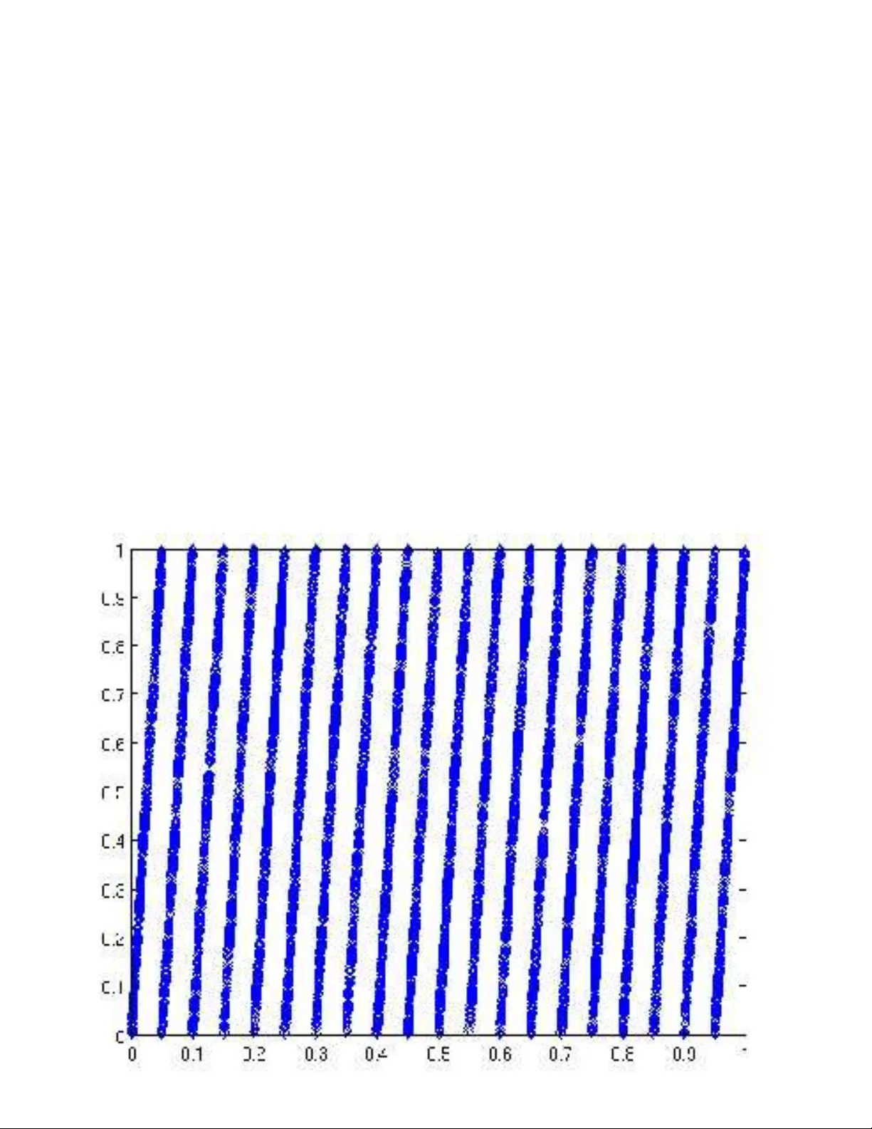
apport   de recherche ISSN 0249-6399 ISRN INRIA/RR--6391--FR+ENG Thème SYM INSTITUT N A TION AL DE RECHERCHE EN INFORMA TIQUE ET EN A UTOMA TIQUE T o wards P ersistence- Based Reconstruction in Euclidean Spaces Frédéric Chazal — Ste ve Y . Ou dot N° 6391 December 2007 Centre de recher che INRIA S aclay – Î le-de-Fran ce Parc Orsay Uni versité 4, rue Jacques Monod, 91893 ORSA Y Cedex Téléphone : +33 1 72 92 59 00 T o w ards P ersistence-Based Reconstruction in Euclidean Spaces F r´ ed ´ eric Chazal ∗ , Stev e Y. Oudot ∗ Th ` eme SYM — Syst ` emes sym b oliques ´ Equip e-Pro jet G ´ eometrica Rapp ort de rec herc he n ° 6391 — Dece mber 200 7 — 23 pages Abstract: Manifold reco nstru ction has b een extensiv ely studied among the computational geometry com- m unity for the last decade or so, esp ecially i n t wo and th r ee dimensions. Recen tly , signiﬁcan t impro ve ments w ere made in higher dimen sions, leading to new metho ds to r econstruct large classes of compact subsets of Eu clidean space R d . Ho wev er, the complexities of these method s scale u p ex- p onentia lly with d, w hic h mak es them impractical in medium or high dimensions, eve n for handling lo w-dimensional su b manifolds. In this pap er, we introduce a nov el approac h that s tand s in -b et we en reconstruction and top o- logica l estimation, and whose complexit y scales up with the in trinsic dimension of the data. Our algorithm com bines tw o paradigms: greedy reﬁnement, and top ological p ersistence. Sp eciﬁcally , giv en a p oint cloud in R d , the algorithm builds a set of landmarks iterativ ely , while main taining nested pairs of complexes, w h ose images in R d lie clo se to the data, and whose p ersistent homology ev en tually coincides with the one of the u nderlying sh ap e. When the data p oin ts are su ﬃcien tly densely samp led from a smo oth m -sub manifold of R d , our metho d retriev es th e homology of the submanifold in time a t most c ( m ) n 5 , where n is th e size of the i np u t and c ( m ) is a constan t d ep end- ing solely on m . It can also prov ably w ell handle a wide range of compact subsets of R d , though with w orse complexities. Along the w a y to pro ving the correctness of our algorithm, we obtain new r esults on ˇ Cec h, Rips, and witness complex ﬁltrations in Euclidean s p aces. Sp eciﬁcally , we show h ow previous r esults on unions of balls can b e transp osed to ˇ Cec h ﬁltrations. Moreo ve r, we p rop ose a simple framew ork for studying the prop erties of ﬁ ltrations that are in tert wined with th e ˇ Cec h ﬁltration, among whic h are the Rips and witness complex ﬁ ltrations. Finally , we in v estigate f urther on witness complexes and quan tify a conjecture of Carlsson and de Silv a, whic h states that witness complex ﬁ ltrations sh ould ha v e cleaner p ersistence b arco des than ˇ Cec h or Rip s ﬁltrations, at least on s mo oth subm anifolds of Euclidean spaces. Key-w ords: Reconstruction, Pe rsistent Homolog y , Fi ltration, ˇ Cec h complex, Rip s complex, Witness complex, T op ologica l estimation ∗ INRIA F uturs, Pa rc Orsay Un iversi t´ e, 4, ru e Jacques Monod - Bˆ at. P , 91893 O RSA Y Ce dex, F rance. { frederic .chazal, steve.oudot } @inria .fr V ers une reconstruction bas ´ ee sur la p ersistance d ans les espaces euclidiens R ´ esum ´ e : La r econstruction de v ari ´ et ´ es a ´ et ´ e fortemen t ´ etudi ´ ee durant cette d er n i ` ere d´ ecennie, en particulier dans le cas des p etites dimensions. Des a v anc ´ ees r ´ ecen tes d ans le cas des p lus grandes dimensions on t p ermis l’ ´ emergence de nou velles m ´ etho des de reconstru ction qui p euven t traiter des n uages de p oin ts issus de sous-v ari ´ et ´ es li sses de R d de dimensions arbitraires. T outefois, la complexit ´ e de ces appr o c hes cro ˆ ıt exp onen tiellemen t a v ec la dim en sion d de l’espace am bian t, ce qui les rend impraticables en dimensions mo y ennes ou grandes, meme p our reconstruire des sous- v ari ´ et ´ es de p etite dimension telles qu e des courb es ou d es su rfaces. Dans cet article, nous in tro duison une nouvell e appr o c he qui se situe ` a la front i ` ere entre la reconstruction classique et l’inf´ erence top ologique, et dont la complexit ´ e cro ˆ ıt a v ec la dimension in trins` eque des donn´ ees. Notre algorithme com bine deux paradigmes : le raﬃnement glouton type maxmin et la p ersistence top ologique. Plus pr ´ ecis´ emen t, ´ etan t donn´ e un nuage de p oints dans R d , l’algorithme construit un sous -ensem ble de landmarks it´ erative ment, tout en main tenan t une paire de complexes simp liciaux im briqu´ es, dont les images dans R d son t pr o c hes des donn´ ees, et dont l’homologie p ersistan te coincide a vec l’homologie de l’espace sous-jacen t aux d onn ´ ees. Quand le n uage de p oin t est suﬃsammen t d ens ´ emen t ´ ec h an tillonn ´ e ` a partir d ’une sous-v ari ´ et´ e lisse de R d , notre m ´ etho de r etrouve l’homologie d e la v ari ´ et ´ e en temps c ( m ) n 5 , o ` u n est la taill e d e l’en tr ´ ee et c ( m ) est u ne constante d´ ep endant uniquement de la dimen sion int rins` eque m de la v ari ´ et´ e. Notre appro che p eut aussi r econstru ire a v ec garan ties un e large classe d’ob jets compacts dans R d , av ec de m oins b ons temps de calcul toutefois. Aﬁn d e donner d es ga ranti es th ´ eoriques ` a not re alg orithme, nous ´ etudions l es ﬁltratio ns de ˇ Cec h, de Rips, et de complexes d e t ´ emoins dans R d , p our lesquels nous p r ´ esen tons un ensem ble de r´ esultats nouv eaux. Plus pr´ ecis ´ ement, nous mon trons commen t d es r ´ esu ltats existan ts su r les unions de b oules p euven t ˆ etre transf´ er ´ es aux ﬁltrations de ˇ Cec h, p uis de l` a aux ﬁltrations de Rips et de complexes de t´ emoins. Nous prop osons ´ egaleme nt u ne pr emi ` ere quantiﬁca tion d’un e conjecture de Carlss on et de Silv a, selon laquelle les ﬁltrations de complexes de t´ emoins fourn issen t de meilleurs r ´ esultats que les ﬁ ltrations de ˇ Cec h et de Rip s dans le cadre d e l’inf ´ erence top ologique, en tout cas p our le cas des sous-v ari ´ et ´ es lisses de R d . Mots-cl ´ es : Rec onstruction, Homologie p ersistante , Filtration, Complexe d e ˇ Cec h, C omplexe de Rips, Complex d e t ´ emoins, Inf ´ erence top ologique T owar ds P ersistenc e-Base d R e c onstruction in Euclide an Sp ac es 3 1 Int ro duction The problem of reconstructing u n kno wn structures fr om ﬁnite collect ions of data samples is ubiqui- tous in the Sciences, where it has man y diﬀeren t v arian ts, dep ending on the nature of the data and on the targeted application. In the last decade or so, the compu tational geometry communit y has gained a lot of interest in manifold reconstruction, where the goal is to reconstruct subm anifolds of Euclidean spaces from p oin t clouds. In particular, eﬃcien t solutions hav e b een prop osed in d imen- sions t wo and three, based on the use of the Delauna y triangulation – see [8] f or a survey . In these metho ds, th e u nknown manifold is app ro ximated by a simplicial complex that is extracted from the full-dimensional Delauna y triangulation of the input p oin t cloud. The s uccess of this app roac h is explained by th e f act that, not only do es it b ehav e w ell on pr actical examples, but the qualit y of its output is guarante ed by a sound theoretical framew ork. I ndeed, the extracted complex is usually sho wn to b e equal, or at least close, to the so-called r estricte d D elaunay triangulation , a particular subset of the Dela unay triangulation whose appro ximation p ow er is wel l-und ersto o d on smo oth or Lipschitz curve s an d surfaces [1, 2, 6]. Unfortu nately , the s ize of the Delauna y triangulation gro ws to o fast with the dimension of the am b ien t space for the approac h to b e still tractable in high-dimensional spaces [33]. Recen tly , signiﬁcan t steps were made tow ards a full und erstanding of the p otenti al and lim- itations of the restricted Delauna y triangulation on smo oth manifolds [14, 35]. In parallel, new sampling theories were devel opp ed, s uc h as t he critic al p oin t theory for distance functions [9], whic h pro vides s uﬃcien t conditions for the topology of a shap e X ⊂ R d to b e captured b y the oﬀsets of a p oin t cloud L lyin g at small Hausd orﬀ distance. These adv ances la y the foun d ations of a new theoretical fr amew ork for the reconstruction of smo oth submanifolds [11, 34], and more generally of large classes of compact subsets of R d [9, 10, 12]. Com bined with the in tro du ction of more ligh t w eigh t data structures, such as th e witness c omplex [16], they ha v e lead to new re- construction tec hniques in arbitrary Euclidean s p aces [4], wh ose outputs can b e guarante ed un der mild sampling conditions, and whose complexities can b e orders of magnitude b elo w the one of the classical Delauna y-based approac h. F or instance, on a data set with n p oints in R d , the algorithm of [4] runs in time 2 O ( d 2 ) n 2 , whereas the size of th e Delauna y triangulatio n can b e of the ord er of n ⌈ d 2 ⌉ . Unfortunately , 2 O ( d 2 ) n 2 still remains too large for these new metho ds to b e p ractical, ev en when the data p oin ts lie on or near a v ery lo w-dimensional submanifold. A we ak er yet similarly diﬃcult v ersion of the r econstruction p aradigm is top ological estimation, where the goal is not to exhibit a data structure that faithfully appro ximates the underlyin g sh ap e X , bu t simp ly to infer the topological in v arian ts of X f rom an input p oin t cloud L . This pr oblem has receiv ed a lot of atten tion in the recen t y ears, and it ﬁnds applications in a num b er of areas of Science, suc h as sensor netw orks [19 ], statistical analysis [7], or dyn amical systems [32, 36]. A classical approac h to learning the homology of X consists in building a nested sequence of spaces K 0 ⊆ K 1 ⊆ · · · ⊆ K m , and in studyin g the p ersistence of h omology classes throughou t this sequence. In particular, it has b een indep en den tly pr o v ed in [12] and [15] that the p ersistent homology of the sequence deﬁned by the α -oﬀsets of a p oin t cloud L coincides with the homology of the un derlying shap e X , under samp ling conditions that are milder than the ones of [9]. Sp eciﬁcally , if the Hausdorﬀ distance b et w een L and X is less than ε , for some small enough ε , then, for all α ≥ ε , the canonical inclusion map L α ֒ → L α +2 ε induces homomorphisms b et we en homology groups, whose images are isomorphic to the h omology groups of X . Combined with the structure th eorem of [38], whic h states that the p ersistent homology of the sequence { L α } α ≥ 0 is f u lly d escrib ed by a ﬁnite set of in terv als, called a p ersistenc e b ar c o de or a p ersistenc e diagr am — see Figure 1 (left), the ab o v e result means that th e h omology of X can b e d educed from this barcod e, simply b y remo ving the in terv als of length less than 2 ε , wh ic h are therefore viewed as top ological noise. RR n ° 6391 4 Chazal & Oudot F rom an algorithmic p oin t of v iew, th e p ersistent homology of a nested sequence of simplicial complexes (called a ﬁltr ation ) can b e eﬃcient ly computed using the p ersistence algorithm [22, 38]. Among the many ﬁltrations that can b e b uilt on top of a p oin t set L , the α -shap e enables to reliably reco v er the homology of the und erlying sp ace X , sin ce it is kno wn to b e a deformation retract of L α [21]. Ho wev er, th is prop erty is u seless in high d imensions, since computing the α -shap e requires to build the full-dimensional Delauna y triangulation. It is th er efore app ealing to consider other ﬁltrations that are easy to compute in arbitrary dimensions, su ch as the Rip s and witness complex ﬁltrations. Nev ertheless, to the b est of our knowledge , th ere curren tly exists no equiv alen t of the result of [12, 15] for suc h ﬁltrations. In this p ap er, we pro d uce suc h a result, not only for Rip s and witness complexes, bu t more generally for an y ﬁltration that is intert wined with the ˇ Cec h ﬁltration. Recall that, for all α > 0, the ˇ Cec h complex C α ( L ) is the nerve of the union of the op en balls of same radius α ab out the p oin ts of L , i.e. the nerve of L α . It follo ws fr om the nerv e theorem [31, Cor. 4G.3] that C α ( L ) and L α are h omotop y equ iv alen t. Ho wev er, despite the result of [12, 15], this is not suﬃ cien t to pro ve that the p ersistent h omology of C α ( L ) ֒ → C α +2 ε ( L ) coincides with the homology of X , mainly b ecause it is not clear whether the homotop y equiv alences C α ( L ) → L α and C α +2 ε ( L ) → L α +2 ε pro vided b y the n erv e th eorem commute w ith the ca nonical inclusions C α ( L ) ֒ → C α +2 ε ( L ) and L α ֒ → L α +2 ε . Using standard arguments of algebraic top ology , w e prov e that there exist some homotop y equ iv alences th at do comm ute with the canonical inclus ions , at least at homology and h omotop y lev els. T his enables us to extend the r esult of [12, 15] to the ˇ Cec h ﬁltration, and from there to the Rip s and w itness complex ﬁ ltrations. Figure 1: Results obtained from a set W of 10 , 000 p oin ts sampled un iformly at r andom f rom a helical curve dr awn on the 2d torus ( u, v ) 7→ 1 2 (cos 2 π u, sin 2 π u, cos 2 π v , sin 2 π v ) in R 4 — see [30]. Left: p ers istence barco de of the Rips ﬁltration, built o v er a set of 900 carefully-c hosen landmarks. Righ t: result of our algorithm, applied blindly to th e input W . Bot h metho ds h ighligh t the t wo underlying structures: curve and torus. Another common concern in top ological data analysis is th e size of the vertex s et on top of wh ic h a ﬁltration is bu ilt. In many practical situations ind eed, the p oint cloud W gi ve n as input samples the underlyin g sh ap e v ery ﬁnely . In su c h situations, it mak es sense to b uild the ﬁltration on top of a small subset L of landmarks, to a v oid a waste of computational resources. Ho w ev er, building a ﬁltration on top of the spars e landmark set L instead of the den se p oin t cloud W can result in a s igniﬁcan t degradation in th e qualit y of the p ersistence barco d e. Th is is true in particular with the ˇ Cec h and Rips ﬁltrations, whose barco des can ha ve top ological noise of amplitude dep endin g directly on the d ensit y of L . The introdu ction of the witness complex ﬁltration app eared as an elengan t wa y of solving this issue [18]. The witness complex of L relativ e to W , or C W ( L ) for INRIA T owar ds P ersistenc e-Base d R e c onstruction in Euclide an Sp ac es 5 short, can b e view ed as a relaxed v ersion of the Delauna y triangulation of L , in whic h the p oints of W \ L are used to driv e the construction of the complex [16]. Due to its sp ecial n atur e, wh ic h tak es adv ant age of the p oint s of W \ L , and due to its close relationship with the restricted Dela un ay triangulation, th e witness complex ﬁ ltration is lik ely to giv e p ersistence b arco des whose top ological noise dep ends on the densit y of W rather than on the one of L , as conjectured in [18]. W e pro v e in the p ap er that th is statemen t is only tru e to some exten t, namely: whenever the p oints of W are suﬃcien tly densely sampled from some smo oth su bmanifold of R d , the top ological noise in the barco de can b e arbitrarily small compared to the density of L . Nev ertheless, it cannot dep end solely on the den s it y of W . This sho ws that the witness complex ﬁ ltration do es pro vide cleaner p ersistence barco des than ˇ Cec h or Rips ﬁltrations, b ut ma yb e not as clea n as exp ected. T aking adv antage of th e ab o v e th eoretical r esults on Rips and w itn ess complexes, w e prop ose a nov el approac h to reconstruction that stands somewhere in -b et we en the classical reconstruction and top ological estimatio n paradigms. Ou r algorithm is a v ariant of th e metho d of [4, 30] th at com bines greedy reﬁnement and top ological p ersistence. Sp eciﬁcally , giv en an input p oint cloud W , the algorithm bu ilds a su bset L of landmarks iterativ ely , and in the mean time it main tains a nested pair of simplicial complexes (which happ en to b e Rips or witness complexes) and computes its p ersistent Betti num b ers. The outcome of the algorithm is the sequence of nested pairs main tained throughout the pr o cess, or r ather the d iagram of ev olution of their p ersistent Betti num b ers . Using this diagram, a user or softw are agen t can determine a relev an t scale at wh ic h to pro cess the data. It is then easy to rebu ild the corresp ond ing set of land marks, as w ell as its nested pair of complexes. Note that our metho d do es not completely solv e the classical reconstruction problem, since it d o es not exhibit an em b edd ed complex that is close to X top ologically and geometrically . Nev ertheless, it comes w ith theoretical guaran tees, it is easily implementa ble, and ab o v e all it has reasonable complexit y . In d eed, in the case wh ere the input p oin t cloud is sampled from a smo oth s u bmanifold X of R d , we s ho w that the complexit y of our algorithm is b ound ed by c ( m ) n 5 , w here c ( m ) is a quan tit y dep ending solely on the in trinsic dimension m of X , w hile n is the size of the input. T o the b est of our kn owledge, this is the ﬁrst pro v ably-go o d top ological estimation or reconstruction metho d w hose complexit y scales up with the intrinsic dimension of the m anifold. In the case w here X is a more general compact set in R d , our complexit y b ound b ecomes c ( d ) n 5 . The pap er is organized as follo w s: after introdu cing the ˇ Cec h, Rips, and witness complex ﬁltrations in S ection 2, we pro v e our stru ctural results in S ections 3 and 4, fo cusing on the general case of compact su bsets of R d in Section 3, and more sp eciﬁcally on the case of smo oth subm anifolds of R d in S ection 4 . Finally , we pr esen t our algorithm and its analysis in Section 5. 2 V arious complexes and their relationships The d eﬁ nitions, results and pro ofs of this section hold in an y arbitrary metric space. Ho wev er, for the sak e of consistency with the rest of the pap er, w e state them in the particular case of R d , endo w ed with the Euclidean norm k p k = q P d i =1 p 2 i . As a consequence, our b ounds are n ot the tigh test p ossible for the Eu clidean case, but they are for the general metric case. Using sp eciﬁc prop erties of Euclidean spaces, it is ind eed p ossible to w ork out somewhat tigh ter b ounds, b ut at the price of a loss of sim p licit y in the statement s. F or any compact s et X ⊂ R d , we call diam( X ) the diameter of X , and d iam CC ( X ) th e c omp onent-wise diameter of X , deﬁn ed b y: d iam CC ( X ) = inf i diam( X i ), where the X i are the path-connected comp onen ts of X . Finall y , giv en t w o compact sets X , Y in R d , we call d H ( X, Y ) their Hausd orﬀ d istance. RR n ° 6391 6 Chazal & Oudot ˇ Cec h c omplex. Giv en a ﬁnite set L of p oin ts of R d and a p ositiv e num b er α , w e call L α the union of the op en b alls of radius α cen tered at the p oin ts of L : L α = S x ∈ L B ( x, α ). This deﬁnition mak es sense only for α > 0, since for α = 0 we get L α = ∅ . W e also denote b y { L α } the op en co ver of L α formed b y the op en balls of r ad iu s α cen tered at the p oin ts of L . The ˇ Cec h complex of L of parameter α , or C α ( L ) for short, is the nerve of this cov er, i.e. it is th e abstract simplicial complex w hose vertex set is L , and suc h that, for all k ∈ N and all x 0 , · · · , x k ∈ L , [ x 0 , · · · , x k ] is a k -simplex of C α ( L ) if and only if B ( x 0 , α ) ∩ · · · ∩ B ( x k , α ) 6 = ∅ . Rips complex. Giv en a ﬁnite set L ⊂ R d and a p ositive num b er α , the Rips complex of L of parameter α , or R α ( L ) for short, is the abstract simp licial complex wh ose k -simp lices corresp ond to unord er ed ( k + 1)-tuples of p oin ts of L which are p airwise within Euclidean d istance α of one another. The Rips complex is closely relat ed to the ˇ Cec h complex, as stated in the follo w in g standard lemma, whose pro of is recalled for completeness: Lemma 2.1 F or al l ﬁnite se t L ⊂ R d and al l α > 0 , we have: C α 2 ( L ) ⊆ R α ( L ) ⊆ C α ( L ) . Pro of. The p ro of is standard. Let [ x 0 , · · · , x k ] b e an arbitrary k -simplex of C α 2 ( L ). Th e Euclidean balls of same radiu s α 2 cen tered at the x i ha v e a n on-empt y common intersectio n in R d . Let p b e a p oint in the intersectio n. W e then ha v e: ∀ 0 ≤ i, j ≤ k , k x i − x j k ≤ k x i − p k + k p − x j k ≤ α . T his implies that [ x 0 , · · · , x k ] is a s im p lex of R α ( L ), whic h prov es the ﬁ r st in clusion of the lemma. Let no w [ x 0 , · · · , x k ] b e an arbitrary k -simplex of R α ( L ). W e ha v e k x 0 − x i k ≤ α for all i = 0 , · · · , k . This means th at x 0 b elongs to all the Eu clidean balls B ( x i , α ), wh ic h therefore hav e a n on-empt y common in tersection in R d . It follo ws th at [ x 0 , · · · , x k ] is a simplex of C α ( L ), whic h pro v es the second inclusion of the lemma.  Witness complex. Let L b e a ﬁn ite su b set of R d , referred to as the landmark set, and let W b e another (p ossibly inﬁnite) sub set of R d , iden tiﬁed as the witness set. Let also α ∈ [0 , ∞ ). – Giv en a p oint w ∈ W and a k -simp lex σ with v ertices in L , w is an α -witness o f σ (or, equiv alen tly , w α -witnesses σ ) if the v ertices of σ lie within Euclidean d istance (d k ( w ) + α ) of w , wh ere d k ( w ) denotes the Euclidean distance b et w een w and its ( k + 1)th nearest landmark in th e Eu clidean m etric. – The α -witness c omplex of L r elative to W , or C α W ( L ) for short, is the maximum abstract simplicial complex, w ith vertic es in L , wh ose faces are α -witnessed by p oin ts of W . When α = 0, the α -witness complex coincides w ith the standard witness complex C W ( L ), int ro d uced in [17]. The α -witness complex is also closely related to the ˇ Cec h complex, though the relationship is a b it more su btle than in the case of the Rip s complex: Lemma 2.2 L et L , W ⊆ R d b e su c h that L i s ﬁnite. If every p oint o f L lie s within E uclide an distanc e l of W , then for al l α > l we h ave: C α − l 2 ( L ) ⊆ C α W ( L ) . In ad dition, if the Euclide an distanc e fr om any p oint of W to its se c ond ne ar est neighb or in L is at most l ′ , then f or al l α > 0 we have: C α W ( L ) ⊆ C 2( α + l ′ ) ( L ) . Pro of. Let [ x 0 , · · · , x k ] b e a k -simplex of C α − l 2 ( L ). Th is means that T k i =0 B ( x i , α − l 2 ) 6 = ∅ , and as a r esu lt, th at k x 0 − x i k ≤ α − l for all i = 0 , · · · , k . Let w b e a p oin t of W closest to x 0 in the Euclidean metric. By the h yp othesis of the lemma, w e ha ve k w − x 0 k ≤ l , therefore x 0 , · · · , x k lie within Euclidean distance α of w . Since the Euclidean d istances f rom w to its nearest p oin ts of L are non-negativ e, w is an α -witness of [ x 0 , · · · , x k ] and of all its faces. As a result, [ x 0 , · · · , x k ] is a simplex of C α W ( L ). INRIA T owar ds P ersistenc e-Base d R e c onstruction in Euclide an Sp ac es 7 Consider n o w a k -simplex [ x 0 , · · · , x k ] of C α W ( L ). If k = 0, then the simplex is a v ertex [ x 0 ], and therefore it b elongs to C α ′ ( L ) for all α ′ > 0. Assu me no w that k ≥ 1. Edges [ x 0 , x 1 ] , · · · , [ x 0 , x k ] b elong also to C α W ( L ), hence they are α -witnessed by p oin ts of W . Let w i ∈ W be an α -witness of [ x 0 , x i ]. Distances k w i − x 0 k and k w i − x i k are b oun ded f rom ab o v e b y d 2 ( w i ) + α , w here d 2 ( w i ) is the Euclidean distance from w i to its second nearest p oin t of L , whic h b y assumption is at most l ′ . It follo ws that k x 0 − x i k ≤ k x 0 − w i k + k w i − x i k ≤ 2 α + 2 l ′ . Since this is tru e for all i = 0 , · · · , k , w e conclude that x 0 b elongs to the inte rsection T k i =0 B ( x i , 2( α + l ′ )), whic h is therefore non-empt y . As a r esu lt, [ x 0 , · · · , x k ] is a s im p lex of C 2( α + l ′ ) ( L ).  Corollary 2.3 L et X b e a c omp act subset of R d , and let L ⊆ W ⊆ R d b e such that L i s ﬁnite. Assume that d H ( X, W ) ≤ δ and that d H ( W , L ) ≤ ε , with ε + δ < 1 4 diam CC ( X ) . Then, fo r al l α > ε , we have: C α − ε 2 ( L ) ⊆ C α W ( L ) ⊆ C 2 α +6( ε + δ ) ( L ) . In p articular, if δ ≤ ε < 1 8 diam CC ( X ) , then, for al l α ≥ 2 ε we have: C α 4 ( L ) ⊆ C α W ( L ) ⊆ C 8 α ( L ) . Pro of. S ince d H ( W , L ) ≤ ε , ev ery p oin t of L lies within Euclidean distance ε of W . As a r esult, the ﬁrst in clusion of Lemma 2.2 holds with l = ε , th at is: C α − ε 2 ( L ) ⊆ C α W ( L ). No w, for ev ery p oin t w ∈ W , there is a p oint p ∈ L suc h that k w − p k ≤ ε . More- o v er, there is a p oin t x ∈ X suc h that k w − x k ≤ δ , since we assumed that d H ( X, W ) ≤ δ . Let X x b e th e path-connected comp onen t o f X that c ont ains x . T ake an arbitrary v alue λ ∈  0 , 1 2 diam CC ( X ) − 2( ε + δ )  , and consider the op en ball B ( w , 2( ε + δ ) + λ ). This ball clearly in tersects X x , since it con tains x . F u r thermore, X x is not cont ained en tirely in the ball, since otherwise w e wo uld ha v e: d iam CC ( X ) ≤ diam( X x ) ≤ 4( ε + δ ) + 2 λ , hereby contradicti ng the fact that λ < 1 2 diam CC ( X ) − 2( ε + δ ). Hence, there is a p oint y ∈ X lyin g on the b ound in g sp here of B ( w , 2( ε + δ ) + λ ). Let q ∈ L b e closest to y . W e ha ve k y − q k ≤ ε + δ , since our hypothesis implies that d H ( X, L ) ≤ d H ( X, W ) + d H ( W , L ) ≤ δ + ε . It follo ws then from the triangle inequalit y that k p − q k ≥ k w − y k − k w − p k − k y − q k ≥ 2( ε + δ ) + λ − ( ε + δ ) − ( ε + δ ) = λ > 0. Thus, q is diﬀeren t from p , and therefore the b all B ( w, 3( ε + δ ) + λ ) con tains at least tw o p oin ts of L . Since this is true for arbitrarily small v alues of λ , th e Euclidean distance from w to its second n earest neigh b or in L is at most 3( ε + δ ). It follo ws that the second inclusion of Lemma 2.2 holds with l ′ = 3( ε + δ ), that is: C α W ( L ) ⊆ C 2( α +3( ε + δ )) ( L ).  As mentio ned at the head of the section, sligh tly tight er b ound s can b e wo rked out usin g sp eciﬁc prop erties of Euclidean s p aces. F or the case of the Rips complex, this w as d one by de Silv a and Ghrist [19, 27]. Their ap p roac h can b e combined with ours in the case of the witness complex. 3 S tru c tural prop erties of ﬁltrations o v er compact subsets of R d Throughout th is sectio n, w e use classical concepts of algebraic topology , such as homotop y equiv- alences, deformation r etracts, or singu lar homology . W e r efer the reader to [31] for a go o d intro- duction to these concepts. Giv en a compact set X ⊂ R d , w e den ote b y d X the distanc e function deﬁned b y d X ( x ) = inf {k x − y k : y ∈ X } . Alt hough d X is n ot d iﬀeren tiable, it is p ossible to deﬁne a notion of critical p oint for distance fu nctions and we denote b y wfs( X ) the we ak f e atur e size of X , d eﬁned as the smallest p ositiv e critica l v alue of the distance fu nction to X [10]. W e do not exp licitly u se the notion of critical v alue in the follo wing, but only its relationship with th e top ology of the oﬀsets X α = { x ∈ R d : d X ( x ) ≤ α } , stressed in the follo wing resu lt from [29]: RR n ° 6391 8 Chazal & Oudot Lemma 3.1 ( Isotop y Lemma) If 0 < α < α ′ ar e such that ther e is no critic al value of d X in the close d interval [ α, α ′ ] , then X α and X α ′ ar e home omorphic (and even isotopic), and X α ′ deformation r etr acts onto X α . In p articular the h yp othesis of th e lemma is satisﬁed when 0 < α 1 < α 2 < wfs( X ). In other w ords, all the oﬀsets of X ha v e th e same top ology in the in terv al (0 , wfs ( X )). 3.1 Results on homology W e use sin gular h omology with co eﬃcients in an arbitrary ﬁ eld – omitted in our notations. In the follo w ing, we rep eatedly m ak e use of the follo wing standard r esult of linear algebra: Lemma 3.2 ( Sandwic h L e mma) Consider th e fol lowing se q uenc e of homomorphisms b etwe en ﬁnite-dimensional ve ctor sp ac es over a same ﬁeld: A → B → C → D → E → F. Assu me that rank ( A → F ) = r ank ( C → D ) . Then, this quantity also e quals the r ank of B → E . In the same way, if A → B → C → E → F is a se quenc e of homomorp hisms such that r ank ( A → F ) = dim C , then r ank ( B → E ) = dim C . Pro of. Ob serv e that, f or an y sequence of homomorphisms F f → G g → H , w e ha v e rank ( g ◦ f ) ≤ min { rank f , r ank g } . Applying this fact to maps A → F , B → E , and C → D , which are nested in the sequ ence of the lemma, w e get: rank ( A → F ) ≤ ran k ( B → E ) ≤ r ank ( C → D ), whic h pro v es the ﬁ r st statement of the lemma. As for the s econd statement , it is obtained from the ﬁrst one by letting D = C and taking C → D to b e th e identit y map.  3.1.1 ˇ Cec h ﬁltra t ion Since the ˇ Cec h complex is the nerv e of a union of balls, its top ological inv arian ts can b e read from the s tr ucture of its dual union. It turn s out that unions of balls ha ve b een extensivel y stu died in the past [9, 12, 15]. Our analysis relies particularly on the follo wing result, wh ic h is an easy extension of Theorem 4.7 of [12]: Lemma 3.3 L et X b e a c omp act set and L a ﬁnite set in R d , such that d H ( X, L ) < ε for some ε < 1 4 wfs( X ) . Then, for al l α, α ′ ∈ [ ε, wfs( X ) − ε ] such that α ′ − α ≥ 2 ε , and for al l λ ∈ (0 , wf s ( X )) , we have: ∀ k ∈ N , H k ( X λ ) ∼ = im i ∗ , wher e i ∗ : H k ( L α ) → H k ( L α ′ ) is the homomorphism b e twe en homolo gy gr oups induc e d by the c anonic al inclusion i : L α ֒ → L α ′ . Given an arbitr ary p oint x 0 ∈ X , the same c onclusion holds for homo topy gr oups with b ase-p oint x 0 . Pro of. W e can assume without loss of generalit y that ε < α < α ′ − 2 ε < wfs( X ) − 3 ε , since otherwise w e can r eplace ε b y an y ε ′ ∈ ( d H ( X, L ) , ε ). F r om the h yp othesis w e deduce the follo wing sequence of in clusions: X α − ε ֒ → L α ֒ → X α + ε ֒ → L α ′ ֒ → X α ′ + ε (1) By the Isotop y Lemma 3.1, for all 0 < β < β ′ < wfs( X ), the canonical inclusion X β ֒ → X β ′ is a homotop y equiv alence. As a consequen ce, Eq. ( 1) ind uces a sequence of homomorphisms b et we en homology groups, suc h that all homomorphisms b et wee n homology groups of X α − ε , X α + ε , X α ′ + ε are isomorphism s. It follo ws then from the Sandwich Lemma 3.2 that i ∗ : H k ( L α ) → H k ( L α ′ ) has same r ank as these isomorp hisms. No w, this rank is equal to the dimension of H k ( X λ ), sin ce th e X β are homotop y equiv alen t to X λ for all 0 < β < wfs( X ). It follo ws that im i ∗ ∼ = dim H k ( X λ ), since our ring of coeﬃcien ts is a ﬁ eld. The case of h omotop y group s is a little tric kier, since replacing INRIA T owar ds P ersistenc e-Base d R e c onstruction in Euclide an Sp ac es 9 homology groups by homotop y group s do es n ot allo w u s to u s e th e ab ov e rank argument. Ho w ev er, w e can use the same pro of as in T heorem 4.7 of [12] to conclude.  Observe that Lemma 3.3 d o es not guaran tee the retriev al of the homology of X . I n stead, it deals with suﬃciently small oﬀsets of X , w hic h are homotop y equiv alen t to one another but p ossibly not to X itself. In the sp ecial case where X is a smo oth submanifold of R d ho w ev er, X λ and X are homotop y equiv alent, and therefore the theorem guaran tees the retriev al of the h omology of X . F rom an algorithmic p oin t of view, the main drawbac k of Lemma 3.3 is that compu tin g the homology of a union of balls or the image of the h omomorphism i ∗ is usually a wkwa rd. As men tionned in [12, 15] this can b e d one b y computing th e p ersistence of the α -shap e or λ -medial axis ﬁ ltrations asso ciated to L but there do not exist eﬃcient algorithms to compute these ﬁ ltrations in dimension more than 3. In the follo wing we sho w th at w e can still reliably obtain the homology of X from easier to compute ﬁltrations, namely the Rip s and Witness complexes ﬁltrations. Consider now the ˇ Cec h complex C α ( L ), for any v alue α > 0. By d eﬁnition, C α ( L ) is the n erv e of the op en co ver { L α } of L α . Since the elements of { L α } are op en E u clidean b alls, they are con v ex, and therefore their inte rsections are either e mpty or c on ve x. It follo ws that { L α } satisﬁes the h yp otheses of the nerve the or em , wh ic h implies that C α ( L ) and L α are homotop y equiv alen t – see e.g. [31, Corollary 4G.3]. W e thus get the follo wing diagram, where horizonta l arro ws are canonical inclusions, and v ertical arrows are homotop y equiv alences pro vided by the nerve theorem: L α ֒ → L α ′ ↑ ↑ C α ( L ) ֒ → C α ′ ( L ) (2) Determining whether this diagram comm utes is not straigh tforwa rd. The follo wing r esult, based on standard argum en ts of algebraic top ology , sho ws th at ther e exist homotop y equ iv alences b etw een the un ion of b alls and the ˇ Cec h complex that make the ab o v e diagram commutativ e at homology and homotop y lev els: Lemma 3.4 L et L b e a ﬁnite set of p oints in R d and let 0 < α < α ′ . Then, ther e exist homotop y e quivalenc es C α ( L ) → L α and C α ′ ( L ) → L α ′ such that, for al l k ∈ N , the diagr am of E q. (2) induc es the f ol lowing c ommutative diagr ams: H k ( L α ) → H k ( L α ′ ) π k ( L α ) → π k ( L α ′ ) ↑ ↑ and ↑ ↑ H k ( C α ( L )) → H k ( C α ′ ( L )) π k ( C α ( L )) → π k ( C α ′ ( L )) wher e vertic al arr ows ar e isomorphisms . Pro of. Our app r oac h consists in a quic k review of the pro of of the nerv e theorem pro vided in Section 4G of [31], and in a simple extension of the main argumen ts to our con text. As mentio ned earlier, the op en co v er { L α } satisﬁes the conditions of the nerve theorem, namely: for all p oint s x 0 , · · · , x k ∈ L , T k l =0 B ( x l , α ) is either empt y , or con ve x and therefore contract ible. F rom this co v er w e construct a top ologica l sp ace ∆ L α as follo ws: let ∆ n denote the stand ard n - simplex, where n = # L − 1. T o eac h non-empty subset S of L w e asso ciate the face [ S ] of ∆ n spanned by the elemen ts of S , as w ell as the space B S ( α ) = T s ∈ S B ( s, α ) ⊆ L α . ∆ L α is then the subspace of L α × ∆ n deﬁned b y: ∆ L α = [ ∅6 = S ⊆ L B S ( α ) × [ S ] RR n ° 6391 10 Chazal & Oudot The space ∆ L α ′ is built similarly . The pro du ct s tructures of ∆ L α and ∆ L α ′ imply the existence of canonica l p ro jections p α : ∆ L α → L α and p α ′ : ∆ L α ′ → L α ′ . These pr o jections comm ute with the canonical inclusions ∆ L α ֒ → ∆ L α ′ and L α ֒ → L α ′ , whic h implies that the follo wing d iagram: L α ֒ → L α ′ p α ↑ ↑ p α ′ ∆ L α ֒ → ∆ L α ′ (3) induces commutati ve d iagrams at homology and homotopy lev els. Moreo v er, sin ce { L α } is an op en co ver of L α , wh ic h is paracompact, p α is a homotop y equiv alence [31, Pr op. 4G.2 ]. Th e same holds for p α ′ , and therefore p α and p α ′ induce isomorphisms at h omology and homotop y lev els. W e no w sho w that, similarly , there exist homotopy equiv alences ∆ L α → C α ( L ) and ∆ L α ′ → C α ′ ( L ) that co mmute with the c anonical inclusions ∆ L α ֒ → ∆ L α ′ and C α ( L ) ֒ → C α ′ ( L ). This follo w s in fact from the p ro of of Corollary 4G.3 of [31]. Indeed, using the notion of c omplex of sp ac es int ro d uced in [31 , S ection 4G], it can b e sho wn that ∆ L α is the realization of the complex of spaces asso ciated with the cov er { L α } — see the p r o of of [31, Prop. 4G.2]. Its base is the barycen tric sub division Γ α of C α ( L ), where eac h v ertex corresp on d s to a non-empty ﬁn ite in tersection B S ( α ) for s ome S ⊆ L , and where eac h edge connecting t w o vertice s S ⊂ S ′ corresp onds to the canonical inclusion B S ′ ( α ) ֒ → B S ( α ). In the same wa y , ∆ L α ′ is the realization of a complex of sp aces b uilt o v er th e b arycen tric sub division Γ α ′ of C α ′ ( L ). No w, since the n on-empt y ﬁn ite intersecti ons B S ( α ) (resp. B S ( α ′ )) are con tractible, th e map q α : ∆ L α → Γ α (resp. q α ′ : ∆ L α ′ → Γ α ′ ) indu ced b y sending eac h op en set B S ( α ) (resp. B S ( α ′ )) to a p oint is a h omotop y equiv alence [31 , Prop. 4 G.1 and Corol. 4G.3]. F ur th ermore, by construction, q α is the r estriction of q α ′ to ∆ L α . Therefore, ∆ L α ֒ → ∆ L α ′ q α ↓ ↓ q α ′ Γ α ֒ → Γ α ′ (4) is a comm utativ e diagram where vertica l arrows are h omotop y equiv alences. No w, it is w ell-kno wn that Γ α and Γ α ′ are h omeomorphic to C α ( L ) an d C α ′ ( L ) r esp ectiv ely , and that the h omeomorphisms comm ute with the inclusion. Combined with (3) and (4), this fact prov es Lemma 3.4.  Com bining Lemmas 3.3 and 3.4, we obtain th e follo wing k ey result: Theorem 3.5 L et X b e a c omp act set and L a ﬁnite set in R d , such that d H ( X, L ) < ε for some ε < 1 4 wfs( X ) . Then, for al l α, α ′ ∈ [ ε, wfs( X ) − ε ] such that α ′ − α > 2 ε , and for al l λ ∈ (0 , wfs( X )) , we have: ∀ k ∈ N , H k ( X λ ) ∼ = im j ∗ , wher e j ∗ : H k ( C α ( L )) → H k ( C α ′ ( L )) is the homomo rphism b etwe e n homol o gy gr oups induc e d by the c anonic al inclusion j : C α ( L ) ֒ → C α ′ ( L ) . Given an arbitr ary p oint x 0 ∈ X , the same r esult holds for homotopy gr oups with b ase-p oint x 0 . Using the terminology of [38], this result means that the homology of X λ can b e dedu ced f r om the p ersistent homology of the ﬁltration {C α ( L ) } α ≥ 0 b y remo ving the cycles of p ersistence less than 2 ε . Equiv alen tly , the amplitude of the top olo gic al noise in the p ersistence barco de of {C α ( L ) } α ≥ 0 is b ound ed by 2 ε , i.e . th e in terv als of length at least 2 ε in the barco d e giv e the homology of X λ . 3.1.2 Filtrations intert wined with t he ˇ Cec h ﬁltra t ion Using Lemma 2.1 and Theorem 3.5, w e get the follo wing guarantee s on the Rips ﬁltration: Theorem 3.6 L et X ⊂ R d b e a c omp act set, and L ⊂ R d a ﬁnite set such that d H ( X, L ) < ε for some ε < 1 9 wfs( X ) . Then, for al l α ∈  2 ε, 1 4 (wfs( X ) − ε )  and al l λ ∈ (0 , wfs( X )) , we have: ∀ k ∈ N , H k ( X λ ) ∼ = im j ∗ , wher e j ∗ : H k ( R α ( L )) → H k ( R 4 α ( L )) is the homomorp hism b etwe en homolo gy gr oups induc e d by the c anonic al inclusion j : R α ( L ) ֒ → R 4 α ( L ) . INRIA T owar ds P ersistenc e-Base d R e c onstruction in Euclide an Sp ac es 11 Pro of. F rom Lemma 2.1 w e d educe th e follo wing sequence of inclusions: C α 2 ( L ) ֒ → R α ( L ) ֒ → C α ( L ) ֒ → C 2 α ( L ) ֒ → R 4 α ( L ) ֒ → C 4 α ( L ) (5) Since α ≥ 2 ε , Theorem 3.5 implies that Eq. (5) induces a sequence of homomorphisms b et w een homology groups, suc h that H k ( C α 2 ( L )) → H k ( C 4 α ( L )) and H k ( C α ( L )) → H k ( C 2 α ( L )) ha v e ranks equal to d im H k ( X λ ). Therefore, by the Sandwich Lemma 3.2, rank j ∗ is also equal to d im H k ( X λ ). It follo ws that im j ∗ ∼ = dim H k ( X λ ), since our ring of co eﬃcient s is a ﬁeld.  Similarly , Corollary 2.3 p ro vides the follo wing sequen ce of inclusions: C α 4 ( L ) ֒ → C α W ( L ) ֒ → C 8 α ( L ) ֒ → C 9 α ( L ) ֒ → C 36 α W ( L ) ֒ → C 288 α ( L ) , from whic h follo ws a result similar to Theorem 3.6 on the witness complex, by the same pro of: Theorem 3.7 L et X b e a c omp act subset of R d , and let L ⊆ W ⊆ R d b e such that L is ﬁnite. As- sume that d H ( X, W ) ≤ δ and that d H ( W , L ) ≤ ε , with δ ≤ ε < min  1 8 diam CC ( X ) , 1 1153 wfs( X )  . Then, for al l α ∈  4 ε, 1 288 (wfs( X ) − ε )  and al l λ ∈ (0 , wfs( X )) , we have: ∀ k ∈ N , H k ( X λ ) ∼ = im j ∗ , wher e j ∗ : H k ( C α W ( L )) → H k ( C 36 α W ( L )) is the homomor phism b etwe en homolo gy g r oups induc e d by the c anonic al inclusion j : C α W ( L ) ֒ → C 36 α W ( L ) . More generally , the ab o v e argumen ts s ho w th at the homology of X λ can b e reco v ered from the p ersistence b arco de of any ﬁltration { F α } α ≥ 0 that is in tert wined with the ˇ Cec h ﬁltration in the sense of Lemmas 2.1 and 2.2. Note ho we ve r th at Th eorems 3.6 and 3.7 suggest a diﬀeren t b eha vior of the barco de in this case, since its top ologica l noise might scale up w ith α (sp eciﬁcally , it might b e up to linear in α ), whereas it is un iformly b ounded b y a constan t in the case of the ˇ Cec h ﬁltration. This diﬀerence of b ehavi or is easily explained by the w a y { F α } α ≥ 0 is in tert wined with th e ˇ Cec h ﬁltration. A tric k to get a u niformly-b ounded noise is to repr esen t the barco de of { F α } α ≥ 0 on a logarithmic scale, that is, with log 2 α ins tead of α in ab cissa. 3.2 Results on homotop y The results on homology obtained in S ection 3.1 follo w from sim p le algebraic argumen ts. Using a more geometric approac h, w e can get similar results on homotop y . F rom n o w on, x 0 ∈ X is a ﬁxed p oint and all the homotop y group s π k ( X ) = π k ( X, x 0 ) are assumed to b e with base-p oint x 0 . Theorems 3.6 and 3.7 can b e extended to homotopy in the f ollo w in g wa y: Theorem 3.8 Under the same hyp otheses as in The or em 3.6, we have: ∀ k ∈ N , π k ( X λ ) ∼ = im j ∗ , wher e j ∗ : π k ( R α ( L )) → π k ( R 4 α ( L )) is the homomorphism b e twe en homotopy gr oups induc e d by the c anonic al inclusion j : R α ( L ) ֒ → R 4 α ( L ) . Theorem 3.9 Under the same hyp otheses as in The or em 3.7, we have: ∀ k ∈ N , π k ( X λ ) ∼ = im j ∗ , wher e j ∗ : π k ( C α W ( L )) → π k ( C 36 α W ( L )) is the homomo rphism b etwe en hom otopy gr oups induc e d by the c anonic al inclusion j : C α W ( L ) ֒ → C 36 α W ( L ) . The p ro ofs of these t wo results b eing m ostly identi cal, we fo cus exclusiv ely on the Rips complex. W e will use the follo wing lemma, w hic h is an immediate generalization of Pr op osition 4.1 of [12]: Lemma 3.10 L et X b e a c omp act set and L a ﬁnite set in R d , such that d H ( X, L ) < ε for some ε < 1 4 wfs( X ) . L et α, α ′ ∈ [ ε, wfs( X ) − ε ] b e such that α ′ − α ≥ 2 ε . Given k ∈ N , two k-lo ops σ 1 , σ 2 : S k → ( L α , x 0 ) in L α ar e homotop ic in X α ′ + ε if and only if they ar e homotop ic in L α ′ . RR n ° 6391 12 Chazal & Oudot Pro of of Theorem 3.8 . As men tionned at th e b egining of the pro of of Lemma 3.3, we can assume without loss of generalit y that 2 ε < α < 1 4 (wfs( X ) − ε ). Consider the follo wing sequence of inclusions: C α 2 ( L ) ⊂ R α ( L ) ⊂ C α ( L ) ⊂ C 2 α ( L ) ⊂ R 4 α ( L ) ⊂ C 4 α ( L ) W e use the homotop y equiv alences h β : L β → C β ( L ) pro vided by Lemma 3.4 for all v alues β > 0, whic h comm ute with inclusions at homotopy lev el. Note that, for an y elemen t σ of π k ( C β ( L )), there exists a k -lo op in L β that is mapp ed through h β to a k -lo op representing th e homotop y class σ . In the follo wing, we denote b y σ g suc h a k -lo op. Let E , F a nd G b e the images of π k ( C α 2 ( L )) in π k ( C α ( L )), π k ( C 2 α ( L )) and π k ( C 4 α ( L )) resp ectiv ely , th r ough the homomorphisms induced by inclusion. W e thus hav e a sequence of sur jectiv e homomorphisms: π k ( C α 2 ( L )) → E → F → G Note that, b y Theorem 3.5, F and G are isomorph ic to π k ( X λ ). Let σ ∈ F b e a homotopy class. Since F is the image of π k ( C α 2 ( L )), we can assume without loss of generali t y that σ g ⊂ L α 2 . Assume that the image of σ in G is equal to 0. This means that σ g is null-homot opic in L 4 α and, sin ce L 4 α ⊂ X 4 α + ε , σ g is also null- homotopic in X 4 α + ε . But σ g ⊂ L α 2 ⊂ X α 2 + ε , and X 2 α + ε deformation retracts onto X α 2 + ε , by the Isotop y Lemma 3.1. As a consequen ce, σ g is n ull-homotopic in X α 2 + ε , wh ic h is con tained in L 2 α since α 2 + 2 ε < 2 α . Hence, σ g is null-homotopic in L 2 α , n amely: σ = 0 in F . So, the homomorph ism F → G is injectiv e, and th us it is an isomorphism. As a consequence, F → π k ( R 4 α ( L )) is injectiv e, and it is n o w suﬃcient to pro v e that the image of φ ∗ : π k ( R α ( L )) → π k ( C 2 α ( L )) in duced by th e inclusion is equal to F . Ob viously , F is con tained in the image of φ ∗ . No w, let σ ∈ π k ( R α ( L )) and let φ ∗ ( σ ) g b e a k -lo op in L 2 α that is mapp ed through h 2 α to a k -lo op r epresent ing the homotop y class φ ∗ ( σ ). Since φ ∗ ( σ ) is in th e image of φ ∗ , and since R α ( L ) ⊂ C α ( L ), we can assum e that φ ∗ ( σ ) g is cont ained in L α . Let ˜ σ g b e the image of φ ∗ ( σ ) g through a d eformation retraction of X 2 α + ε on to X α 0 , where 0 < α 0 < α 2 is su c h that α 2 − α 0 > ε . Obvio usly , ˜ σ g and φ ∗ ( σ ) g are homotopic in X 2 α + ε . It follo w s then from Lemma 3.1 0 that ˜ σ g and φ ∗ ( σ ) g are homotopic in L 2 α . An d since ˜ σ g is con tained in X α 0 ⊂ L α 2 , the equiv alence class of h α 2 ( ˜ σ g ) in π k ( C α 2 ( L )) is mapp ed to φ ∗ ( σ ) ∈ π k ( C 2 α ( L )) through the homomorphism induced by C α 2 ( L ) ֒ → C 2 α ( L ), w h ic h comm utes with the homotopy equiv alences. As a r esu lt, φ ∗ ( σ ) b elongs to F , which is therefore equal to im φ ∗ .  4 T he c ase of smo oth submanifolds of R d In this section, we consider the case of su bmanifolds X of R d that hav e p ositiv e r e ach . Recall that the reac h of X , or rc h( X ) for short, is the m inim um d istance b et w een the p oin ts of X and the p oints of its m edial axis [1]. A p oin t cloud L ⊂ X is an ε -samp le of X if ev ery p oint of X lies within distance ε of L . In ad d ition, L is ε -sp arse if its p oints lie at least ε a w a y from one another. Our main result is a ﬁrst att empt at quantifying a conjecture of C arlsson and de Silv a [18], according to whic h the witness complex ﬁltration sh ould ha v e cle aner p ersistence barco des than the ˇ Cec h and Rips ﬁ ltrations, at least on smo oth sub m anifolds of R d . By cle aner is mean t that the amp litude of the top ologica l noise in the barco des should b e smaller, and also that the long in terv als shou ld app ear earlier. W e p ro v e this latter statemen t correct, at least to some exten t: Theorem 4.1 Ther e exist a c onstant  > 0 and a c ontinuous, non-de cr e asing map ¯ ω : [0 ,  ) → [0 , 1 2 ) , such that, for any submanifold X of R d , for al l ε, δ satisfying 0 < δ ≤ ε <  rch( X ) , for any δ - sample W of X and any ε -sp arse ε -sample L of W , C α W ( L ) c ontains a sub c omplex D home omorph ic INRIA T owar ds P ersistenc e-Base d R e c onstruction in Euclide an Sp ac es 13 to X and such that the c anonic al inclusion D ֒ → C α W ( L ) induc es an i nje ctive homomorhism b etwe en homolo gy gr oups, pr ovide d that α satisﬁes: 8 3 ( δ + ¯ ω ( ε rch( X ) ) 2 ε ) ≤ α < 1 2 rc h( X ) − (3 + √ 2 2 )( ε + δ ) . This theorem guarante es that, f or v alues of α ranging from O ( δ + ¯ ω ( ε rch( X ) ) 2 ε ) to Ω(rc h ( X )), the top ology of X is captured by a sub complex D that injects itself suitably in C α W ( L ). As a result, long in terv als sho wing the h omology of X app ear around α = O ( δ + ¯ ω ( ε rch( X ) ) 2 ε ) in the p ersistence barco de of the witness complex ﬁltration. Th is can b e muc h so oner than the time α = 2 ε prescrib ed b y Theorem 3.7, since ¯ ω ( ε rch( X ) ) can b e arbitrarily s m all. Sp eciﬁcally , the denser the landmark set L , the smaller the ratio ε rch( X ) , and therefore the smaller δ + ¯ ω ( ε rch( X ) ) 2 ε compared to 2 ε . W e ha ve reasons to b eliev e that this u pp er b ound on the app earance time of long bars is tigh t. In particular, the b ound cannot dep end solely on δ , since otherwise, in the limit case where δ = 0, we w ould get that the homology grou p s of X can b e injected into the ones of th e standard witn ess complex C W ( L ), which is known to b e f alse [30, 35]. The same argument implies th at th e amplitude of the top ological n oise in the b arco de cannot dep end solely on δ either. How ev er, whether the upp er b ound O ( ε ) on the amplitude of the noise can b e improv ed or not is still an op en question. Our pro of of Theorem 4.1 generalizes and argument u sed in [26] for the planar case, whic h stresses th e close relatio nsh ip that exists b et w een the α -witness complex and the so-called weighte d r estricte d Delaunay triangulation D X ω ( L ). Giv en a su bmanifold X of R d , a ﬁ nite land mark set L ⊂ R d , and an assignment of non-n egativ e we igh ts to the landmarks, sp eciﬁed through a map ω : L → [0 , ∞ ), D X ω ( L ) is the n erv e of the r estriction to X of the p ower diagr am 1 of the w eigh ted set L . Under the hyp otheses of the theorem, we show that C α W ( L ) con tains D X ω ( L ), whic h, b y a result of Cheng et al. [14] (see Th eorem 4.2 b elo w), is homeomorphic to X . The main p oint of the pro of is then to s h o w that D X ω ( L ) injects itself nic ely into C α W ( L ). The rest of th e section is devot ed to the p ro of of T heorem 4.1. After introd ucing th e w eigh ted restricted Delaunay triangulation in Section 4.1 and stressing its r elationship with the α -witness complex in S ection 4.2, w e detail the pro of of Theorem 4.1 in Section 4.3. 4.1 The w eigh ted r estricted Delauna y triangulation Giv en a ﬁn ite p oin t set L ⊂ R d , an assignment of weights over L is a non-negativ e real-v alued function ω : L → [0 , ∞ ). The quantit y max u ∈ L,v ∈ L \{ u } ω ( u ) k u − v k is calle d the r elative amplitude of ω . Giv en p ∈ R d , the weighte d distanc e from p to some w eigh ted p oin t v ∈ L is k p − v k 2 − ω ( v ) 2 . This is actually n ot a metric, since it is not sy m metric. Giv en a ﬁ nite p oin t set L and an assignment of w eigh ts ω o v er L , w e d enote by V ω ( L ) the p o w er diagram of th e w eigh ted set L , and by D ω ( L ) its nerv e, also known as the we ight ed Delauna y triangulation. If the relativ e amplitude of ω is at most 1 2 , then the p oin ts of L hav e non-empty cells in V ω ( L ), and in fact eac h p oint of L b elongs to its o wn cell [13]. F or an y simplex σ of D ω ( L ), V ω ( σ ) d enotes the face of V ω ( L ) dual to σ . Giv en a subset X of R d , w e call V X ω ( L ) the restriction of V ω ( L ) to X , and w e denote b y D X ω ( L ) its nerv e, also kno wn as the wei ghte d Delauna y triangulation of L restricted to X . Ob serv e that D X ω ( L ) is a sub complex of D ω ( L ). In the sp ecial case wh ere all the w eigh ts are equal, V ω ( L ) and D ω ( L ) coincide with their standard Eu clidean ve rsions, V ( L ) and D ( L ). Similarly , V ω ( σ ) b ecomes V( σ ), and V X ω ( L ) and D X ω ( L ) b ecome r esp ectiv ely V X ( L ) and D X ( L ). Theorem 4.2 ( Lemmas 13, 14, 18 of [14], see also Theorem 2.5 of [4]) Ther e exist 2 a c on- stant  > 0 and a non-de cr e asing c ontinuous map ¯ ω : [0 ,  ) → [0 , 1 2 ) , such that, for any manifold 1 More on p ow er diagrams an d on restricted triangulations can be found in [3] and [23] respectively . 2 Note that  and ¯ ω are the same as in Theorem 4.1. In fact, these quantiti es come from Theorem 4.2. RR n ° 6391 14 Chazal & Oudot X and any ε -sp arse 2 ε -samp le L of X , with ε <  rc h( X ) , ther e is an assignment of weights ω of r elative amplitude at most ¯ ω  ε rch( X )  such that D X ω ( L ) is home omorphic to X . This theorem guaran tees that the top ology of X is captured by D X ω ( L ) p ro vided that the landmarks are suﬃcien tly densely sampled on X , and that they are assigned suitable w eigh ts. Observe that the denser the landmark set, the sm aller the weigh ts are requir ed to b e, as sp eciﬁed by the map ¯ ω . In th e particular case w here X is a curve or a su rface, ¯ ω can b e tak en to b e the constan t zero map, since D X ( L ) is homeomorphic to X [1, 2]. On higher-dimensional manifolds though, p ositiv e w eigh ts are r equired, since D X ( L ) ma y fail to capture the top ological inv ariants of X [35]. The pr o of of the theorem give n in [14] sh o ws th at V X ω ( L ) satisﬁes the so-called close d b al l pr op erty , whic h states that ev ery face of the w eigh ted V oronoi d iagram V ω ( L ) inte rsects the manifold X along a top ological ball of prop er d imension, if at all. Under th is condition, there exists a homeomorphism h 0 b et wee n the ner ve D X ω ( L ) and X , as pro v ed b y Edelsbr unner and Shah [23]. F urtherm ore, h 0 sends ev ery simplex of D X ω ( L ) to a subset of the union of the restricted V oronoi cells of its v ertices, that is: ∀ σ ∈ D X ω ( L ), h 0 ( σ ) ⊆ S v v ertex of σ V ω ( v ) ∩ X . This f act will b e instrumental in the p ro of of T heorem 4.1 . 4.2 Relationship b etw een D X ω ( L ) and C α W ( L ) As men tioned in in tro d u ction, the use of the witness complex ﬁ ltration for top ological data analysis is motiv ated b y its close relationship w ith th e weig hte d restricted Delauna y triangulation: Lemma 4.3 L et X b e a c omp act subset of R d , W ⊆ X a δ -sample of X , and L ⊆ W an ε -sp arse ε -sample of W . Then, f or al l assignment of weights ω of r elative amplitude ¯ ω ≤ 1 2 , D X ω ( L ) is include d in C α W ( L ) whenever α ≥ 2 1 − ¯ ω 2  δ + ¯ ω 2 ε  . This resu lt im p lies in particular that D X ( L ) is included in C α W ( L ) when ev er α ≥ 2 δ , since D X ( L ) is n othing but D X ω ( L ) for an assignmen t of weig hts of relativ e amp litude zero. Pro of. Let σ b e a simp lex of D X ω ( L ). If σ is a vertex, then it clearly b elongs to C α W ( L ) for all α ≥ 0, since L ⊆ W . Assume no w that σ has p ositiv e dimension, and consider a p oin t c ∈ V ω ( σ ) ∩ X . F or any vertex v of σ and any p oint p of L (p ossib ly equal to v ), we h a v e: k v − c k 2 − ω ( v ) 2 ≤ k p − c k 2 − ω ( p ) 2 , whic h yields: k v − c k 2 ≤ k p − c k 2 + ω ( v ) 2 − ω ( p ) 2 . No w , ω ( p ) 2 is n on-negativ e, while ω ( v ) 2 is at most ¯ ω 2 k v − p k 2 , wh ic h giv es: k v − c k 2 ≤ k p − c k 2 + ¯ ω 2 k v − p k 2 . Replacing k v − p k by k v − c k + k p − c k , w e get a semi-algebraic expression of degree 2 in k v − c k , n amely: (1 − ¯ ω 2 ) k v − c k 2 − 2 ¯ ω 2 k p − c kk v − c k − (1 + ¯ ω 2 ) k p − c k 2 ≤ 0 . It follo ws that k v − c k ≤ 1+ ¯ ω 2 1 − ¯ ω 2 k p − c k . Let no w w b e a p oin t of W closest to c in th e Eu clidean metric. Using the triangle inequalit y and the fact that k w − c k ≤ δ , w e get: k v − w k ≤ k v − c k + k w − c k ≤ 1+ ¯ ω 2 1 − ¯ ω 2 k p − c k + δ . This holds for an y p oint p ∈ L , and in particular for the nearest neigh b or p w of w in L . Th erefore, w e ha v e k v − w k ≤ 1+ ¯ ω 2 1 − ¯ ω 2 k p w − c k + δ , whic h is at most 1+ ¯ ω 2 1 − ¯ ω 2 ( k p w − w k + δ ) + δ ≤ k p w − w k + 2 1 − ¯ ω 2  δ + ¯ ω 2 ε  b ecause k w − c k ≤ δ and k w − p w k ≤ ε . Since this inequalit y holds for an y vertex v of σ , and since the Eu clidean distances from w to all the landmarks are at least k p w − w k , w is an α -witness of σ and of all its f aces as so on as α ≥ 2 1 − ¯ ω 2  δ + ¯ ω 2 ε  . Since this holds for ev ery simplex σ of D X ω ( L ), the lemma follo ws.  4.3 Pro of of Theorem 4.1 The pro of is mostly algebraic, but it relies on t w o tec hnical results. The ﬁrst one is Dugundj i’s extension theorem [20], w h ic h states that, give n an abstract simplex σ and a con tinuous map INRIA T owar ds P ersistenc e-Base d R e c onstruction in Euclide an Sp ac es 15 f : ∂ σ → R d , f can b e extend ed to a conti nuous map f : σ → R d suc h that f ( σ ) is includ ed in the Eu clidean conv ex h ull of f ( ∂ σ ), noted CH( f ( ∂ σ )). This conv exit y p rop erty of f is used in th e pro of of the second technical resu lt, stated as Lemma 4.5 an d p ro v ed at the end of the section. Pro of of Theorem 4.1. Since δ ≤ ε , L is an ε -spars e 2 ε -sample of X , with ε <  rc h( X ). Therefore, by Theorem 4.2, there exists an assignmen t of w eigh ts ω o v er L , of relativ e amplitude at most ¯ ω  ε rch( X )  , suc h that D X ω ( L ) is homeomorphic to X . T aking D = D X ω ( L ), we then ha v e: ∀ k ∈ N , H k ( X ) ∼ = H k ( D ). Moreo ve r, by Lemma 4.3, w e k n o w that D = D X ω ( L ) is included in C α W ( L ), since α ≥ 8 3  ¯ ω  ε rch( X )  2 ε + δ  ≥ 2 1 − ¯ ω “ ε rc h ( X ) ” 2  ¯ ω  ε rch( X )  2 ε + δ  . There remains to sho w that the inclusion map j : D X ω ( L ) ֒ → C α W ( L ) ind uces injectiv e homomorph isms j ∗ b et wee n the homology groups of D X ω ( L ) and C α W ( L ), whic h will conclude the pro of of the theorem. Our approac h to sh owing the in j ectivit y of j ∗ consists in build ing a conti nuous m ap 3 h : C α W ( L ) → D X ω ( L ) suc h that h ◦ j is homoto pic to the identit y in D X ω ( L ). T his implies th at h ∗ ◦ j ∗ : H k ( D X ω ( L )) → H k ( D X ω ( L )) is an isomorphism (in fact, it is the identit y map), and thus that j ∗ is injectiv e. W e b egin our construction with th e h omeomorphism h 0 : D X ω ( L ) → X pro vided by the theorem of Edelsbr unner and Shah [23]. T aking h 0 as a map D X ω ( L ) → R d , w e extend it to a cont inuous map ˜ h 0 : C α W ( L ) → R d b y the follo wing iterativ e p ro cess: while there exists a simp lex σ ∈ C α W ( L ) suc h that ˜ h 0 is d eﬁned ov er the b ound ary of σ bu t not o ver its inte rior, app ly Dugund ji’s extension theorem, whic h extends ˜ h 0 to th e entire simp lex σ . Lemma 4.4 The ab ove iter ative pr o c ess e xtends h 0 to a map ˜ h 0 : C α W ( L ) → R d . Pro of. W e only need to p ro v e that the p ro cess visits ev ery s implex of C α W ( L ). Assum e for a con trad iction that the pro cess termin ates while there still remain some un visited simplices of C α W ( L ). Consider one suc h simplex σ of minimal dimension. Either σ is a v er tex, or there is at least one p rop er face of σ that has n ot y et b een visited – sin ce otherwise the pro cess could visit σ . In the form er case, σ is a p oin t of L , and as such it is a ve rtex 4 of D X ω ( L ), whic h means that h 0 is already deﬁned o v er σ (con tradiction). In the latter case, w e get a con tradiction w ith the fact that σ is of minimal d imension.  No w that we h a v e built a map ˜ h 0 : C α W ( L ) → R d , our next step is to turn it into a map C α W ( L ) → X . T o do so, w e comp ose it with th e pro jection p X that m aps ev ery p oint of R d to its nearest n eigh b or on X , if the latte r is unique. This pro jection is k n o wn to b e w ell-deﬁned and con tin uous ov er R d \ M, where M den otes the medial axis of X [24]. Lemma 4.5 L et X, W, L, δ , ε satisfy the hyp otheses of The or em 4.1. Then, ˜ h 0 ( C α W ( L )) ∩ M = ∅ as long as α < 1 2 rc h( X ) −  3 + √ 2 2  ( ε + δ ) . Since by L emm a 4.5 w e ha v e ˜ h 0 ( C α W ( L )) ∩ M = ∅ , the map p X ◦ ˜ h 0 : C α W ( L ) → X is w ell-deﬁned and con tin uous. Ou r ﬁnal step is to comp ose it with h − 1 0 , to get a cont inuous map h = h − 1 0 ◦ p X ◦ ˜ h 0 : C α W ( L ) → D X ω ( L ). The restriction of h to D X ω ( L ) is simp ly h − 1 0 ◦ p X ◦ h 0 , which coincides with h − 1 0 ◦ h 0 = id since h 0 ( D X ω ( L )) = X . It follo w s that h ◦ j is h omotopic to the iden tit y in D X ω ( L ) (in fact, it is the iden tit y), and therefore that the induced map h ∗ ◦ j ∗ is the identit y . Th is implies that j ∗ : H k ( D X ω ( L )) → H k ( C α W ( L )) is inj ectiv e, whic h concludes th e pro of of Theorem 4.1.  3 Note that this map does not n eed to b e simplicial, since w e are using singular homology . 4 Indeed, every p oint p ∈ L lies on X and b elongs to its own cell, since ω has relativ e amp litu d e less th an 1 2 . Therefore, V ω ( p ) ∩ X 6 = ∅ , which means that p is a vertex of D X ω ( L ). RR n ° 6391 16 Chazal & Oudot W e end the section by providing the pro of of Lemma 4.5: Pro of of Lemma 4.5. First, we claim that the image through ˜ h 0 of any simp lex of C α W ( L ) is included in the Euclidean con v ex h ull of the restricted V oronoi cells of its simplices, that is: ∀ σ ∈ C α W ( L ), ˜ h 0 ( σ ) ⊆ CH ( S v v ertex of σ V ω ( v ) ∩ X ). This is clearly true if σ b elongs to D X ω ( L ), since in this case we ha v e ˜ h 0 ( σ ) = h 0 ( σ ) ⊆ S v v ertex of σ V ω ( v ) ∩ X , as menti oned after Th eorem 4.2. No w, if the prop ert y holds f or all th e prop er faces of a simplex σ ∈ C α W ( L ), then by in- duction it also holds for the simplex itself. In deed, for eac h pr op er face τ ⊂ σ , w e hav e ˜ h 0 ( τ ) ⊆ CH ( S v v ertex of τ V ω ( v ) ∩ X ) ⊆ CH ( S v v ertex of σ V ω ( v ) ∩ X ). Th erefore, CH ( S v v ertex of σ V ω ( v ) ∩ X ) con tains C H  ˜ h 0 ( ∂ σ )  , whic h, b y Dugundji’s extension theorem, con tains ˜ h 0 ( σ ). Therefore, th e prop erty holds for ev ery simplex of C α W ( L ). W e can now p ro v e that the image through ˜ h 0 of an y arbitrary simplex σ of C α W ( L ) do es not in tersect the medial axis of X . This is clea rly true if σ is a s implex of D X ω ( L ), since in this case ˜ h 0 ( σ ) = h 0 ( σ ) is included in X . Assu m e no w that σ / ∈ D X ω ( L ). In p articular, σ is not a verte x. Let v b e an arbirtary v er tex of σ . Consid er any other vertex u of σ . Edge [ u, v ] is α -witnessed b y some p oint w uv ∈ W . W e then ha v e k v − u k ≤ k v − w uv k + k w uv − u k ≤ 2d 2 ( w uv )+ 2 α , wh ere d 2 ( w uv ) stands for the Euclidean distance from w uv to its second nearest landmark. Acco rdin g to Lemma 3.4 of [4], w e ha v e d 2 ( w ) ≤ 3( ε + δ ), since L is an ( ε + δ )-sample of X . Thus, all th e v ertices of σ are included in the Euclidean ball B ( v , 2 α + 6( ε + δ )). Moreo v er, for any v ertex u of σ and any p oin t p ∈ V ω ( u ) ∩ X , w e hav e k p − u ′ k ≤ ε + δ , where u ′ is a landmark closest to p in the Eu clidean metric. Combined with the fact that k p − u k 2 − ω ( u ) 2 ≤ k p − u ′ k 2 − ω ( u ′ ) 2 , we get: k p − u k 2 ≤ k p − u ′ k 2 + ω ( u ) 2 ≤ 2( ε + δ ) 2 , since b y Lemma 3.3 of [4] w e ha v e ω ( u ) ≤ 2 ¯ ω  ε rch( X )  ( ε + δ ) ≤ ε + δ . Hence, V ω ( u ) ∩ X is included in B ( u, √ 2( ε + δ )) ⊂ B ( v , 2 α + (6 + √ 2)( ε + δ )). S ince this is true for ev ery v er tex u of σ , w e get: ˜ h 0 ( σ ) ⊆ CH ( S u vertex of σ V ω ( u ) ∩ X ) ⊆ B ( v , 2 α + (6 + √ 2)( ε + δ )). No w, v b elongs to L ⊆ W ⊆ X , and b y assu m ption we ha v e 2 α + (6 + √ 2)( ε + δ ) < rc h( X ), therefore ˜ h 0 ( σ ) do es not in tersect the medial axis of X .  5 A pplication to reconstruction T aking adv an tage of the str u ctural r esults of Section 3, we devise a very simple y et p ro v ably-go o d algorithm for constructing n ested pairs of complexes that can capture the h omology of a large class of compact su bsets of R d . This algorithm is a v arian t of the greedy reﬁnement tec hnique of [30], whic h b u ilds a set L of landmark s iterativ ely , and in the meantime maintai ns a suitable data structure. In our case, the d ata stru cture is comp osed of a nested p air of simplicial complexes, wh ic h can b e either R α ( L ) ֒ → R α ′ ( L ) or C α W ( L ) ֒ → C α ′ W ( L ), for s p eciﬁc v alues α < α ′ . Both v arian ts of the algorithm can b e used in arbitrary metric sp aces, with similar theoretica l guaran tees, although the v arian t u sing witness complexes is lik ely to b e more eﬀectiv e in practice. In the sequ el we fo cus on the v arian t using Rips complexes b ecause its analysis is somewhat simpler. 5.1 The algorithm The input is a ﬁ nite p oint set W d ra wn from an arbitrary metric space, toge ther with the pairwise distances l ( w, w ′ ) b etw een the p oin ts of W . In the sequel, W is iden tiﬁed as the set of witnesses. Initially , L = ∅ and ε = + ∞ . A t eac h iteratio n, the p oint of W lying f urthest a wa y 5 from L in the metric l is inserted in L , and ε is set to max w ∈ W min v ∈ L l ( w , v ). Th en, R 4 ε ( L ) and R 16 ε ( L ) are up dated, and the p ersistent homology of R 4 ε ( L ) ֒ → R 16 ε ( L ) is computed u sing the p ersistence 5 At the ﬁrst iteration, since L is empty , an arbitrary p oint of W is chosen. INRIA T owar ds P ersistenc e-Base d R e c onstruction in Euclide an Sp ac es 17 algorithm [38]. The algorithm terminates when L = W . T he output is the diagram sho wing the ev olution of the p ersisten t Betti n umb er s v ers u s ε , which ha v e b een mainta ined throughout th e pro cess. As we will see in Section 5.2 b elo w, with the help of th is diagram the user can determine a relev an t scale at which to pro cess the data: it is th en easy to generate the corresp onding sub set L of landmarks (the p oin ts of W ha v e b een sorted according to their order of insertion in L du ring the pro cess), and to rebuild R 4 ε ( L ) and R 16 ε ( L ). Th e pseudo-co d e of the algorithm is giv en in Figure 2. Input: W ﬁn ite, together with distances l ( w , w ′ ) for all w , w ′ ∈ W . Init: Let L := ∅ , ε := + ∞ ; While L ( W do Let p := argmax w ∈ W min v ∈ L l ( w , v ); // p chosen arbitr arily in W if L = ∅ L := L ∪ { p } ; ε := max w ∈ W min v ∈ L l ( w , v ); Up date R 4 ε ( L ) and R 16 ε ( L ); Compute p ersistent homology of R 4 ε ( L ) ֒ → R 16 ε ( L ); End while Output: diagram sho wing the ev olution of p ersistent Betti n umber s v ersus ε . Figure 2: Pseudo-co de of the algorithm. 5.2 Guaran t ees on the output F or any i > 0, let L ( i ) and ε ( i ) denote resp ectiv ely L and ε at th e end of th e i th iteratio n of the main loop of the algorithm. S ince L ( i ) kee ps gro wing w ith i , ε ( i ) is a decreasing fu nction of i . In addition, L ( i ) is an ε ( i )-sample of W , by deﬁnition of ε ( i ). Hence, if W is a δ -sample of some compact set X ⊂ R d , then L ( i ) is a ( δ + ε ( i ))-sample of X . Th is quantit y is less than 2 ε ( i ) whenev er ε ( i ) > δ . Therefore, Th eorem 3.6 provides us with the follo wing theoretical gu arantee: Theorem 5.1 Assume that the input p oint set W is a δ - sample of some c omp act set X ⊂ R d , with δ < 1 18 wfs( X ) . Then, at e ach iter ation i such that δ < ε ( i ) < 1 18 wfs( X ) , the p ersistent homolo gy gr oups of R 4 ε ( i ) ( L ( i )) ֒ → R 16 ε ( i ) ( L ( i )) ar e isomorphic to the homo lo gy gr oups of X λ , for al l λ ∈ (0 , wfs ( X )) . This theorem ensures that, when the input p oin t cloud W is su ﬃcien tly densely sampled fr om a compact s et X , there exists a r an ge of v alues of ε ( i ) suc h that the p ersistent Betti n um b ers of R 4 ε ( i ) ( L ( i )) ֒ → R 16 ε ( i ) ( L ( i )) coincide with the ones of suﬃcien tly small oﬀsets X λ . This means that a plateau app ears in the diagram of p ersistent Betti num b ers, sho wing th e Bet ti num b ers of X λ . In view of Theorem 5.1, th e width of th e plateau is at least 1 18 wfs( X ) − δ . The theorem also tells where the plateau is lo cated in the diagram, b ut in practice this do es not help since neither δ nor wfs( X ) are kno w n. How eve r, w hen δ is small enough compared to wfs( X ), the plateau is large enough to b e detected (and th us the homolog y of small oﬀsets of X inferred ) b y the user or a soft w are agent. In cases where W samples s everal compact sets with diﬀerent weak feature sizes, Theorem 5.1 ensures th at sev eral plateaus app ear in the diagram, showing p lausible reconstructions at v arious scales – see Figure 1 (r igh t). These guarante es are similar to the ones pr ovided w ith the lo w-dimensional version of the algorithm [30]. Once one or m ore p lateaus ha v e b een detected, the user can choose a relev ant scale at which to pro cess the data: as mentio ned in S ection 5.1 ab o v e, it is then easy to generate the corresp onding RR n ° 6391 18 Chazal & Oudot set of landmarks and to rebuild R 4 ε ( L ) and R 16 ε ( L ). Diﬀeren tly from the algorithm of [30], the outcome is not a single emb edded simp licial complex, but a nested pair of abstract complexes whose images in R d lie at Hausdorﬀ distance 6 O ( ε ) of X , su ch th at the p ersistent homology of the nested pair coincides w ith the homology of X λ . 5.3 Up date of R 4 ε ( L ) and R 16 ε ( L ) W e will no w describ e h ow to main tain R 4 ε ( L ) and R 16 ε ( L ). I n fact, we will settle for describing ho w to rebu ild R 16 ε ( L ) completely at eac h iteration, w hic h is suﬃ cient for ac hieving our complexity b ound s. In p ractice, it w ould b e m uc h p referable to use more lo cal rules to u p d ate the simplicial complexes, in order to a v oid a complete rebu ild ing at eac h iteration. Consider the one-sk eleton graph G of R 16 ε ( L ). The v ertices of G are the p oin ts of L , and its edges are the sets { p, q } ⊆ L suc h that k p − q k ≤ 16 ε . No w, b y d eﬁnition, a simplex that is not a ve rtex b elongs to R 16 ε ( L ) if and only if all its edges are in R 16 ε ( L ). Therefore, the simplices of R 16 ε ( L ) are precisely the cliques of G . The simplicial complex can then b e built as follo ws: 1. b uild graph G , 2. ﬁ nd all maximal cliques in G , 3. r ep ort the maximal cliques and all their su b cliques. Step 1. is p erformed w ithin O ( | L | 2 ) time b y c hecking the d istances b et we en all pairs of landm arks. Here, | G | d enotes the size of G and | L | the size of L . T o p er f orm Step 2., we u se the output-sensitiv e algorithm of [37], whic h ﬁn ds all the maximal cliques of G in O ( k | L | 3 ) time, where k is the size of the an s w er. Finally , r ep orting all the sub cliques of the maximal cliques is d one in time linear in the total n umb er of cliques, wh ich is also th e size of R 16 ε ( L ). Therefore, Corollary 5.2 At e ach iter ation of the algorithm, R 4 ε ( L ) and R 16 ε ( L ) ar e r ebuilt within O ( |R 16 ε ( L ) | | L | 3 ) time, wher e |R 16 ε ( L ) | i s the size of R 16 ε ( L ) and | L | the size of L . 5.4 Running time of the algorithm Let | W | , | L | , |R 16 ε ( L ) | denote the sizes of W, L, R 16 ε ( L ) resp ectiv ely . A t eac h iteration, p oin t p and parameter ε are computed naively b y iterating ov er the witnesses, and for eac h witness, b y reviewing its distances to all th e landmarks. This pro cedure tak es O ( | W || L | ) time. According to Corollary 5.2, R 4 ε ( L ) and R 16 ε ( L ) are up dated (in fact, rebuilt) in O ( |R 16 ε ( L ) || L | 3 ) time. Finally , the p ersistence algorithm runs in O ( |R 16 ε ( L ) | 3 ) time [22, 38]. Hence, Lemma 5.3 The running time of one iter ation of the algorithm is O ( | W || L | + |R 16 ε ( L ) || L | 3 + |R 16 ε ( L ) | 3 ) . There remains to ﬁ nd a r easonable b ou n d on the size of R 16 ε ( L ), which can b e done in Eu clidean space R d , esp ecially when the landmarks lie on a smo oth submanifold: Lemma 5.4 L et L b e a ﬁnite ε -sp arse p oint se t in R d . Then, R 16 ε ( L ) has at most 2 33 d | L | simplic es. If in addition the p oints of L lie on a smo oth m -submanifold X of R d with r e ach rc h( X ) > 16 ε , then R 16 ε ( L ) has at most 2 35 m | L | simplic es. Pro of. Giv en an arbitrary p oin t v ∈ L , we w ill sho w that the n umber of vertice s in the star of v in R 16 ε ( L ) is at most 33 d . F rom this follo ws that the num b er of simp lices in the s tar of v is b oun ded b y 2 33 d , which pro v es the ﬁr st part of the lemma. Let Λ b e the set of vertice s in the 6 Indeed, every simplex of R 16 ε ( L ) has all its vertices in X ε + δ ⊆ X 2 ε , and th e lengths of its edges are at most 16 ε . INRIA T owar ds P ersistenc e-Base d R e c onstruction in Euclide an Sp ac es 19 star of v . Th ese v ertices lie w ithin Euclidean distance 16 ε of v , and at least ε a w a y from one another. It follo ws that they are cen ters of pairwise-disjoint Euclidean d -balls of same radius ε 2 , included in the d -ball of cente r v and radiu s (16 + 1 2 ) ε . Therefore, their num b er is b ounded by v ol B ( v , (16+ 1 / 2 ) ε ) v ol B ( v , ε / 2 ) =  16+ 1 / 2 1 / 2  d = 33 d . Assume n o w that v and the p oin ts of Λ lie on a smo oth m -su bmanifold X of R d , suc h that 16 ε < rc h( X ). It follo ws then fr om Lemma 6 of [28] that, for all u ∈ Λ, we hav e k u − u ′ k ≤ k u − v k 2 2rc h( X ) ≤ ε 2 2rc h( X ) < ε 32 , where u ′ is the orthogonal p ro jection of u on to the tangen t sp ace of X at v , T ( v ). As a consequence, the orthogonal p ro jections of the p oint s of Λ on to T ( v ) lie at lea st 31 ε 32 a w a y fr om one another, and still at most 16 ε a w a y from v . As a result, th ey are cen ters of pairwise-disjoin t op en m -balls of same radius 31 ε 64 , in cluded in the op en m -ball of cen ter v and radiu s  16 + 31 64  ε inside T ( v ). Therefore, their num b er is b oun ded by  16+ 31 / 64 31 / 64  m ≤ 35 m , which pr o v es the second part of the lemma, by the same argumen t as ab o v e.  In cases where the in put p oin t cloud W lies on a sm o oth m -su bmanifold X of R d , th e ab o v e result 7 suggests that the course of the algorithm goes through t wo phases: ﬁrst, a transition p hase, in whic h the landmark set L is too coarse f or the dim en sionalit y of X to ha v e an inﬂ uence on the s hap es and sizes of the s tars of th e vertices of R 16 ε ( L ); second, a stable phase, in whic h the landmark set is d ense enough for the dimensionalit y of X to p la y a r ole. Th is f act is quite intuitiv e: imagine X to b e a simp le clo sed cur v e, embedd ed in R d in suc h a wa y th at it roughly ﬁlls in the space within the unit d -ball. T h en, for large v alues of ε , the landmark set L is nothing but a sampling of the d -ball, and therefore the stars of its p oin ts in R 16 ε ( L ) are d -dimensional. Let i 0 b e the last iteration of the transition phase, i. e . the last iteration suc h that ε ( i 0 ) ≥ 1 16 rc h( X ). Then, Lemmas 5.3 and 5.4 imply that the time complexit y of the transition phase is O ( | W || L ( i 0 ) | 2 + 8 33 d | L ( i 0 ) | 5 ), wh ile th e one of of the s table phase is O (8 35 m | W | 5 ). W e can get r id of the terms d ep ending on d in at least tw o w a ys: • The ﬁrst approac h has a rather theoretical ﬂav or: it consists in amortizing the cost of the transition phase by assuming that W is suﬃcien tly large. Sp eciﬁcally , since L ( i 0 ) is an ε ( i 0 )-sparse sample of X , with ε ( i 0 ) ≥ 1 16 rc h( X ), the size of L ( i 0 ) is b ound ed from ab o v e b y some quantit y c 0 ( X ) that dep ends solely on the (smo oth) manifold X – see e.g. [5] for a pro of in the sp ecial case of smo oth surf aces. As a result, we h a v e 8 33 d | L ( i 0 ) | k ≤ 8 35 m | W | k for all k ≥ 1 w henev er | W | ≥ 8 33 d − 35 m c 0 ( X ). Th is condition on the size of W translates into a condition on δ , b y a similar argumen t to the one inv ok ed ab ov e. • T he second app roac h has a more algorithmic ﬂav or, and it is based on a bac ktrac king strategy . Sp eciﬁcally , w e ﬁ r st r u n the algorithm without maintai ning R 4 ε ( L ) and R 16 ε ( L ), whic h simply sorts the p oints of W according to their order of insertion in L . Then, we run the algorithm bac kw ards, starting with L = L ( | W | ) = W and considering at eac h iteration j th e landmark set L ( | W | − j ). During this second p hase, we do maint ain R 4 ε ( L ) and R 16 ε ( L ) and compu te their p ers istent Betti n umb er s . If W samples X densely en ough, then T h eorem 5.1 ensures that the relev an t plateaus will b e computed b efore the transition p hase starts, and thus b efore the size of the d ata stru cture b ecomes indep en d en t of the dimension of X . It is then u p to the user to stop the pro cess wh en the space complexit y b ecomes to o large. In b oth cases, w e get the f ollo wing complexit y b ound s : 7 Note th at, at every iteration i of th e algorithm, L ( i ) is an ε ( i )-sparse p oint set, since the algorithm alwa ys inserts in L the p oin t of W lying furthest a w ay from L — see e.g. [30, Lemma 4.1]. RR n ° 6391 20 Chazal & Oudot Theorem 5.5 If W is a p oint cloud in Euc lide an sp ac e R d , then the running time of the algorithm is O (8 33 d | W | 5 ) , wher e | W | denotes the size of W . If in addition W is a δ - sample of some smo oth m -submanifold of R d , with δ smal l enough, then the running time b e c omes O (8 35 m | W | 5 ) . 6 Conclus ion This pap er mak es eﬀectiv e th e approac h d ev elopp ed in [12, 15] by pro viding an eﬃcien t, prov- ably go o d and easy-to-implemen t algorithm for top ological estimation of general shap es in any dimensions. Our theoretical framew ork can also b e u sed for the an alysis of other p ersistence-based metho ds. Addressing a weak er version of the classical reconstruction problem, w e in tro du ce an algorithm that ultimately outputs a nested pair of complexes at a user-deﬁn ed scale, from which the homology of the un derlying sh ap e X are inferred. When X is a smo oth submanifold of R d , the complexit y scales up w ith the intrinsic dimension of X . These results p ro vide a new step to w ards reconstructing (lo w-d imensional) manifolds in high-dimensional spaces in reasonnable time with top ological guaran tees. It is now tempting to tac kle the more c hallenging problem of constructing an em b edd ed simplicial complex that is top ologica lly and geometrically close to the sampled sh ap e. As a ﬁ rst step, w e in tend to adapt our metho d to pro vide a s in gle output complex that has the same homology as X , using for instance the se aling technique of [25]. References [1] N. Amen ta and M. Bern. Su rface reconstruction by V oronoi ﬁltering. Disc r ete Comput. Ge om. , 22(4): 481–504, 1999. [2] N. Amen ta, M. Bern, and D. Epp stein. T h e crus t and the β -ske leton: Com binatorial curv e reconstruction. Gr aphic al Mo dels and Image Pr o c essing , 60:125–1 35, 1998. [3] F. Aurenhammer. V oronoi d iagrams: A s urve y of a fund amen tal geometric d ata structure. ACM Comput. Surv. , 23(3):3 45–405, Septem b er 1991. [4] J .-D. Boissonnat, L. J. Guibas, and S. Y. Oudot. Manifold reconstruction in arbitrary di- mensions u sing witness complexes. In Pr o c. 23r d ACM Symp os. on Comput. Ge om. , pages 194–2 03, 2007. [5] J .-D. Boissonnat and S. Oudot. Pro v ably go o d samp lin g and meshing of surfaces. Gr aphic al Mo dels , 67(5):40 5–451, S ep tem b er 2005. [6] J .-D. Boissonnat and S. Oudot. Prov ably go o d sampling and meshin g of Lipsc hitz surfaces. In Pr o c. 22nd Annu. Symp os. Comput. Ge om. , p ages 337–346, 2006. [7] G. Carlsson, T. Ishkh ano v, V. de Silv a, and A. Zomoro dian. O n the lo cal b ehavio r of sp aces of natur al images. International Journal of Computer Vision , J u ne 2007. [8] F. Cazals and J. Giesen. Delauna y triangulation based surface reconstruction. In J.D. Bois- sonnat and M. T eillaud, editors, Eﬀe ctive Computationa l Ge ometry for Curves and Surfac es , pages 231–2 73. Springer, 2006. [9] F. Chazal, D. C ohen-Steiner, and A. Lieutier. A sampling theory for compact sets in Eu clidean space. In Pr o c. 22nd Annu. ACM Symp os. Comput. Ge om. , pages 319–326, 2006. INRIA T owar ds P ersistenc e-Base d R e c onstruction in Euclide an Sp ac es 21 [10] F. Ch azal and A. Lieutier. The λ -medial axis. Gr aphic al Mo dels , 67(4):304– 331, Ju ly 2005. [11] F. Ch azal and A. Lieutier. T op ology guaran teeing manifold reconstruction using distance function to noisy data. In P r o c. 22nd Annu. Symp os. on Comput. Ge om. , p ages 112–118 , 2006. [12] F. Chazal and A. Lieutier. Stabilit y and computation of top ological in v ariant s of solids in R n . Discr ete Comput. Ge om. , 37(4):6 01–617, 2007. [13] S.-W. C heng, T. K. Dey , H. Edelsb runn er , M. A. F acello, and S.-H. T eng. Sliv er exudation. Journal of the A CM , 47(5):88 3–904, 2000. [14] S.-W. Chen g, T. K. Dey , and E. A. Ramos. Ma nifold reconstru ction from p oin t samples. In Pr o c. 16th Symp os. Discr ete Algo rithms , pages 1018–10 27, 2005. [15] D. Cohen-Steiner, H. Edelsbr unner, and J. Harer. Stabilit y of p ersistence diagrams. In Pr o c. 21st A CM Symp os. Comput. Ge om. , pages 263–271 , 2005. [16] V. de Silv a. A w eak deﬁnition of Delauna y triangulation. T ec hnical r ep ort, S tanford Universit y , Octob er 2003. [17] V. d e Silv a. A w eak c haracterisation of th e Delauna y triangulation. Su bmitted to Ge ometriae De dic ata , 2007. [18] V. de Silv a and G. Carlsson. T op ological estimation using witness complexes. In Pr o c. Symp os. Point-Base d Gr aphics , pages 157–166 , 2004. [19] V. de S ilv a and R. Ghr ist. Co v erage in sensor n et w orks via p ersistent homology . Algebr aic & Ge ometric T op olo gy , 7:339–35 8, 2007. [20] J. Dugund ji. An extension of Tietze’s theorem. Paciﬁc J. Math. , 1:353–36 7, 1951. [21] H. Edelsbrunn er. The union of balls and its dual shap e. Discr ete Comput. Ge om. , 13:415– 440, 1995. [22] H. Edelsbru nner, D. Letsc her, and A. Z omoro dian. T op ological p ersistence and sim p liﬁcation. Discr ete Comput. Ge om. , 28:511 –533, 2002. [23] H. Ed elsb runn er and N. R . Shah. T riangulating top ological spaces. Int. J. on Comp. Ge om. , 7:365– 378, 1997 . [24] H. F ederer. Curv ature measures. T r ans. Amer. Math. So c. , 93:418–491 , 1959. [25] D. F reedman and C. Chen. Measuring and lo calizing homology classes. T ec hn ical Rep ort, Rensselaer P olytec h nic In stitute, Ma y 2007. [26] J. Gao, L. J . Gu ib as, S. Y. Oud ot, and Y. W ang. Geo desic Delauna y triangulations and witness complexes in the plane. In Pr o c. ACM-SIAM Symp os. Discr ete Algorith ms , 2008. [27] R Ghrist. Barco d es: The p ers istent top ology of data. Bul l. Amer. Math. So c. , Octob er 2007. [28] J. Giesen and U. W agner. S hap e dimension and in trinsic m etric from samples of manifolds with high co-dimension. Discr ete and Comp utational Ge ometry , 32:245 –267, 2004. RR n ° 6391 22 Chazal & Oudot [29] K. Gro v e. Critical p oin t theory for d istance fu nctions. In Pr o c. of Symp osia in Pu r e M athe- matics , volume 54, 1993. Part 3. [30] L. G. Gu ibas and S. Y. Oudot. Reconstru ction u sing witness complexes. In Pr o c. 18th Symp os. on D iscr ete Algorith ms , pages 1076–1 085, 2007. [31] A. Hatc her. Algebr aic T op olo gy . Cam brid ge Universit y Press, 2001. [32] T. Kaczynski, K. Mischai ko w, and M. Mrozek. Computational Homolo gy . Num b er 157 in Applied Mathematica l Sciences. Springer-V er lag, 200 4. [33] P . McMullen. T h e maximal num b er of faces of a conv ex p olytop e. Mathematika , 17:179–1 84, 1970. [34] P . Niy ogi, S. Smale, and S. W ein b erger. Find ing the homology of su bmanifolds with high conﬁdence f rom r andom samples. Discr ete Comput. Ge om. , to app ear. [35] S. Y. Oudot. On the top ology of the r estricted Delauna y triangulation and witness complex in higher dimensions. Man uscript. Preprint a v ailable at http://g eometry. stanford.edu/member/oudot/drafts/Delaunay_hd.pdf , No v em b er 2006. [36] V. Robins . T o w ards computing homology fr om appr o ximations. T op olo gy , 24:503–5 32, 1999. [37] S. Tsukiy ama, M. Id e, H. Ariyoshi, and I. Sh irak a wa . A n ew algorithm for generati ng all the maximal in dep end en t sets. SIAM J. on Computing , 6:505–517 , 1977. [38] A. Zomoro dian and G. Carlsson. Computing p ersistent homology . Discr ete Comput. Ge om. , 33(2): 249–274, 2005. INRIA T owar ds P ersistenc e-Base d R e c onstruction in Euclide an Sp ac es 23 Con ten ts 1 I n tro duction 3 2 V arious complexes and their relat ionships 5 3 St ructural prop ert ies of ﬁltrations o v er compact subsets of R d 7 3.1 Results on homology . . . . . . . . . . . . . . . . . . . . . . . . . . . . . . . . . . . . 8 3.1.1 ˇ Cec h ﬁltration . . . . . . . . . . . . . . . . . . . . . . . . . . . . . . . . . . . 8 3.1.2 Filtrations in tert wined with the ˇ Cec h ﬁltration . . . . . . . . . . . . . . . . . 10 3.2 Results on homotop y . . . . . . . . . . . . . . . . . . . . . . . . . . . . . . . . . . . . 11 4 T he case of smo oth submanifolds of R d 12 4.1 The w eigh ted restricted Delauna y triangulatio n . . . . . . . . . . . . . . . . . . . . . 13 4.2 Relationship b et w een D X ω ( L ) and C α W ( L ) . . . . . . . . . . . . . . . . . . . . . . . . . 14 4.3 Pro of of Theorem 4.1 . . . . . . . . . . . . . . . . . . . . . . . . . . . . . . . . . . . . 14 5 Application to re construction 16 5.1 The algorithm . . . . . . . . . . . . . . . . . . . . . . . . . . . . . . . . . . . . . . . . 16 5.2 Guaran tees on the outpu t . . . . . . . . . . . . . . . . . . . . . . . . . . . . . . . . . 17 5.3 Up d ate of R 4 ε ( L ) and R 16 ε ( L ) . . . . . . . . . . . . . . . . . . . . . . . . . . . . . . 18 5.4 Runn ing time of the algorithm . . . . . . . . . . . . . . . . . . . . . . . . . . . . . . 18 6 C onclusion 20 RR n ° 6391 Centre de recherche INRIA Saclay – Île-de-Fran ce Parc Orsay Uni versité - ZA C des V ignes 4, rue Jacques Monod - 9189 3 Orsay Cedex (France) Centre de recherc he INRIA Bordeaux – Sud Ouest : Domaine Univ ersitaire - 351, cours de la Libération - 33405 T alenc e Cedex Centre de recherc he INRIA Grenobl e – Rhône-Alpes : 655, avenu e de l’Europ e - 38334 Montbonnot Saint-Ismier Centre de recherc he INRIA Lille – Nord Europe : Pa rc Scientiﬁque de la Haute Borne - 40, avenu e Hall ey - 59650 V illene uve d’Ascq Centre de recherc he INRIA Nanc y – Grand Est : L ORIA, T echnopôle de Nancy-Bra bois - Campus scientiﬁque 615, rue du Jardin Botani que - BP 101 - 54602 V illers-lès-Na ncy Cede x Centre de recherc he INRIA Pari s – Rocquencourt : Domaine de V oluceau - Rocquencourt - BP 105 - 78153 L e Chesna y Ced ex Centre de recherc he INRIA Renne s – Bretagne Atlantique : IRISA, Campus univ ersitaire de Beaulieu - 35042 Rennes Cedex Centre de recherc he INRIA Sophia Antipolis – Méditerranée : 2004, route des Lucioles - BP 93 - 06902 Sophia Antipolis Cedex Éditeur INRIA - Domaine de V olucea u - Rocquenc ourt, BP 105 - 78153 Le Chesnay Cede x (France) http://www.inria.fr ISSN 0249 -6399

Towards Persistence-Based Reconstruction in Euclidean Spaces

Original Paper

Comments & Academic Discussion

Leave a Comment

Original Paper

Related Papers

Comments & Academic Discussion

Leave a Comment