Stability of the Gibbs Sampler for Bayesian Hierarchical Models

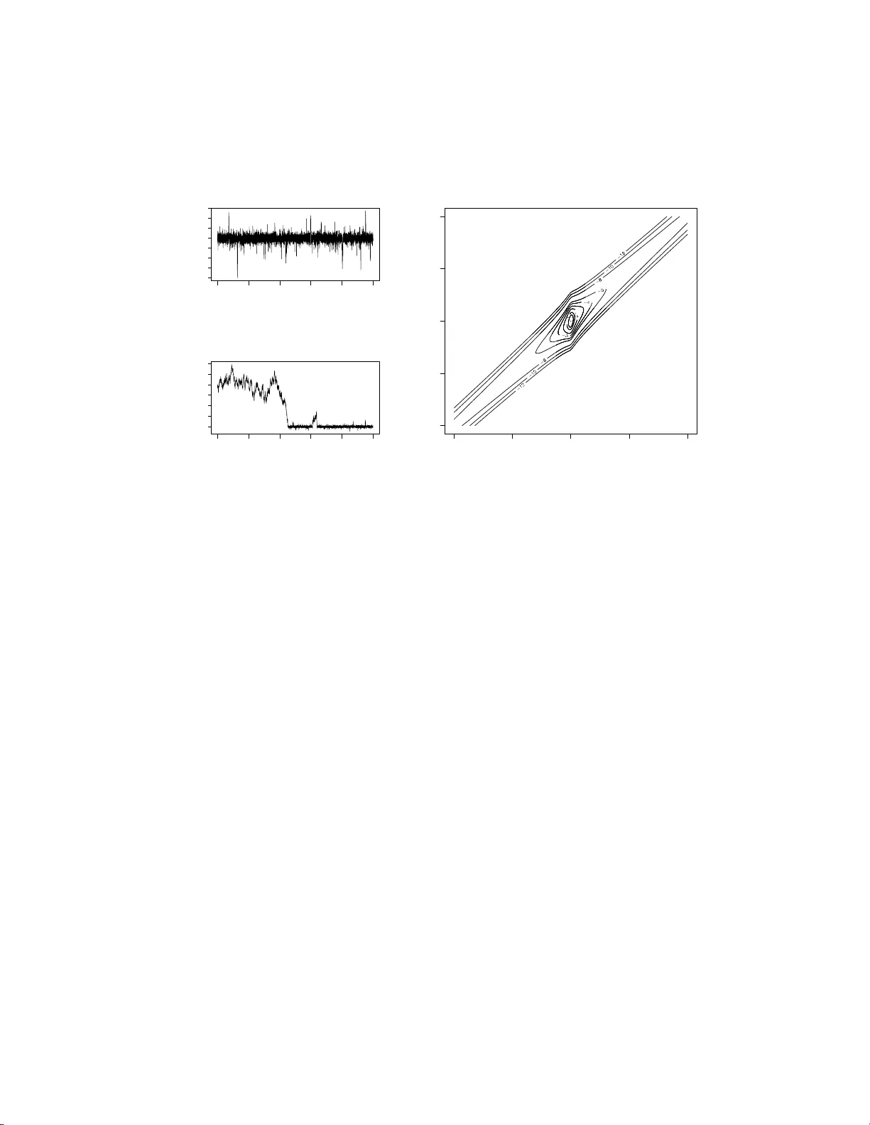
Submitted to the Annals of Statistics ST ABILITY OF THE GI BBS SAMPLER FOR BA YESIAN HIERAR CHICAL MODELS By Omiros P ap aspiliopoul os ∗ and Gare th R ob er ts University of Warwick and L anc aster Univ e rsity W e c h aracterise the conv ergence of th e Gibbs sampler which sam- ples from the joint posterior distribut ion of parameters and missing data in h ierarc hical linear mo dels with arbitrary symmetric error d is- tributions. W e show that the con vergence can be uniform, geometric or sub -geometric dep en ding on the relative tail b ehaviour of t he error distributions, and on th e parametrisation c hosen. Our theory is ap- plied to characterise the converg ence of th e Gibbs sampler on latent Gaussian pro cess mo dels. W e indicate how th e theoretical framew ork w e introduce will b e useful in analyzing more complex mo dels. 1. Introduction. Hierarc hical mo d elling is a widely adopted approac h to constructing complex statistical mo dels. The app eal of the metho d lies in the simp licit y in sp ecifying a highly m ultiv ariate model b y joining many sim- ple and trac table mo dels, the foundational justification b ased on th e ideas o f partial exc hangeabilit y , the flexibilit y to extend or simplify the mo d el in the ligh t of new information, and the ease of inference using p o we rful Mark o v c h ain Monte Carlo (MCMC) metho ds wh ic h ha v e b een dev elop ed to this end dur ing the last tw o decades. Thus, hierarchica l mod els hav e b een used in man y area s of applied statistics such as ge ostatistics [ 8 ], longitudinal anal- ysis [ 9 ], disease mappin g [ 3 ], and financial econometrics [ 23 ] to n ame just a few. ∗ Researc h fund ed by EP SRC gran t GR/S61577/01 AMS 2000 subje ct classific ations: Primary 65C05; secondary 60J27 Keywor ds and phr ases: Geometric ergod icit y , capacitance, collapsed Gibbs sampler, state-space mo dels, parametrisation, Ba yesia n robustness 1 imsart-aos ver. 2007/01/24 file: papaspi liopoulos_rob erts_stabilty-REVISION.tex date: October 30, 2018 2 P AP A SPILIOPOULO S AND ROBER TS A rather general f orm of a t wo -lev el hierarc h ical mo d el is Y ∼ L ( Y | X ) X ∼ L ( X | Θ) , (1) where L ( X ) and L ( Y | X ) denote the distribu tion of X and the conditional distribution of Y g iv en X resp ectiv ely . W e w ill r efer to Y a s th e data, X as the missing d ata and Θ as the p arameters. In a Ba y esian co nte xt the mo del is completed by sp ecifying a prior distribution for Θ. Typically the dimension of X is muc h larger than that of Θ and it can increase w ith the size of the data set. Most of the applications cited ab o v e fit in to ( 1 ) b y imp osing the appropriate structur e on L ( Y | X ) and L ( X | Θ). It is straigh tforward to construct mo d els with more leve ls. Ba ye sian inference for ( 1 ) in volv es the p osterior distribution L ( X, Θ | Y = y ). This is typicall y analytic ally in tractable, b ut it can b e sampled relativ ely easily usin g the Gibbs samp ler [ 29 ], by simulating iterativ ely from the t wo conditional distribu tions L ( X | Θ , Y = y ), and L (Θ | X , Y = y ). It has b een d emonstrated b oth theoretically and empirically that the con vergence (to b e formally defin ed in Section 3 ) of th e Gibb s samp ler r elates to t he structure of the hierarchica l mod el and particularly to the d ep enden ce b et w een th e up dated comp onent s, X and Θ. Nev ertheless, the exact wa y in whic h the mo d el structure inte rferes w ith the con v ergence remains largely unresolv ed. C oncrete theoretical results exist only for Gauss ian hierarc hical mo dels, but we will see that these results do not extend to more general cases. Although in teresting c h aracterizat ions of the conv ergence rate in term s of the dep end ence b et ween X and Θ exist when the Gibb s sampler is geometrically ergo dic [ 1 ], there exist no general results which establish geometric ergo d icit y for the Gibbs sampler. Th e difficu lt y in obtaining suc h general results lies in the in trinsic dep endence of the con v ergence of th e Gibb s sampler on the mo del str ucture. In this pap er we show explicitly h o w the relativ e tail b eha viour of L ( Y | X ) and L ( X | Θ) determines the stabilit y of the Gibbs sampler, i.e. whether imsart-aos ver. 2007/01/24 file: papaspiliopo ulos_roberts _stabilty-REVISION.tex date: October 30, 2018 ST ABILITY OF GIBBS SAMPLER 3 the conv ergence is u n iform, geometric or su b-geometric. Moreo ver, we sho w that the r elativ e tail b eha viour d ictates the typ e of parametrisation that should b e adopted. In order to r etain tractabilit y and formulate inte rpr etable and easy to c h ec k conditions we restrict atten tion to the class of linear hier- arc h ical mo dels with general error d istributions; the precise mo del structur e is giv en in S ection 2.1 . Nev ertheless, our main theoretical r esu lts, in par- ticular Th eorems 3.3 , 3.4 , 3.5 and 6.3 , and the metho dology for proving them are exp ected to b e u seful in a muc h more general cont ext than the one considered h ere. Consideration of the class of linear n on-Gaussian h ierarc h ical m o dels is not merely motiv ated by mathematical con venience. Th ese mo d els are very useful in real applications, for example in longitudinal rand om effects mo d- elling [ 9 , 13 ], time series analysis [ 4 , 12 , 28 ] and sp atial mo delling [ 8 ]. Th ey also are a fun damen tal to ol in the robust Bay esian analysis [ 7 , 20 , 22 , 30 ]. F urtherm ore, we will see that the stabilit y of the Gibbs sampler for linear non-Gaussian mo d els is v ery different compared to the Gaussian case, the lo cal dep en d ence b et we en X and Θ b eing crucial in the n on-Gaussian case. Notice th at seve ral other mo d els can b e approximate ly written as linear non- Gaussian mo d els. Actually , this work has b een motiv ated by the b ehavio ur of MCMC for non-Gaussian Ornstein-Uhlneb ec k s to c h astic v olatilit y mo dels [ 23 ]. The pap er is organised as follo ws. Section 2.1 sp ecifies the mod els we will b e concerned w ith and it establishes some basic notation. Section 2.2 discusses Gibbs sampling under differen t parametrisations of the mo del and Section 2.3 motiv ates the th eory and the metho dology dev elop ed in this pa- p er by a simple example. Section 3 is th e th eoretical core of this pap er; the section commences with a short review of stabilit y concepts for the Gibbs sampler; Section 3.1 recalls the existing results f or Gauss ian linear m o dels; Section 3.2 deve lops stabilit y theory for hierarchica l mo dels and states three main theorems for the stabilit y of the Gibbs sampler; based on these theo- rems Section 3.3 provides the c haracterizatio n of the stabilit y of the Gibbs imsart-aos ver. 2007/01/24 file: papaspiliopo ulos_roberts _stabilty-REVISION.tex date: October 30, 2018 4 P AP A SPILIOPOULO S AND ROBER TS sampler under different parametrisations for a br oad class of linear hierarc hi- cal mo d els; S ection 3.4 considers an alternativ e augmenta tion scheme when one of the error distribu tions is a scale mixture of normals and compares the con vergence of a thr ee-comp onent Gib b s samp ler with that of its collapsed t wo-co mp on ent coun terpart. Section 4 extends the theory to h ierarchical mo dels whic h in v olv e laten t Gaussian p ro cesses. Sectio n 5 d iscu sses exten- sions and con tains some practical guidelines. Section 6 con tains the pro ofs of all theorems and prop ositions. The pro ofs are based on establishing ge- ometric dr ift conditions and minorization conditions and using capacitance argumen ts in conju nction with C heeger’s in equalit y . 2. Mo dels, parametrisations and motiv ation. 2.1. Line ar hier ar chic al mo dels. The mo dels w e consider in this pap er are of the follo wing form , w here Y i is m i × 1, C i is m i × p , X i is p × 1, D is p × 1 and Θ is a scalar: Y i = C i X i + Z 1 i , i = 1 , . . . , m X i = D Θ + Z 2 i . (2) Z 1 i , i = 1 , . . . , m , are iid with distribution L ( Z 1 ), Z 2 i , i = 1 , . . . , m , are iid with distribu tion L ( Z 2 ), and L ( Z 1 ) and L ( Z 2 ) are symm etric d istr ibutions around 0 (a v ector of 0s with the appropriate dim en sion). In the sequel, b old-face letters will corresp ond to v ectors and matrices, capital letters to random v ariables and lo we r-case letters to their realisations. In this setting Y = ( Y 1 , . . . , Y m ) and X = ( X 1 , . . . , X m ). The fi rst equation in ( 2 ) will b e termed the observation e quation and the second th e hidden e qu ation . It is often con ve nientl y assumed that b oth L ( Z 1 ) and L ( Z 2 ) are Gaus- sian. Ho w ev er there are several applications where this assump tion is clearly inappropriate, esp ecially if w e w ish to mak e the inference ab out X robust in the presence of pr ior-d ata conflict. It is kno w n [see e.g. 20 , 22 , 30 , and references therein] that if the tails of L ( Z 1 ) are hea vier than the tails of L ( Z 2 ) then inference for X is r ob u st to outlying observ ations, whereas if imsart-aos ver. 2007/01/24 file: papaspiliopo ulos_roberts _stabilty-REVISION.tex date: October 30, 2018 ST ABILITY OF GIBBS SAMPLER 5 L ( Z 2 ) h as hea v ier tails than L ( Z 1 ) inference for X is less influ enced b y the prior in case of data-prior conflict; these r obustness is absent from Gauss ian mo dels. This t yp e of rob u st mo d elling has b een u ndertak en in time-series analysis, see for example [ 12 ]. 2.2. Gibbs sampling and p ar ametrisation s. A s is common in this frame- w ork, we place an improp er flat prior on Θ, which in this con text leads to a prop er p osterior. Ba y esian inference for ( 2 ) inv olv es th e joint p osterior d is- tribution L ( X , Θ | Y = y ), w hic h w ill abbreviate to L ( X , Θ | Y ). Although it is often analytically in tractable, it can b e sampled easily using the Gibbs sampler. The parametrisation P 0 := ( X , Θ) is termed the c e ntr e d p ar ametrisation . This terminology w as fir s t used in the linear Gaussian con text b y [ 10 ]. F ol- lo win g [ 21 ] we shall use the term more generally to r efer to a parametri- sation where the parameters and th e d ata are conditional ly indep end en t giv en the missing data. W e can us e the Gibb s sampler to collect samples from L ( U , Θ | Y ) where U = h ( X , Θ), for some inv ertible trans formation h , and then transform the dra ws to obtain samples from L ( X , Θ | Y ). In the rest of the pap er we will use P to refer to a general p arametrisation ( U , Θ). It is kno wn [ 16 ] that th e con verge nce (to b e form ally introd uced in Section 3 ) of th e Gibb s sampler impro ves as the dep endence b et ween the u p dated components, U an d Θ, decreases. Hence, the dev elopmen t of general re-parametrisation strategies has b een activ ely r esearc hed, see [ 21 ] for a recen t accoun t. In that w ork, the authors introdu ce the non-c entr e d r ep ar ametr isation P 1 := ( ˜ X , Θ), whic h replaces X with ˜ X := h ( X , Θ), where h is a transformation whic h mak es Θ and ˜ X apriori indep endent. In the con- text of linear hierarchical mo dels ˜ X = ( ˜ X 1 , . . . , ˜ X m ), w here ˜ X i = h ( X i , Θ), and h ( x , θ ) := x − D θ . W e w ill see that P 0 and P 1 present t wo natural c h oices. The prolific expansion in the use o f Gibbs samplin g for inference in hierar- c h ical mo dels durin g the 1990s w as fuelled b y th e app aren t rapid con v ergence imsart-aos ver. 2007/01/24 file: papaspiliopo ulos_roberts _stabilty-REVISION.tex date: October 30, 2018 6 P AP A SPILIOPOULO S AND ROBER TS of the algorithm in many cases. Ho w ev er, to date, there has b een little theo- retical analysis linking the stabilit y of the Gib b s sampler to the s tructure of hierarc hical mo d els. A notable exce ption are th e explicit con verge nce results for Gaussian linear hierarc hical mo dels obtained in [ 24 ] an d summarised in Section 3.1 . The follo wing example is rev ealing as to wh at might go w rong when considering non-Gaussian linear mo dels, and motiv ates the metho dol- ogy and theory dev elop ed in this article. 2.3. A motivating e xample. Consider a simp lifi ed v ersion of ( 1 ) where m = m 1 = C 1 = D = 1, Y = X + Z 1 X = Θ + Z 2 . (3) Assume that L ( Z 1 ) = Ca(0 , 1), a standard Cauc hy d istribution, L ( Z 2 ) = N(0 , 5), and y = 0 is observe d. Figure 2.3 a sho ws the samp led v alues of Θ after t w o in d ep end ent r uns of the Gibbs sampler, eac h of 10 4 iterations. T h e top one is started from the mo de, Θ 0 = 0, and sup erfi cially it app ears to b e mixing well: the auto correlation in the series b ecomes negligible after 10 lags, and most con v ergence diagnostic tests would assess that the chain has con verged. Nev ertheless, the c hain never exits the set ( − 40 , 40), although this is an ev en t w ith stationary probabilit y ab out 0 . 015 . The second run, Figure 2.3 a b ottom, is s tarted fr om Θ 0 = 200, and the c hain sp en ds more than 4,0 00 iterations wo nderin g around Θ 0 . The con tour plot of the join t p osterior log-densit y of X and Θ in Figure 2.3 b, pr o vid es an explanation: the con tours lo ok roughly spherical near the mo de, but they b ecome asymp- totical ly concentrat ed around x = θ as | θ | → ∞ . T h us, restricted to an area around the mo de, X and Θ lo ok roughly indep endent, b ut in the tails they are highly dep endent. In fact, L ( X − θ | Y , Θ = θ ) → N(0 , 5) as | θ | → ∞ , and w e show in S ection 3.3 that the Gibbs sampler wh ic h u p dates X and Θ con verges sub-geometrically . In contrast, L ( ˜ X | Y , Θ = θ ) → L ( ˜ X ), as | θ | → ∞ , and as we show in Section 3.3 th e Gibb s sampler whic h up d ates ˜ X and Θ is uniform ly ergo dic. imsart-aos ver. 2007/01/24 file: papaspiliopo ulos_roberts _stabilty-REVISION.tex date: October 30, 2018 ST ABILITY OF GIBBS SAMPLER 7 0 2000 4000 6000 8000 10000 −40 −20 0 20 iteration θ 0 2000 4000 6000 8000 10000 0 100 200 300 iteration θ X θ −40 −20 0 20 40 −40 −20 0 20 40 (a) (b) Fig 1 . (a): two runs of the Gibbs sampler under P 0 for the mo del ( 3 ) starte d at Θ 0 = 0 (top) and Θ 0 = 200 (b ottom). (b): c ontours of the joint p osterior lo g-density of X and Θ . 3. Conv ergence of the Gibbs sampler for linear hierarc hical mo d- els. Giv en the parametrisation P = ( U , Θ), the tw o-comp onent Gibbs sampler sim ulates iterativ ely from L ( U | Y , Θ = Θ n − 1 ), and L (Θ | Y , U = U n ), wh ere Θ 0 is a starting v alue and n ≥ 1 denotes the iteration n umber. This algorithm generates a Mark o v chain { ( U n , Θ n ) } with stationary d istri- bution L ( U , Θ | Y ). Th e marginal c hain { Θ n } is also Marko v and r ev er s ible with resp ect to L (Θ | Y ) (Lemma 3.1. of [ 16 ]). Moreo v er, it can b e sho wn [ 26 ] that the con vergence rate of the j oin t c hain coincides with th e con v er- gence rate of the marginal c hain, { Θ n } . Notice that this r esult do es not hold for Gibbs samplers wh ic h u p date more than t w o comp onen ts. In the sequel, for an y rand om v ariables W and V , and pr ob ab ility la w µ , we will use the short-hand notation, L ( V | W ∼ µ ) := Z L ( V | W = w ) µ ( dw ) . imsart-aos ver. 2007/01/24 file: papaspiliopo ulos_roberts _stabilty-REVISION.tex date: October 30, 2018 8 P AP A SPILIOPOULO S AND ROBER TS W e will consider the con verge nce of { Θ n } through the total v ariation norm, defin ed as kL h (Θ n | Y , Θ 0 ) − L (Θ | Y ) k = sup | g |≤ 1 | E h { g (Θ n ) | Y , Θ 0 } − E { g (Θ) | Y }| . L h (Θ n | Y , Θ 0 ) is the distribu tion of th e chain after n steps started from Θ 0 , and E h { g (Θ n ) | Y , Θ 0 } is the exp ected v alue of a real b ounded fun ction g with resp ect to this distrib ution. L h (Θ n | Y , Θ 0 ) clearly dep ends on the parametrisation U = h ( X , Θ), sin ce, L h (Θ 1 | Y , Θ 0 ) = L { Θ | Y , U ∼ L ( U | Y , Θ = Θ 0 ) } . Under standard regularit y conditions (Theorem 13.0 .1 of [ 19 ]) the total v ari- ation norm con v erges to 0 as n → ∞ . W e sa y that { Θ n } is ge ometric al ly er go dic wh en th ere exist an r < 1 and some fu nction M ( · ), such that (4) kL h (Θ n | Y , Θ 0 ) − L (Θ | Y ) k ≤ M (Θ 0 ) r n . The smallest r for wh ic h ( 4 ) holds, sa y r h , is kno w n as th e r ate of c onver- genc e of { Θ n } . Ho we v er, the actual distance from s tationarit y will in general dep end on the starting p oin t and this is represented by the term M (Θ 0 ) in ( 4 ). When M ( · ) is b ound ed ab o v e, { Θ n } is called uniformly er go dic . Uni- form ergo dicit y is a v aluable pr op ert y , since it ensures th at the conv ergence of the c hain d o es not d ep end critically on the initial v alue c hosen. Whilst this do es not guarantee rapid con v er gence, it ensu res that the “bu rn-in” problem cannot b ecome arbitrarily bad from certain starting p oin ts. Geometric ergo dicit y is a qu alitativ e stabilit y prop ert y , and geometrically ergo dic algorithms ma y still conv erge slo w ly and giv e Monte Carlo estimates with high v ariance (for example when r h ≈ 1). Ho we v er, algorithms whic h fail to b e geo metrically ergo dic can lead to v arious u ndesirable p rop erties, including the break do wn of the cen tral limit theorem for ergo dic a verag e es- timates. In this case the sim ulation can b e unreliable and the d ra wn samples migh t p o orly represent the target distribution. imsart-aos ver. 2007/01/24 file: papaspiliopo ulos_roberts _stabilty-REVISION.tex date: October 30, 2018 ST ABILITY OF GIBBS SAMPLER 9 T o keep nomenclature simple we will ident ify a parametrisation P = ( U , Θ) with the Gibbs sampler whic h up dates U and Θ. Thus, w e sa y th at a parametrisation P is geometrically (resp ectiv ely u niformly) ergo dic, if th e Gibbs sampler imp lemen ted usin g this parametrisation is geometricall y (r e- sp ectiv ely u niformly) ergo dic. 3.1. Gaussian mo dels. Th e Gibbs sampler for the Gaussian linear mo d el is geometrically ergo d ic with r ate giv en in [ 24 ]. In the simp lified mo del ( 3 ) assume that L ( Z i ) = N (0 , σ 2 i ) , i = 1 , 2, and defi ne κ = σ 2 2 / ( σ 2 2 + σ 2 1 ). Th en, [ 21 ] b uilding on the results of [ 24 ] s ho w ed that, when U = h ( X , Θ ) = X − ρ Θ, (5) r h := r ρ = ( ρ − (1 − κ )) 2 ρ 2 κ + (1 − ρ ) 2 (1 − κ ) = { corr( U, Θ | Y ) } 2 whic h give s rise to the tw o sp ecial cases of interest, r 0 = 1 − κ , r 1 = κ . I n this s etting, the dep end ence b etw een U and Θ is appropr iately quant ified b y the correlat ion coefficient , and ( 5 ) shows that the larger the correlation the worse the con vergence . Man y refinements and generalizations of these results can b e f ound in [ 24 ], [ 21 ] and [ 17 ]. Notic e that b oth P 0 and P 1 are geometrica lly ergo dic. P 0 con verges rapidly when the observ atio n equatio n is “more precise” than th e hidden equation, that is σ 1 << σ 2 , and it con v erges slo wly when the hidden equation is relativ ely p recise. P 1 con verges rapid ly when the hid den equation is r elativ ely more pr ecise. 3.2. Gener al the ory for line ar hier ar chic al mo dels. This s ection giv es general results w hic h can b e us ed to c haracterise the stabilit y of the Gibbs sampler on linear h ierarchical mo dels of the form ( 2 ) wh er e the X i s are univ ariate and D = 1. Our results are v alid when m > 1 and m i > 1 (see Remark 1 in p age 13 ), how ev er in ord er to k eep the notation simple we will w ork with the simp lified mo del ( 3 ), where all Y , X and Θ are scalars. L ( Z 1 ) and L ( Z 2 ) are arbitrary symm etric distr ib utions with con tin uous b ounded ev eryw here p ositiv e densities, f 1 and f 2 resp ectiv ely; common examples in - clude the Gaussian, the Cauc hy and the double exp onent ial. Th is section giv es the general resu lts, while Section 3.3 applies them to charact erise the imsart-aos ver. 2007/01/24 file: papaspiliopo ulos_roberts _stabilty-REVISION.tex date: October 30, 2018 10 P AP A SPILIOPOULO S AND ROBER TS con vergence of th e Gibbs sampler for (a b r oad class of ) linear non-Gaussian hierarc hical mo dels. Section 4 deals with extensions wh ere the X i s are v ec- tors of dep end en t v ariables, therefore cov ering state-space and spatial m o d- els. Nev ertheless, the results ev en for the more structured mod els follo w relativ ely easily from the results of this section. All pro ofs are deferred to Section 6 . W e b egin by int ro d u cing a collectio n of p osterior robustness concepts, whic h are related with the b eha v iour of the conditional p osterior distri- bution L ( U | Y , Θ = θ ) as | θ | → ∞ . All these concepts ha ve statistical in terpretations b ut they turn out to p r o vid e the required mathematical con- ditions for charac terising the stabilit y of the Gibb s sampler, as w e s ho w in Theorems 3.3 , 3.4 and 3.5 b elow. Definition 3.1 . The p ar ametrisatio n P = ( U, Θ) i s c al le d: 1. p artial ly tight in p ar ameter (PTIP), if for al l y , ther e is some k > 0 such that, (6) lim su p | θ |→∞ P ( | U | > k | Y = y , Θ = θ ) < 1 , 2. ge ometric al ly tight i n p ar ameter (GTIP), if ther e exist p ositive c on- stants, a , b (indep endent of θ ) such that for al l θ , P ( | U | > x | Y = y , Θ = θ ) ≤ ae − bx . GTIP not only implies that L ( U | Y , Θ = θ ) is a tigh t family of distri- butions, b ut also that th e tail p robabilities are b ound ed exp onent ially . (W e recall that a family of distribu tions on the real line, sa y F θ , indexed b y a scalar θ , is called tight wh en lim k →∞ sup θ F θ ([ − k , k ] c ) = 0.) Clearly , GTIP is muc h stronger cond ition than PTIP . W e consider also th e follo wing mo del robustness concepts. Definition 3.2 . We say that the line ar hier ar chic al mo del ( 3 ) is imsart-aos ver. 2007/01/24 file: papaspiliopo ulos_roberts _stabilty-REVISION.tex date: October 30, 2018 ST ABILITY OF GIBBS SAMPLER 11 1. r obust in p ar ameter (RIP), i f lim | θ |→∞ L ( X | Y = y , Θ = θ ) = L ( Z 1 + y ) , 2. r obust in data (RID), if lim | θ |→∞ L ( ˜ X | Y = y , Θ = θ ) = L ( ˜ X ) , 3. data uniformly r elevant (DUR), if ther e e xist p ositive c onstants d , k such that for al l | θ | > k , | E { X | Y = y , Θ = θ }| ≤ | θ | − d, 4. p ar ameter u ni f ormly r elevant (PU R), if ther e exist p ositive c onstants d , k such that for al l | θ | > k , sgn ( θ ) E { X − y | Y = y , Θ = θ } ≥ d. These defin itions c h aracterise the h ierarc h ical mo del acc ording to ho w inference for X (conditionally on Θ = θ ) is affec ted b y a large discrepancy b et w een th e data y and the prior gu ess θ . When the mo del is RIP inference for X ignores θ , and it is symmetric around y . C on v ersely , when the mo del is RID inference for X ignores th e data and b ecomes symmetric around θ . When the mo del is DUR (PUR) the d ata (the parameter) alw a ys influences the conditional exp ectatio n of X . Notice that wh en the mo d el is RIP P 0 is PTIP (although not n ecessarily GTIP), and w h en it is RI D P 1 is PTIP . The example in Section 2.3 describ es a RI D mo del. A mo d el can b e b oth DUR and PUR (for example the Gaussian linear mo d el). Theorem 3.3 . Consider the line ar hier ar chic al mo del ( 3 ) wher e the er- r or densities f 1 and f 2 ar e c ontinuous, b ounde d and everywher e p ositive. If P 0 ( P 1 ) is P TIP, then it is uniformly er go dic. Theorem 3.4 . Consider the line ar hier ar chic al mo del ( 3 ) wher e the er- r or densities f 1 and f 2 ar e c ontinuous, b ounde d and everywher e p ositive. If the mo del is RID then P 0 is not ge ometric al ly er go dic, and if the mo del is RIP then P 1 is not ge ometric al ly er go dic. imsart-aos ver. 2007/01/24 file: papaspiliopo ulos_roberts _stabilty-REVISION.tex date: October 30, 2018 12 P AP A SPILIOPOULO S AND ROBER TS Distribution Code Densit y g ( x ) up to prop ortionality Cauc hy C σ 2 / (1 + x 2 ) Double exp onential E exp {−| x | /σ } Gaussian G exp  − ( x/σ ) 2 / 2  Exp onential pow er distribution L exp  −| x/σ | β  , β > 2 T a ble 1 Distributions for the err or terms and their densities. In the p ap er they ar e c o de d ac c or di ng to the letter in the midd le c olumn. The pr o of Theorem 3.4 is based on the general Theorem 6 .3 ab out Marko v c h ains on the real line, w hic h is stated and p ro v ed in S ection 6 . Theorem 3.5 . 1. If the mo del is DUR, P 1 is GTIP , and L ( Z 2 ) has finite moment gene r ating function in a neighb ourho o d of 0 , then P 0 is ge o- metric al ly er go dic. 2. If the mo del is PUR, P 0 is GTIP , and L ( Z 1 ) has finite moment gene r ating function in a neighb ourho o d of 0 , then P 1 is ge ometri- c al ly e r go dic. The theorems are prov ed by establishing a geometric d r ift cond ition. The requirement s of GTIP for P 1 ( P 0 ) and finite momen t generating function for L ( Z 2 ) ( L ( Z 1 )) are in order to tilt exp onent ially the linear d r ift condition pro vided by DUR (PUR). 3.3. Char acterising the stability of the Gib b s sampler ac c or ding to the dis- tribution tails of the err or terms. In this section, building up on the general theory of Section 3.2 , we c haracterise th e stabilit y of the Gibb s sampler on the linear hierarc hical mo del ( 3 ) for differen t sp ecifications of L ( Z 1 ) , L ( Z 2 ). Although we consider the error d istributions in T able 1 , our pro ofs remain v alid for muc h b r oader families of distribu tions (see Remark 2 on page 13 ). Notice that the exp onential p o wer distribu tion conta ins b oth the Gaussian ( β = 2) and the doub le exp onential ( β = 1) as sp ecial cases. Here we con- sider densities w ith tai ls ligh ter than Gaussian ( β > 2). F or the use of this distribution in Bay esian robus tness see [ 5 ]. W e sh all sp ecify linear mod els giving first L ( Z 1 ) and then L ( Z 2 ), for instance the ( C , E ) mo del corresp onds to ( 3 ) with Cauc hy distribution for imsart-aos ver. 2007/01/24 file: papaspiliopo ulos_roberts _stabilty-REVISION.tex date: October 30, 2018 ST ABILITY OF GIBBS SAMPLER 13 Stability of P 0 L ( Z 1 ) C E G L C U U U U L ( Z 2 ) E N G/U U U G N G G G L N G G G Stability of P 1 L ( Z 1 ) C E G L C U N N N L ( Z 2 ) E U U/G G G G U U G G L U U G G T a ble 2 Stability P 0 (left) and P 1 (right) f or the l ine ar hier ar chic al m o del ( 3 ) for sp e cific ations of the di stribution of the err or terms as in T able 1 . Z 1 , and double exp onential distribu tion for Z 2 . F or eac h mo del we ha ve t wo parametrisations, th us t wo algorithms, P 0 and P 1 . When we refer to the stabilit y of an algorithm we shall write U, G, and N to refer to uniform, geometric and non-geometric (i.e. sub -geometric) ergo d icit y , resp ectiv ely . Theorem 3.6 . The stability P 0 and P 1 is given in T able 2 . R emark 1. The determin in g factor in classifying the stabilit y of a parametri- sation is the tail b eha v iour of L ( Z 1 ) and L ( Z 2 ). Thus, Th eorem 3.6 gener- alises to the case of multiple rand om effects and ob s erv ations: Y ij = X i + Z 1 ij , j = 1 , . . . , m i X i = Θ + Z 2 i , i = 1 , . . . , m where Z 1 ·· and Z 2 · are ind ep endently d istributed identi cally to L ( Z 1 ) and L ( Z 2 ) resp ectiv ely . T his extension is immediate where obvious sufficient statistics exist (the C and N cases). Ho w ev er, s in ce p ro ving formally the full generalisation would b e extremely tedious (although in the same lines as in Section 6 ), we do n ot attempt it h ere. R emark 2. T he same results can b e obtained when any of th e distribu tions considered in T able 2 is replaced b y another symm etric distribution with the same tail b eha viour, wh ich p ossess a b ounded con tin uous ev eryw h ere p ositiv e densit y . imsart-aos ver. 2007/01/24 file: papaspiliopo ulos_roberts _stabilty-REVISION.tex date: October 30, 2018 14 P AP A SPILIOPOULO S AND ROBER TS R emark 3. Different r esults hold when a prop er pr ior f or Θ is imp osed. In this case the con v ergence impr o ves. R emark 4. Th e results of Theorem 3.6 are indep endent of the actual v alue of y . This do es not necessarily h old in other con texts. R emark 5. In the ( E , E ) mo del, the stabilit y dep en d s on the ratio of the scale p arameters in L ( Z 1 ) and L ( Z 2 ). Dep ending on this ratio conv ergence can b e either geometric or u n iform (see Section 6 for details). R emark 6. T he follo wing heuristic can b e d eriv ed fr om T able 2 : con verge nce of P 0 is b est when L ( Z 1 ) has lighter tails than L ( Z 2 ), and worst when it h as hea vier tails. T he situation for P 1 is the rev erse. Both algorithms b ecome more stable the ligh ter the tails of L ( Z 1 ) and L ( Z 2 ) b ecome. 3.4. Conver genc e of the gr oup e d Gibbs sampler. An alternativ e augmen- tation scheme and sampling algorithm can b e adopted when one of the error distributions, sa y L ( Z 2 ) for con v enience, is Gaussian and the other, sa y L ( Z 1 ), is a scale mixture of Gaussian distributions. S ev eral symm et- ric distr ibutions b elong in this class, for in stance the Stu den t-t (th us the Cauc h y) and the doub le exp onen tial [ 2 ]. In this case, Z 1 can b e represente d as Z 1 = V /Q , where V has a standard Gaussian distribu tion and Q is p ositiv e and indep end en t of V . W e can treat Q as missing data and con- struct a thr e e-c omp onent Gibbs sampler whic h up d ates iterat iv ely X , Q and Θ from their conditional distribu tions. (When X = ( X 1 , . . . , X m ) th en Q = ( Q 1 , . . . , Q m ) wh ere Q i is indep endent from Q j for ev ery i 6 = j ). A ma jor computational adv an tage of this app roac h is that L ( X | Y , Θ , Q ) is Gaussian and it can b e easily samp led. Notice th at Q and Θ are indep en - den t giv en X , th u s w e can implemen t the Gibbs sampler using a gr oup e d sc h eme [ 15 ] where Θ and Q are u p d ated in one blo ck. It is of interest to kno w whether the conv ergence of this group ed Gibbs sampler is b etter than the conv ergence of the c ol lapse d Gibbs samp ler (as d efined in [ 15 ]), wh ere Q has b een integ rated out. T he “Three-sc hemes Theorem” of [ 15 ] states that imsart-aos ver. 2007/01/24 file: papaspiliopo ulos_roberts _stabilty-REVISION.tex date: October 30, 2018 ST ABILITY OF GIBBS SAMPLER 15 the norm of the transition op erator of the group ed Gibbs sampler is larger than the one which corresp onds to the collapsed Gibbs sampler. This result, ho w ev er, is not enough to guaran tee that the collapsed sampler will h av e b etter conv ergence rate. In ord er to giv e a concrete answer, we consider the imp ortan t sp ecial case, where L ( Z 1 ) is the Cauch y distribu tion, therefore Q ∼ Ga(1 / 2 , 1 / 2). W e ha v e the follo wing prop osition, w hose pro of is b ased on Th eorem 6.3 . Pr opos ition 3.7 . The gr oup e d Gibbs samp ler is not ge ometric al ly er- go dic. This r esu lt remains true for a num b er of random effects m > 1, and it will hold for more general Student -t distributions. Th is r esult has imp ortant practical imp lications esp ecially in algo rithms for late nt Gaussian mo d els, considered in Section 4 . It is also significant that it cont rasts the result ob- tained by [ 27 ], who establishes geometric ergo dicity for v ariance comp onen t mo dels (of which the mo del considered here is a sp ecial case). How ev er, the result in [ 27 ] is tru e when the num b er of data Y ij , m i , p er random effect X i is larger than some num b er bigger than one, whereas in Lemma 3.7 w e tak e m i = 1. 4. Latent Gaussian pro cess mo dels. In this section w e consider a rather sp ecific though useful mo d el and demonstrate that th e results of Section 3.2 can b e extended quite readily to this con text giving some clear- cut conclusions an d advice for practical im p lemen tation. T he resu lts b elo w are certainly not the most general p ossible, but it is hop ed that th e metho d of pro of will indicate h o w an alogous mo dels might b e addr essed . Theorem 4.1 . Consider the latent Gaussian pr o c ess mo del: Y = X + Z 1 X = 1 Θ + Σ 1 / 2 Z 2 imsart-aos ver. 2007/01/24 file: papaspiliopo ulos_roberts _stabilty-REVISION.tex date: October 30, 2018 16 P AP A SPILIOPOULO S AND ROBER TS wher e Z 1 = { Z 11 , . . . Z 1 p } is a ve ctor of indep endent and identic al ly dis- tribute d standar d Cauchy r andom variables, Z 2 = { Z 21 , . . . Z 2 p } is a ve c tor of indep endent and identic al ly distribute d standar d Gaussian r andom vari- ables, and 1 is a ve ctor of 1 ’s. Σ is assume d known and a flat is prior is assigne d to Θ . Then 1. P 0 fails to b e ge ometric al ly er go dic; 2. P 1 is uniformly er go dic. As we remark ed on page 13 , the result holds w hen the C auc hy is gener- alised to a Stud en t-t with an y degrees of fr eedom. The MCMC for late nt Gaussian p ro cess mo dels is often imp lemented using a d ifferen t augmen- tation sc heme. As in Section 3.4 , we can augmen t the mo del with Q = ( Q 1 , . . . , Q p ), where L ( Q i ) = Ga(1 / 2 , 1 / 2). Ho we v er, a s im ilar argument as in the pr o of of Pr op osition 3.7 sh o w s that th e Gibb s sampler which up dates X , Q and Θ is not geometricall y ergod ic. As a n umerical illustration we consider a linear non-Gaussian state-space mo del: X 1 , . . . , X p are consecutive d ra w s from an AR(1) mod el, whic h are observ ed with Cauc hy error. W e ha ve sim ulated p = 100 data from th is mo del using Θ = 0. Th e up d ate of Θ g iv en X is from a Ga ussian distrib ution, ho w ev er the up date of X giv en Θ and Y is non-trivial. W e u p date all th e states tog ether using a highly efficient Langevin al gorithm, see [ 6 ] for details. Moreo ve r, we p erform sev eral up dates of X for every up date of Θ so that our results are not critically affected by not b eing able to simulate d ir ectly f rom L ( X | Y , Θ ). Figure 4 depicts our theoretical findings. P 0 has a rand om w alk-lik e b eh a viour in the tails, wh ereas P 1 returns rapidly to the mo dal area. O n the other hand , P 0 mixes b etter than P 1 around the m o de. Note that the instabilit y of P 0 in the tails is not due to lac k of information ab out Θ but du e to the robustn ess prop erties of th e m o del. In th is cont ext it is defin itely advisable to mix b etw een P 0 and P 1 , i.e to use a h ybrid sampler whic h at ev ery iteration with some pr ob ab ility up dates (Θ , X ) and with the remaining p robabilit y it u p d ates (Θ , ˜ X ). This hybrid sampler will in herit the uniform ergo dicity from P 1 but it will also mix we ll imsart-aos ver. 2007/01/24 file: papaspiliopo ulos_roberts _stabilty-REVISION.tex date: October 30, 2018 ST ABILITY OF GIBBS SAMPLER 17 0 20 40 60 80 100 −1.0 −0.5 0.0 0.5 1.0 1.5 iteration 0 20 40 60 80 100 −0.5 0.0 0.5 1.0 iteration 0 20 40 60 80 100 0 100 200 300 400 500 iteration 0 20 40 60 80 100 0 100 200 300 400 500 iteration Fig 2 . Two runs of P 0 (left) and P 1 (right) with two differ ent starting values: Θ 0 = 0 (top) and Θ 0 = 500 (b ottom). around the mo d al area. 5. Discussion. W e h a ve obtained rigorous theoretical r esults for th e stabilit y of the Gibbs sampler wh ic h explores the p osterior distribu tion aris- ing from a broad class of linear hierarc hical mo dels. W e ha v e also pro v ed results regarding more complicate d hierarchica l m o dels with laten t Gaus- sian pro cesses, an d we ha ve compared different sampling schemes. W e ha v e sho wn ho w the mo del structure dictates whic h parametrisatio n should b e adopted for imp ro ving the conv ergence of the Gibbs sampler. Our results are certainly not the most general p ossible, th ou gh the metho d of pro of we hav e used indicates clearly ho w analogous problems might b e addressed. As an example of this, it is easy to extend th e conclusions of T able 2 to the case wher e the light-t ailed distrib utions are replaced by (say) uniform distr ib utions on fin ite ranges. The rob u stness concepts of PT IP , GTIP , RIP and RID are already stated in a general form, while the con- cepts of DUR and PUR can b e translated in a natural wa y usin g L yapuno v imsart-aos ver. 2007/01/24 file: papaspiliopo ulos_roberts _stabilty-REVISION.tex date: October 30, 2018 18 P AP A SPILIOPOULO S AND ROBER TS drift cond itions. F amil ies of mo d els to whic h w e are cur ren tly inv estigating extensions of ou r metho ds, in clud e sto c hastic vola tilit y mo dels pr ev alent in finance. Th is is the sub ject of on -going researc h by the auth ors. The ge neral heuristic is clear - the stabilit y of the cen tred and non-cen tred algorithms, P 0 and P 1 resp ectiv ely , dep ends on the relativ e tail b eha viour of L ( Z 1 ) and L ( Z 2 ), with the centred metho d b eing more stable when L ( Z 1 ) is relativ ely light tailed, and the non-cente red b eing m ore stable w hen L ( Z 2 ) is relativ ely light taile d. An additional conclusion of T able 2 is that, as exp ected, b oth algorithms p ossess comparativ ely more stable con vergence prop erties the ligh ter the tails of L ( Z 1 ) and L ( Z 2 ) b ecome. The main m essage of the p ap er for the MCMC pr actitioner is a p ositiv e one: the comp etition b et ween P 0 and P 1 w orks to the user’s b enefit. O ur results suggest that a com bination of P 0 and P 1 is often desirable. When the tails of the error distribu tions are very different w e h a ve found that one of the algorithms might b e very go o d for visiting the tails of the target distribution wh ereas the other for exploring the mo dal area (as for example w e demonstrate in Fig ure 4 ). Therefore, it is advisable to us e a h yb rid Gibbs sampler w h ic h at ev ery iteration w ith some pr obabilit y up dates (Θ , X ) an d with the remaining p robabilit y it u p dates (Θ , ˜ X ). Moreov er, by lin k in g the stabilit y of th e Gibbs sampler to th e robustness prop erties of the hierarc h ical mo del we pro vide intuition whic h can b e foun d us eful for mo dels outside the scop e of this pap er. Another interesting pr o duct of this wo rk is th at linear re-parametrisations, whic h can sub stan tially impro v e th e conv ergence rate in (app ro ximately) Gaussian mo d els, m igh t b e of little relev ance when the tail b eha viour of L ( Z 1 ) is very differen t f r om L ( Z 2 ). F or example, in (C,G) mo del, where the observ ation error is Cauch y and th e prior f or X is Gaussian, we can pro v e that the Gibbs samp ler wh ic h up dates U = X − ρ Θ and Θ is sub- geometrica lly ergo d ic for all ρ < 1, whereas it is uniformly ergo dic for ρ = 1 as we already kno w fr om Theorem 3.6 . This emphasizes the sp ecial role of P 1 , whic h d iffers b ecause of the prior indep endence it induces on ˜ X and Θ. imsart-aos ver. 2007/01/24 file: papaspiliopo ulos_roberts _stabilty-REVISION.tex date: October 30, 2018 ST ABILITY OF GIBBS SAMPLER 19 This r esu lt suggests that conditional augmen tation (as in [ 18 ]) algorithms migh t fail to b e geometrically ergo dic wh en P 0 do es. All the results present ed h ere are s p ecific to the Gibbs s ampler, how ev er our find ings are clearly relev ant to conte xts w here certain direct simulat ion steps hav e to b e replaced by appr opriate Metrop olis-Hastings steps (as f or example in the sim ulation illustration in Section 4 ). It is w orth men tioning that once we ha ve established geomet ric ergod icit y for an algo rithm, it is imp ortan t to obtain computable b ounds on th e rate of con v ergence. W e ha ve not attempted to do s o, since it is outside the fo cus of this pap er. F or adv ances in this direction see for examp le [ 11 , 27 ]. One in teresting feature resulting from this pap er is that the marginal c h ain { Θ n } of the Gibbs sampler on linear non-Gaussian mo dels often b e- ha v es asymptotical ly (i.e in the tails) lik e a r andom auto-regressio n of the form: Θ n = ρ n Θ n − 1 + ǫ n where ρ n is a rand om v ariable taking v alues in [0 , 1], and ǫ n is an err or term. F or instance in the (G, G) case of Theorem 3.6 for P 0 ( P 1 ) ρ n is deterministically equal to r 0 ( r 1 ) defined in S ection 3.1 . Th e cases where w e demonstrate that the algorithm is rand om-w alk lik e corresp ond to taking ρ n = 1 ( almost sur ely ). F urth er m ore in a n umb er of cases, ρ n is gen uin ely random. F or ins tance, in the (E, E) case with iden tical rates, ρ n ∼ U [0 , 1]. In th e (C,C) case, w e fin d that ρ n tak es the v alue 0 or 1 with probabilities determined by th e s cale parameters of th e Cauc hy distribu tions inv olve d. An extension of our ideas is p ossible for h ierarchical mo dels with more lev els. F or in stance consider the linear structure giv en by Y = Θ 1 + Z 1 Θ i = Θ i +1 + Z i +1 , i = 1 , . . . d − 1 , (7) with a flat prior on Θ d . S ince Y is the only information av ail able, the p oste- rior tails of Θ 1 , Θ 2 . . . b ecome progressiv ely heavi er. If at an y stage, Z i has ligh ter tails than Z i − 1 , then whenever Θ i − 1 and Θ i +1 strongly disagree, the imsart-aos ver. 2007/01/24 file: papaspiliopo ulos_roberts _stabilty-REVISION.tex date: October 30, 2018 20 P AP A SPILIOPOULO S AND ROBER TS conditional distribu tion of Θ i giv en Y , Θ − i will virtually ignore Θ i − 1 and hence the data. Th is will lead to p oten tial instabilities in the c h ain in com- p onents Θ i , Θ i +1 , . . . , Θ d . W e call this phen omenon th e quick sand pr inciple, and this is the sub ject of ongoing inv estigation by the authors. 6. Pro ofs of main results. In the sequel we will use π to denote the densit y of any stationary measure, in particular π ( θ | y ) and π ( x | y , θ ) will b e the L eb esgue dens ities of L (Θ | Y = y ) and L ( X | Y = y , Θ = θ ) resp ectiv ely . With p ( · , · ) w e denote the transition densit y of a Mark o v c hain, and with Θ 0 and Θ 1 the consecutiv e v alues of the marginal c hain { Θ n } . proof of Theo rem 3.3 . W e show the result for P 0 , since the corre- sp ond ing r esult for P 1 can b e pr o ved in an analogous w a y . In particular, we sho w that when P 0 is PTIP , the transition densit y of the th e marginal c hain { Θ n } , is su c h that inf θ 0 p ( θ 0 , θ 1 ) > 0, and p is also con tin u ous in θ 1 . This guaran tees un iform ergo d icit y by Th eorem 16.0.2 of [ 19 ]. p ( θ 0 , θ 1 ) = Z f 2 ( | x − θ 1 | ) π ( x | y , θ 0 ) dx ≥ Z k − k f 2 ( | x − θ 1 | ) π ( x | y , θ 0 ) dx ≥ inf | x |≤ k f 2 ( | x − θ 1 | ) P ( | X | ≤ k | Y = y , Θ = θ 0 ) , for k suc h that ( 6 ) holds. Since f 1 and f 2 are everywhere p ositiv e, b ound ed and con tinuous, P ( | X | ≤ k | Y = y , Θ = θ 0 ) is also p ositiv e and con tinuous in θ 0 , therefore b y the PTIP prop ert y it follo ws that inf θ 0 P ( | X | ≤ k | Y = y , Θ = θ 0 ) > 0. Moreo v er, inf | x |≤ k f 2 ( | x − θ 1 | ), is p ositiv e and conti nuous in θ 1 , thus the result follo w s . ⊓ ⊔ The pr o of of Theorem 3.4 requires T heorem 6.3 , hence it is pr o ved on page 24 . The p ro of of Theorem 3.5 r equ ires the follo wing lemmas. Lemma 6.1 . 1. If ( 3 ) is DU R and the p ar ametrisation ( ˜ X , Θ ) is GTIP, then for al l suffici ently smal l α > 0 , E n e αX | Y , Θ = θ o ≤ e αθ (1 − αd/ 2) , for θ > k E n e − αX | Y , Θ = θ o ≤ e − αθ (1 − αd/ 2) , for θ < − k , wher e k , d ar e define d in Definition 3.2 . imsart-aos ver. 2007/01/24 file: papaspiliopo ulos_roberts _stabilty-REVISION.tex date: October 30, 2018 ST ABILITY OF GIBBS SAMPLER 21 2. If ( 3 ) is PU R and the p ar am etrisation ( X , Θ ) is GTIP, then for al l sufficiently smal l α > 0 , E n e α ( y − ˜ X ) | Y = y , Θ = θ o ≤ e αθ (1 − αd/ 2) , for θ > k E n e − α ( y − ˜ X ) | Y = y , Θ = θ o ≤ e − αθ (1 − αd/ 2) , for θ < − k , Pr oof. 1. W e will p ro v e only the first inequalit y , for θ > k , since the other is prov ed in a similar fashion. W e define G θ ( t ) = E n e t ( X − θ ) | Y , Θ = θ o , whic h is fin ite for all sufficient ly small t > 0, sa y 0 < t < t 0 for s ome t 0 , and for all θ , since b y the GTIP assump tion L ( | X − θ | | Y , Θ = θ ) has exp o- nen tial or ligh ter tails. By a second ord er T a ylor series exp an s ion of G θ ( t ) around t = 0, w e obtain for some 0 < t 1 < t 0 , and for θ > k , G θ ( t ) = 1 + t E { X − θ | Y , Θ = θ } + t 2 2 E n ( X − θ ) 2 e t 1 ( X − θ ) | Y , Θ = θ o ≤ 1 − td + t 2 2 E n ( X − θ ) 2 e t 1 ( X − θ ) | Y , Θ = θ o . No w p ick α < t 1 small enough so that for all θ > k α E n ( X − θ ) 2 e t 1 ( X − θ ) | Y , Θ = θ o < d . Su c h α exists d u e to the GTIP assu mption. Th en , G θ ( α ) ≤ 1 − αd/ 2 , and the result follo ws. 2. It is prov ed as 1, r ecognising that ˜ X = X − θ . ⊓ ⊔ Lemma 6.2 . 1. If ( 3 ) is DU R and the p ar ametrisation ( ˜ X , Θ ) is GTIP, then for al l suffici ently smal l α > 0 , E n e α | X | | Y , Θ = θ o ≤ e α | θ | (1 − αd/ 2) + K , for | θ | > k , wher e k , d ar e define d in Definition 3.2 , and 0 < K < ∞ . 2. If ( 3 ) is PU R and the p ar am etrisation ( X , Θ ) is GTIP, then for al l sufficiently smal l α > 0 , E n e α | y − ˜ X | | Y = y , Θ = θ o ≤ e α | θ | (1 − αd/ 2) + K , for | θ | > k , wher e k , d ar e define d in Definition 3.2 , and 0 < K < ∞ . imsart-aos ver. 2007/01/24 file: papaspiliopo ulos_roberts _stabilty-REVISION.tex date: October 30, 2018 22 P AP A SPILIOPOULO S AND ROBER TS Pr oof. 1. W e prov e th e result for θ > 0 exploiting the fi rst inequalit y giv en in Lemma 6.1 . The case θ < 0 is p ro v ed analogously but exploiting the second inequalit y of Lemm a 6.1 . Notice that E n e α | X | | Y , Θ = θ o ≤ E n e αX | Y , Θ = θ o + Z 0 −∞ e − αx π ( x | y , θ ) dx, th us, due to Lemma 6.1 w e only need to sho w that the second term of the sum ab o ve can b e b ound ed ab o ve for all θ . R ecall a, b from the GTIP Definition 3.2 . Cho ose α < b . Using in tegration b y parts, w e fin d that th e second summand is b oun ded ab o v e by , e − bθ [ a + α/ ( b − α )], which can ea sily b e b ound ed ab o ve for all θ > k . 2. It is p ro v ed as 1, r ecognising that ˜ X = X − Θ . ⊓ ⊔ proof of Theorem 3.5 1. W e prov e the resu lt establishing a geometric drift condition for the marginal c hain { Θ n } , usin g the function V ( θ ) = e α | θ | , for appropriately c h osen α > 0. Notice fi rst that L (Θ | Y , X = x ) ≡ L (Θ | X = x ) is symm etric around x and has a fi nite momen t generating fu nction in a neigh b our ho o d of the origin. Thus, w orking as in Lemma 6.1 an d Lemma 6.2 , w e can sho w that for all sufficien tly small α > 0, there exists K 1 > 0 and ǫ > 0, su c h that, E { e α | Θ | | X = x } ≤  1 + α 2 ǫ  e α | x | + K 1 . Then, for | θ 0 | > k , and appropriate K 1 > 0 , K > 0, E { e α | Θ 1 | | Y , Θ 0 = θ 0 } = E { E { e α | Θ 1 | | X 1 } | Y , Θ 0 = θ 0 } ≤ E { (1 + α 2 ǫ ) e α | X 1 | + K 1 | Y , Θ 0 = θ 0 } ≤ (1 + α 2 ǫ )(1 − αd/ 2) e α | θ 0 | + K ≤ (1 − αδ ) e α | θ 0 | + K . No w since sta ndard argumen ts (see for exa mple [ 25 ]) sho w that compact sets are sm all for this problem, the Gibbs sampler is s h o w n to b e geometrically ergo dic by Theorem 15.0.1 of [ 19 ]. 2. Th e s econd result is pr o ved almost identica lly . Notice th at L (Θ | Y = y , ˜ X = x ) is sym metric around y − x and p ossesses finite moment ge nerating imsart-aos ver. 2007/01/24 file: papaspiliopo ulos_roberts _stabilty-REVISION.tex date: October 30, 2018 ST ABILITY OF GIBBS SAMPLER 23 function in a neighbou r ho o d of 0, th us as we sho w ed a b ov e, f or all sufficien tly small α > 0, there exists a K 1 > 0 such that, E { e α | Θ | | Y = y , ˜ X = x } ≤  1 + α 2 ǫ  e α | y − x | + K 1 . Using Lemma 6.2 and arguin g as in 1 p ro v es the theorem. ⊓ ⊔ Before pro v in g Th eorems 3.4 and 3.6 we need the follo wing general result ab out Mark o v c h ains on the real line. Theorem 6.3 . L et { W n } b e an er go dic and r eve rsible with r esp e ct to a density π , Markov chain on R with tr ansition density p ( x, y ) which is r andom walk-like in the tails, in the sense that ther e is a c ontinuous p ositive symmetric density q such that (8) lim | x |→∞ p ( x, x + z ) = q ( z ) , z ∈ R . Then 1. π has he avy tails, in the sense tha t (9) lim x →∞ log R ∞ x π ( u ) du x = lim x →∞ log R − x −∞ π ( u ) du − x = 0 ; 2. { W n } is not g e ometric al ly er go dic. proof 1. W e will prov e the result f or x → ∞ , since the case x → −∞ , is pro v ed in th e same wa y . Fix z , δ ∈ R + , and let W denote a rand om v ariable whic h has densit y π . By ( 8 ), there exists k > 0 suc h that for x > k p ( x + z , x ) p ( x, x + z ) ≤ (1 + δ ) . This uses the f act that q ( z ) > 0. Thus by reversibilit y , and for x > k , π ( x ) π ( x + z ) = p ( x + z , x ) p ( x, x + z ) ≤ (1 + δ ) , so that (10) π ( x + z ) ≥ (1 + δ ) − 1 π ( x ) . imsart-aos ver. 2007/01/24 file: papaspiliopo ulos_roberts _stabilty-REVISION.tex date: October 30, 2018 24 P AP A SPILIOPOULO S AND ROBER TS In tegrating ( 10 ) o v er x > k , giv es that (11) P ( W > k + z ) ≥ (1 + δ ) − 1 P ( W > k ) . Iterating this expr ession, and after some algebra, we get th at lim n →∞ log P ( W > k + nz ) n ≥ − δ, whic h, sin ce δ can b e c h osen arbitrarily small, prov es the statemen t. 2. The second follo w s fr om the follo wing standard capacitance argum en t; see [ 25 ] f or s imilar argum ents for MCMC algorithms and [ 14 ] f or an intro- duction to Cheeger’s inequalit y using capacitance. Cheeger’s inequalit y for rev ersible Mark ov chains imp lies that geometric ergod icity must fail if w e can find k > 0, suc h that th e probability P  | W 1 | ≤ k | W 0 ∼ π ( − k, k ) c  is arbitrarily sm all, where w e use π ( − k, k ) c to denote the dens it y π restricted and re-normalised to the set {| x | > k } . Notice that ( 11 ) imp lies that for sufficien tly large k , for | x | > k , and an y l > 0, there P ( | W 1 | > x + l | W 0 > k ) ≥ (1 + δ ) − 1 ≥ 1 − δ . No w c ho ose l sufficient ly large that R ∞ l q ( u ) du < δ then for all | x | > k , P ( | W 1 | < k ) ≤ P ( | W 1 | < k | W 0 ∼ π ( − k, k ) c ) + P ( | W 1 − W 0 | > l ) whic h con v erges as | x | → ∞ to a limit b ounded by 3 δ . S ince δ is arbitrary , the result is prov ed. ⊓ ⊔ proof of Theorem 3.4 we pro v e the theorem for the case where the mo del is RID, sin ce the pr o of w hen the mo del is RI P is identi cal. W e will sho w that u nder the assumptions the m arginal c h ain { Θ n } generated by the cen tred Gibbs sampler is r andom wa lk-lik e, thus by T heorem 6.3 P 0 is not geometrically ergo dic. By assump tion, lim | θ |→∞ L ( ˜ X | Y , Θ = θ ) = L ( ˜ X ), whic h is symmetric aroun d 0, and le t F denote its co rresp onding distribu tion imsart-aos ver. 2007/01/24 file: papaspiliopo ulos_roberts _stabilty-REVISION.tex date: October 30, 2018 ST ABILITY OF GIBBS SAMPLER 25 function. Therefore P ( X ≤ θ + z | Y , Θ = θ ) → F ( z ), as | θ | → ∞ . Notice that, p ( θ 0 , θ 0 + z ) = Z f 2 ( | x − θ 0 − z | ) dF ( x | Y , Θ = θ 0 ) = Z f 2 ( | u − z | ) dF ( u + θ 0 | Y , Θ = θ 0 ) , therefore, since f 2 is b ounded, p ( θ 0 , θ 0 + z ) → R f 2 ( | u − z | ) dF ( u ) = q ( z ), as | θ 0 | → ∞ , where q is a symmetric d ensit y around 0. ⊓ ⊔ proof of Theor em 3.6 Thr oughout th e pro of we shall use the follo wing notation: f 1 and f 2 denote the densit y of Z 1 and Z 2 resp ectiv ely (at least up to p rop ortionalit y), and we d efine f θ ( x ) = f 1 ( | y − x | ) f 2 ( | x − θ | ) , th us, π ( x | y , θ ) = f θ ( x ) /c θ , where c θ is the normalisation constant. An y scale parameter inv olv ed in f i will b e denoted b y σ i , i = 1 , 2. F or eac h m o del, w e first prov e the result for P 0 and s u bsequently for P 1 . W e will prov e the statemen ts corresp ond ing to the upp er triangular elemen ts of the P 0 and P 1 tables. This is without loss of generalit y , since we can write ( 3 ) as ˜ X = Y − Θ − Z 1 ˜ X = Z 2 . Since the actual v alue of Y do es n ot affect con v ergence (as can b e v erified b y our pro ofs b elo w ), we may as w ell set it to b e 0, and since L ( Z 1 ) , L ( Z 2 ) are sy m metric aroun d 0, the mo del written ab o ve u nder a non-cen tred parametrisation coincides with ( 3 ) under a cen tred parametrisation but with the err or d istributions interc hanged. W e first pr o ve the r esults concernin g the diagonal elemen ts. The ( C, C ) model W e p r o ve the result by v erifyin g the PT IP prop erty . The result then fol- lo ws b y Theorem 3.3 . Notice that in this mo d el, c θ = R ∞ −∞ f θ ( x ) dx = imsart-aos ver. 2007/01/24 file: papaspiliopo ulos_roberts _stabilty-REVISION.tex date: October 30, 2018 26 P AP A SPILIOPOULO S AND ROBER TS 2 R ( y + θ ) / 2 −∞ f θ ( x ) dx . W e show that P 0 is PTI P by demonstrating that f or arbitrary k > 0, lim inf | θ |→∞ Z y + k y − k f θ ( x ) /c θ dx > 0 . By symmetry , it is enough to pr o ve this statemen t for large p ositiv e θ v alues, so from n ow on we sh all assume that θ > y . F or x < ( y + θ ) / 2, 1 + ( y − θ ) 2 ≤ 1 + 4( x − θ ) 2 ≤ 4(1 + ( x − θ ) 2 ), so that c θ ≤ 4 /π (1 + ( y − θ ) 2 ). Moreo ver, notice th at wh en x ∈ ( y − k , y + k ), then there exist a d > 0 (dep ending on k , y ), su c h that for all θ > d , 1 + ( y − θ ) 2 1 + ( x − θ ) 2 ≥ 1 + ( y − θ ) 2 1 + ( y + k − θ ) 2 ≥ 1 / 2 . Therefore, for θ > d , Z y + k y − k f θ ( x ) /c θ dx ≥ Z y + k y − k 1 + ( y − θ ) 2 4 π (1 + ( y − x ) 2 )(1 + ( x − θ ) 2 ) dx ≥ 1 8 Z y + k y − k 1 π (1 + ( y − x ) 2 ) > 0 , whic h prov es the result. T h e resu lt for P 1 is pro v ed id entical ly . The ( E , E ) mo del Without loss of generalit y we assume that f 1 ( x ) ∝ exp {−| x |} , and f 2 ( x ) ∝ exp {−| x | /σ } , σ > 0. T he stabilit y of the Gibbs samp ler dep ends on whether σ < 1, σ = 1 or σ > 1, thus we consider these cases separately . Again b y symmetry it is enough to consider y < θ . 1. σ = 1: here we can w rite f θ ( x ) =          1 4 e 2 x − y − θ , x < y 1 4 e − ( θ − y ) , y ≤ x ≤ θ 1 4 e y + θ − 2 x , x > θ . F rom this it is easy to demonstr ate that E (Θ 1 | Θ 0 = θ 0 ) = ( y + θ 0 ) / 2. Since all compact sets are small for the Marko v chain { Θ n } this is enough to demonstrate geo metric ergo dicit y by Theorem 15.0. 1 of [ 19 ]. imsart-aos ver. 2007/01/24 file: papaspiliopo ulos_roberts _stabilty-REVISION.tex date: October 30, 2018 ST ABILITY OF GIBBS SAMPLER 27 2. σ > 1: here w e can wr ite: f θ ( x ) =          1 4 e (1+ σ ) x − y − σ θ , x < y 1 4 e y − σθ +( σ − 1) x , y ≤ x ≤ θ 1 4 e y + σθ − (1+ σ ) x , x > θ . Direct algebra shows that E { X − θ | Y , Θ = θ } = p 1 ( θ )( Y − 1)+[ p 2 ( θ )+ p 3 ( θ ) − 1] θ + p 2 ( θ ) r ( θ )+ p 3 ( θ ) σ + 1 − p 2 ( θ ) σ − 1 , where p 1 ( θ ) + p 2 ( θ ) + p 3 ( θ ) = 1, and as θ → ∞ , p 2 ( θ ) → ( σ + 1) / (2 σ ) , p 1 ( θ ) → 0 , r ( θ ) → 0. Therefore, lim θ → ∞ E { X − θ | Y , Θ = θ } ≤ − 2 σ 2 − 1 , and the mo del is DUR. Since P 1 is easily seen to b e GTIP , b y part 1 of Theorem 3.5 , P 0 is geometrical ly ergodic. 3. σ < 1: Here, in an analogous wa y to the ab o ve, we can d emonstrate that P 0 is RIP therefore by T heorem 3.3 , P 0 is uniformly ergo d ic. Due to symmetry , the results for P 1 are pro v ed in a similar fashion, notice ho w ev er, that P 1 is un iformly ergo d ic when σ > 1. The ( G, G ) mo del This is co v ered in [ 21 , 24 ] and r eview ed in Section 3.1 . The ( L, L ) model W e assu me that f 1 ( x ) ∝ exp {−| x/σ 1 | β } , f 2 ( x ) ∝ exp {−| x/σ 2 | β } , and we let a = β / ( β − 1). Again b y symmetry w e just consider the case y < θ . F or large θ , L ( X | Y , Θ = θ ) con ve rges weakl y and in L 1 to a p oin t mass at ρθ + (1 − ρ ) y where ρ = σ − a 1 σ − a 2 + σ − a 1 . As a result, n either P 0 nor P 1 are GTIP , so it is not p ossible to establish geometric ergo dicit y using the DUR and PUR prop er ties (which hold for this mo del) in conju nction with Theorem 3.5 . Instead, w e h av e to construct imsart-aos ver. 2007/01/24 file: papaspiliopo ulos_roberts _stabilty-REVISION.tex date: October 30, 2018 28 P AP A SPILIOPOULO S AND ROBER TS directly a geo metric drift condition. Ho w ev er, this is rather easy . Notice that since L (Θ | X = x ) is symmetric aroun d x , we can find a b > 0 suc h that E {| Θ | | X = x } ≤ | x | + b . Moreo ver, for an y ǫ > 0, there is some k > 0, suc h that for all θ | > k , E {| X − y | | Y = y , Θ = θ } ≤ (1 + ǫ ) ρ | θ − y | , thus E {| Θ 1 − y | | Θ 0 = θ 0 } ≤ b + ρ (1 + ǫ ) | θ 0 − y | whic h implies geometric ergod icit y f or P 0 since compact sets can easily b e seen to b e small. Th e r esult for P 1 is pro v ed id entical ly . The ( C, G ) , ( E , C ) and ( L, C ) mo dels W e sh o w that the mo d el is RIP , therefore since P 0 is PTIP , by Theorem 3.3 P 0 is u n iformly ergo dic, and b y Theorem 3.4 P 1 is n ot geometrical ly ergo dic. Notice, ho wev er, th at for any x , using dominated con v ergence w e can sh o w that c θ /f 2 ( | x − θ | ) → 1, as | θ | → ∞ . Th e argument is that, for an y u , f 2 ( | u − θ | ) /f 2 ( | x − θ | ) → 1, and the ratio is b ounded ab ov e (as a function of θ ) by a function of u which is integrable with resp ect to f 1 , as long as f 1 has exp onen tial tai ls or ligh ter, whic h is the case in the mo dels considered here. Ho we v er, since f θ /c θ → f 1 ( | y − x | ), and this limit is a prop er densit y , it follo ws that the corresp onding distrib ution functions conv erge and L ( X | Y = y , Θ = θ ) → L ( | Z 1 − y | ) as | θ | → ∞ . The ( G, E ) mo del Calculations show that lim θ → ∞ L ( X | Y , Θ = θ ) = N ( y + σ 2 1 /σ 2 , σ 2 1 ) , and li m θ → −∞ L ( X | Y , Θ = θ ) = N ( y − σ 2 1 /σ 2 , σ 2 1 ) , therefore P 0 is PTIP (bu t not RIP) and by Theorem 3.3 uniformly ergo d ic. The ab o v e result, ho we v er, sh o ws that the mo del is PUR, and s in ce all conditions of T heorem 3.5 are satisfied, P 1 is geometrical ly ergo d ic. The ( L, E ) mo de l The result is pro v ed as ab o v e. imsart-aos ver. 2007/01/24 file: papaspiliopo ulos_roberts _stabilty-REVISION.tex date: October 30, 2018 ST ABILITY OF GIBBS SAMPLER 29 The ( L, G ) mo del Here (perh aps sur prisingly) P 0 is n ot PTIP bu t the mo del is DUR and PUR, and b oth P 0 and P 1 are GTIP so that Theorem 3.5 can b e applied. ⊓ ⊔ proof of Lemma 3.7 Consider the Gibbs sampler w ith initial v alue X 0 whic h up dates (Θ , Q ) fi r st and then X . Direct calculation giv es that L ( Q | Y = y , X = x, Θ = θ ) = Ga(1 , ( y − x ) 2 / 2), L ( X | Y = y , Θ = θ , Q = q ) = N ( θ / ( q + 1) + q y / ( q + 1) , 1 / ( q + 1)), therefore L ( X 1 − X 0 | Y = y , Q 1 = q ) = N ( q ( y − X 0 ) / ( q + 1) , 1 + 1 / ( q + 1)). Ho w ev er, since q → 0 in probabilit y , when X 0 → ∞ , the algorithm is random wa lk-lik e in the tails and by Theorem 6.3 fails to b e geometrically er go d ic. ⊓ ⊔ proof of Theorem 4.1 It is easy to demonstrate that the mo del is RID, lim | θ |→∞ L ( ˜ X | Y , Θ = θ ) = N p ( 0 , Σ ) . Therefore, P 1 is PTIP and by T heorem 3.3 is un iformly ergo d ic. Since Θ | X ∼ 1 Σ − 1 X1 1 Σ − 1 1 , 1 1 Σ − 1 1 ! this imp lies that for the Gibb s sampler usin g P 0 , lim | θ n |→∞ L (Θ n +1 − θ n | Θ n = θ n ) = N  0 , 2 1 Σ − 1 1  , Therefore by Th eorem 6.3 , geometric ergo dicit y fails. References. [1] Y ali Amit. On rates of conv ergence of sto chastic relaxation for Gaussian and n on - Gaussian distributions. J. Multivariate Anal. , 38(1):82– 99, 1991. [2] D. F. A ndrews and C. L. Mallow s. Scale mixtures of normal d istributions. J. R oy. Statist. So c. Ser. B , 36:99–102, 1974. [3] Julian Besag, Jeremy Y ork, and A nnie Molli ´ e. Ba yesian image restoration, with tw o applications in spatial statistics. Ann. Inst. Statist. Math. , 43(1):1–59, 1991. With discussion and a reply by Besa g. imsart-aos ver. 2007/01/24 file: papaspiliopo ulos_roberts _stabilty-REVISION.tex date: October 30, 2018 30 P AP A SPILIOPOULO S AND ROBER TS [4] C. K. Carter an d R. K ohn. O n Gibbs sampling for state sp ace mo dels. Biom etrika , 81(3):541– 553, 1994. [5] S. T. Boris C hoy and Stephen G. W alker. The extended ex p onential p o we r distribu- tion and Bay esian robustness. Statist. Pr ob ab. L ett. , 65(3):227– 232, 2003. [6] O.F. Christensen, G.O. Rob erts, and M. Sk¨ ol d. R obust mcmc metho ds for spatial GLMM’s. J. Comput. Gr aph. Statist. , 15:1–17, 2006. [7] A. P . Dawid. P osterior exp ectations for large observa tions. Biometrika , 60:66 4–667, 1973. [8] P . J. Diggle, J. A . T a wn, and R . A. Moy eed. Mo del-based geostatistics. J. R oy. Statist. So c. Ser. C , 47(3):299–350, 1998. With discussion and a reply by the authors. [9] Peter Diggle, Kung-Y ee Liang, and Scott L. Zeger. A nalysis of L ongitudinal Data . Oxford Un ivers ity Press, 1994. [10] Alan E. Gelfand, Su jit K. Sahu, and Bradley P . Carlin. Efficien t parameterisations for normal linear mixed mo dels. Biometrika , 82(3):479–48 8, 1995. [11] Galin L. Jones and James P . Hob ert. Honest exp loration of intractable probabilit y distributions via Marko v chain Mon te Carlo. Statist. Sci. , 16(4):312–334 , 2001. [12] Genshiro Kitagaw a. Non-Gaussian state-space mod eling of n on stationary time series. J. Amer. Statist. Asso c. , 82(400):1032 –1063, 1987. With comments and a reply by the author. [13] Nan M. Laird and James H. W are. R andom-effects mo dels for longitudinal data. Biometrics , 38:963–974, 1982. [14] G. Lawl er and A. Sok al. Bounds on the l 2 sp ectru m for marko v chains and marko v processes. T r ansations of the AM S , 309:557 –580, 1988. [15] Jun S. Liu. The collapsed Gi bbs sampler in Ba yesia n compu tations with applica tions to a gene regulation problem. J. A mer. Statist. Asso c. , 89(427):95 8–966, 1994. [16] Jun S. Liu, Wing Hung W ong, and Augustine Kong. Cov ariance structure of the Gibbs sampler w ith applications to the comparisons of estimators and augmentation sc hemes. Biometrika , 81(1):27–40, 1994. [17] Jun S. Liu and Ying Nian W u. P arameter expansion for data augmentation. J. Amer. Statist. Asso c. , 94(448):12 64–1274, 1999. [18] Xiao-Li Meng and David v an Dy k. The EM algorithm—an old folk-song sung to a fast new tu ne. J. R oy. Statist. So c. Ser. B , 59(3):5 11–567, 1997 . With discussion an d a reply by the authors. [19] S. P . Meyn and R. L. Tweedie. Markov Chains and Sto chastic Stability . S pringer- V erlag, London, 1993. [20] A. O’Haga n. On outlier rejec tion phenomena in b a yes inference. J. R oy. Statist. So c. Ser. B , 41:358–36 7, 1979. [21] Omiros Papaspiliopoulos, Gareth O. R ob erts, and Martin Sk ¨ old. Non-centered pa- imsart-aos ver. 2007/01/24 file: papaspiliopo ulos_roberts _stabilty-REVISION.tex date: October 30, 2018 ST ABILITY OF GIBBS SAMPLER 31 rameterizations for hierarchical models and data augmentation. In Bayesian statis- tics, 7 (T enerife, 2002) , pages 307–326. Oxford Univ. Press, New Y ork, 2003. With a discussio n by Alan E. Gelf and, Ole F. Christensen and Darren J. Wilkinson, and a reply by the authors. [22] L.R. P ericchi and A.F.M. Smith. Exact and approximate p osterior moments for a normal lo cation p arameter. J. R oy. Statist. So c. Ser. B , 54:793–804, 1992. [23] G. O. Roberts, O. Papaspilio p oulos, and P . Dellap ortas. Bay esian inference f or Non- Gaussian Ornstein-Uhlenb eck Sto chastic Volatilit y p rocesses. J. R oy. Statist. So c. Ser. B , 66:369–39 4, 2003. [24] G. O. Rob erts and S . K. Sahu. Upd ating schemes, correlation structure, blocking and parameterization for the Gibbs sampler. J. R oy. Statist. So c. Ser. B , 59(2):291–3 17, 1997. [25] G. O. Roberts and R. L. Tweedie. Understanding MCMC . Springer-V erlag, London, 2005. in preparation. [26] Gareth O. Rob erts and Jeffrey S. Rosen thal. Mark ov chains and d e-initializing p ro- cesses. Sc and. J. Statist. , 28(3):489–50 4, 2001. [27] Jeffrey S. Rosenthal. Rates of conve rgence for Gibbs sampling for v ariance comp onent mod els. Ann. Statist. , 23(3):740– 761, 1995. [28] Neil S hephard. P artial non-Gaussian state space. Biometrika , 81(1):115–1 31, 1994. [29] A. F. M. S mith and G. O . Rob erts. Ba yesi an comput ation via the Gibbs sampler and related Marko v chain Monte Carlo metho ds. J. R oy. Statist. So c. Ser. B , 55(1):3–23, 1993. [30] J. C. W ak efield, A. F. M. S mith, A. R acine-Poon, and A. E. Gelfand. Bay esian analysis of linear and non-linear p opu lation models by using the Gibbs sampler. J. R oy. Statist. So c. Ser. C , 43:201–221 , 1994. Ma them a tics Institute University of W ar wick Coventr y, CV4 7AL E-mail: o.papaspiliopoulos@warwick.ac.uk Dep ar tment of Ma thema tics & St at istics Lancaster University Lancaster, LA1 4YF E-mail: g.o.rob erts@lancaster.ac.uk imsart-aos ver. 2007/01/24 file: papaspiliopo ulos_roberts _stabilty-REVISION.tex date: October 30, 2018 0 20 40 60 80 100 −10 0 10 20 30 time Y