Retrospective Markov chain Monte Carlo methods for Dirichlet process hierarchical model

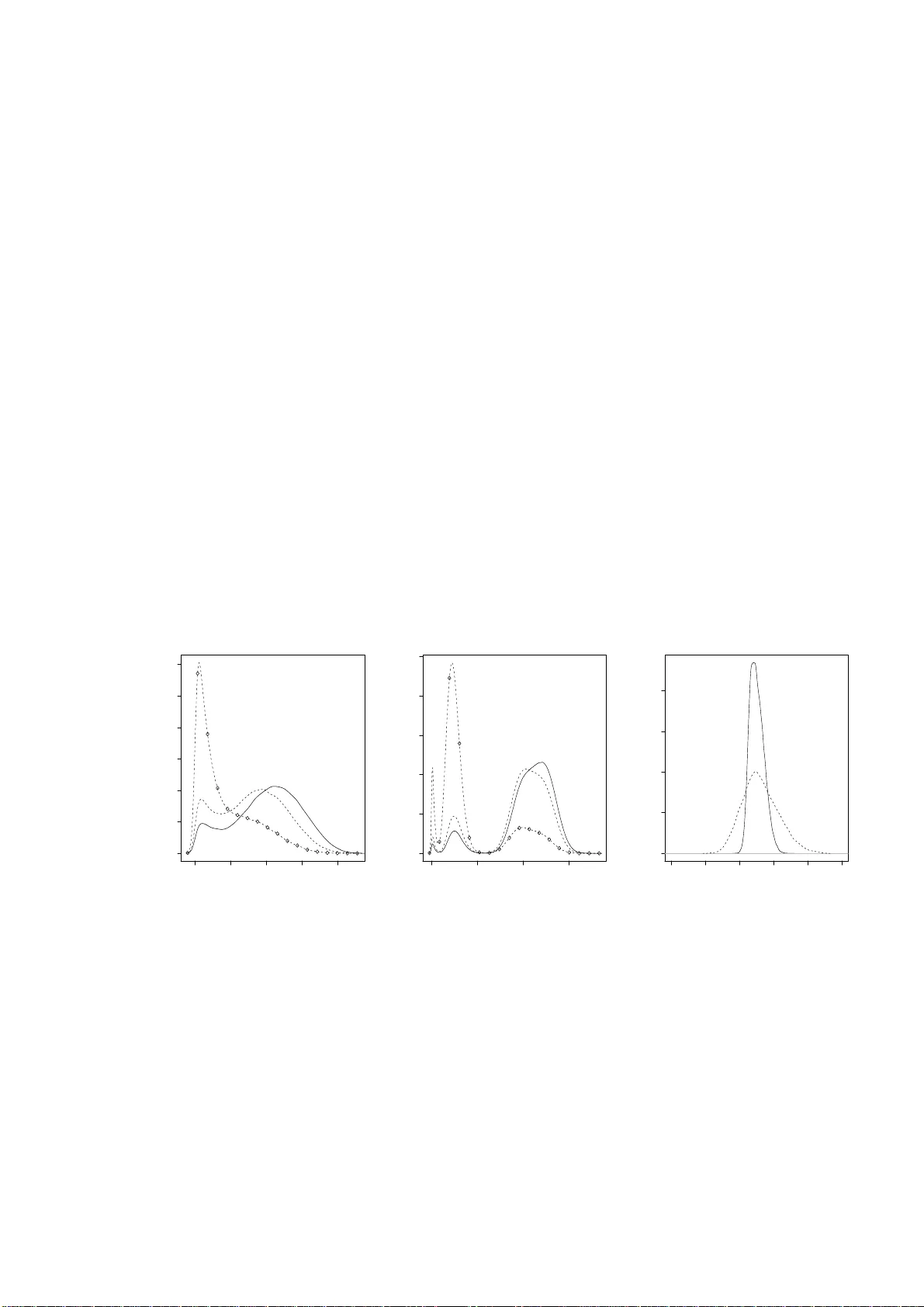
Retrosp ectiv e Mark o v c hain Mon te Carlo metho ds for Diric hlet pro cess h ierarc hical mo del By OMIR O S P AP ASPILIOPO ULO S AND GARETH O. ROBER TS Dep artment of Statistics, Warwick University, Coventry, CV4 7AL, U.K. O.P apasp ilio p oulos@w arw ic k.ac.uk, Gareth.O.Rob erts@w arwick.ac .uk SUMMAR Y Inference for Diric hlet p rocess hierarchica l mo dels is t ypically p erf ormed using Mark ov c hain Mon te Carlo metho ds, whic h can b e roughly categ orised into marginal and condi- tional metho ds. The former in tegrate out analytically the infi nite-dimensional comp o- nen t of the hierarc hical mo del and sample from the marginal distr ib ution of the remainin g v ariables using the Gibb s samp ler. Conditional metho ds impute the Diric hlet p ro cess and up date it as a comp onent of the Gibbs sampler. Since this requir es imputation of an infin ite- dimensional pr ocess, implementa tion of the conditional metho d has relied on finite app ro ximations. In this pap er we show how to a void suc h appr oximati ons b y designing t w o no vel Marko v chain Mon te Carlo algo rithms whic h s ample from the exact p osterior distribution of qu antitie s of int erest. Th e appr o ximations are a v oided b y the new tec hniqu e of r etrosp ectiv e s ampling. W e also sh o w how th e algorithms can obtain samples from fun ctio nals of the Diric hlet pr o cess. The marginal and the condi- tional metho ds are compared and a careful sim ulation study is included , wh ic h inv olv es a non-conjugate mo del, d ifferen t datasets and prior sp ecifications. Some keywor ds: Exact sim ulation; Mixture mo dels; Lab el switc hing; Retrosp ectiv e sam- pling; Stick- breaking pr ior 1. Introduction Diric hlet pr ocess hierarc hical mo dels, also kno wn as Diric h let mixture mo dels, are no w standard in semiparametric inference; app licat ions include densit y estimation (M ¨ uller et al., 1 1996), surviv al analysis (Ge lfand & Kottas, 2003), semi-paramet ric analysis of v ari- ance ( M ¨ uller et al., 2005), cluster analysis and p artitio n mo d elling (Qu in tana & Iglesias , 2003), meta-analysis (Bur r & Doss, 2005) and mac hin e learning (T eh et al., 2006). The hierarc h ica l structure is as follo ws. Let f ( y | z , λ ) b e a parametric densit y with param- eters z and λ , let H Θ b e a d istribution indexed by some p arameters Θ and let Be( α, β ) denote the b eta distr ibution with parameters α, β . Then we ha ve Y i | ( Z, K, λ ) ∼ f ( Y i | Z K i , λ ) , i = 1 , . . . , n K i | p ∼ ∞ X j =1 p j δ j ( · ) Z j | Θ ∼ H Θ , j = 1 , 2 , . . . (1) p 1 = V 1 , p j = (1 − V 1 )(1 − V 2 ) · · · (1 − V j − 1 ) V j , j ≥ 2 V j ∼ Be(1 , α ) . Here V = ( V 1 , V 2 , . . . ) and Z = ( Z 1 , Z 2 , . . . ) are ve ctors of indep endent v ariables and are indep endent of eac h other, the K i s are ind ep enden t giv en p = ( p 1 , p 2 , . . . ), and the Y i s are indep endent give n Z and K = ( K 1 , K 2 , . . . , K n ). Therefore, (1) defines a mixture mo del in w hic h f ( y | z , λ ) is m ixed with resp ect to the discrete random probabilit y mea sure P ( dz ), where P ( · ) = ∞ X j =1 p j δ Z j ( · ) , (2) and δ x ( · ) d enotes the Dirac delta m easure cen tred at x . Note th at, the discreteness of P implies a distr ib utional clustering of th e data. The last three lin es in th e hierarch y iden tify P with the Diric h let pro cess with base measur e H Θ and concen tration parameter α ; this r epresen tation is du e to Sethuraman (1994). F or the construction of th e Dirichlet pro cess prior see F erguson (1973,1 974), for prop erties of Diric hlet m ixture mo dels see for example Lo (1 984), F erguson (1983 ), and An toniak (1974 ), and for a recen t arti- cle on mo delling with Diric hlet pr ocesses see Green & Ric hardson (2001). Using more general b eta distribu tions in the last line giv es rise to the r ic h class of stic k-breaking ran- dom measures and th e general hierarc hical f ramew ork in tr odu ced by Ishw aran & J ames 2 (2001). W e ha ve consciously b een v ague ab out the spaces on wh ic h Y i and Z j liv e; it should b e ob vious from th e construction that a great deal of flexibilit y is allo w ed. W e refer to Z j and p j as the p arameters an d the weigh t resp ectiv ely of the j th comp onen t in the mixture, and to K i as th e allo cati on v ariable, whic h determines to whic h comp onent the i th data p oin t is allocated. Note that the p rior on the comp onent w eights p j imp oses a w eak iden tifiability on the mixture comp onent s, in the sense that E ( p j ) ≥ E ( p l ) for any j ≥ l . T hroughout the pap er we use the nomenclature ‘cluster’ to refer to a mixture comp onent with at least one d atum allo cate d to it. Th e h yp erpa- rameters α, Θ an d λ w ill b e consider fix ed until § 3 · 7. W e w ill concent rate on inf erence for the allo cation v ariables, the comp onen t parameters and wei gh ts, and P itself. Inference for Diric hlet mixture mo dels has b een m ade feasible by Gibb s sampling tec hniqu es whic h ha ve b een devel op ed since the semin al work in an unp ublished 1988 Y ale Univ ersit y Ph. D. thesis by M. Escobar. Alternativ e Mon te Carlo sc hemes do exist and includ e the sequential samp lers of Liu (1996) an d Ishw aran & James (2003), and r eferred to as the b lock ed Gibbs s ampler in those p ap er s , the p article filter of F earnhead (2004 ) and the rev ersible jump metho d of Green & Ric h ardson (2001) and Jain & Neal (2004). W e concen trate on Gibbs sampling and related comp onen t wise up dating algorithms. Broadly sp eaking, there are t w o p ossible Gibbs sampling strategies, corresp onding to t wo differen t data augmen tation sc h emes. Th e marginal metho d exploits con venien t mathematical prop erties of the Diric hlet pro cess and integrat es out analytically the ran- dom probabilities p from the hierarc hy . Then, using a Gibbs sampler, it obtains samples from the p osterior distrib ution of the K i ’s and the p aramete rs an d the w eights of the clus- ters. Integ r ating out p indu ces prior dep endence among the K i ’s, and mak es the lab els of the clusters unid en tifiable. This approac h is easily carried out for conjugate mo dels, where fur th er analytic in tegrations are p ossible; (1) is said to b e conjugate when H Θ ( dz ) and f ( y | z , λ ) form a conjugate p air for z . Im plemen tation of the marginal metho d for non-conjugate m odels is considerably more complicated. MacEac hern & M ¨ uller (1998) 3 and Neal (2000) are the state-of-the-art implemen tations in this cont ext. The conditional metho d works with the augmen tation sc h eme d escrib ed in (1). It consists of the imputation of p and Z , and sub sequen t Gibbs sampling from the join t p osterior distribution of ( K , p, Z ). The conditional indep end ence structure created with the imp utatio n of ( p, Z ) assists the sim u ltaneous up dating of large su b sets of the v ari- ables. The cond itio nal metho d was in tr odu ced in Ishw aran & Zarep our (2000), it w as further deve lop ed in Ishw aran & James (2001, 2003) and it has t wo considerable ad- v an tages o v er the marginal metho d. First, it d oes n ot rely on b eing able to int egrate out a nalytically co mp onen ts of the hierarc hical mo del, and therefore it is muc h more flexible for curren t and future elab oratio ns of the basic mo del. Suc h extensions includ e more g eneral stic k-breaking random measures, and m odelling dep endence of the d ata on co v ariates, as for example in Dunson & Park (2006). A second adv ant age is th at in principle it allo ws inference for the laten t random measure P . The implementa tion of th e conditional metho d p oses interesting metho dological c hal- lenges, s ince it requires the imp utation of the infinite-dimensional v ectors p and Z . The mo dus op erandi adv o cat ed in Ish waran & Zarep our (2000) is to app ro ximate th e ve c- tors, and thus the corresp onding Diric hlet p rocess p rior, u sing s ome kind of tru ncatio n, suc h as p ( N ) = ( p 1 , . . . , p N ) and Z ( N ) = ( Z 1 , . . . , Z N ), wh ere N dete rmines the degree of appro ximation. Although in some cases it is p ossible to control the error pr o du ced by suc h truncations (Ishw aran & Zarep our, 2000, 2002; Ish w aran & James, 2001) it would b e desirable to a v oid approximati ons altogether. This pap er introdu ces tw o implementa tions of the cond itional metho d whic h a v oid an y appro ximation. The prop osed Mark ov c hain Mon te Carlo algorithms are very easily implemen ted and can readily b e extended to m ore general stic k-b r eaking mo dels. The implemen tation of the conditional metho d is ac h iev ed by retrosp ectiv e sampling, w hic h is in tro duced in this pap er. This is a no vel tec hnique which facilitates exact s im ulation in fi nite time in p r oblems wh ic h inv olv e in finite-dimensional pro cesses. W e also show ho w to use retrosp ectiv e sampling in conjunction with our Mark ov c h ain Mon te Carlo 4 algorithms in order to sample fr om the p osterior distribution of fu nctionals of P . W e identi fy a compu tational problem with th e conditional metho d. As a result of the wea k iden tifiability imp osed on the lab els of the mixture comp onen ts, th e p osterior distribution of the r andom m easur e ( p, Z ) is m u ltimodal. Therefore, the Gibbs sam- pler h as to visit all these different mo des. This problem is not eliminated with large datasets, since although the secondary mo des b ecome smaller, the energy gap b etw een the mo des b ecomes b igger, and thus the sampler can get trapp ed in lo w-prob ab ility ar- eas of the state-space of ( p, Z ). W e design tailored lab el-switc hing mo ves w h ic h improv e significan tly the p erformance of our Mark o v c hain Mon te Carlo algorithm. W e also contrast our retrosp ectiv e Marko v c hain Mon te Carlo algorithm with state- of-the-art imp lementat ions of the m arginal metho d for non-conjugate mo dels in terms of th eir Mon te Carlo efficiency . In particular w e consider the no-gaps algorithm of MacEac hern & M ¨ uller (1998) and Algorithms 7 and 8 of Neal (2000). This comparison sheds light on the relativ e merits of the marginal and cond itional metho d in mo dels where th ey can b oth b e applied. W e fin d that the marginal metho ds slightl y outp erform the conditional. Since the original s u bmission of this pap er, the retrosp ectiv e sampling ideas we in tr o- duce here ha v e b een found ve ry useful in extensions of the Diric hlet pro cess h ierarc hical mo del (Dunson & P ark, 2006; Griffin, 2006), and in the exact sim ulation of diffusion pro cesses; see for example Besk os et al. (2006b). 2. Retrospective sampling from the Dirichlet process pr ior Consider the task of simulating a sample X = ( X 1 , . . . , X n ) fr om the Dirichlet pro cess prior (2). Suc h a sample h as the pr operty that X i | P ∼ P , X i is indep endent of X l conditionally o n P for eac h l 6 = i , i, l = 1 , . . . , n , and P is the Diric h let p rocess w ith concen tration parameter α and base measure H Θ . This section introd u ces in a simple con text the tec h nique of retrosp ecti v e sampling and th e tw o differen t computational approac hes, marginal and co nditional, to inference for Diric hlet pro cesses. Th er e are 5 essen tially t wo different wa ys of obtaining X . The sample X can b e sim ulated d irectly fr om its m arginal distr ib ution. When P is marginalised the joint distribu tion of the X i s is known and it is describ ed by a P´ oly a urn sc heme (Blac kw ell & MacQueen, 1973; F erguson, 1973). In p articular, let K i b e an allocation v ariable a sso ciate d with X i , where K i = j if and only if X i = Z j . Ther e- fore, the K i ’s decide wh ic h comp onen t of th e in finite series (2) X i is asso ciate d with. Conditionally on P the K i ’s are ind ep end en t, with pr( K i = j | p ) = p j , for all i = 1 , . . . , n, j = 1 , 2 , . . . . (3) The marginal pr ior of K = ( K 1 , . . . , K n ) is obtained b y the follo wing P´ oly a urn sc heme: pr( K i = j | K 1 , . . . , K i − 1 ) = n i,j ( α + i − 1) , if K l = j for some l < i , pr( K i 6 = K l for all l < i | K 1 , . . . , K i − 1 ) = α ( α + i − 1) , (4) where n i,j denotes the size of the set { l < i : K l = j } . Thus, the probabilit y that the i th sample is asso ciated with the j th comp onen t is prop ortional to the num b er of samples already asso ciate d with j , whereas with probabilit y α/ ( α + i − 1) the i th sampled v alue is asso ciated with a new comp onen t. Note that, whereas in (3 ) the lab els j are iden tifiable, in (4) the lab els of the clusters are totally arbitrary . Simulatio n of X from its marginal d istribution proceeds in foll o wing wa y . Set K 1 = 1, although an y other lab el could b e c h osen; simulate φ 1 ∼ H Θ ; and set X 1 = φ 1 . F or i > 1, let c denote the n um b er of existing clusters; simulate K i conditionally on K 1 , . . . , K i − 1 according to the probabilities (4), where j = 1 , . . . , c ; if K i = j then set X i = φ j , and otherwise set c = c + 1, sim ulate φ c ∼ H Θ indep endently of an y previously dra w n v alues, and set X i = φ c . A t the end of this pro cedure φ F = ( φ 1 , . . . , φ c ) are the parameters of the mixture comp onen ts whic h are asso ciated with at least one data p oint. Th e indexing 1 , . . . , k is arb itrary and it is n ot feasible to map these φ j ’s to the Z j ’s in th e definition of the Diric hlet p rocess in (2). Alternativ ely , X can b e s im ulated follo win g a tw o-step h ierarchical p r ocedur e. Ini- tially , a realisation of P is simulated, and then w e simulate indep endently n allo cation 6 v ariables according to (3) and we set X i = Z K i . Ho wev er, simulati on of P entai ls the generation of the in finite vec tors p and Z , which is infeasible. Nev ertheless, this pr ob lem can b e a vo ided with th e f ollo wing r etrosp ectiv e sim ulation. The stand ard m ethod for sim u lati ng from the discrete distribution defined in (3) is first to sim ulate U i from a uniform distribu tion on (0 , 1), and then to set K i = j if and only if j − 1 X l =0 p l < U i ≤ j X l =1 p l , (5) where w e define p 0 = 0; this is the inv erse cumulat iv e distribu tion fun ction metho d for discrete random v ariables; see for example Ripley (1987, § 3.3). Retrosp ectiv e sampling simply exchanges the order of simulation b etw een U i and the pairs ( p j , Z j ). Rather than sim u lati ng fi rst ( p, Z ) and then U i in ord er to c h ec k (5), we fir st sim ulate the decision v ariable U i and th en pairs ( p j , Z j ). If for a giv en U i w e need more p j ’s than we currently ha ve in ord er to c hec k (5), then we go bac k and simulat e pairs ( p j , Z j ) ‘retrospectiv ely’, unt il (5) is satisfied. The algorithm pr oceeds as follo ws. ALGORITHM 1. R etr osp e ctive sampling fr om the Dirichlet pr o c ess prior Step 1 . Simulate p 1 and Z 1 , and set N ∗ = 1 , i = 1 and p 0 = 0 . Step 2 . R ep e at the fol lowing until i > n . Step 2.1 . Simulate U i ∼ Un [0 , 1] Step 2.2 . If (5) is true f or some k ≤ N ∗ then set K i = k , X i = Z k , for i = i + 1 , and go to Step 2 . Step 2.3 . If (5) i s not true for any k ≤ N ∗ then set N ∗ = N ∗ + 1 , j = N ∗ , simulate p j and Z j , and go to Step 2.2 . In this notation, N ∗ k eeps trac k of ho w far into the infinite sequence { ( p j , Z j ) , j = 1 , 2 , . . . } we h a v e visited du ring the simulati on of the X i ’s. Note that the retrosp ectiv e sampling can b e easily im p lemen ted b ecause of the Marko vian str ucture of the p j ’s and the ind ep end ence of the Z j ’s. A similar scheme w as adv o cated in Doss (1994). The pr evious simulati on sc h eme illus trate s the m ain principle b ehin d retrosp ectiv e 7 sampling: although it is imp ossible to sim u late an infinite-dimensional rand om ob ject w e migh t still b e able to tak e d ecisio ns whic h dep end on suc h ob jects exactly a v oiding any appro ximations. The success of the approac h will dep end on whether or not the decision problem can b e f orm ulated in a wa y that in volv es fi nite-dimensional summaries, p ossibly of r an d om dimens ion, of the random ob ject. In th e p revious to y example w e form u late d the problem of simulati ng d ra ws from the Diric h let pro cess p rior as the problem of com- paring a uniform random v ariable w ith p artial sums of the Diric hlet rand om measur e. This facilitated the simulati on of X in fi nite time a voi ding appr o ximation err ors . In gen- eral, the retrosp ectiv e simulatio n scheme w ill require at th e first s tage simulation of b oth the decision v ariable and certain fin ite- dimensional su mmaries of the infin ite- dimensional random ob ject. Thus, at th e s econd stage w e will n eed to sim ulate r etrosp ect iv ely from the distribution of th e rand om ob ject conditionally on th ese su mmaries. T h is conditional sim u lati on will t ypically b e m u c h more elab orate than the illustration w e ga ve here. W e shall see in § 3 that these ideas extend to p osterior sim ulation in a computationally feasible wa y . Ho w ever, th e details of the metho d for p osterior s imulation are far more complicated than the simple metho d giv en ab o ve. 3. The retrospective cond itional method for posterior simula tion 3 · 1 Posterior infer enc e When w e fit (1) to data Y = ( Y 1 , . . . , Y n ), there are a num b er of quant ities ab out which w e ma y wan t to mak e p osterior in f erence. These includ e the classification v ariables K i , whic h can b e used to classify the data in to clusters, the num b er of clusters in the p opula- tion, the clus ter p aramete rs { Z j : K i = j for at least one i } and the cluster probabilities { p j : K i = j for at least one i } , the hyp erparameters α, Θ and λ , the predictiv e d istribu- tion of futur e data, and the ran d om measure P itself. None of the existing metho ds can pro vide samples from the p osterior distribution of P without resorting to some kind of appro ximation; see f or example Gelfand & Kottas (2002) f or some suggestions. Ho we v er, exact p osterior simulat ion of finite-dimensional distribu tions and fu nctionals of P migh t 8 b e feasible; see § 3 · 6. Mark o v c hain Mont e C arlo tec hn iques ha v e b een dev elop ed for sampling-based exp lo- ration of the p osterior distribu tions outlined ab o ve . The conditional metho d (Is hw aran & Zarep our, 2000) is b ased on an augment ation sc heme in wh ic h the random probabilities p = ( p 1 , p 2 , . . . ) and the comp onent parameters Z = ( Z 1 , Z 2 , . . . ) are imp uted and the Gibbs sampler is used to sample from the join t p osterior distribution of ( K, p, Z ) according to the full-conditional distribu tions of the v ariables. Ho w ever, the fact that p and Z ha ve coun tably infin ite element s p oses a ma jor c hallenge. Ishw aran & Z arep ou r (2000) adv o cated an appro ximation of these vec tors, and therefore an appr o ximation of th e corresp onding Diric hlet pro cess p r ior. F or instance a tru n cati on of the Seth uraman rep - resen tation (2) could b e adopted, e.g. p ( N ) = ( p 1 , . . . , p N ) and Z ( N ) = ( Z 1 , . . . , Z N ), where N determines the degree of appr o ximation. In this section we sho w ho w to a vo id any such appro ximation. The fi rst step of our solution is to p aramete rise in terms of ( K, V , Z ), where V = ( V 1 , V 2 , . . . ) are the b eta random v ariables u s ed in the stic k-br eaking constru ctio n of p . W e will construct algorithms w h ic h effectiv ely can return samples fr om the p osterior distribu tion of these v ectors, by s imulating iterativ ely from th e full conditional p osterior d istributions of K , V and Z . Note th at we can rep lac e d irect sim u lati on from the conditional distributions w ith an y up dating mec hanism, suc h as a Metropolis-Hastings ste p, whic h is inv arian t with resp ect to these conditional distrib u tion. Th e stationary d istr ibution of this more general comp onen twise- up dating samp ler is still the joint p osterior d istr ibution of ( K, V , Z ). W e no w in tr o du ce some notation. F or a giv en configuration of the classification v ariables K = ( K 1 , . . . , K n ), we d efine m j = n X i =1 1 { K i = j } , j = 1 , 2 , . . . , to b e the n um b er of data p oint s allo cated to the j th comp onent of the mixtur e. Moreo v er, 9 again for a give n configuration of K let I = { 1 , 2 , . . . } I ( al ) = { j ∈ I : m j > 0 } I ( d ) = { j ∈ I : m j = 0 } = I − I ( al ) . Therefore, I represent s all comp onents in the infinite mixture, I al is the s et of all ‘aliv e’ comp onen ts and I ( ) . the set of ‘dead’ comp onen ts, wh er e w e call a comp onent ‘aliv e’ if some data h a v e b een allocated to it. The corresp onding p artition of Z and V will b e denoted by Z (al) , Z ( ) . , V (al) and V ( ) . . The implementa tion of our Marko v c hain Monte Carlo algorithms relies on the r esults con tained in the follo win g Pr oposition, whic h describ es the full conditional p osterior distributions of Z , V and K . Prop osition 1. L et π ( z | Θ ) b e the density of H Θ ( dz ) . Conditional ly on ( Y , K, Θ , λ ) , Z is indep endent of ( V , α ) and it c onsists of c onditional ly indep endent elements with Z j | Y , K , Θ , λ ∼            H Θ , for al l j ∈ I ( ) . Q i : K i = j f ( Y i | Z j , λ ) π ( Z j | Θ) for al l j ∈ I (al) , Conditional ly on ( K, α ) , V is indep endent of ( Y , Z , Θ , λ ) and i t c onsists of c onditional ly indep endent elements with V j | K, α ∼ Be m j + 1 , n − j X l =1 m l + α ! for al l j = 1 , 2 , . . . . Conditional ly on ( Y , V , Z, λ ) , K is indep endent of (Θ , α ) and it c onsist of c onditional ly indep endent elements with pr { K i = j | Y , V , Z , λ } ∝ p j f ( Y i | Z j , λ ) , j = 1 , 2 , . . . . The pro of of the Pr op osition follo ws directly from the conditional ind epen dence struc- ture in the mod el and the stic k-breaking representati on of the Diric hlet pro cess; see Ish w aran & James (2003) for a pro of in a m ore general con text. 10 The conditional indep end ence stru cture in the mo del effects the simultaneo us sam- pling of an y fin ite su bset of p airs ( V j , Z j ) according to their fu ll cond itio nal distributions. Sim ulation of ( Z j , V j ) wh en j ∈ I ( ) . is trivial. When dealing with non-conjugate mo dels, the distrib ution of Z j for j ∈ I (al) will t ypically not b elong to a k n o wn family and a Metrop olis-Ha stings step m ight b e used instead to carry out this simulation. Note th at samples from the fu ll conditional p osterior d istr ibution of p j ’s are obtained u s ing samples of ( V h , h ≤ j ) and the stic k-breaking represen tation in (1). The K i ’s are conditionally indep endent giv en Z and V . Ho wev er, the normalising constan t of the f ull cond itional probabilit y mass fu nction of eac h K i is in tractable: c i = ∞ X j =1 p j f ( Y i | Z j , λ ) . The intract abilit y stems from the f act that an in finite sum of random terms needs to b e computed. At th is stage one could resort to a fi nite appro ximation of the sums, bu t we wish to a v oid this. The unav ailabilit y of the n ormalising constan ts ren d ers sim u latio n of the K i ’s highly non trivial. T h erefore, in order to constr u ct a conditional Mark o v c hain Monte Carlo algorithm we need to find w ays of sampling from the conditional distribution of the K i ’s. 3 · 2 A r etr osp e ctive quasi- indep endenc e M e tr op olis-Hastings sampler for the al lo c ation variables One sim p le and effectiv e w a y of a v oiding the computation of the normalising constants c i is to replace d irect s imulation of the K i s w ith a Metrop olis-Hastings step. Let k = ( k 1 , . . . , k n ) denote a configuration of K = ( K 1 , . . . , K n ), and let max { k } = max i k i b e the maximal elemen t of the v ector k . W e assu me that w e hav e already obtained samples from the co nditional p osterior distribution of { ( V j , Z j ) : j ≤ max { k }} giv en K = k . Note that the d istribution of ( V j , Z j ) conditionally on Y and K = k is s imply the pr ior, V j ∼ Be( α, 1) , Z j ∼ H Θ , for any j > max { k } . 11 W e will d escribe an up dating sc heme k 7→ k ∗ whic h is inv ariant with resp ect to the full conditional d istr ibution of K | Y , Z , V , λ . T he sc heme is a comp osition of n Metrop olis-Ha stings steps which u p date eac h of th e K i s in turn . Let k ( i, j ) = ( k 1 , . . . , k i − 1 , j, k i +1 , . . . , k n ) b e the v ector pro duced from k b y sub stituting the i th element by j . When up dating K i , the sampler p rop oses to mov e fr om k to k ( i, j ), w here the prop osed j is generated fr om the pr obabilit y mass fu nction q i ( k , j ) ∝            p j f ( Y i | Z j , λ ) , for j ≤ m ax { k } M i ( k ) p j , for j > m ax { k } . (6) The normalising constan t of (6) is ˜ c i ( k ) = max { k } X j =1 p j f ( Y i | Z j , λ ) + M i ( k )   1 − max { k } X j =1 p j   , whic h can b e easily computed giv en { ( p j , Z j ) : j ≤ max { k }} . Note th at, for j ≤ m ax { k } , q i ( k , j ) ∝ pr( K i = j | Y , V , Z, λ ), while, for j > max { k } , q i ( k , j ) ∝ pr( K i = j | V ). Here M i ( k ) is a user-sp ecified parameter wh ic h con trols the p robabilit y of prop osing j > max { k } , and its c hoice will b e discus sed in § 3 · 3 . According to th is prop osal distribution the i th data p oint is prop osed to b e r e- allocated to one of the alive clusters j ∈ I (al) with probabilit y prop ortional to the cond i- tional p osterior probabilit y pr( K i = j | Y , V , Z , λ ). Allo cation of th e i th data p oint to a new comp onen t can b e accomplished in tw o wa ys: b y prop osing j ∈ I ( ) . for j ≤ m ax { k } according to the conditional p osterior p r obabilit y mass fun ctio n and by prop osing j ∈ I ( ) . for j > max { k } according to the prior p robabilit y mass f unction. Therefore, a careful calculatio n yields that th e Metrop olis-Hastings acceptance pr obabilit y of the transition 12 from K = k to K = k ( i, j ) is α i { k , k ( i, j ) } =                          1 , if j ≤ ma x { k } and ma x { k ( i, j ) } = max { k } min  1 , ˜ c i ( k ) M { k ( i,j ) } ˜ c i { k ( i,j ) } f ( Y i | Z k i ,λ )  , if j ≤ max { k } and max { k ( i, j ) } < max { k } min n 1 , ˜ c i ( k ) f ( Y i | Z j ,λ ) ˜ c i { k ( i,j ) } M ( k ) o , if j > ma x { k } . Note th at prop osed re-allo catio ns to a comp onen t j ≤ max { k } are accepted with prob- abilit y 1 pr o vided that max { k ( i, j ) } = max { k } . If the prop osed mov e is accepted, w e set k = k ( i, j ) and p ro cee d to the u p dating of K i +1 . The comp osition of all these steps yields the u p dating mechanism for K . Sim ulation from the pr oposal distribu tion is ac hieved by retrosp ectiv e sampling. F or eac h i = 1 , . . . , n , we sim u late U i ∼ Un[0 , 1] and prop ose to set K i = j , where j satisfies j − 1 X l =0 q i ( k , l ) < U i ≤ j X l =1 q i ( k , l ) , (7) with q i ( k , 0) ≡ 0. If (7) is not satisfied f or an y j ≤ max { k } , then we start c h ec king the condition for j > m ax { k } unt il it is satisfied. This will requ ire the v alues of ( V l , Z l ) , l > max { k } . If these v alues hav e not already b een s im ulated in the previous steps of the algorithm, they are simulated r etrospectiv ely from their prior distribution when they b ecome needed. W e therefore h a v e a retrosp ectiv e Mark o v chain Monte Carlo algorithm for sampling from the joint p osterior distribution of ( K , V , Z ), which is su mmarised b elo w. ALGORITHM 2. R etr osp e ctive M arko v chain M onte Carlo Give an initial al lo c atio n k = ( k 1 , . . . , k n ) , and set N ∗ = max { k } Step 1 . Simulate Z j fr om its c onditiona l p osterior, j ≤ max { k } . Step 2.1 Simulate V j fr om its c onditional p osterior, j ≤ max { k } . Step 2.2 Calculate p j = (1 − V 1 ) · · · (1 − V j − 1 ) V j , j ≤ max { k } . Step 3.1 . R ep e at the f ol lowing until i > n . 13 Step 3.2 . Simulate U i ∼ Un [0 , 1] Step 3.3.1 If (7) is true for some j ≤ N ∗ then set K i = j with pr ob ability α i { k , k ( i, j ) } , otherwise le ave it unchange d. Set i = i + 1 and go to Step 3.1 . Step 3.3.2 If (7) i s not true for any j ≤ N ∗ , se t N ∗ = N ∗ + 1 , j = N ∗ . Simulate ( V j , Z j ) fr om the prior, set p j = (1 − V 1 ) · · · (1 − V j − 1 ) V j and go to Step 3.3.1 Step 3.4 . Set N ∗ = max { k } and go to Step 1 . Note th at b oth max { k } and N ∗ c hange durin g th e up dating of the K i ’s, with N ∗ ≥ max { k } . Th u s, th e prop osal distribution is adapting itself to impro ve appro ximation of the target distribution. A t the early stages of the algorithm N ∗ will b e large, bu t as the cluster structure starts b eing iden tified by the d ata then N ∗ will tak e m u c h smaller v alues. Nev ertheless, the adaptation of the algorithm do es not violate the Mark ov prop ert y . It is recommended to up d ate the K i ’s in a random order, to a vo id using systematically less efficien t prop osals for some of the v ariables. The algorithm w e hav e constructed up d ates all the allo cation v ariables K but only a random subset of ( V , Z ), to b e p recise { ( V j , Z j ) , j ≤ N ∗ } . Ho w ev er, pairs of the complemen tary set { ( V j , Z j ) , j > N ∗ } can b e s im ulated when and if they are needed retrosp ectiv ely from the prior d istribution. This sim ulation ca n b e p erformed off-line after th e completion of the algorithm. In this sense, our algorithm is capable of exploring the joint d istribution of ( K, V , Z ). 3 · 3 A c c eler ation s of the main algorithm There are sev eral simple mo difications of the retrosp ectiv e Marko v c hain Mon te C arlo algorithm whic h can imp ro v e significant ly its Mon te Carlo efficiency . W e fir st discuss the c h oic e of th e u ser-sp ecified parameter M i ( k ) in (6). This p aram- eter relates to the probabilit y , ρ sa y , of prop osing j > max { k } , where ρ =  1 − P max { k } j =1 p j  M i ( k ) c i (max { k } ) . If it is desired to prop ose co mp onen ts j > max { k } a sp ecific p r op ortion of the time 14 then the equation ab o v e can b e s olved for M i ( k ). F or example, ρ = α/ ( n − 1) is the probabilit y of prop osing new clus ters in Al gorithm 7 of Ne al (2 000). W e recommend a c hoice of M i ( k ) whic h guaran tees that the prob ab ility of p rop osing j > max { k } is greater than the pr ior pr ob ab ility assigned to the set { j : j > max { k }} . Thus M i ( k ) should satisfy max { k } X j =1 p j f ( Y i | Z j , φ ) + M i ( k )   1 − max { k } X j =1 p j   ≤ M i ( k ) . This inequalit y is satisfied b y setting M i ( k ) = max { f ( Y i | Z j , φ ) , j ≤ max { k }} . (8) Since (6) resembles an indep endence samp ler for K i , (8) is advisable from a theoretical p ersp ectiv e. Mengersen & Twe edie (1996) ha v e sho wn that an indep endence sampler is geometrically ergo dic if and only if the tails of the prop osal d istribution are h eavie r than the tails of the target distribu tion. The choice of M i ( k ) according to (8) ensu res that the tails of th e prop osal q i ( k , j ) are hea vier than the tails of the target p robabilit y pr { K i = j | Y , p, Z , λ } . No te th at when M i ( k ) is c hosen according to (8) then ρ is rand om. In sim ulation studies we ha v e disco vered that the d istribution of ρ is v ery skew ed and the c hoice according to (8) leads to a faster mixing algorithm than alternativ e sc h emes with fixed ρ . Another int eresting p ossibilit y is to up date Z and V after eac h up date of the allo- cation v ariables. Before Step 3.2 of Algorithm 2 w e sim ulate Z ( ) . from the pr ior and lea v e Z (al) unc hanged. Moreo ve r, w e can sy n c hronise N ∗ and max { k } . Theoretically , this is ac hiev ed by p retending to up date { V j , j > max { k }} from the prior b efore S tep 3.2. In pr acti ce, the only adjustment to the existing algorithm is to set N ∗ = max { k } b efore Step 3.2. These extra u p dates h a v e the compu tatio nal adv antag e of storing only Z (al) and { V j , j ≤ max { k }} . In add ition, simulatio ns hav e v erifi ed that these extra up- dates impr o v e significan tly th e mixing of th e algorithm. Moro ver, one can allo w more comp onen ts j ∈ I ( ) . to b e prop osed according to the p osterior probabilit y mass function b y c hanging max { k } in (6 ) to max { k } + l , for some fixed in teger l . In that case the 15 acceptance pr obabilit y (3 · 2) needs to b e sligh tly mo dified , but we ha ve not found gains from such adju stmen t. 3 · 4 Multimo dality and lab el-switching moves The most s ignifi can t and crucial m odifi cat ion of the algorithm we hav e in tro duced is the addition of lab el-switc hing mo ves. T hese mo ves will h a v e to b e included in an y implemen tation of the conditional metho d whic h up dates the allo cation v ariables one at a time. The augmen tation of p in the cond itio nal m ethod make s the comp onen ts in the infinite mixture (1) wea kly ident ifiable, in the sens e that E { p j } ≥ E { p l } for an y j ≥ l , but t here is nonnegligible p r ior probabilit y th at p l > p j , in p articular w hen | l − j | is small. As a result the p osterior distribu tion of ( p, Z ) exhibits m ultiple m odes. In ord er to h ighligh t this phenomenon we consider b elo w a simplified s cenario, bu t we refer to § 4 for an illustration in the con text of p osterior inference for a sp ecific non-conjugate Diric hlet pro cess hierarc h ical mo del. In p articular, assume that we ha v e actually observ ed a sample of size n from the Diric hlet pro cess X = ( X 1 , . . . , X n ) using the notation of § 2. This is the limiting case of (1) where the observ atio n den sit y f ( y | z , λ ) is a p oint mass at z . In this ca se we directly observe the allocation of the X i ’s into c , say , clusters, eac h of size n l , sa y , where P c l =1 n l = n . T he common v alue of the X i ’s in eac h cluster l giv es pr eci sely the parameters φ l of the corresp onding cluster l = 1 , . . . , c . Ho w ever, ther e is still uncertain t y regarding the comp onent probab ilities p j of the Diric hlet p ro cess w hic h generated the sample, and the index of the comp onen t f or whic h eac h cluster has b een generated. Let K l , l = 1 , . . . , c denote these ind ices for eac h of the clusters. W e can construct a Gibbs sampler f or exploring the p osterior distr ibution of p and ( K 1 , . . . , K c ): this is a nont rivial sim u lati on, and a v ariation of the retrosp ectiv e Marko v chain Monte Carlo algorithm has to b e u s ed. Figure 1 s ho ws the p osterior d ensities of ( p 1 , p 2 , p 3 ) when n = 10 and c = 3 with n 1 = 5 , n 2 = 4 , n 3 = 1, and when n = 100 and c = 3 with n 1 = 50 , n 2 = 40 , n 3 = 10. In b oth cases we to ok α = 1. 16 Note th at the p osterior distribu tions of the p j s exhib it multiple mo des, b ecause the lab els in the mixture are only wea kly iden tifiable. Note that the secondary mo des b ecome less prominent f or larger samp les, but the energy gap b et ween the mo des increases. In con trast, the pr obabilit y of the largest comp onen t, max { p j } , has a unimo dal p osterior densit y . T h is is shown in the right p anel of Figure 1(c); sim ulation from this density has b een ac hieve d b y retrosp ectiv e sampling, see § 3 · 6. In general, in the conditional metho d the Mark ov c hain Mon te C arlo algorithm has to explore multimod al p osterior distributions as those shown in Figure 1. Th erefore, w e n eed to add lab el-switc hing mov es wh ic h assist the algorithm to ju mp across mo des. This is p articularly imp ortan t f or large datasets, where the mo des are s eparated by ar- eas of negligible p robabilit y . A careful ins p ecti on of the pr oblem suggests t wo types of mo ve. The first prop oses to change the labels j and l of t w o randomly c hosen com- p onen ts j, l ∈ I (al) . The probabilit y of such a c hange is accepted with pr obabilit y min { 1 , ( p j /p l ) m l − m j } . This prop osal has high acceptance probabilit y if the t w o com- p onen ts ha v e similar w eigh ts; the probabilit y is indeed 1 if p j = p l . On the other hand, note that th e probability of acceptance is small wh en | m l − m j | is close to 0. The s eco nd mo ve pr oposes to c hange the lab els j and j + 1 of t w o neighbour in g comp onent s but at th e same time to exc hange V j with V j +1 . This change is accepted with prob ab ility min { 1 , (1 − V j +1 ) m j / (1 − V j ) m j +1 } . Th is prop osal is very effectiv e for swapping the lab els of v ery un equal clusters. F or example, it will alwa ys accept when m j = 0. On th e other hand, if | p j − p j +1 | is sm all, then the pr op osal w ill b e rejected with high probabilit y . F or example, if V j ≏ 1 / 2, V j +1 ≏ 1, and m j ≏ m j +1 , then th e prop osal attempts to allo cate m j is allo cat ed to a comp onen t of negligible weigh t, Q j − 1 l =1 (1 − V l )(1 − V j +1 ) V j . Thus, the t w o mo ves we hav e suggested are complemen tary to eac h other. Extensiv e simulation exp erimen tation has rev ealed that suc h mov es are cru cial . The in tegrated auto correlat ion time, see § 4 for defin itio n, of the up dated v ariables can b e reduced by as m u c h as 50-9 0%. The problem of multimod alit y has also b een add ressed in a recen t p ap er by P orteous et al. 17 (2006). 3 · 5 Exact r etr osp e ctive sampling of the al lo c ation variables It is p ossible to a void the Metrop olis-Hastings step and simulat e directly from the con- ditional p osterior distribu tio n of the allo cation v ariables. This is facilitated by a general retrosp ectiv e sim ulation sc heme for sampling discrete random v ariables w hose p r obabilit y mass function dep end s on the Diric hlet random measure. W e can f orm ulate the problem as on e of simulati ng a discrete random v ariable J , according to the distribution sp ecified by the probabilities r j := p j f j P ∞ j =1 p j f j , j = 1 , 2 , . . . . (9) The f j ’s are assumed to b e p ositiv e and indep end ent random v ariables, also in dep enden t of the p j ’s, whic h are giv en by the stic k-breaking rule in (1), although more general sc hemes can b e incorp orated in our metho d. The retrosp ectiv e sampling scheme of § 2 cannot b e applied here, since the norm alising constant of (9), c = P p j f j , is un kno wn. In the sp ecific application we hav e in mind, f j = f ( Y i | Z j , λ ) for eac h allo cation v ariable K i w e wish to up d ate. Nev ertheless, a retrosp ectiv e scheme can b e ap p lied if we can construct t wo b ou n ding sequences { c l ( k ) } ↑ c and { c u ( k ) } ↓ c , where c l ( k ) and c u ( k ) can b e calculated s im p ly on the basis of ( p 1 , Z 1 ) , . . . , ( p k , Z k ). Let r u,j ( k ) = r j /c l ( k ) and r l,j ( k ) = r j /c u ( k ). Then w e first sim ulate a uniform U and then we s et J = j when j − 1 X m =1 r u,m ( k ) ≤ U ≤ j X m =1 r l,m ( k ) . (10) In this algorithm k sh ould b e increased, and the p j ’s and f j ’s sim ulated retrosp ectiv ely , unt il (10) can b e verified for some j ≤ k . Therefore, sim u latio n from unn orm alise d d iscrete probabilit y d istributions is feasible pro vided the b ound in g sequences can b e app r opriately constructed. It turn s out that this construction is generally very c hallenging. In this pap er w e will only tac kle the simple case in whic h there exists a constan t M < ∞ su c h that f j < M for all j al most 18 surely . In our application this corresp onds to f ( y | z , λ ) b eing b ounded in z . I n th at case one can simply tak e c l ( k ) = k X j =1 p j f j c u ( k ) = c l ( k ) + M   1 − k X j =1 p j   . When lim s up f j = ∞ almost s urely , an alternativ e construction has to b e d evised, whic h inv olv es an app r opriate coupling of the f j ’s. This constru ctio n is elab orate and mathematicall y int ricate, and w ill b e rep orted elsewhere. 3 · 6 Posterior infer enc e for functionals of Dirichlet pr o c esses Supp ose w e are int erested in estimating the p osterior distrib ution of I = Z X g ( x ) P ( dx ) , for some real-v alued function g , where X denotes the space on wh ic h the comp onen t parameters Z j are defin ed and P is the Dirichlet r andom measure (2), giv en data Y f rom the hierarc hical mo del (1). Our imp lemen tation of the conditional metho d sh o ws that sim u lati on fr om the p osterior distrib ution of I is as d ifficult as the simulation from its prior. Let { ( V j , Z j ) , j ≤ max { k }} b e a sample obtained using the retrosp ectiv e Mark o v c hain Monte Carlo algorithm. W e assume that the sample is tak en when the c h ain is ‘in s tat ionarit y’, i.e. after a sufficien t n u m b er of initial iterations. Given the V j ’s we can compute the corresp onding p j , j ≤ max { k } . Reca ll that Z j ∼ H Θ and V j ∼ Be(1 , α ) for all j > max { k } . Th en we hav e the follo wing r epresen tation for the p osterior distribu tion of I : a d ra w from I | Y can b e represent ed as max { k } X j =1 f ( Z j ) p j + ∞ X j = max { k } +1 f ( Z j ) p j = max { k } X j =1 f ( Z j ) p j + I Q max { k } l =1 (1 − V l ) . This is equ alit y in distribution, w h ere I is a dra w f rom from the prior distribution of I . Inference for lin ear functionals of the Dirichlet pr ocess wa s initiated in C ifarelli & Regazzini 19 (1990) and sim u lati on asp ects hav e b een considered, for example in Guglielmi & Tw eedie (2001) and Gu glielmi et al. (2002). Our algorithm can also b e used f or the simulatio n of non-linear functionals und er the p osterior distrib u tion. As an illustr ative example consider p osterio r sim ulation of the predominant sp ecies corresp onding to J s uc h that p J ≥ p l for all l = 1 , 2 , . . . . This can b e ac hiev ed as follo w s giv en a sample { ( V 1 , Z 1 ) , j ≤ max { k }} obtained with an y of our conditional Marko v c hain Mon te Carlo algorithms. Let J = arg max { j ≤ N ∗ } p j , where N ∗ = max { k } . Then, it can b e seen that if 1 − P N ∗ j =1 p j < p J then J is the p redominan t sp ecie. Therefore, if 1 − Π N ∗ > p J , we rep eat the follo w ing pro cedure u n til the condition is satisfied: increase N ∗ , sim ulate pairs ( Z N ∗ , V N ∗ ) from the p rior, and compu te J . This pro cedure w as used to obtain th e results in Figure 1(c). 3 · 7 Infer enc e for hyp erp ar ameters A s imple mo dification of the retrosp ectiv e algorithms describ ed ab o ve pr o vides the com- putational mac h in ery needed for Ba yesia n inf erence for the h yp erparameters (Θ , α, λ ). If w e assume that appropriate prior d istr ibutions hav e b een c h osen, the aim is to sim ulate the h yp erparameters according to their f ull conditional distributions, thus adding one more step in the retrosp ectiv e Mark o v c h ain Monte Carlo algorithm. Sampling of λ according to its full conditional d istribution is standard. A t first glance, sampling of (Θ , α ) p oses a ma jor complication. Note that, b ecause of the hierarc hical structure, (Θ , α ) are indep endent of ( Y , K ) conditionally up on ( V , Z ). Ho we v er, ( V , Z ) con tains an infin ite amoun t of information ab out ( α, Θ). T h erefore, an algorithm whic h up dated successiv ely ( V , Z , K ) and (Θ , α ) according to th eir full cond itio nal distributions w ould b e reducible. This type of conv ergence problem is n ot uncommon wh en Marko v c hain Mon te Carlo is used to infer ab out hierarc hical mo dels with h idden sto c hastic pro cesses; see P apaspiliop oulos et al. (2003, 2006) for reviews. Ho we v er, the conditional indep endence structure in Z and V can b e used to cir- cum ven t the problem. In effect, instead of up dating (Θ , α ) conditionall y up on ( Z, V ) 20 w e can jointl y u p date (Θ , α, Z ( ) . , V ( ) . ) conditionally u p on ( Z (al) , V (al) ). In pr acti ce, we only need to simulate (Θ , α ) conditionally on ( Z (al) , V (al) ). T hat p oses no complicatio n since ( Z (al) , V (al) ) con tains only finite amount of information ab out the hyperp arameters. It is wo rth mentio ning th at a sim ilar tec hnique for up dating the hyp erparameters was recommended by MacEac h ern & M ¨ uller (1998) for the implemen tation of their no-gaps algorithm. 4. Comp arison betwe en ma r ginal and c onditional metho ds In this section we attempt a comparison in terms of Monte C arlo efficiency b et w een th e retrosp ectiv e Mark ov c hain Monte Carlo algorithm and state-of-the-art implementat ions of the marginal approac h. T o this end w e ha v e carried out a large simulation study part of w h ic h is pr esen ted later in this section. The metho ds are tested on the non- conjugate mo del where f ( y | z ) is a Gaussian d ensit y with z = ( µ, σ 2 ) and H Θ is the pro duct measure N ( µ, σ 2 z ) × IG ( γ , β ); there are no f urther p aramete rs λ indexing f ( y | z ), Θ = ( µ, σ 2 z , γ , β ) and IG ( γ , β ) denotes the in verse Gamma distrib ution with density prop ortional to x − ( γ +1) e − β x . Note th at, in a densit y-estimation con text, this mo del allo ws f or lo cal smo othing; see for example M ¨ uller et al. (1996) and Green & Ric h ardson (2001). An excellen t o verview of d ifferen t imp lemen tations of the marginal approac h can b e found in Neal (2000). Th e most successful implemen tations for non-conju gate mo dels are the so-called no-gaps algorithm of MacEac hern & M ¨ uller (1998) and Algorithms 7 and 8 of Neal (2000), whic h w er e in tro duced to mitigate against certain computational inefficiencies of the no-gaps algorithm. Receiv ed Mark o v chain Mon te Carlo wisdom s u ggest s that marginal samp lers ought to b e preferred to conditional on es. Some limited theory sup p orts this view; see in particular Liu (1994). Ho we v er, it is common for marginalisation to destro y conditional indep endence stru ctur e which usually assists the conditional sampler, sin ce conditionally indep endent comp onen ts are effectiv ely up dated in one blo c k. Thus, it is difficult a priori 21 to decide wh ic h appr oac h is p referable. In our comparison w e ha ve considered different simulat ed datasets and different prior specifications. W e ha v e sim ulated 4 datasets from t wo models. The ‘lepto 100’ and the ‘lepto 1000’ datasets consist r esp ectiv ely of 100 and 1000 d r a ws from the uni- mo dal leptokurtic mixture, 0 . 67 N (0 , 1) + 0 . 33 N (0 . 3 , 0 . 25 2 ). T he ‘bimo d 100’ (‘bimod 1000’) d ataset consists of 100 (1000) d ra ws f r om the bim o dal m ixture, 0 . 5 N ( − 1 , 0 . 5 2 ) + 0 . 5 N (1 , 0 . 5 2 ); we ha ve c hosen these d atase ts follo wing Green & Ric h ard son (2001). I n our s imulation we hav e tak en the dataset s of size 100 to b e subsets of those of size 1000. W e fix Θ in a data-driv en wa y as s u gge sted by Green & Ric hard s on (2001): if R denotes the range o f the d ata , then we set µ = R / 2 , σ z = R, γ = 2 an d β = 0 . 02 R 2 . Data-depen d en t c hoice of hyp erparameters is co mmonly made in mixture models, see for example Ric hardson & Gr een (1997). W e consider thr ee different v alues of α , 0 . 2 , 1 and 5. W e use a Gibbs mo v e to up date Z j = ( Z (1) j , Z (2) j ) f or ev ery j ∈ I (al) : w e up d ate Z (2) j giv en Z (1) j and th e rest, and th en Z (1) j giv en the new v alue of Z (2) j and th e rest. The same sc heme is used to up date the corresp ond ing cluster parameters in the marginal algorithms. W e monitor the conv ergence of four fu nctionals of the u p dated v ariables: the num b er of clusters, M , the deviance D of the estimated d ensit y , and Z (1) K i , for i = 1 , 2 in ‘lepto’ and for i = 2 , 3 in ‘bim o d’. T h ese fu nctionals ha ve b een used in the comparison stud ies in Neal (2000) and Gr een & Ric hard son (2001) to m onitor algorithmic p erf ormance. In b oth cases, the comp onen ts monitored were c hosen to be ones whose allo cations were particularly well- and badly-identified b y the data. The d eviance D is calculated as follo ws D = − 2 n X i =1 log  X j ∈ I (al) m j n f ( Y i | Z j )  ; see Green & Ric hard son (2001) for details. Although we h a v e giv en t he expression in terms of the output of the cond itional algorithm, a similar expression exists given the output of the marginal algorithms. T he deviance is c hosen as a meaningful f unction of sev eral parameters of interest. 22 The efficiency of the s ampler is summarised by rep orting for eac h of the monitored v ariables the estimated inte grated auto correlation time, τ = 1 + 2 P ∞ j =1 ρ j , where ρ j is the lag- j auto correlatio n of the m onitored c hain. This is a standard wa y of measur ing the sp eed of conv ergence of square-in tegrable functions of an ergo dic Mark ov c hain (Rob erts, 1996; Sok al, 19 97) whic h has also b een u sed by Neal (20 00) and Green & R ichardson (2001) in their sim u lati on studies. Recall that the in tegrated auto correlation time is p rop ortional to the asym p totic v ariance of the ergo dic a v erage. In p articular, if τ 1 /τ 2 = b > 1, where τ i is the in tegrated auto correlatio n time of algorithm i for a sp ecific functional, then Algorithm 1 requires roughly b times as many iterations to ac hiev e the same Monte Carlo error a s Alg orithm 2, for the estimati on of the sp ecific functional. Estimation of τ is a notoriously difficult problem. W e hav e follo wed the guidelines in § 3 of Sok al (1997). W e estimate τ by summing estimated auto correlations up to a fi xed lag L , where τ << L << N , and N is the Mon te Carlo sample size. Approximat e standard errors of the estimate can b e obtained; see form ula (3.19) of S ok al (1997). F or the datasets an d pr ior sp ecifications we ha ve consid er ed we ha ve f ou n d that N = 2 × 10 6 suffices in order to assess the relativ e p erformance of the comp eting algorithms. The results of our comparison are rep orted in T ables 1 - 3. W e co n tr ast our ret- rosp ectiv e Mark ov chain Mon te Carlo algorithm with three marginal algorithms: an impro v ed v ersion of the no-gaps algorithm of MacEac hern & M ¨ uller (1998), where we up dated dead-cluster parameters after eac h allo cation v ariable u p date, Algorithm 7 of Neal (2000), and Algorithm 8 of Neal (2000), wher e we u s e three auxiliary states. T he results sho w that Algorithms 7 and 8 p erform b etter than the comp etitors, although the difference among the algorithms is mo derate. In this comparison w e hav e not tak en in to accoun t the computing times of the different metho ds. Our imp lementat ion, w hic h ho wev er did not aim at optimizing compu tatio nal time, in F OR TRAN 77 suggests that no-gaps, Algorithm 7 and the retrosp ectiv e Mark o v c hain Monte Carlo algorithm all ha ve r ou gh ly similar computing times w h en α = 1. Algorithm 8 is more intensiv e than Algorithm 7. The computing time of the r etrosp ective algorithm increases with the v alue 23 of α . Careful insp ection of the outpu t of the algorithms has s u ggest ed a p ossible reason wh y the conditional approac h is outp erformed by the marginal approac hes. This is b ecause it has to explore m u ltiple mo des in the p osterio r distribution of the r an d om measure ( p, Z ); see f or example Figure 2 for results concerning the ‘bimo d’ dataset. On the other hand , the ambiguit y in the cluster lab elling is n ot imp ortant in the m arginal approac hes, wh ich w ork with the un iden tifiable allocation structure and do not need to explore a multimod al distrib ution. This in dicate s that the marginal app roac hes ac h iev e generally smaller in tegrated auto correlation times compared to the conditional approac h. Nev ertheless, the lab el-switc hin g m ov es w e ha ve included hav e sub stan tially impr o v ed the p erformance of our algorithm. 5. Discussion The app eal of the conditional app roac h lies in its p oten tial for infer r ing for the laten t random measure, wh ic h w e hav e illustrated, and in its fl exibilit y to b e extended to more general stic k-b reaking rand om m easures than the Diric hlet pr ocess. With resp ect to the latter, w e ha v e n ot explicitly shown h ow to extend our metho ds to more general mo dels, but it should b e obvio us that su ch extensions are direct. In particular, Prop osition 1 will ha ve to b e ad ap ted accordingly , but all the crucial conditional indep endence str u cture whic h allo ws retrosp ectiv e sampling will b e pr esen t in the more general cont exts. In extending this work, we h a v e already d iscussed in § 3 · 3 an exact Gibb s s amp ler, i.e. one in w hic h the all o cati on v ariables are simulated directly from th eir conditional p osterior distrib u tions. If the lik eliho o d fun ctio n is unboun ded, this h as to b e carried out b y an in tricate coupling of the Dirichlet pro cess wh ic h p ermits tigh t b ounds on the normalising constan ts c i and also allo ws retrosp ectiv e s im ulation of all related v ari- ables. Although implement ation of the r esu lting algorithm is simple to implemen t, the mathematical construction b ehin d this metho d is v ery cimplicated and will b e rep orted elsewhere. 24 Retrosp ectiv e sampling is a metho dology with great p oten tial for other p roblems in volving simulation and in f erence f or sto c hastic pro cesses. One ma j or application whic h has emerged since the completion of this r esea rc h , is th e exact simulation and estimation of diffus ion pro cesses (Besk os et al., 2006a, 2005, 2006b). A ck no wl edgement W e are grateful to Igor Pru en ster for sev eral constructiv e commen ts. Moreo v er, we w ould lik e to thank Stephen W alke r, Radford Neal, P eter Green, Stev en MacEac hern , t wo anon ymous referees and the editor for v aluable suggestions. Referen ces Antoniak, C. E. (1974). Mixtur es of Diric hlet pro cesses with applications to bay esian nonparametric problems. Ann. Statist. 2 , 1152– 74. Beskos, A. , P ap aspiliopou los, O. & R o ber t s, G. O. (2005). A n ew factorisation of diffusion m easure and fi n ite sample path constructions. T o app ear in Metho dolog y and Compu ting in Applied P r obabilit y . Beskos, A. , P ap aspiliopou los, O. & Rober ts, G. O. (2006a). Retrosp ective exact sim u lati on of diffusion sample paths with applications. Bernoul li 12 , 1077–98. Beskos, A. , P ap aspiliopoulos, O. , R obe r ts, G. O. & Fearnhea d, P. (2006b). Exact and efficien t like liho od –based inference for discretely observ ed diffusions (with Discussion). J. R oy. Statist. So c. B 68 , 333–82 . Blackwell, D. & Ma c Queen, J. B. (1973). F erguson distributions via P´ oly a urn sc hemes. Ann. Statist. 1 , 353–5. Burr, D. & Doss, H. (2005). A Ba yesian semiparametric mo del for random-effects meta-analysis. J. Am. Statist. Asso c. 100 , 242–5 1. 25 Cif arelli, D. M. & Regazzini, E. (1990). Distribution functions of means of a Diric hlet pro cess. A nn. Statist. 18 , 429–42. Doss, H. (1994). Ba y esian nonparametric estimation for in complete d ata via successiv e substitution sampling. Ann. Statist. 22 , 1763–86 . Dunson, D. & P ark, J. (2006). Kernel s tic k-breaking pro cesses. submitte d, available fr om http://ftp .stat.duke.e du/WorkingPap ers/06-22.p df . Fearnhe ad, P. (2004 ). Particle filters for mixtu re mo dels with an unknown num b er of comp onen ts. Statist. Comp. 14 , 11–21. Ferguson, T. S. (1973). A Ba y esian analysis of some n onparametric prob lems. Ann. Statist. 1 , 209–30. Ferguson, T. S . (1974 ). Prior d istributions on spaces of probability measures. An n. Statist. 2 , 615–29. Ferguson, T. S. (1983). Ba y esian densit y estimation b y mixtures of n ormal distri- butions. In H. Chern off, M. Haseeb Rizvi, J. Rustagi & D. S ieg m u nd, eds., R e c ent A dvanc es in Statistics: P ap ers in Honor of Herman Chernoff on H is Sixtieth Bi rth day . New Y ork: Academic Pr ess, pp. 287–302 . Gelf and, A. & Kott as , A. (2003). Ba yesia n semiparametric r egression for med ian residual life. Sc and. J. Statist. 30 , 651–65 . Gelf and, A. E. & Kott as , A. (2002). A computational appr oac h for full n onpara- metric Ba yesian inference under Diric hlet pr o cess mixtur e mo dels. J. Comp. Gr aph. Statist. 11 , 289–305 . Green, P. & Richar dson, S . (2001). Mo delling h eterog eneit y with and without the Diric hlet pro cess. Sc and . J . Statist. 28 355–75. 26 Griffin, J. (2006 ). On the Ba y esian analysis of sp ecies sampling mixture mo dels fo r densit y estimation. submitte d, available fr om http://w ww2.war wick.ac.uk/fac/sci/statistics/staff/ac ademic/griffin/p ersonal/densityestimation.p df . Guglielmi, A. , Holmes , C. C. & W alker, S. G. (2002 ). P erf ect simulati on in v olving functionals of a Diric hlet pro cess. J. Comp. Gr aph . Statist. 11 , 306–10. Guglielmi, A. & Tweed ie, R. L. (2001). Mark o v chain Mon te C arlo estimation of the la w of the mean of a Diric h let pr ocess. Bernoul li 7 , 573–92. Ishw aran , H. & James, L. (200 1). Gibbs samplin g metho ds for stic k -b reaking priors. J. Am. Statist. Asso c. 96 , 161–73 . Ishw aran , H. & J ames, L. F. (2003). Some further dev elopmen ts for stic k-br eaking priors: finite and infi nite clusterin g and classification. Sankhy¯ a, A, 65 , 577–9 2. Ishw aran , H. & Zarepo ur, M. (2000). Mark ov chain Monte Carlo in appr oximate Diric hlet and b eta t w o-parameter pro cess h ierarc hical mo dels. Biometrika 87 , 371–90. Ishw aran , H. & Zarepour , M. (2002) . E x act and approximat e sum-representati ons for the d iric hlet pr o cess. Can. J. Statist. 30 , 269–8 3. Jain, S . & Ne al, R. M. (2004) . A split-merge Mark ov c hain Mon te C arlo pro cedure for the Dirichlet pro cess mixture mo del. J. Comp. Gr aph. Statist. 13 , 158–8 2. Liu, J. S. (1994). The collapsed Gibbs sampler in Ba yesian computations with app lica - tions to a gene regulation problem. J. Am. Statist. Asso c 89 , 958–66. Liu, J . S . (1996). Nonparametric hierarc hical Bay es via sequentia l imputations. Ann. Statist. 24 , 911–30. Lo, A. Y. (1984). On a class of Ba ye sian nonparametric estimates. I. Density estimates. Ann. Statist. 12 , 351–7. MacEa che rn, S. & M ¨ uller, P. (1 998). Estimating mixture of Diric hlet pro cess mo dels. J. Comp. Gr aph . Statist. 7 , 223–38. 27 Mengersen , K. L. & Tweedie, R. L. (1996). Rates of conv ergence of the Hastings and Metrop olis algorithms. Ann. Statist. 24 101–21 . M ¨ uller, P. , Erkanli, A. & West , M. (1996). Ba y esian curv e fitting u sing m ultiv ari- ate normal mixtu r es. Bi ometr ika 83 , 67–79 . M ¨ uller, P. , Rosner, G. L. , De Iorio, M. & MacEa chern, S. (2005). A n onpara- metric Ba yesia n mo del for in ference in related longitudinal stud ies. Appl. Statist. 54 , 611–2 6. Neal, R. (2000). Marko v chain sampling: Metho ds for Diric hlet pro cess mixture mo dels. J. Comp. Gr aph. Statist. 9 , 283–9 7. P ap aspiliopoulos, O . , R ober ts, G. O. & Sk ¨ old, M. (2003). Non-cen tered p arame- terisations for hierarchica l m odels and d ata augmenta tion. In J. Bernard o, M. Ba y arri, J. Berger, A. Da wid, D. Hec k erman, A. Smith & M. W est, eds., Bayesian Statistics 7 . Oxford: Oxford Unive rsit y Pr ess, pp. 307– 27. P ap aspiliopoulos, O. , Rober ts, G. O. & Sk ¨ old, M. (2006) . A general framework for parametrisation of hierarc hical mo dels. to app e ar in Statist. Sci . . Por teous, I. , Ihter, A. , Smyth, P. & Wel ling, M. (2006 ). Gibbs samp ling for (coupled) infinite mixture mo dels in the stic k br eaking represent ation. In Pr o c e e dings of the 22nd Annual Confer enc e on Unc ertainty in Artificial Intel ligenc e (UAI-06) . Arlington, Virginia: AUA I Pr ess. Quint ana, F. & Iglesias, P. (2003). Ba yesian clustering and p r od u ct partition mo dels. J. R oy. Statist. So c. B 65 , 557–57 4. Richardson , S. & Green, P . J. (1997). On Ba y esian analysis of m ixtures w ith an unknown num b er of comp onen ts (with Discussion). J . R. Statist. So c. B 59 , 731–92 . Ripley, B. D. (1987). Sto chastic Simulation . Chicheste r: Wiley . 28 R o ber ts , G. O. (1996) . Mark o v chain concepts related to sampling algortihms. In W. Gilks, S. Ric hardson & D. Spiegelhalter, eds., MCM C i n Pr actic e . London: Chap- man and Hall, p p. 45–57. Sethura man, J. (1994) . A constructiv e defi nition of Dirichlet priors. Statist. Sinic a 4 , 639–5 0. Sokal, A. (1997). Mon te carlo metho ds in statistical mec hanics: found atio ns and n ew algorithms. In F u nc tional Inte gr ation (Car g ` ese, 19 96) , vo l. 361 , of N A TO A dv. Sci. Inst. Ser. B Phys. New Y ork: Plen um , pp . 131–92. Teh, Y. , Jor d an , M. , Bea l, M. & Blei, D. (2006). Hierarc hical diric h let p rocesses. to app e ar in J. Amer. Statist. Asso c., available fr om http://w ww.cs.princ eton.e du/ blei/p ap ers/T ehJor da nBe alBlei2006.p df . (a) (b) (c) 0.0 0.2 0.4 0.6 0.8 0 1 2 3 4 5 6 0.0 0.2 0.4 0.6 0 2 4 6 8 10 0.0 0.2 0.4 0.6 0.8 1.0 0 2 4 6 8 Figure 1: Po s terior densities of p 1 (solid), p 2 (dashed) and p 3 (dashed with diamonds), corresp onding to (a) a d ataset w ith n = 10 separated into th ree clusters of sizes n 1 = 5 , n 2 = 4 , n 1 and (b) a dataset with n = 100 , n 1 = 50 , n 2 = 40 and n 3 = 10. (c) sh ows the p osterior density of max j { p j } for n = 10 (dashed) and n = 100 (solid). 29 M D Z K 3 Z K 2 Metho d α = 1 Retrosp ective 41 .4 2 (2.6) 3.28 (0.21) 3.9 (0.2 5) 3.44 (0.22) No-gaps 45.94 (1.52) 3.84 (0.13) 3.66 (0.12) 2.82 (0.0 9) Algorithm 7 21.85 (0.77) 2.48 (0.09) 3.47 (0.12) 2.91 (0.1 0) Algorithm 8 18.21 (0.66) 2.94 (0.11) 3.44 (0.13) 3 .1 (0.12) α = 0 . 2 Retrosp ective 67 .0 (4.2 4 ) 6.8 (0.43) 8 .01 (0.51 ) 3.4 4 (0.22 ) No-gaps 39.44 (1.31) 3.8 (0.13) 5.93 (0.2) 3 .1 (0.10) Algorithm 7 24.99 (0.88) 2.87 (0.10) 6.32 (0.22) 2.95 (0.1 0) Algorithm 8 22.10 (0.85) 5.30 (0.20) 6.8 (0 .26) 3.03 (0.12 ) α = 5 Retrosp ective 21.86 (1.38) 2.82 (0.18) 2.01 (0.1 3) 2.5 (0.16) No-gaps 57.09 (1.81) 2.99 (0.09) 1.67 (0.05) 2.01 (0.0 6) Algorithm 7 12.55 (0.4) 1.77 (0.06) 1.64 (0 .05) 1 .97 (0.06 ) Algorithm 8 8.2 (0.26) 1 .77 (0.06 ) 1.6 4 (0.05) 1.97 (0.06) T able 1: Estimated int egrated auto correlation times for the num b er of clusters M , the deviance D , Z K 3 and Z K 2 , for the ‘bimo d 100’ d ataset. Estimates of the standard err or in paren thesis. The initial state of all c h ains w as all d ata allo cated to the same cluster with parameters d ra wn from the prior. 30 M D Z K 1 Z K 2 Metho d α = 1 Retrosp ective 40.7 1 (2.58) 31.99 (2.01) 46.58 (2.95) 3 .04 (0.19) No-gaps 46.08 (1.46) 23.93 (0.76 ) 33 .19 (1.05 ) 2.3 7 (0.0 7) Algorithm 7 22.98 (0.73) 20.17 (0.64 ) 28 .28 (0.89 ) 2.3 3 (0.0 7) Algorithm 8 18.02 (0.57) 18.91 (0.6) 26.71 (0.85) 2 .0 6 (0 .0 7) α = 0 . 2 Retrosp ective 239.07 (15.12 ) 286.4 9 (18 .12) 15 7.85 (9.9 9) 1 4 .87 (0.94) No-gaps 127.08 (6.96) 151.9 0 (8.32) 97 .73 (5.35 ) 7.4 6 (0 .4 1) Algorithm 7 109.37 (5.99) 171.9 8 (9.42) 86 .26 (4.73 ) 7.9 5 (0 .4 4) Algorithm 8 99.06 (5.43) 142.93 (7.83) 82 .38 (4.51 ) 6.9 8 (0.3 8) α = 5 Retrosp ective 13.6 9 (0.87) 7.38 (0.4 7) 5.9 (0.37) 1.61 (0.1 ) No-gaps 44.25 (1.4) 5.72 (0.18) 4.14 (0.13) 1.36 (0.04) Algorithm 7 10.57 (0.33) 5.55 (0.1 8) 3.52 (0.11) 1.33 (0.04) Algorithm 8 6.32 (0.2) 5.31 (0.17) 3 .23 (0.10 ) 1.2 9 (0.0 4) T able 2: Estimated int egrated auto correlation times for the num b er of clusters M , the deviance D , Z K 1 and Z K 2 , for the ‘lepto 100’ d ata set. Estimates of the standard errors in paren thesis. The initial state of all c h ains w as all d ata allo cated to the same cluster with parameters d ra wn from the prior. ‘bimo d 1 000’, α = 1 ‘lepto 1000’, α = 1 M D M Retrosp ective 149 (7) 254 (25) 205 (21 ) No-gaps 91 (4) 133 (6) 10 2 (5) Algorithm 7 6 0 (3) 87 (4) 99 (4) Algorithm 8 5 8 (3) 112 (5) 104 (5) T able 3: E stimate d integrat ed auto correlat ion times for the ‘bimo d 1000’ and ‘lepto 1000’ datasets. Ther r esults for D in the ‘bimo d 1000’ data set, Z K 1 , Z K 2 and Z K 3 , for b oth datasets we re not mark edly d ifferen t across the algorithms so are omitted. 31 −4 −2 0 2 4 0.0 0.2 0.4 0.6 0.8 1.0 −4 −2 0 2 4 0.0 0.2 0.4 0.6 0.8 1.0 −4 −2 0 2 4 0.0 0.1 0.2 0.3 −4 −2 0 2 4 0.0 0.5 1.0 1.5 −4 −2 0 2 4 0.0 0.5 1.0 1.5 −4 −2 0 2 4 0.00 0.05 0.10 0.15 0.20 0.25 0.30 Figure 2: Posterior densities of Z 1 (left), Z 2 (middle) and Z 3 (righ t) f or the ‘bimo d 100’ (top) and the ‘bimo d 1000’ (b ottom) datasets. All results hav e b een obtained for α = 1. 32