Bayesian Online Changepoint Detection

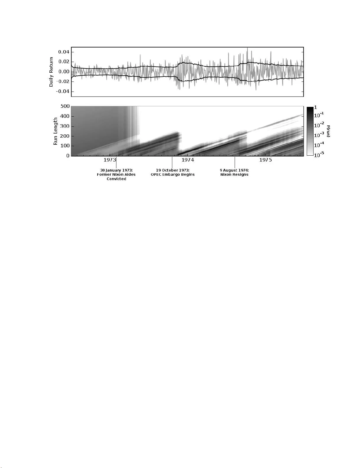
Ba y esian Online Changep oin t Detectio n Ry an Prescott A dams Cav endish Lab orator y Cambridge CB3 0HE United Kingdom Da vid J.C. Mac Kay Cav endish Lab orator y Cambridge CB3 0HE United Kingdom Abstract Changep oints are abrupt v ariations in the generative pa rameters of a data s e q uence. Online detection of c ha ngepo in ts is useful in mo delling and predictio n of time series in application a r eas such as finance, biomet- rics, and rob otics. While fr e q uen tist meth- o ds ha ve yielded online filtering and predic- tion techniques, mo st Bayesian pap ers hav e fo c us ed on the retrosp ective segmentation problem. Here we examine the case where the mo del parameters b e fore a nd after the changepoint ar e indep endent and we derive an online algorithm for exact inference of the most r ecent c ha ng epo in t. W e compute the probability distributi o n of the leng th of the current “r un,” or time since the last change- po in t, using a s imple message- pa ssing alg o - rithm. Our i mplementation is highly mo du- lar so that the a lgorithm may b e applied t o a v a riety o f types o f da ta. W e illustrate this mo dularity b y demonstrating the algorithm on three differen t r eal-world data sets. 1 INTRO DUCTI ON Changep oint detection is the identification o f abrupt changes in t he gener ative parameter s of s equent ia l data. As an online and offline s ig nal pro cessing too l, it has prov en to be useful in applicatio ns such a s pro ces s control [1 ], EEG analysis [5, 2, 17], DNA seg men tation [6], econometrics [7, 18], and disease demo graphics [9]. F requen tist approa c hes to c hang epo in t detection, from the pioneer ing work of Page [22, 23] and Lorden [19] to r ecent work using suppo rt vector machines [1 0], o f- fer o nline c hang epo in t detector s. Most Bayesian ap- proaches to changepo in t detection, in contrast, hav e been offline and r etrosp ective [24, 4, 26, 1 3, 8]. With a few exceptions [16, 20], the Bay esian paper s on change- po in t detection fo cus o n segmentation and tec hniques to g enerate sa mples from the po sterior dis tr ibution ov er changepoint lo cations. In this pap er, we present a Bayesian changep oint de- tection alg o rithm for online inference. Rather than retrosp ective segmentation, we fo cus on causal predic- tiv e filtering; genera ting an accur ate distribution o f the next unseen datum in the sequence, given o nly data al- ready o bserved. F or ma n y applications in ma c hine in- telligence, this is a natur a l requirement. Rob ots must navigate based on past sensor data from an environ- men t that may hav e a bruptly changed: a do o r may be clos e d now, for exa mple, or the furniture may have been mov ed. In vision systems, the brightn es s change when a lig h t switch is flipp ed o r when the sun comes out. W e assume that a sequence o f observ ations x 1 , x 2 , . . . , x T may b e divided into non-overlapping pr o duct p artitions [3 ]. The delineations betw een partitions are called the changep oints. W e further assume that for each partition ρ , the data within it are i.i.d. fro m some probability distribution P ( x t | η ρ ). The para meters η ρ , ρ = 1 , 2 , . . . are ta ken to be i.i.d. as w ell. W e deno te the contiguous set of observ ations betw een time a and b inclusive as x a : b . The discrete a priori probability distribution ov er the interv al betw een changepoints is deno ted as P gap ( g ). W e are concerned with es timating the po sterior dis- tribution ov er the cur rent “ run length,” or time since the last changepoint, given the data so far obser ved. W e denote the length of the cur r ent run at time t b y r t . W e also use the no tation x ( r ) t to indica te the set of o bserv ations a sso ciated with the run r t . As r may be zer o, the set x ( r ) may be empty . W e illustra te the relationship b etw een the r un length r and some hypo - thetical univ ariate data in Figures 1 (a ) and 1(b). x t g g g 1 2 3 (a) t r t 6 5 4 3 2 1 7 8 9 10 11 12 13 14 1 2 3 4 0 (b) r t 1 2 3 4 0 (c) Figure 1: This figure illustra tes how we describ e a changepoint mo del expressed in ter ms of run lengths. Figure 1(a) shows hypothetical univ aria te data divided b y c ha ngep o in ts on the mean into three segments of lengths g 1 = 4, g 2 = 6, a nd an undetermined length g 3 . Figure 1(b) shows the r un leng th r t as a function of time. r t drops to zero when a changep oint o ccurs . Figure 1(c) shows the trellis on which the mess age- passing algorithm liv es . Solid lines indicate that prob- abilit y mass is b eing pa ssed “upw ar ds,” causing the run length to grow at the next time step. Dotted lines indicate the p oss ibilit y that the current run is trun- cated and the run length drops to zero. 2 RECURSIVE RU N LENGTH ESTIMA TION W e assume that we can compute the predictive distri- bution conditional on a g iv en run length r t . W e then in teg r ate over the pos terior distribution o n the c ur rent run leng th to find the marginal pr edictiv e distribution: P ( x t +1 | x 1: t ) = X r t P ( x t +1 | r t , x ( r ) t ) P ( r t | x 1: t ) (1) T o find the po sterior distribution P ( r t | x 1: t ) = P ( r t , x 1: t ) P ( x 1: t ) , (2) we write the joint distribution ov er run length and observed data r ecursively . P ( r t , x 1: t ) = X r t − 1 P ( r t , r t − 1 , x 1: t ) = X r t − 1 P ( r t , x t | r t − 1 , x 1: t − 1 ) P ( r t − 1 , x 1: t − 1 ) (3) = X r t − 1 P ( r t | r t − 1 ) P ( x t | r t − 1 , x ( r ) t ) P ( r t − 1 , x 1: t − 1 ) Note that the predictive distribution P ( x t | r t − 1 , x 1: t ) depends only on the recent da ta x ( r ) t . W e can th us generate a r ecursive mess age-pass ing algor ithm for the joint distribution ov er the c ur rent r un leng th a nd the data, based on tw o ca lculations: 1) the prior ov er r t given r t − 1 , and 2) the predictive distribution ov er the newly-observed datum, g iv en the data since the las t changepoint. 2.1 THE CHANGEPOINT PRIOR The conditional prior on the changepoint P ( r t | r t − 1 ) gives this algorithm its computational efficiency , as it has nonzero mass at only tw o o utcomes: the run length either contin ues to g row and r t = r t − 1 + 1 or a c ha ng e- po in t o ccurs and r t = 0. P ( r t | r t − 1 ) =    H ( r t − 1 + 1) if r t = 0 1 − H ( r t − 1 + 1) if r t = r t − 1 + 1 0 otherwise (4) The function H ( τ ) is the hazar d funct ion . [11]. H ( τ ) = P gap ( g = τ ) P ∞ t = τ P gap ( g = t ) (5) In the sp ecial case is wher e P gap ( g ) is a discrete expo - nen tial (geometric) distribution with timescale λ , the pro cess is memoryless and the hazard function is co n- stant at H ( τ ) = 1 /λ . Figure 1 (c) illustra tes the resulting message- passing algorithm. In this diagr a m, the circles repres e nt r un- length hypothese s . The lines b et ween the circles show recursive transfer of mas s b etw een time steps. Solid lines indicate that probability mass is b eing passed “upw ards,” ca using the run le ng th to grow at the next time step. Dotted lines indica te that the current run is truncated and the run length drops to zero . 2.2 BOUNDAR Y CON DITIONS A recur s ive algo r ithm must not only define the re c ur- rence relation, but a lso the initialization conditions. W e co nsider tw o cases: 1) a changepoint o cc ur red a priori b efore the fir st datum, such as when observing a game. In such case s we plac e a ll of the probability mass for the initial run length a t zer o, i.e. P ( r 0 = 0 ) = 1. 2) W e obse r ve so me rece nt subset of the data, such as when mo delling climate change. In this case the prior ov er the initial r un length is the normalized su rvival function [11] P ( r 0 = τ ) = 1 Z S ( τ ) , (6) where Z is an appropr ia te nor malizing c o nstant, and S ( τ ) = ∞ X t = τ +1 P gap ( g = t ) . (7) 2.3 CON JUGA TE-EXPONENTIAL MODELS Conjugate-exp onential mo dels ar e particularly conv e- nien t for integrating with the changep oint detection scheme describ ed here. E xpo nen tial family likelihoo ds allow inference with a finite num b er of sufficient statis- tics which can b e calculated incrementally as data ar- rives. Exp onential family likelihoo ds hav e the form P ( x | η ) = h ( x ) exp ( η ⊺ U ( x ) − A ( η )) (8) where A ( η ) = log Z d η h ( x ) exp ( η ⊺ U ( x )) . (9) The str e ng th of the conjugate-ex p onential r epresenta- tion is that b oth the prior and p osterior take the for m of a n exp onential-family distr ibution over η that can be summar ize d by succinct hyper pa rameters ν and χ . P ( η | χ , ν ) = ˜ h ( η ) exp  η ⊺ χ − ν A ( η ) − ˜ A ( χ , ν )  (10) W e wish to infer the par ameter vector η asso ciated with the data fro m a current run length r t . W e denote this run-sp ecific mo del parameter as η ( r ) t . After find- ing the p o sterior distribution P ( η ( r ) t | r t , x ( r ) t ), we ca n marginalize out the pa rameters to find the pr e dictive distribution, conditional on the length of the current run. P ( x t +1 | r t ) = Z d η P ( x t +1 | η ) P ( η ( r ) t = η | r t , x ( r ) t ) (11) 1. Initialize P ( r 0 ) = ˜ S ( r ) or P ( r 0 = 0 ) = 1 ν (0) 1 = ν prio r χ (0) 1 = χ prio r 2. Observ e New Datum x t 3. Ev aluate Predi ctive Probabili t y π ( r ) t = P ( x t | ν ( r ) t , χ ( r ) t ) 4. Calculate Gro wth Probabilitie s P ( r t = r t − 1 + 1 , x 1: t ) = P ( r t − 1 , x 1: t − 1 ) π ( r ) t (1 − H ( r t − 1 )) 5. Calculate Changep oint Probabili ties P ( r t = 0 , x 1: t ) = X r t − 1 P ( r t − 1 , x 1: t − 1 ) π ( r ) t H ( r t − 1 ) 6. Calculate Evidence P ( x 1: t ) = X r t P ( r t , x 1: t ) 7. Determine Run Length Distribution P ( r t | x 1: t ) = P ( r t , x 1: t ) /P ( x 1: t ) 8. Up date Sufficie n t Statistics ν (0) t + 1 = ν prio r χ (0) t + 1 = χ prio r ν ( r + 1) t + 1 = ν ( r ) t + 1 χ ( r + 1) t + 1 = χ ( r ) t + u ( x t ) 9. P erform Prediction P ( x t + 1 | x 1: t ) = X r t P ( x t + 1 | x ( r ) t , r t ) P ( r t | x 1: t ) 10. Return to Step 2 Algorithm 1: The online changepoint algor ithm with prediction. An additional optimization not shown is to truncate the pe r -timestep vectors when the tail of P ( r t | x 1: t ) has ma ss b eneath a threshold. This mar ginal predictive distribution, while gener - ally not itself an exp onential-family distribution, is usually a simple function of the sufficient statistics. When ex act distributions are no t a v ailable, co mpa ct approximations such as that describ ed by Snelson and Ghahramani [2 5] may b e use ful. W e will only ad- dress the exact case in this pap er, where the pr edictiv e distribution asso ciated with a particular cur rent run length is pa rameterized by ν ( r ) t and χ ( r ) t . ν ( r ) t = ν prio r + r t (12) χ ( r ) t = χ prio r + X t ′ ∈ r t u ( x t ′ ) (13) Figure 2: The top plot is a 1100- datum subset of nuclear magnetic re s po nse during the drilling o f a well. The data ar e plotted in light gray , with the pr edictiv e mean (solid da rk line) and predictive 1- σ error bars (dotted lines) ov erla id. The b o ttom plot s hows the p osterior probability of the curr e n t run P ( r t | x 1: t ) at each time step, using a lo g arithmic color sca le. Darker pixels indicate higher proba bilit y . 2.4 COM PUT A TIONAL COST The co mplete a lgorithm, ass uming exp onential-family likelih o o ds, is shown in Algorithm 1 . The space- a nd time-complexity pe r time-step are linear in the n umber of da ta p oints so far obser ved. A trivial mo dification of the a lgorithm is to discard the r un length pro babilit y estimates in the tail o f the distribution which hav e a total mass less tha n some threshold, say 10 − 4 . This yields a consta n t av erag e complexity p er iteration o n the or der o f the exp ected run length E [ r ], although the worst-case co mplexit y is still linear in the data. 3 EXPERI MENT AL RESUL TS In this section we demons tr ate several implement a - tions o f the changep oint algor ithm developed in this pap er. W e examine three real- w o rld e x ample datasets. The first ca se is a v ar ying Gaussian mean from well- log data. In the second example we consider a br upt changes o f v ariance in daily returns o f the Dow Jones Industrial Average. The final data a re the interv als betw een co a l mining disasters, which we mo del as a Poisson pro cess. In each of the thre e ex a mples, we use a discrete exp onential prior ov er the int er v al b etw een changepoints. 3.1 WE LL-LOG D A T A These data ar e 405 0 measurements of n uclea r mag netic resp onse taken during the dr illing of a well. The data are use d to interpret the g eophysical str uctur e o f the ro ck surrounding the well. T he v aria tions in mean reflect the str a tification o f the earth’s crust. These data hav e b een studied in the context of changepoint detection by ´ O Ruanaidh and Fitzgerald [21], a nd by F e a rnhead and Cliffor d [12]. The changepo in t detection alg orithm was run o n these data using a univ a riate Gauss ian mo del with prio r pa- rameters µ = 1 . 15 × 10 5 and σ = 1 × 10 4 . The rate of the discre te exp onential prior, λ gap , was 25 0 . A sub- set of the data is shown in Figur e 2, with the predic- tiv e mean and standard deviation ov er la id on the top plot. The b ottom plot shows the log proba bility over the c urrent r un leng th a t e a ch time step. Notice that the drops to zer o r un-length cor resp ond w ell with the abrupt changes in the mean o f the data. Immediately after a changepo in t, the predictive v a r iance incr eases, as would b e exp ected for a sudden r eduction in data. 3.2 19 7 2-75 DO W JONES RETURNS During the three year p erio d fro m the middle of 1972 to the middle of 1 975, s everal ma jor even ts o ccurr ed that had po tential macro economic effects. Significant among these are the W atergate affair and the OPEC oil embargo. W e applied the changepo in t detection algorithm des crib ed here to daily returns of the Dow Jones Industrial Av er a ge from July 3, 1 9 72 to June 30 , 1975. W e mo delled the returns R t = p close t p close t − 1 − 1 , (14) Figure 3: The top plot shows daily returns on the Dow Jones Industrial Average, with an overlaid plot of the predictive volatilit y . The b ottom plot shows the p os terior probability of the c ur rent run leng th P ( r t | x 1: t ) at each time step, using a lo garithmic color scale. Darker pixels indicate higher probability . The time axis is in business days, as this is market data. Three even ts are ma rked: the conviction o f G. Gor don Liddy and Ja mes W. McCo rd, Jr. on J anuary 30, 1973 ; the b eginning of the OPE C em barg o against the United States on O c to ber 19, 19 73; and the r esignation of P resident Nixon on August 9, 19 74. (where p close is the daily closing price) with a zero- mean Ga ussian distribution and piecewise- constant v a r iance. Hsu [14] p erfor med a similar analysis on a subset of these data, using frequentist techniques and weekly returns. W e used a gamma prior on the in verse v ar iance, with a = 1 a nd b = 10 − 4 . The exp onential prior on change- po in t interv a l had rate λ gap = 250. In Figure 3, the top plot shows the daily r e tur ns with the predictive standard deviation overlaid. The b ottom plo t shows the p osterio r probability of the current r un length, P ( r t | x 1: t ). Three even ts ar e marked o n the plot: the conviction of Nixon re-election o fficials G. Gor don Liddy and Ja mes W. McCord, Jr ., the b eginning of the oil embargo against the United States by the Or- ganization of Petroleum Exp orting Countries (OPEC), and the r e signation of P r esident Nixon. 3.3 COAL MINE DISASTER D A T A These data fro m J arrett [15] are dates of coal mining explosions that killed ten or more men betw een March 15, 185 1 and March 22, 1962 . W e mo delled the da ta as an Poisson pro cess by weeks, with a g amma prior on the rate with a = b = 1. The rate o f the exp onen- tial prior on the changep oint inv erv al w a s λ gap = 10 00. The da ta are shown in Figure 4. The to p plot shows the cumulativ e num b er of accidents. The r ate o f the Possion pro cess determines the lo c a l av erage of the slop e. The p osterior probability o f the cur rent run length is shown in the b ottom plot. The introduc- tion o f the Co al Mines Regulations Act in 1887 (cor- resp onding to weeks 186 8 to 1920) is also marked. 4 DISCUSSION This pa per contributes a predictive, online interpeta- tion of Bay esia n changepoint detection and provides a simple a nd exact metho d fo r calculating the po ste- rior proba bilit y of the curre nt run length. W e hav e demonstrated this algor ithm o n thr e e r eal-world data sets with different mo delling r equirements. Additionally , this fr amework provides conv enient de- lineation b etw een the implementation of the ch a nge- po in t a lgorithm a nd the implementation of the mo del. This mo dularity allows changepo in t-detection co de to use an ob ject-o riented, “ pluggable” t yp e a rchit ec ture . Ac kno wledg emen ts The a uthors would like to thank Phil Cow ans and Mar- ian F razier for v aluable discussions. This work was funded by the Gates Ca m br idg e T rust. Figure 4: These da ta a re the weekly o ccurrence of coal mine disa sters that killed ten or mor e p eople b etw een 1851 and 1962. The top plot is the cumulativ e n umber o f accidents. The accident rate determines the lo cal av erag e slop e of the plot. The introduction of the Coal Mines Regulations Act in 1887 is mar ked. The year 1887 corresp onds to weeks 186 8 to 1920 on this plot. The b o ttom plot shows the p oster ior probability of the current run length a t each time step, P ( r t | x 1: t ). References [1] Leo A. Aro ian a nd How a rd Levene. The effec- tiv enes s of q ualit y control charts. Journal of the Ameri c an S tatistic al Ass o ciation , 45 (252):520 – 529, 195 0. [2] J. S. Ba r low, O. D. Cr eutzfeldt, D. Michael, J. Houchin , and H. Ep elbaum. Automatic adaptive seg men tation of clinical EEGs,. Ele c- tr o enc ephalo gr aphy and Clinic al Neur ophysiolo gy , 51(5):512 –525, May 19 81. [3] D. Barry and J . A. Hartiga n. Product partition mo dels fo r ch a nge p oint problems. The A nnals of Statistics , 20:26 0–279 , 1 992. [4] D. Barr y a nd J. A. Har tigan. A Bay esian analysis of change p oint problems. Journ al of the Ameri- c an Statistic al Asso ciation , 88:309 –319, 19 93. [5] G. Bo denstein and H. M. Pra etorius. F eature ex- traction from the e le c tr o encephalogram by adap- tiv e segment a tion. Pr o c e e dings of the IEEE , 65(5):642 –652, 1977 . [6] J. V. Braun, R. K. Br aun, and H. G. M ¨ uller. Multiple changepoint fitting via quasilikeliho o d, with application to DNA sequence seg men tation. Biometrika , 8 7 (2):301–3 14, June 200 0. [7] Jie Chen and A. K. Gupta. T esting and lo cating v a r iance changepoints with applica tion to sto ck prices. Journal of the Americ an St atistic al Asso- ciation , 92(4 38):739– 747, June 1997 . [8] Siddhartha Chib. Estimation and compariso n of m ultiple change-p oint mo dels. Journal of Ec ono- metrics , 86(2 ):2 21–24 1, Octob er 1998. [9] D. Denison and C. Holmes. Bay esian pa rtitioning for estimating disea se risk, 1 999. [10] F. Deso bry , M. Davy , and C . Donca rli. An on- line kernel change detection algorithm. IEEE T r ansactions on Signal Pr o c essing , 5 3(8):2961 – 2974, August 20 05. [11] Merra n Ev ans, Nicholas Hastings, and Br ian Peacock. Statistic al Distributions . Wiley- In ter science, J une 200 0. [12] Paul F ear nhead and Peter Clifford. On-line in- ference for hidden Markov mo dels via particle fil- ters. Journal of the R oyal Statistic al So ciety B , 65(4):887 –899, 2003 . [13] P . Green. Rev ers ible jump Marko v chain Monte Carlo computation and Bay esia n mo del determi- nation, 199 5 . [14] D. A. Hsu. T ests for v ar iance shift at an un- known time p oint. Applie d Statistics , 26 (3):279– 284, 197 7. [15] R. G. Jarrett. A no te on the interv als b etw een coal-mining disasters. Biometrika , 66(1):191 –193, 1979. [16] Timothy T. Jer vis and Stuart I. Jardine. Alarm system for wellbore site. United States Patent 5,952,5 69, Octob er 19 97. [17] A. Y. Kaplan a nd S. L. Shishkin. Application of the change-p oint analys is to the inv estigation of the brain’s electrical activity . In B. E. Bro dsky and B. S. Dar khovsky , editor s, Non-Par ametric Statistic al Diagnosis : Pr oblems and Metho ds , pages 333– 388. Springer , 2000. [18] Gary M. Ko o p and Simon M. Potter. F oreca st- ing a nd estimating multiple change-po in t mo dels with a n unknown n umber of change p oints. T ec h- nical rep ort, F ederal Reserve Bank of New Y ork, Decem b er 2 004. [19] G. Lo r den. Pr o cedures for rea cting to a change in distribution. The A nnals of Mathematic al Statis- tics , 42 (6 ):1897–1 908, December 1971 . [20] J. J. ´ O Ruanaidh, W. J. Fitzgera ld, a nd K. J. Pope. Recursive B ayesian lo cation of a discon- tin uity in time series. In A c oustics, Sp e e ch, and Signal Pr o c essing, 1994. ICASS P-94., 1994 IEEE International Confer enc e on , volume iv, pages IV/513– IV/516 vol.4, 1 994. [21] Joseph J. K. ´ O Ruana idh and William J . Fitzger - ald. Numeric al Bay esian Metho ds Applie d to Signal Pr o c essing (Statistics and Computing) . Springer, F ebruary 19 96. [22] E. S. Page. Contin uous inspectio n schem es . Biometrika , 4 1 (1/2):100 –115, June 195 4. [23] E. S. Page. A test for a change in a pa rame- ter o ccurring a t an unknown p oint. Biometrika , 42(3/4 ):5 23–52 7, 1955 . [24] A. F. M. Smith. A Bayesian approach to infer- ence a bo ut a change-p oint in a sequence of ran- dom v ariables. Biometrika , 62(2 ):407–41 6, 1975. [25] Edward Snelson and Zo ubin Ghahramani. Com- pact approximations to Bay esian predictive dis- tributions. In ICML ’05 : Pr o c e e dings of the 22nd international c onfer enc e on Machine le arn- ing , pa ges 84 0–847 , New Y o rk, NY, USA, 2 005. A CM P ress. [26] D. A. Stephens. Bay es ian r e trosp ective multipl e- changepoint iden tification. Applie d Statistics , 43:159 –178, 1994 .