On the Whitham Equations for the Defocusing Complex Modified KdV Equation

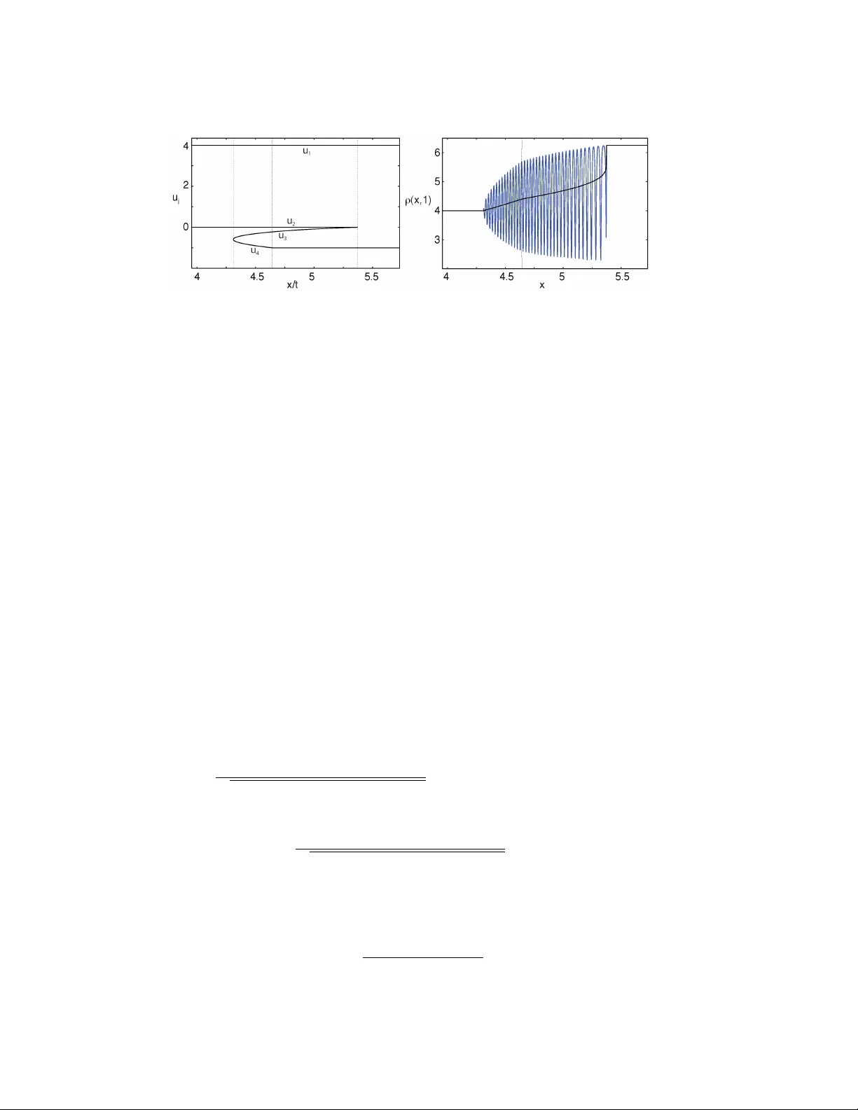
ON THE WHITHAM EQUA TIONS F OR THE DEF OCUSING COMPLEX MODIFIED KD V EQUA TION ∗ YUJI KOD AMA † , V. U. PIERCE ‡ , AND FEI-RAN TIAN § Abstract. W e study the Whitham equations for the defocusing complex modified KdV (mKdV) equation. These Whitham equations are quasilinear h yperb olic equations and they describ e the av eraged dynamics of the rapid oscillations which appear in the solution of the mKdV equation when the dispersive parameter is small. The oscillations are referred to as disp ersiv e shocks. The Whitham equations for the mKdV equation are neither strictly hyperb olic nor gen uinely nonlinear. W e are interested in the solutions of the Whitham equations when the initial v alues are given by a step function. W e also compare the results with those of the defo cusing nonlinear Sc hr¨ odinger (NLS) equation. F or the NLS equation, the Whitham equations are strictly hyperb olic and genuinely nonlinear. W e show that the weak hyperb olicit y of the mKdV-Whitham equations is resp onsible for an additional structure in the disp ersive sho cks which has not b een found in the NLS case. Key w ords. Whitham equations, non-strictly hyperb olic equations, disp ersiv e sho cks AMS sub ject classifications. 35L65, 35L67, 35Q05, 35Q15, 35Q53, 35Q58 1. In tro duction. In [11, 12], Pierce and Tian studied the self-similar solutions of the Whitham equations which describ e the zero disp ersion limits of the KdV hierarc hy . The main feature of the Whitham equations for the higher mem bers of the hierarc h y , of whic h the KdV equation is the first member, is that these Whitham equations are neither strictly hyperb olic nor gen uinely nonlinear. This is in sharp contrast to the case of the KdV equation whose Whitham equations are strictly h yperb olic and gen uinely nonlinear . In this pap er, we extend their studies to the case of the complex mo dified KdV equation, which is the second mem b er of the defo cusing nonlinear Sc hr¨ odinger hierarch y . The Whitham equations for the defo cusing NLS equation are strictly h yp erbolic and genuinely nonlinear, and they hav e b een studied extensively (see for examples, [4, 6, 7, 10, 13]). How ev er, for the mKdV equation, the Whitham equations are neither strictly hyperb olic nor genuinely nonlinear. Let us b egin with a brief description of the zero disp ersion limit of the solution of the NLS equation √ − 1  ∂ ψ ∂ t + 2  2 ∂ 2 ψ ∂ x 2 − 4 | ψ | 2 ψ = 0 , (1.1) with the initial data ψ ( x, 0) = A 0 ( x ) exp  √ − 1 S 0 ( x )   . Here A 0 ( x ) and S 0 ( x ) are real functions that are indep endent of  . W riting the solution ψ ( x, t ;  ) = A ( x, t ;  ) exp  √ − 1 S ( x,t ;  )   , and using the notation ρ ( x, t ;  ) = A 2 ( x, t ;  ), v ( x, t ;  ) = ∂ S ( x, t,  ) /∂ x , one obtains the conserv ation form of the defo cusing NLS equation      ∂ ρ ∂ t + ∂ ∂ x (4 ρv ) = 0 , ∂ ∂ t ( ρv ) + ∂ ∂ x  4 ρv 2 + 2 ρ 2  =  2 ∂ ∂ x  ρ ∂ 2 ∂ x 2 ln ρ  . (1.2) ∗ Department of Mathematics, Ohio State Universit y , 231 W. 18th Av enue † kodama@math.ohio-state.edu ‡ vpierce@math.ohio-state.edu § tian@math.ohio-state.edu 1 2 Y. KOD AMA, V.U. PIERCE AND F.-R. TIAN The mass density ρ = | ψ | 2 and momentum density ρv = √ − 1 2 ( ψ ψ ∗ x − ψ ∗ ψ x ) hav e w eak limits as  → 0 [6]. These limits satisfy a 2 × 2 system of hyperb olic equations      ∂ ρ ∂ t + ∂ ∂ x (4 ρv ) = 0 , ∂ ∂ t ( ρv ) + ∂ ∂ x  4 ρv 2 + 2 ρ 2  = 0 , (1.3) un til its solution dev elops a shock. System (1.3) can b e rewritten in the diagonal form for ρ 6 = 0, ∂ ∂ t  α β  + 2  3 α + β 0 0 α + 3 β  ∂ ∂ x  α β  = 0 , (1.4) where the Riemann inv ariants α and β are given b y α = v 2 + √ ρ , β = v 2 − √ ρ . (1.5) As a simple example, we consider the case with α = a =constant. System (1.4) reduces to a single equation ∂ β ∂ t + 2( a + 3 β ) ∂ β ∂ x = 0 . (1.6) The solution is given by the implicit form β ( x, t ) = f ( x − 2( a + 3 β ) t ) , where f ( x ) = β ( x, 0) is the initial data for β . One can easily see that if β ( x, 0) decreases in some region, then β ( x, t ) develops a sho c k in a finite time, i.e., ∂ β /∂ x b ecomes singular. After the sho c k formation in the solution of (1.3) or (1.4), the weak limits are describ ed b y the NLS-Whitham equations, which can also b e put in the Riemann in v ariant form [4, 6, 7, 10] ∂ u i ∂ t + λ g ,i ( u 1 , . . . , u 2 g +2 ) ∂ u i ∂ x = 0 , i = 1 , 2 , . . . , 2 g + 2 , (1.7) where λ g ,i are expressed in terms of complete h yp erelliptic integrals of genus g [8]. Here the n um b er g is exactly the num b er of phases in the NLS oscillations with small disp ersion. Accordingly , the zero phase g = 0 corresponds to no oscillations, and single and higher phases g ≥ 1 corresp ond to the NLS oscillations. System (1.4) is view ed as the zero phase Whitham equations. The solution of the Whitham equations (1.7) for g ≥ 1 then describ es the av eraged motion of the oscillations app earing in the solution of (1.1) (see e.g. [7]). Let us discuss the most imp ortan t g = 1 case in more detail. W e note that it is well known that the KdV oscillatory solution, in the single phase regime, can b e appro ximately describ ed b y the KdV p erio dic solution when the disp ersiv e parameter is small [1, 5, 16]. It is v ery possible to use the metho d of [1, 16] to show that the solution of the NLS equation (1.1) for small  can be approximately describ ed, in the single phase regime, by the p eriodic solution of the NLS equation. The NLS perio dic solution has the form ˜ ρ ( x, t ;  ) = ρ 3 + ( ρ 2 − ρ 3 ) sn 2 ( √ ρ 1 − ρ 3 θ ( x, t ;  ) , s ) . (1.8) WHITHAM EQUA TIONS FOR THE COMPLEX MODIFIED KDV 3 with θ ( x, t ;  ) = ( x − V 1 t ) / and the velocity V 1 = V 1 ( ρ 1 , ρ 2 , ρ 3 ). Here ρ i ’s are deter- mined b y the equation obtained from (1.2)  2 4  dρ dθ  2 = ( ρ − ρ 1 )( ρ − ρ 2 )( ρ − ρ 3 ) with ρ 1 > ρ 2 > ρ 3 , and sn( z , s ) is the Jacobi elliptic function with the mo dulus s = ( ρ 2 − ρ 3 ) / ( ρ 1 − ρ 3 ). W e can also write ρ i ’s as [3]            ρ 1 = 1 4 ( u 1 + u 2 − u 3 − u 4 ) 2 ρ 2 = 1 4 ( u 1 − u 2 + u 3 − u 4 ) 2 ρ 3 = 1 4 ( u 1 − u 2 − u 3 + u 4 ) 2 (1.9) with u 1 > u 2 > u 3 > u 4 . The velocity V 1 is then given by V 1 = 2( u 1 + u 2 + u 3 + u 4 ) . F or constants u 1 , u 2 , u 3 and u 4 , formula (1.8) gives the well kno wn elliptic solution of the NLS equation. T o describ e the solution ρ ( x, t ;  ) of the NLS equation (1.2), the quan tities u 1 , u 2 , u 3 and u 4 are instead functions of x and t and they evolv e according to the single phase Whitham equations (1.7) for g = 1. The w eak limit of ρ ( x, t ;  ) of NLS equation (1.1) as  → 0 can b e expressed in terms of ρ 1 , ρ 2 , ρ 3 and ρ 4 [6] ρ ( x, t ) = ρ 1 − ( ρ 1 − ρ 3 ) E ( s ) K ( s ) , (1.10) where K ( s ) and E ( s ) are the complete elliptic integrals of the first and second kind, resp ectiv ely . This weak limit can also b e view ed as the av erage v alue of the p eriodic solution ˜ ρ ( x, t ;  ) of (1.8) ov er its p eriod L = 2 K ( s ) / √ ρ 1 − ρ 3 . In order to see ho w a single phase Whitham solution app ears, w e consider the follo wing step initial data for system (1.4) α ( x, 0) = a, β ( x, 0) = ( b, x < 0 c, x > 0 , (1.11) where a > b , a > c , b 6 = c . The solution of (1.4) develops a sho ck if and only if b > c (cf. (1.6)). After the formation of a sho c k, the Whitham equations (1.7) with g = 1 kic k in. F or instance, we consider the Whitham equations with the initial data [7] u 1 ( x, 0) = a, u 2 ( x, 0) = b, u 3 ( x, 0) = ( b, x < 0 c, x > 0 , u 4 ( x, 0) = c. (1.12) No w notice that the Whitham equations (1.7) for g = 1 with the initial data (1.12) can b e reduced to a single equation u 3 t + λ 1 , 3 ( a, b, u 3 , c ) u 3 x = 0. The equation has a global self-similar solution, which is implicitly giv en b y x/t = λ 3 ( a, b, u 3 , c ). The x - t plane is then divided into thr e e parts (1) x t < γ , (2) γ < x t < 2 a + 4 b + 2 c , (3) x t > 2 a + 4 b + 2 c , where γ = 2( a + b + 2 c ) − 8( a − c )( b − c ) / ( a + b − 2 c ) (see (2.7) and (2.8) b elo w for the deriv ation). The solution of system (1.4) o ccupies the first and third parts, i.e., 4 Y. KOD AMA, V.U. PIERCE AND F.-R. TIAN (1) for x/t < γ , α ( x, t ) = a, β ( x, t ) = b, (3) for x/t > 2 a + 4 b + 2 c , α ( x, t ) = a, β ( x, t ) = c . The Whitham solution of (1.7) with g = 1 lives in the second part, i.e., (2) for γ < x/t < 2 a + 4 b + 2 c , u 1 ( x, t ) = a , u 2 ( x, t ) = b , x t = λ 1 , 3 ( a, b, u 3 , c ) , u 4 ( x, t ) = c , where the solution u 3 can b e obtained as a function of the self-similarity v ariable x/t , if ∂ λ 1 , 3 ∂ u 3 ( a, b, u 3 , c ) 6 = 0 . Indeed, it has been shown that the Whitham equations (1.7) are genuinely nonlinear [6, 7], i.e., ∂ λ 1 ,i ∂ u i ( u 1 , u 2 , u 3 , u 4 ) > 0 , i = 1 , 2 , 3 , 4 , (1.13) for u 1 > u 2 > u 3 > u 4 . In Figure 1, w e plot the self-similar solution of the Whitham equations (1.7) with g = 1 for the NLS equation, and the corresp onding p erio dic oscillatory solution (1.8) for the initial data (1.11) with a = 4 , b = 0 and c = − 1. The oscillations describ e a disp ersiv e sho c k of the NLS equation under a small dispersion. Note here that the oscillations hav e a uniform structure, whic h is due to an almost linear profile of the Whitham solution u 3 . This will b e seen to b e in sharp con trast to the case of the mKdV equation, which w e will discuss later (cf. Figure 1.2). Fig. 1.1 . Self-Similar solution of the NLS-Whitham e quation (1.7) of g = 1 and the corr e- sp onding oscil latory solution (1.8) of the NLS e quation with  = 0 . 15 . The dark line in the midd le of the oscil lations is the we ak limit ρ ( x, t ) given by (1.10). The initial data is given by (1.11) with a = 4 , b = 0 and c = − 1 . The figures in this pap er all hav e the same form: On the left hand side is a plot of the solution of the Whitham equations as a function of the self-similarity v ariable x/t , which is exact, other than a numerical metho d used to implement the inv erse function theorem. On the right hand side is the oscillatory solution given by (1.8) (resp ectiv ely (1.21) for mKdV) at t = 1, while the dark plot is the weak limit (1.10) WHITHAM EQUA TIONS FOR THE COMPLEX MODIFIED KDV 5 of the oscillatory solution at t = 1, both plots on the right are also exact. In the first tw o figures we demark the region where the Whitham equations with g = 1 go vern the solution, place a dashed-dotted line where the b ehavior of the oscillatory solution c hanges, and lab el the four functions u 1 > u 2 > u 3 > u 4 . The demarcation and labeling are similar in the other figures and we will leav e them off for brevit y . Although we do not include any n umerical sim ulations, we w ould like to men tion that E. Overman sho w ed us his numerical simulation of the NLS and mKdV equations whic h captures the features of the oscillatory solutions plotted in this pap er. The defo cusing NLS equation is just the first member of the defo cusing NLS hierarc hy; the second is the (defo cusing) complex modified KdV (mKdV) equation ∂ ψ ∂ t + 3 2 | ψ | 2 ∂ ψ ∂ x −  2 4 ∂ 3 ψ ∂ x 3 = 0 . (1.14) W e again use ψ ( x, t ;  ) = A ( x, t ;  ) exp  √ − 1 S ( x,t ;  )   and notation ρ ( x, t ;  ) = A 2 ( x, t ;  ), v ( x, t ;  ) = ∂ S ( x, t ;  ) /∂ x to obtain the conserv ation form of the mKdV equation        ∂ ρ ∂ t + ∂ ∂ x  3 4 ρ 2 + 3 4 ρv 2  =  2 ∂ ∂ x  ρ 3 / 4 ∂ 2 ∂ x 2 ρ 1 / 4  , ∂ ∂ t ( ρv ) + ∂ ∂ x  3 2 ρ 2 v + 3 4 ρv 3  =  2 4 ∂ ∂ x  ∂ 2 ∂ x 2 ( ρv ) − 3 2 R  , (1.15) where R = 3 v 2 ρ  ∂ ρ ∂ x  2 + ∂ v ∂ x ∂ ρ ∂ x − v ∂ 2 ρ ∂ x 2 . The mass density ρ and momentum density ρv for the mKdV equation also hav e w eak limits as  → 0 [6]. As in the NLS case, the w eak limits satisfy        ∂ ∂ t ρ + ∂ ∂ x  3 4 ρ 2 + 3 4 ρv 2  = 0 , ∂ ∂ t ( ρv ) + ∂ ∂ x  3 2 ρ 2 v + 3 4 ρv 3  = 0 , (1.16) un til the solution of (1.16) forms a sho ck. One can rewrite equations (1.16) as ∂ ∂ t  α β  + 3 8  5 α 2 + 2 αβ + β 2 0 0 α 2 + 2 αβ + 5 β 2  ∂ ∂ x  α β  = 0 , (1.17) where the Riemann inv ariants α and β are again given b y form ula (1.5). Let us again consider the simplest case α ( x, 0) = a , where a is constan t, to see ho w the solution of system (1.17) develops a sho ck. In this case, the system reduces to a single equation ∂ β ∂ t + 3 8  a 2 + 2 aβ + 5 β 2  ∂ β ∂ x = 0 . As in the NLS c ase, we consider the initial function given b y β ( x, 0) = b for x < 0 and β ( x, 0) = c for x > 0. W e recall that, in the NLS case, the zero phase solution of (1.4) develops a sho ck if and only if b > c . How ever, the solution in the mKdV case dev elops a shock for b > c if and only if a + 5 b > 0. In addition, if b < c , the solution 6 Y. KOD AMA, V.U. PIERCE AND F.-R. TIAN in the mKdV case develop a shock if and only if a + 5 b < 0. These differences b etw een the mKdV and NLS cases are due to the w eak h yp erb olicit y of the system (1.17) (note that for the eigensp eed λ = 3 8 ( α 2 + 2 αβ + 5 β 2 ) for β , we hav e ∂ λ/∂ β = 3 4 ( α + 5 β ) whic h can change sign). As will be sho wn b elow, this leads to an additional structure in the disp ersiv e sho c k for the mKdV case. As in the case of the NLS equation, immediately after the shock formation in the solution of (1.16), the weak limits are described by the mKdV-Whitham equations ∂ u i ∂ t + µ g ,i ( u 1 , . . . , u 2 g +2 ) ∂ u i ∂ x = 0 , i = 1 , 2 , 3 . . . , 2 g + 2 , (1.18) where µ g ,i ’s can also be expressed in terms of complete h yp erelliptic in tegrals of gen us g [6]. In this paper, we study the solution of the Whitham equations (1.18) with g = 1 when the initial mass density ρ ( x, 0) and momen tum density ρ ( x, 0) v ( x, 0) are step functions. In view of (1.5), this amounts to requiring α and β of system (1.17) to ha ve step-like initial data. W e are interested in the following t wo cases: (i) α ( x, 0) is a constant and α ( x, 0) = a , β ( x, 0) =  b, x < 0 c, x > 0 , a > b , a > c , b 6 = c , (1.19) (ii) β ( x, 0) is a constan t and α ( x, 0) =  b, x < 0 c, x > 0 , β ( x, 0) = a , b > a , c > a , b 6 = c . (1.20) In the case of the NLS equation, the genuine nonlinearity of the single phase Whitham equations (see (1.13)) w arran ts that the solution is found b y the implicit function theorem. How ever the mKdV-Whitham equations (1.18), in general, are not gen uinely nonlinear, that is, a property like (1.13) is not a v ailable (see Lemma 2.1 b elo w). Our construction of solutions of the Whitham equation (1.18) with g = 1 mak es use of the non-strict h yp erbolicity of the equations. F or the NLS case, it has b een known in [6, 7] that the Whitham equations (1.7) with g = 1 are strictly h yp erbolic, that is, λ 1 , 1 > λ 1 , 2 > λ 1 , 3 > λ 1 , 4 for u 1 > u 2 > u 3 > u 4 . F or the mKdV-Whitham equations (1.18) with g = 1, the eigensp eeds µ 1 ,i ( u 1 , u 2 , u 3 , u 4 ) ma y coale sce in the region u 1 > u 2 > u 3 > u 4 (w e will discuss the details in Section 2). Let us no w describ e one of our main results (see Theorem 3.1) for the single phase mKdV-Whitham equations with step-like initial function (1.19) for a = 4, b = 1 and c = − 1. In this case, the space time is divided into four regions (see Figure 1.2) instead of thr e e in the case of the NLS equation (cf. Figure 1) (1) x t < c 1 , (2) c 1 < x t < c 2 , (3) c 2 < x t < c 3 , (4) x t > c 3 , where c 1 , c 2 and c 3 are some constants. In the first and fourth regions, the solution of the 2 × 2 system (1.17) gov erns the ev olution: (1) for x/t < c 1 , α ( x, t ) = 4 , β ( x, t ) = 1 , WHITHAM EQUA TIONS FOR THE COMPLEX MODIFIED KDV 7 (4) for x/t > c 2 , α ( x, t ) = 4 , β ( x, t ) = − 1 . The Whitham solution of the 4 × 4 system (1.18) with g = 1 lives in the second and third regions; (2) for c 1 < x/t < c 2 , u 1 ( x, t ) = 4 , u 2 ( x, t ) = 1 , x t = µ 1 , 3 (4 , 1 , u 3 , u 4 ) , x t = µ 1 , 4 (4 , 1 , u 3 , u 4 ) , (3) for c 2 < x/t < c 3 , u 1 ( x, t ) = 4 , u 2 ( x, t ) = 1 , x t = µ 1 , 3 (4 , 1 , u 3 , − 1) , u 4 ( x, t ) = − 1 . Note that, in the second region, we ha v e µ 1 , 3 (4 , 1 , u 3 , u 4 ) = µ 1 , 4 (4 , 1 , u 3 , u 4 ) on a curve in the region − 1 < u 4 < u 3 < 4. This implies the non-strict h yp erbolicity of the mKdV-Whitham equations (1.18) for g = 1. It is again p ossible to use the metho d of [1, 16] to show that the solution of the mKdV equation (1.14) can be appro ximately describ ed, in the single phase regime, b y the p eriodic solution of the mKdV when  is small. The p eriodic solution has the same form as (1.8) of the NLS, i.e., ˜ ρ ( x, t ;  ) = ρ 3 + ( ρ 2 − ρ 3 ) sn 2 ( √ ρ 1 − ρ 3 θ ( x, t ;  ) , s ) . (1.21) Ho wev er, θ ( x, t ;  ) is now giv en by θ = ( x − V 2 t ) / with the velocity V 2 (see e.g. [9]) V 2 = 3 8 σ 2 1 − 1 2 σ 2 , where σ 1 = P 4 j =1 u j and σ 2 = P i b > c . In Section 4, we will construct the self-similar solution of the Whitham equations for the initial function (1.19) with a > c > b . In Section 5, we will briefly discuss how to handle the other step-like initial data (1.20). 2. The Whitham Equations. In this section we define the eigensp eeds λ g ,i ’s and µ g ,i ’s of the Whitham equations (1.7) and (1.18) with g = 1 for the NLS and the mKdV equations. F or simplicity , w e suppress the subscript g = 1 in the notation λ g ,i ’s and µ g ,i ’s in the rest of the pap er. W e first introduce the p olynomials of ξ for n = 0 , 1 , 2 , . . . [2, 4, 10]: P n ( ξ , u 1 , u 2 , u 3 , u 4 ) = ξ n +2 + a n, 1 ξ n + · · · + a n,n +2 , (2.1) where the co efficients, a n, 1 , a n, 2 , . . . , a n,n +2 are uniquely determined by the tw o con- ditions P n ( ξ , u 1 , u 2 , u 3 , u 4 ) p ( ξ − u 1 )( ξ − u 2 )( ξ − u 3 )( ξ − u 4 ) = ξ n + O ( ξ − 2 ) for large | ξ | and Z u 1 u 2 P n ( ξ , u 1 , u 2 , u 3 , u 4 ) p ( u 1 − ξ )( ξ − u 2 )( ξ − u 3 )( ξ − u 4 ) dξ = 0 . The co efficien ts of P n can b e expressed in terms of complete elliptic integrals. The eigensp eeds of the Whitham equations (1.7) with g = 1 for the NLS equation are defined in terms of P 0 and P 1 of (2.1) [4, 6, 10], λ i ( u 1 , u 2 , u 3 , u 4 ) = 8 P 1 ( u i , u 1 , u 2 , u 3 , u 4 ) P 0 ( u i , u 1 , u 2 , u 3 , u 4 ) , i = 1 , 2 , 3 , 4 , WHITHAM EQUA TIONS FOR THE COMPLEX MODIFIED KDV 9 whic h give λ i ( u 1 , u 2 , u 3 , u 4 ) = 2  σ 1 ( u 1 , u 2 , u 3 , u 4 ) − I ( u 1 , u 2 , u 3 , u 4 ) ∂ u i I ( u 1 , u 2 , u 3 , u 4 )  . (2.2) Here σ 1 := P 4 j =1 u j , and I ( u 1 , u 2 , u 3 , u 4 ) is given by a complete elliptic integral [13] I ( u 1 , u 2 , u 3 , u 4 ) = Z u 1 u 2 dη p ( u 1 − η )( η − u 2 )( η − u 3 )( η − u 4 ) . (2.3) The function I can be rewritten as a contour integral. Hence, 2( u i − u j ) ∂ 2 I ∂ u i ∂ u j = ∂ I ∂ u i − ∂ I ∂ u j , i, j = 1 , 2 , 3 , 4 (2.4) since the integrand satisfies the same equations for each η 6 = u i . This contour in tegral connection also allows us to giv e another formulation of I I ( u 1 , u 2 , u 3 , u 4 ) = Z u 3 u 4 dη p ( u 1 − η )( u 2 − η )( u 3 − η )( η − u 4 ) . (2.5) It follo ws from (2.2), (2.3) and (2.5) that λ 4 − 2 σ 1 < λ 3 − 2 σ 1 < 0 < λ 2 − 2 σ 1 < λ 1 − 2 σ 1 (2.6) for u 4 < u 3 < u 2 < u 1 . This implies the strict h yp erbolicity of the NLS-Whitham equation (1.7) for g = 1. The eigensp eeds λ i ’s ha ve the following v alues [13]: A t u 3 = u 4 , we hav e    λ 1 = 6 u 1 + 2 u 2 , λ 2 = 2 u 1 + 6 u 2 , λ 3 = λ 4 = 2( u 1 + u 2 + 2 u 4 ) − 8( u 1 − u 4 )( u 2 − u 4 ) u 1 + u 2 − 2 u 4 , (2.7) and at u 2 = u 3 ,    λ 1 = 6 u 1 + 2 u 4 , λ 2 = λ 3 = 2 u 1 + 4 u 3 + 2 u 4 , λ 4 = 2 u 1 + 6 u 4 . (2.8) Notice that the eigensp eed λ 2 = λ 3 at u 2 = u 3 is the same as the velocity of the p eriodic solution (1.8), i.e. V 1 = 2 σ 1 = 2( u 1 + 2 u 3 + u 4 ). The eigensp eeds of the mKdV-Whitham equations (1.18) with g = 1 are [6] µ i ( u 1 , u 2 , u 3 , u 4 ) = 3 P 2 ( u i , u 1 , u 2 , u 3 , u 4 ) P 0 ( u i , u 1 , u 2 , u 3 , u 4 ) , i = 1 , 2 , 3 , 4 . (2.9) They can b e expressed in terms of λ 1 , λ 2 , λ 3 and λ 4 of the NLS-Whitham equations (1.7) with g = 1. Lemma 2.1. The eigensp e e ds µ i ( u 1 , u 2 , u 3 , u 4 ) ’s of (2.9) c an b e expr esse d in the form µ i = 1 2 ( λ i − 2 σ 1 ) ∂ q ∂ u i + q , i = 1 , 2 , 3 , 4 , (2.10) 10 Y. KODAMA, V.U. PIERCE AND F.-R. TIAN wher e σ 1 = P 4 j =1 u j and q = q ( u 1 , u 2 , u 3 , u 4 ) is the solution of the b oundary value pr oblem of the Euler-Poisson-Darb oux e quations 2( u i − u j ) ∂ 2 q ∂ u i ∂ u j = ∂ q ∂ u i − ∂ q ∂ u j , i, j = 1 , 2 , 3 , 4 , (2.11) q ( u, u, u ) = 3 u 2 . A lso the µ i ’s satisfy the over-determine d systems 1 µ i − µ j ∂ µ i ∂ u j = 1 λ i − λ j ∂ λ i ∂ u j , i 6 = j . (2.12) W e omit the pro of since it is very similar to the pro of of an analogous result for the KdV hierarch y [14]. The b oundary v alue problem (2.11) has a unique solution. The solution is a symmetric quadratic function of u 1 , u 2 , u 3 and u 4 q = 3 8 σ 2 1 − 1 2 σ 2 , (2.13) where σ 2 = P i>j u i u j is the elemen tary symmetric p olynomial of degree t wo. Notice that q gives the velocity of the p eriodic solution (1.21) for the mKdV equation, i.e. V 2 = q . F or NLS, λ i ’s satisfy [13] ∂ λ 4 ∂ u 4 < 3 2 λ 3 − λ 4 u 3 − u 4 < ∂ λ 3 ∂ u 3 (2.14) for u 4 < u 3 < u 2 < u 1 . Similar results also hold for the mKdV-Whitham equations (1.18) with g = 1. Lemma 2.2. ∂ µ 3 ∂ u 3 > 3 2 µ 3 − µ 4 u 3 − u 4 if ∂ q ∂ u 3 > 0 , (2.15) ∂ µ 4 ∂ u 4 < 3 2 µ 3 − µ 4 u 3 − u 4 if ∂ q ∂ u 4 > 0 , (2.16) for u 4 < u 3 < u 2 < u 1 . Pr o of . W e use (2.10) and (2.14) to obtain ∂ µ 3 ∂ u 3 = 1 2 ∂ λ 3 ∂ u 3 ∂ q ∂ u 3 + 1 2 ( λ 3 − 2 σ 1 ) ∂ 2 q ∂ u 2 3 > 3 4 λ 3 − λ 4 u 3 − u 4 ∂ q ∂ u 3 + 1 2 ( λ 4 − 2 σ 1 ) ∂ 2 q ∂ u 2 3 , (2.17) and µ 3 − µ 4 = 1 2 ( λ 3 − λ 4 ) ∂ q ∂ u 3 + 1 2 ( λ 4 − 2 σ 1 )  ∂ q ∂ u 3 − ∂ q ∂ u 4  = 1 2 ( λ 3 − λ 4 ) ∂ q ∂ u 3 + ( λ 4 − 2 σ 1 )( u 3 − u 4 ) ∂ 2 q ∂ u 3 ∂ u 4 = 2 3 ( u 3 − u 4 )  3 4 λ 3 − λ 4 u 2 − u 3 ∂ q ∂ u 3 + 3 2 ( λ 4 − 2 σ 1 ) ∂ 2 q ∂ u 3 ∂ u 4  , (2.18) WHITHAM EQUA TIONS FOR THE COMPLEX MODIFIED KDV 11 where we hav e used equation (2.11) ∂ q ∂ u 3 − ∂ q ∂ u 4 = 2( u 3 − u 4 ) ∂ 2 q ∂ u 3 ∂ u 4 . It follo ws from formula (2.13) for q that 3 ∂ 2 q ∂ u 3 ∂ u 4 = ∂ 2 q ∂ u 2 3 , whic h, along with with (2.17) and (2.18), pro v es (2.15). Inequalit y (2.16) is pro v ed in the same wa y . The following calculations are useful in the subsequent sections. Using formula (2.10) for µ 3 and µ 4 and form ulae (2.2) for λ 3 and λ 4 , we obtain µ 3 − µ 4 = I ( ∂ u 3 I )( ∂ u 4 I )  ∂ q ∂ u 4 ∂ I ∂ u 3 − ∂ q ∂ u 3 ∂ I ∂ u 4  = I ( ∂ u 3 I )( ∂ u 4 I )  ∂ q ∂ u 4 ( ∂ I ∂ u 3 − ∂ I ∂ u 4 ) − ( ∂ q ∂ u 3 − ∂ q ∂ u 4 ) ∂ I ∂ u 4  = 2 I ( u 3 − u 4 ) ( ∂ u 3 I )( ∂ u 4 I ) M , (2.19) where M = ∂ q ∂ u 4 ∂ 2 I ∂ u 3 ∂ u 4 − ∂ 2 q ∂ u 3 ∂ u 4 ∂ I ∂ u 4 . Here w e ha v e used equations (2.4) for I and equations (2.11) for q in equalit y (2.19). Since q of (2.13) is quadratic, w e obtain ∂ M ∂ u 3 = ∂ q ∂ u 4 ∂ 3 I ∂ u 2 3 ∂ u 4 . (2.20) W e note that another expression for M is M = ∂ q ∂ u 3 ∂ 2 I ∂ u 3 ∂ u 4 − ∂ 2 q ∂ u 3 ∂ u 4 ∂ I ∂ u 3 . Hence, we get ∂ M ∂ u 4 = ∂ q ∂ u 3 ∂ 3 I ∂ u 3 ∂ u 2 4 . (2.21) W e next ev aluate M ( u 1 , u 2 , u 3 , u 4 ) when u 3 = u 4 . Using the integral form ula (2.3) for the function I and applying the change of v ariable η = ( u 1 − u 2 ) ν + u 2 , we obtain M    u 3 = u 4 = ∂ q ∂ u 4 4( u 2 − u 4 ) 3 Z 1 0 dν (1 + u 1 − u 2 u 2 − u 4 ν ) 3 p ν (1 − ν ) − ∂ 2 q ∂ u 3 ∂ u 4 2( u 2 − u 4 ) 2 Z 1 0 dν (1 + u 1 − u 2 u 2 − u 4 ν ) 2 p ν (1 − ν ) . 12 Y. KODAMA, V.U. PIERCE AND F.-R. TIAN The tw o integrals can be ev aluated exactly as Z 1 0 dν (1 + γ ν ) 3 p ν (1 − ν ) = π (8 + 8 γ + 3 γ 2 ) 8(1 + γ ) 5 2 , Z 1 0 dν (1 + γ ν ) 2 p ν (1 − ν ) = π (2 + γ ) 2(1 + γ ) 3 2 for γ > − 1. W e finally get M    u 3 = u 4 = π U ( u 1 , u 2 , u 4 ) 128[( u 2 − u 4 )( u 1 − u 4 )] 5 2 , (2.22) where U ( u 1 , u 2 , ξ ) = [8( u 2 − ξ ) 2 + 8( u 2 − ξ )( u 1 − u 2 ) + 3( u 1 − u 2 ) 2 ]( u 1 + u 2 + 4 ξ ) − 8( u 2 − ξ )[2( u 2 − ξ ) 2 + 3( u 2 − ξ )( u 1 − u 2 ) +( u 1 − u 2 ) 2 ] . (2.23) Similar to (2.19) for µ 3 and µ 4 , we hav e µ 2 − µ 3 = 2 I ( u 2 − u 3 ) ( ∂ u 2 I )( ∂ u 3 I ) N , (2.24) where N = ∂ q ∂ u 2 ∂ 2 I ∂ u 2 ∂ u 3 − ∂ 2 q ∂ u 2 ∂ u 3 ∂ I ∂ u 2 . Since q of (2.13) is quadratic, w e obtain ∂ N ∂ u 3 = ∂ q ∂ u 2 ∂ 3 I ∂ u 2 ∂ u 2 3 . (2.25) Finally , we use (2.7) and (2.10) to calculate ( µ 2 − µ 3 )    u 3 = u 4 = 1 2 [ λ 2 − 2( u 1 + u 2 + 2 u 4 )] ∂ q ∂ u 2 − 1 2 [ λ 3 − 2( u 1 + u 2 + 2 u 4 )] ∂ q ∂ u 3 = ( u 2 − u 4 ) 2( u 1 + u 2 − 2 u 4 ) V ( u 1 , u 2 , u 4 ) , (2.26) where V ( u 1 , u 2 , u 4 ) = 3 u 2 1 + 3 u 2 2 − 12 u 2 4 + 6 u 1 u 2 + 6 u 1 u 4 − 6 u 2 u 4 . (2.27) 3. Self-Similar Solutions. In this section, w e construct self-similar solutions of the Whitham equations (1.18) with g = 1 for the initial function (1.19) with a > b > c . The case with a > c > b will b e studied in next section. The solution of the zero phase Whitham equations (1.17) do es not develop a sho ck when a + 5 b ≤ 0. W e are therefore only interested in the case a + 5 b > 0. W e first study the ξ -zero of the cubic p olynomial equation U ( a, b, ξ ) = 0 , (3.1) where U is given by (2.23). It is easy to pro v e that for eac h pair of a and b satisfying a > b and a + 5 b > 0, U ( a, b, ξ ) = 0 has only one simple real root. Denoting this zero WHITHAM EQUA TIONS FOR THE COMPLEX MODIFIED KDV 13 b y ξ ( a, b ), we then deduce that U ( a, b, ξ ) is p ositive for ξ > ξ ( a, b ) and negativ e for ξ < ξ ( a, b ). Since U ( a, b, − ( a + b ) / 4) < 0 in view of (2.23), we m ust ha ve ξ ( a, b ) > − a + b 4 . (3.2) F or initial function (1.19) with a > b > c and a + 5 b > 0, we no w classify the resulting Whitham solutions into four types: (I) ξ ( a, b ) ≤ c with any a > b > c (I I) ξ ( a, b ) > c with a + 5 b > 3( b − c ) > 0 (I II) ξ ( a, b ) > c with a + 5 b = 3( b − c ) > 0 (IV) ξ ( a, b ) > c with 0 < a + 5 b < 3( b − c ) W e will study the second t yp e (II) first. 3.1. T yp e I I. Here we consider the step initial function (1.19) satisfying ξ ( a, b ) > c and a + 5 b > 3( b − c ) > 0. Theorem 3.1. (se e Figur e 1.2.) F or the step-like initial data (1.19) with a > b > c , a + 5 b > 3( b − c ) and ξ ( a, b ) > c , the solution ( α, β ) of the zer o phase Whitham e quations (1.17) and the solution ( u 1 , u 2 , u 3 , u 4 ) of the single phase Whitham e quations (1.18) with g = 1 ar e given as fol lows: (1) F or x/t ≤ µ 3 ( a, b, ξ ( a, b ) , ξ ( a, b )) , α = a , β = b . (3.3) (2) F or µ 3 ( a, b, ξ ( a, b ) , ξ ( a, b )) < x/t < µ 3 ( a, b, u ∗∗ , c ) , u 1 = a , u 2 = b , x t = µ 3 ( a, b, u 3 , u 4 ) , x t = µ 4 ( a, b, u 3 , u 4 ) , (3.4) wher e u ∗∗ is the unique solution u 3 of µ 3 ( a, b, u 3 , c ) = µ 4 ( a, b, u 3 , c ) in the interval c < u 3 < b . (3) F or µ 3 ( a, b, u ∗∗ , c ) ≤ x/t < µ 3 ( a, b, b, c ) , u 1 = a , u 2 = b , x t = µ 3 ( a, b, u 3 , c ) , u 4 = c. (3.5) (4) F or x/t ≥ µ 3 ( a, b, b, c ) , α = a , β = c. (3.6) The b oundaries x/t = µ 3 ( a, b, ξ ( a, b ) , ξ ( a, b )) and x/t = µ 3 ( a, b, b, c ) are called the trailing and leading edges, resp ectiv ely . They separate the solutions of the single phase Whitham equations (1.18) with g = 1 and the zero phase Whitham equations (1.17). The single phase Whitham solution matches the zero phase Whitham solution in the following fashion (see Figure 1.): ( u 1 , u 2 ) = the solution ( α, β ) of (1.17) defined outside the region , (3.7) u 3 = u 4 , (3.8) at the trailing edge; ( u 1 , u 4 ) = the solution ( α, β ) of (1.17) defined outside the region , (3.9) u 2 = u 3 , (3.10) 14 Y. KODAMA, V.U. PIERCE AND F.-R. TIAN at the leading edge. The pro of of Theorem 3.1 is based on a series of lemmas: W e first show that the solutions defined by formulae (3.4) and (3.5) indeed satisfy the Whitham equations (1.18) for g = 1 [2, 15]. Lemma 3.2. (1) The functions u 1 , u 2 , u 3 and u 4 determine d by e quations (3.4) give a solution of the Whitham e quations (1.18) with g = 1 as long as u 3 and u 4 c an b e solve d fr om (3.4) as functions of x and t . (2) The functions u 1 , u 2 , u 3 and u 4 determine d by e quations (3.5) give a solution of the Whitham e quations (1.18) with g = 1 as long as u 3 c an b e solve d fr om (3.5) as a function of x and t . Pr o of . (1) u 1 and u 2 ob viously satisfy the first tw o equations of (1.18) for g = 1. T o verify the third and fourth equations, we observe that ∂ µ 3 ∂ u 4 = ∂ µ 4 ∂ u 3 = 0 (3.11) on the solution of (3.4). T o see this, we use (2.12) to calculate ∂ µ 3 ∂ u 4 = ∂ λ 3 ∂ u 4 λ 3 − λ 4 ( µ 3 − µ 4 ) = 0 . The second part of (3.11) can b e shown in the same w ay . W e then calculate the partial deriv atives of the third equation of (3.4) with resp ect to x and t 1 = ∂ µ 3 ∂ u 3 tu 3 x , 0 = ∂ µ 3 ∂ u 3 tu 3 t + µ 3 , whic h give the third equation of (1.18) with g = 1. The fourth equation of (1.18) with g = 1 can b e v erified in the same wa y . (2) The second part of Lemma 3.2 can easily b e pro v ed. W e now determine the trailing edge. Eliminating x and t from the last tw o equations of (3.4) yields µ 3 ( a, b, u 3 , u 4 ) − µ 4 ( a, b, u 3 , u 4 ) = 0 . (3.12) Since it degenerates at u 3 = u 4 , we replace (3.12) by F ( a, b, u 3 , u 4 ) := µ 3 ( a, b, u 3 , u 4 ) − µ 4 ( a, b, u 3 , u 4 ) u 3 − u 4 = 0 . (3.13) Therefore, at the trailing edge where u 3 = u 4 , equation (3.13), in view of form ulae (2.19) and (2.22), reduces to U ( a, b, u 4 ) = 0 . (3.14) Noting that ξ ( a, b ) is the unique solution of (3.1), we then deduce that u 4 = ξ ( a, b ). Lemma 3.3. Equation (3.13) has a unique solution satisfying u 3 = u 4 . The solution is u 3 = u 4 = ξ ( a, b ) . The r est of e quations (3.4) at the tr ailing e dge ar e u 1 = a , u 2 = b and x/t = µ 3 ( a, b, ξ ( a, b ) , ξ ( a, b )) . Ha ving lo cated the trailing edge, w e no w solve equations (3.4) in the neighborho od of the trailing edge. W e first consider equation (3.13). W e use (2.19) to write F of (3.13) as F ( a, b, u 3 , u 4 ) = 2 I ( ∂ u 3 I )( ∂ u 3 I ) M ( a, b, u 3 , u 4 ) . WHITHAM EQUA TIONS FOR THE COMPLEX MODIFIED KDV 15 W e note that at the trailing edge u 3 = u 4 = ξ ( a, b ), w e hav e M ( a, b, ξ ( a, b ) , ξ ( a, b )) = 0 b ecause of (2.22) and (3.14). W e then use (2.20) and (2.21) to differentiate F at the trailing edge ∂ F ( a, b, ξ ( a, b ) , ξ ( a, b )) ∂ u 3 = ∂ F ( a, b, ξ ( a, b ) , ξ ( a, b )) ∂ u 4 = I 2( ∂ u 3 I )( ∂ u 3 I ) [ a + b + 4 ξ ( a, b )] ∂ 3 I ∂ u 2 3 ∂ u 4 > 0 , where we hav e used the expression (2.13) for q in the last equation and (3.2) in the inequalit y . These show that equation (3.13) or equiv alently (3.12) can be inv erted to giv e u 4 as a decreasing function of u 3 u 4 = A ( u 3 ) (3.15) in a neighborho od of u 3 = u 4 = ξ ( a, b ). W e now extend the solution A ( u 3 ) of equation (3.12) in the region c < u 4 < ξ ( a, b ) < u 3 < b as far as p ossible. W e first claim that ∂ q ( a, b, u 3 , u 4 ) ∂ u 3 > 0 , ∂ q ( a, b, u 3 , u 4 ) ∂ u 4 > 0 (3.16) on the extension. T o see this, w e first observ e that inequalities (3.16) are true at the trailing edge u 3 = u 4 = ξ ( a, b ). This follo ws from (2.13) and (3.2). Therefore, inequalities (3.16) hold in a neighborho o d of the trailing edge. T o pro ve that (3.16) remains true on the extension, w e use form ula (2.10) for µ 3 and µ 4 to rewrite equation (3.12) as 1 2 [ λ 3 − 2( a + b + u 3 + u 4 )] ∂ q ∂ u 3 = 1 2 [ λ 4 − 2( a + b + u 3 + u 4 )] ∂ q ∂ u 4 . Since the t w o terms in the tw o paren theses are b oth negative in view of (2.6) and since ∂ q ∂ u 3 − ∂ q ∂ u 4 = ( u 3 − u 4 ) / 4 > 0 in view of (2.13), neither ∂ q ∂ u 3 nor ∂ q ∂ u 4 can v anish on the extension. This pro v es inequalities (3.16). W e deduce from Lemma 2.2 that ∂ µ 3 ∂ u 3 > 0 , ∂ µ 4 ∂ u 4 < 0 (3.17) on the solution of (3.12). Because of (3.11) and (3.17), solution (3.15) of equation (3.12) can b e extended as long as c < u 4 < ξ ( a, b ) < u 3 < b . There are t wo p ossibilities: (1) u 3 touc hes b b efore or sim ultaneously as u 4 reac hes c and (2) u 4 touc hes c b efore u 3 reac hes b . It follo ws from (2.8), (2.10) and (2.13) that µ 3 ( a, b, b, u 4 ) − µ 4 ( a, b, b, u 4 ) = 1 2 ( b − u 4 )( a + 2 b + 3 u 4 ) > 0 for c ≤ u 4 < b , (3.18) where we hav e used a + 2 b + 3 c > 0 in the inequalit y . This shows that (1) is unattain- able. Hence, u 4 will touc h c b efore u 3 reac hes b . When this happens, equation (3.12) b ecomes µ 3 ( a, b, u 3 , c ) = µ 4 ( a, b, u 3 , c ) . (3.19) 16 Y. KODAMA, V.U. PIERCE AND F.-R. TIAN Lemma 3.4. Equation (3.19) has a simple zer o in the interval c < u 3 < b , c ounting multiplicities. Denoting the zer o by u ∗∗ , then µ 3 ( a, b, u 3 , c ) − µ 4 ( a, b, u 3 , c ) is p ositive for u 3 > u ∗∗ and ne gative for u 3 < u ∗∗ . Pr o of . W e use (2.19) and (2.20) to prov e the lemma. In b oth form ulae, ∂ u 3 I , ∂ u 4 I and ∂ 2 u 3 u 4 I are all positive functions. By (2.20), ∂ M ( a, b, u 3 , c ) ∂ u 3 = ( a + b + u 3 + 3 c ) 4 ∂ 3 I ∂ u 2 3 ∂ u 4 for c < u 3 < b . (3.20) W e claim that M ( a, b, u 3 , c ) < 0 when u 3 = c and M ( a, b, u 3 , c ) > 0 for u 3 near b . The second inequality follows from (2.19) and (3.18). The first inequality can b e deduced from formula (2.22) M ( a, b, c, c ) = π U ( a, b, c ) 128[( b − c )( a − c )] 5 2 < 0 for c < ξ ( a, b ) . Therefore, M ( a, b, u 3 , c ) has a zero in the interv al c < u 3 < b . The uniqueness of the zero follo ws from (3.20) in that M ( a, b, u 3 , c ) increases or c hanges from decreasing to increasing as u 3 increases. This zero is exactly u ∗∗ and the rest of the theorem can b e pro v ed easily . Ha ving solved equation (3.12) for u 4 as a decreasing function of u 3 for c < u 4 < ξ ( a, b ) < u 3 < b , we turn to equations (3.4). Because of (3.11) and (3.17), the third equation of (3.4) gives u 3 as an increasing function of x/t , for µ 3 ( a, b, ξ ( a, b ) , ξ ( a, b )) < x/t < µ 3 ( a, b, u ∗∗ , c ). Consequently , u 4 is a decreasing function of x/t in the same in terv al. Lemma 3.5. The last two e quations of (3.4) c an b e inverte d to give u 3 and u 4 as incr e asing and de cr e asing functions, r esp e ctively, of the self-similarity variable x/t in the interval µ 3 ( a, b, ξ ( a, b ) , ξ ( a, b )) < x/t < µ 3 ( a, b, u ∗∗ , c ) , wher e u ∗∗ is given in L emma 3.4. W e now turn to equations (3.5). W e wan t to solv e the third equation when x/t > µ 3 ( a, b, u ∗∗ , c ) or equiv alently when u 3 > u ∗∗ . According to Lemma 3.4, µ 3 ( a, b, u 3 , c ) − µ 4 ( a, b, u 3 , c ) > 0 for u ∗∗ < u 3 < b . In view of (3.16), ∂ u 3 q ( a, b, u 3 , c ) = ( a + b + 3 u 3 + c ) / 4 is positive at u 3 = u ∗∗ and hence, it remains positive for u 3 > u ∗∗ . By (2.15), we hav e ∂ µ 3 ( a, b, u 3 , c ) ∂ u 3 > 0 . Hence, the third equation of (3.5) can be solved for u 3 as an increasing function of x/t as long as u ∗∗ < u 3 < b . When u 3 reac hes b , w e hav e x/t = µ 3 ( a, b, b, c ). W e hav e therefore pro ved the following result. Lemma 3.6. The thir d e quation of (3.5) c an b e inverte d to give u 3 as an incr e asing function of x/t in the interval µ 3 ( a, b, u ∗∗ , c ) ≤ x/t ≤ µ 3 ( a, b, b, c ) . W e are ready to conclude the pro of of Theorem 3.1. The solutions (3.3) and (3.6) are obvious. According to Lemma 3.5, the last tw o equations of (3.4) determine u 3 and u 4 as functions of x/t in the region µ 3 ( a, b, ξ ( a, b ) , ξ ( a, b )) ≤ x/t ≤ µ 3 ( a, b, u ∗∗ , c ). By the first part of Lemma 3.2, the resulting u 1 , u 2 , u 3 and u 4 satisfy the Whitham equations (1.18) with g = 1. F urthermore, the b oundary conditions (3.7) and (3.8) are satisfied at the trailing edge x = µ 3 ( a, b, ξ ( a, b ) , ξ ( a, b )). WHITHAM EQUA TIONS FOR THE COMPLEX MODIFIED KDV 17 Similarly , b y Lemma 3.6, the third equation of (3.5) determines u 3 as a function of x/t in the region µ 3 ( a, b, u ∗∗ , c ) ≤ x/t ≤ µ 3 ( a, b, b, c ). It then follows from the second part of Lemma 3.2 that u 1 , u 2 , u 3 and u 4 of (3.5) satisfy the Whitham equations (1.18) for g = 1. They also satisfy the b oundary conditions (3.9) and (3.10) at the leading edge x/t = µ 3 ( a, b, b, c ). W e ha ve therefore completed the pro of of Theorem 3.1. A graph of the Whitham solution ( u 1 , u 2 , u 3 , u 4 ) is given in Figure 1.2. It is obtained b y plotting the exact solutions of (3.4) and (3.5). 3.2. T yp e I. Here we consider the initial function (1.19) satisfying ξ ( a, b ) ≤ c with b > c and a + 5 b > 0. Fig. 3.1 . Self-Similar solution of the Whitham e quations (1.18) with g = 1 and the c orr esp ond- ing oscil latory solution (1.21) of the mKdV equation with  = 0 . 07 . The initial data is given by (1.19) with a = 7 , b = 0 and c = − 1 of typ e I. W e will only present our pro ofs briefly , since they are, more or less, similar to those in Section 3.1. The main feature of this case is that the ξ -zero p oin t do es not app ear in the solution u 3 , and the Whitham equations (1.18) with g = 1 are strictly h yp erbolic on the solution. Theorem 3.7. (se e Figur e 3.1.) F or the step-like initial data (1.19) with a > b > c , a + 5 b > 0 and ξ ( a, b ) ≤ c , the solution of the Whitham e quations (1.18) with g = 1 is given by u 1 = a , u 2 = b , x t = µ 3 ( a, b, u 3 , c ) , u 4 = c for µ 3 ( a, b, c, c ) < x/t < µ 3 ( a, b, b, c ) . Outside this interval, the solution of (1.17) is given by α = a , β = b for x t ≤ µ 3 ( a, b, c, c ) , and α = a , β = c for x t ≥ µ 3 ( a, b, b, c ) . Pr o of . It suffices to show that µ 3 ( a, b, u 3 , c ) is an increasing function of u 3 for c < u 3 < b . Substituting (2.13) for q in to (2.20) yields ∂ M ( a, b, u 3 , c ) ∂ u 3 = 1 4 [ a + b + u 3 + 3 c ] ∂ 3 I ∂ u 2 3 ∂ u 4 ≥ 1 4 [ a + b + 4 ξ ( a, b )] ∂ 3 I ∂ u 2 3 ∂ u 4 > 0 18 Y. KODAMA, V.U. PIERCE AND F.-R. TIAN for c < u 3 < b , where w e hav e used ξ ( a, b ) ≤ c in the first inequality and (3.2) in the second one. W e now use formula (2.22) to calculate the v alue of M ( a, b, u 3 , c ) at u 3 = c M ( a, b, c, c ) = π U ( a, b, c ) 128[( b − c )( a − c )] 5 2 ≥ 0 for ξ ( a, b ) ≤ c , b ecause U ( a, b, ξ ) ≥ 0 for ξ ≥ ξ ( a, b ). Therefore, M ( a, b, u 3 , c ) > 0 for c < u 3 < b . It then follo ws from (2.19) that µ 3 ( a, b, u 3 , c ) − µ 4 ( a, b, u 3 , c ) > 0. Since ∂ q ∂ u 3 ( a, b, u 3 , c ) = ( a + b + 3 u 3 + c ) / 4 > ( a + b + 3 ξ ( a, b )) / 4 > 0 b ecause of (3.2), we conclude from Lemma 2.2 that dµ 3 ( a, b, u 3 , c ) du 3 > 0 for c < u 3 < b . 3.3. T yp e I I I. Here we consider the step initial function (1.19) satisfying ξ ( a, b ) > c with a + 5 b = 3( b − c ) > 0. Fig. 3.2 . Self-Similar solution of the Whitham e quations (1.18) with g = 1 and the c orr esp ond- ing oscil latory solution (1.21) of the mKdV e quation with  = 0 . 007 . The initial data is given by (1.19) with a = 3 , b = 0 , c = − 1 of typ e III. Theorem 3.8. (se e Figur e 3.2.) F or the step-like initial data (1.19) with a > b > c , ξ ( a, b ) > c and a + 5 b = 3( b − c ) , the solution of the g = 1 Whitham e quations (1.18) with g = 1 is given by u 1 = a , u 2 = b , x t = µ 3 ( a, b, u 3 , u 4 ) , x t = µ 4 ( a, b, u 3 , u 4 ) , for µ 3 ( a, b, ξ ( a, b ) , ξ ( a, b )) < x/t < µ 3 ( a, b, b, c ) . Outside the r e gion, the solution of e quations (1.17) is given by α = a , β = b , for x t ≤ µ 3 ( a, b, ξ ( a, b ) , ξ ( a, b )) , and α = a , β = c , for x t ≥ µ 3 ( a, b, b, c ) . Pr o of . It suffices to show that u 3 and u 4 of µ 2 ( a, b, u 3 , u 4 ) − µ 3 ( a, b, u 3 , u 4 ) = 0 reac hes b and c , resp ectiv ely , simultaneously . T o see this, we deduce from the calculation (3.18) that µ 3 ( a, b, b, u 4 ) − µ 4 ( a, b, b, u 4 ) = 1 2 ( b − u 4 )( a + 2 b + 3 u 4 ) , (3.21) v anishes at u 4 = ( − a − 2 b ) / 3 = c . WHITHAM EQUA TIONS FOR THE COMPLEX MODIFIED KDV 19 3.4. T yp e IV. Here we consider the step initial function (1.19) satisfying ξ ( a, b ) > c with 0 < a + 5 b < 3( b − c ). Fig. 3.3 . Self-Similar solution of the Whitham e quations (1.18) with g = 1 and the c orr esp ond- ing oscil latory solution (1.21) of the mKdV e quation with  = 0 . 006 . The initial data is given by (1.19) with a = 2 . 75 , b = 0 and c = − 1 of typ e IV. The solution in the r e gion 2 . 52 < x/t < 2 . 65 r epresents a r arefaction wave. Theorem 3.9. (se e Figur e 3.3.) F or the step-like initial data (1.19) with a > b > c , ξ ( a, b ) > c and 0 < a + 5 b < 3( b − c ) , the solution of the Whitham e quations (1.14) is given by u 1 = a , u 2 = b , x t = µ 2 ( a, b, u 3 , u 4 ) , x = µ 3 ( a, b, u 3 , u 4 ) t for µ 3 ( a, b, ξ ( a, b ) , ξ ( a, b )) < x/t < µ 3 ( a, b, b, − ( a + 2 b ) / 3) . Outside the r e gion, the solution of e quation (1.17) is divide d into the thr e e r e gions: (1) F or x/t ≤ µ 3 ( a, b, ξ ( a, b ) , ξ ( a, b )) , α = a , β = b . (2) F or µ 3 ( a, b, b, − ( a + 2 b ) / 3) ≤ x t ≤ 3 8  a 2 + 2 ac + 5 c 2  , α = a, β = − 1 5 a − r 8 15 x t − 4 25 a 2 . (3) F or x/t ≥ 3 8  a 2 + 2 ac + 5 c 2  , α = a, β = c . Pr o of . By the calculation (3.21), when u 3 of µ 3 ( a, b, u 3 , u 4 ) − µ 4 ( a, b, u 3 , u 4 ) = 0 touches b , the corresp onding u 4 reac hes − ( a + 2 b ) / 3, whic h is ab o v e c . Hence, equations x t = µ 3 ( a, b, u 3 , u 4 ) , x t = µ 4 ( a, b, u 3 , u 4 ) can b e inv erted to give u 3 and u 4 as functions of x/t in the region µ 3 ( a, b, ξ ( a, b ) , ξ ( a, b )) < x/t < µ 3 ( a, b, b, − ( a + 2 b ) / 3). In the region (2), the equations (1.17) has a rarefaction w av e solution. 4. More Self-Similar Solutions. In this section, we construct self-similar so- lutions of the g = 1 Whitham equations (1.18) for the initial function (1.19) with a > c > b . The solution of equations (1.17) do es not dev elop a sho c k for a + 5 b ≥ 0. W e are therefore only interested in the case a + 5 b < 0. W e classify the resulting Whitham solution into four types: 20 Y. KODAMA, V.U. PIERCE AND F.-R. TIAN (V) a + 5 b ≤ − 4( c − b ) < 0 (VI) 0 > a + 5 b > − 4( c − b ) with V ( a, c, b ) < 0 (VI I) 0 > a + 5 b > − 4( c − b ) with V ( a, c, b ) = 0 (VI II) 0 > a + 5 b > − 4( c − b ) with V ( a, c, b ) > 0 where V is a quadratic p olynomial given by (2.27). 4.1. T yp e V. Here w e consider the step initial function (1.19) satisfying a + 5 b ≤ − 4( c − b ) < 0. Fig. 4.1 . Self-Similar solution of the Whitham e quations (1.18) with g = 1 and the c orr esp ond- ing oscil latory solution (1.21) of the mKdV e quation with  = 0 . 018 . The initial data is given by (1.19) with a = 1 / 2 , b = − 1 and c = 0 of typ e V. Theorem 4.1. (se e Figur e 4.1.) F or the step-like initial data (1.19) with a > c > b , a + 5 b ≤ − 4( c − b ) , the solution of the Whitham e quations (1.18) with g = 1 is given by u 1 = a , u 2 = c , x t = µ 3 ( a, c, u 3 , b ) , u 4 = b for µ 3 ( a, c, c, b ) < x/t < µ 3 ( a, c, b, b ) . Outside this interval, the solution of (1.17) is given by α = a β = b for x t ≤ µ 3 ( a, c, c, b ) , and α = a β = c for x t ≥ µ 3 ( a, c, b, b ) . Pr o of . It suffices to show that µ 3 ( a, c, u 3 , b ) is a decreasing function of u 3 for b < u 3 < c . By (2.10), we hav e ∂ µ 3 ( a, c, u 3 , b ) ∂ u 3 = 1 2 ∂ λ 3 ∂ u 3 ∂ q ∂ u 3 + 1 2 [ λ 3 − 2( a + c + u 3 + b )] ∂ 2 q ∂ u 2 3 . The second term is negative b ecause of (2.6) and ∂ 2 q ∂ u 2 2 = 3 / 8 > 0. The first term is also negative: Its first factor is p ositiv e in view of (1.13); while its second factor is ∂ q ∂ u 3 = 1 4 ( a + c + 3 u 3 + b ) < 0 , for b < u 3 < c , as we ha v e that a + b + 4 c ≤ 0. WHITHAM EQUA TIONS FOR THE COMPLEX MODIFIED KDV 21 Fig. 4.2 . Self-Similar solution of the Whitham e quations (1.18) with g = 1 and the c orr e- sp onding perio dic oscil latory solution (1.21) of the mKdV e quation with  = 0 . 018 . The initial data is given by (1.19) with a = 2 , b = − 1 and c = 0 of typ e VI. The oscil lations have two distinct structur es, which ar e sep ar ate d by x/t ≈ 1 . 51 . 4.2. T yp e VI. Here we consider the step initial function (1.19) satisfying 0 > a + 5 b > − 4( c − b ) with V ( a, c, b ) < 0. Theorem 4.2. (se e Figur e 4.2.) F or the step-like initial data (1.19) with 0 > a + 5 b > − 4( c − b ) and V ( a, c, b ) < 0 , the solution of the Whitham e quations (1.18) with g = 1 is given by u 1 = a , x t = µ 2 ( a, u 2 , u 3 , b ) , x t = µ 3 ( a, u 2 , u 3 , b ) , u 4 = b (4.1) for µ 3 ( a, − ( a + b ) / 4 , − ( a + b ) / 4 , b ) < x/t ≤ µ 3 ( a, u ∗∗∗ , u ∗∗∗ , b ) and by u 1 = a, u 2 = c , x t = µ 3 ( a, c, u 3 , b ) , u 4 = b (4.2) for µ 3 ( a, u ∗∗∗ , u ∗∗∗ , b ) ≤ x/t < µ 3 ( a, c, b, b ) , wher e u ∗∗∗ is the unique solution u 3 of µ 2 ( a, c, u 3 , b ) = µ 3 ( a, c, u 3 , b ) in the interval b < u 3 < c . Outside the r e gion µ 3 ( a, − ( a + b ) / 4 , − ( a + b ) / 4 , b ) < x/t < µ 3 ( a, c, b, b ) , the solution of e quation (1.17) is given by α = a , β = b for x t ≤ µ 3 ( a, − ( a + b ) / 4 , − ( a + b ) / 4 , b ) , and α = a , β = c for x t ≥ µ 3 ( a, c, b, b ) . Pr o of . W e first lo cate the “leading” edge, i.e., the solution of equation (4.1) at u 2 = u 3 . Eliminating x/t from the first tw o equations of (4.1) yields µ 2 ( a, u 2 , u 3 , b ) − µ 3 ( a, u 2 , u 3 , b ) = 0 . (4.3) Since it degenerates at u 2 = u 3 , we replace (4.3) by G ( a, u 2 , u 3 , b ) := µ 2 ( a, u 2 , u 3 , b ) − µ 3 ( a, u 2 , u 3 , b ) ( u 2 − u 3 ) p ( u 1 − u 3 )( u 2 − u 4 ) I ( a, u 2 , u 3 , b ) = 0 . (4.4) In the App endix, w e sho w that, at the “leading” edge u 2 = u 3 , we hav e G ( a, u 3 , u 3 , b ) = 2( ∂ q ∂ u 2 + ∂ q ∂ u 3 ) = 0 , 22 Y. KODAMA, V.U. PIERCE AND F.-R. TIAN in view of (A.2), which along with (2.13) giv es u 2 = u 3 = − ( a + b ) / 4. Having lo cated the “leading” edge, we solve equation (4.4) near u 2 = u 3 = − ( a + b ) / 4. W e use form ula (A.3) to obtain ∂ G ( a, − ( a + b ) / 4 , − ( a + b ) / 4 , b ) ∂ u 2 = ∂ G ( a, − ( a + b ) / 4 , − ( a + b ) / 4 , b ) ∂ u 3 = 2 . These show that equation (4.4) giv es u 2 as a decreasing function of u 3 u 2 = B ( u 3 ) (4.5) in a neighborho od of u 2 = u 3 = − ( a + b ) / 4. W e now extend the solution (4.5) of equation (4.3) as far as p ossible in the region b < u 3 < − ( a + b ) / 4 < u 2 < c . W e use formula (2.10) to obtain ∂ µ 2 ∂ u 2 = 1 2 ∂ λ 2 ∂ u 2 ∂ q ∂ u 2 + 1 2 [ λ 2 − 2( a + u 2 + u 3 + b )] ∂ 2 q ∂ u 2 2 , ∂ µ 3 ∂ u 3 = 1 2 ∂ λ 3 ∂ u 3 ∂ q ∂ u 3 + 1 2 [ λ 3 − 2( a + u 2 + u 3 + b )] ∂ 2 q ∂ u 2 3 . In view of (1.13) and (2.6), we ha v e ∂ µ 2 ∂ u 2 > 0 if ∂ q ∂ u 2 > 0 , ∂ µ 3 ∂ u 3 < 0 if ∂ q ∂ u 3 < 0 . W e claim that ∂ q ∂ u 2 > 0 , ∂ q ∂ u 3 < 0 (4.6) on the solution of (4.3) in the region b < u 3 < − ( a + b ) / 4 < u 2 < c . T o see this, we use formula (2.10) to rewrite equation (4.3) as 1 2 [ λ 2 − 2( a + u 2 + u 3 + b )] ∂ q ∂ u 2 = 1 2 [ λ 3 − 2( a + u 2 + u 3 + b )] ∂ q ∂ u 3 . This, together with ∂ q ∂ u 2 − ∂ q ∂ u 3 = 2( u 2 − u 3 ) ∂ 2 q ∂ u 2 ∂ u 3 = 1 2 ( u 2 − u 3 ) > 0 for u 2 > u 3 , and inequalities (2.6), prov es (4.6). Hence, the solution (4.5) can be extended as long as b < u 3 < − ( a + b ) / 4 < u 2 < c . There are tw o p ossibilities; (1) u 2 touc hes c b efore u 3 reac hes b and (2) u 3 touc hes b b efore or sim ultaneously as u 2 reac hes c . P ossibility (2) is unattainable. T o see this, we use (2.26) to write µ 2 ( a, u 2 , b, b ) − µ 3 ( a, u 2 , b, b ) = ( u 2 − b ) 2( a + u 2 − 2 b ) V ( a, u 2 , b ) , (4.7) whic h is negative for b < u 2 ≤ c since V ( a, u 2 , b ) of (2.27) is an increasing function of u 2 and since V ( a, c, b ) < 0. Therefore, u 2 will touch c b efore u 3 reac hes b . When this happ ens, w e ha v e µ 2 ( a, c, u 3 , b ) − µ 3 ( a, c, u 3 , b ) = 0 . (4.8) WHITHAM EQUA TIONS FOR THE COMPLEX MODIFIED KDV 23 Lemma 4.3. Equation (4.8) has a simple zer o, c ounting multiplicities, in the interval b < u 3 < c . Denoting this zer o by u ∗∗∗ , then µ 2 ( a, c, u 3 , b ) − µ 3 ( a, c, u 3 , b ) is p ositive for u 3 > u ∗∗∗ and ne gative for u 3 < u ∗∗∗ . The proof, whic h in volv es form ulae (2.24) and (2.25), is rather similar to the pro of of Lemma 3.19. W e will omit it. W e now contin ue to prov e Theorem 4.2. Having solv ed equation (4.3) for u 2 as a decreasing function of u 3 for u ∗∗∗ < u 3 < − ( a + b ) / 4, we can then use the middle t wo equations of (4.1) to determine u 2 and u 3 as functions of x/t in the in terv al µ 2 ( a, − ( a + b ) / 4 , − ( a + b ) / 4 , b ) < x/t < µ 2 ( a, c, u ∗∗∗ , b ). W e finally turn to equations (4.2). W e wan t to solve the third equation of (4.2), x/t = µ 3 ( a, c, u 3 , b ), for u 3 < u ∗∗∗ . It is enough to show that µ 3 ( a, c, u 3 , b ) is a decreasing function of u 3 for u 3 < u ∗∗∗ . According to Lemma 4.3, µ 2 ( a, c, u 3 , b ) − µ 3 ( a, c, u 3 , b ) < 0 for u 3 < u ∗∗∗ . Using formula (2.10) for µ 2 and µ 3 , we hav e 1 2 [ λ 2 − 2( a + c + u 3 + b )] ∂ q ∂ u 2 < 1 2 [ λ 3 − 2( a + c + u 3 + b )] ∂ q ∂ u 3 . This, together with ∂ q ∂ u 2 − ∂ q ∂ u 3 = 1 2 ( c − u 3 ) > 0 for u 3 < c , and inequalities (2.6), pro ves ∂ q ( a, c, u 3 , b ) ∂ u 3 < 0 for u 3 < u ∗∗∗ . Hence, ∂ µ 3 ∂ u 3 = 1 2 ∂ λ 3 ∂ u 3 ∂ q ∂ u 3 + 1 2 [ λ 3 − 2( a + c + u 3 + b )] ∂ 2 q ∂ u 2 3 < 0 , where we hav e used inequalit y (1.13). 4.3. T yp e VI I. Here we consider the step initial function (1.19) satisfying 0 > a + 5 b > − 4( c − b ) with V ( a, c, b ) = 0. Fig. 4.3 . Self-Similar solution of the Whitham e quations (1.18) g = 1 and the c orresp onding oscil latory solution (1.21) of the mKdV equation with  = 0 . 01 . The initial data is given by (1.19) with a = 1 + √ 5 , b = − 1 and c = 0 of typ e VII. Theorem 4.4. (se e Figur e 4.3.) F or the step-like initial data (1.19) with 0 > a + 5 b > − 4( c − b ) and V ( a, c, b ) = 0 , the solution of the Whitham e quations (1.18) 24 Y. KODAMA, V.U. PIERCE AND F.-R. TIAN with g = 1 is given by u 1 = a , x t = µ 2 ( a, u 2 , u 3 , b ) , x t = µ 3 ( a, u 2 , u 3 , b ) , u 4 = c , for µ 3 ( a, − ( a + b ) / 4 , − ( a + b ) / 4 , b ) < x/t < µ 3 ( a, c, b, b ) . Outside the r e gion, the solution of e quations (1.17) is given by α = a , β = b , for x t ≤ µ 3 ( a, − ( a + b ) / 4 , − ( a + b ) / 4 , b ) , and α = a , β = c , for x t ≥ µ 3 ( a, c, b, b ) . Pr o of . It suffices to show that u 2 and u 3 of µ 2 ( a, u 2 , u 3 , b ) − µ 3 ( a, u 2 , u 3 , b ) = 0 reac hes c and b , resp ectiv ely , simultaneously . T o see this, we deduce from equation (4.7) that µ 2 ( a, c, b, b ) − µ 3 ( a, c, b, b ) = ( c − b ) 2( a + c − 2 b ) V ( a, c, b ) (4.9) v anishes when V ( a, c, b ) = 0. 4.4. T yp e VI I I. Here we consider the step initial function (1.19) satisfying 0 > a + 5 b > − 4( c − b ) with V ( a, c, b ) > 0. Theorem 4.5. (se e Figur e 4.4.) F or the step-like initial data (1.19) with 0 > a + 5 b > − 4( c − b ) and V ( a, c, b ) > 0 , the solution of the Whitham e quations (1.18) with g = 1 is given by u 1 = a , x t = µ 2 ( a, u 2 , u 3 , b ) , x t = µ 3 ( a, u 2 , u 3 , b ) , u 4 = b , for µ 3 ( a, − ( a + b ) / 4 , − ( a + b ) / 4 , b ) < x/t < µ 3 ( a, ˆ u, ˆ u, b ) , wher e ˆ u is the unique u 2 -zer o of the quadr atic p olynomial V ( a, u 2 , b ) in the interval − ( a + b ) / 4 < u 2 < c . Outside the r e gion, the solution of e quations (1.17) is divide d into the fol lowing thr e e r e gions: (1) F or x/t ≤ µ 3 ( a, − ( a + b ) / 4 , − ( a + b ) / 4 , b ) , α = a , β = b . (2) F or µ 2 ( a, ˆ u, b, b ) ≤ x/t ≤ 3 8  a 2 + 2 ac + 5 c 2  , α = a , β = − 1 5 a + r 8 15 x t − 4 25 a 2 . (3) F or x/t ≥ 3 8  a 2 + 2 ac + 5 c 2  , α = a , β = c . Pr o of . By the calculation (4.9), when u 3 of µ 2 ( a, u 2 , u 3 , b ) − µ 3 ( a, u 2 , u 3 , b ) = 0 touc hes b , the corresponding u 2 reac hes ˆ u , where V ( a, ˆ u, b ) = 0. Obviously , ˆ u < c . Hence, equations x t = µ 2 ( a, u 2 , u 3 , b ) , x t = µ 3 ( a, u 2 , u 3 , b ) can b e inv erted to giv e u 2 and u 3 as functions of x/t in the region µ 2 ( a, − ( a + b ) / 4 , − ( a + b ) / 4 , b ) < x/t < µ 2 ( a, ˆ u, ˆ u, b ). T o the righ t of this region, equations (1.17) has a rarefaction wa ve solution. WHITHAM EQUA TIONS FOR THE COMPLEX MODIFIED KDV 25 Fig. 4.4 . Self-Similar solution of the Whitham e quations and the c orresp onding oscil latory solution (1.21) of the mKdV equation with  = 0 . 008 . The initial data is given by (1.19) with a = 4 , b = − 1 and c = 0 of typ e VIII. The solution in the re gion 4 . 1 < x/t < 4 . 2 r epr esents a r arefaction wave. 5. Other Initial Data. W e conclude the pap er by showing how to handle the initial data (1.20). Inequalities (2.14) are replaced by ∂ λ 2 ∂ u 2 < 3 2 λ 1 − λ 2 u 1 − u 2 < ∂ λ 1 ∂ u 2 for u 4 < u 3 < u 2 < u 1 . Results similar to Lemma 2.2 can then b e easily prov ed. The rest of calculations are also similar to those in Sections 3 and 4. App endix A. Leading Edge Calculations. The function I ( u 1 , u 2 , u 3 , u 4 ) of (2.3) can b e written in terms of the complete elliptic integral of the first kind K ( s ), i.e., I = K ( s ) p ( u 1 − u 3 )( u 2 − u 4 ) , where s = ( u 1 − u 2 )( u 3 − u 4 ) ( u 1 − u 3 )( u 2 − u 4 ) . Using the deriv ative form ula dK ( s ) ds = E ( s ) − (1 − s ) K ( s ) 2 s (1 − s ) , where E ( s ) is the complete elliptic integral of the second kind, we calculate λ 2 and λ 3 of (2.2) λ 2 = 2 σ 1 − 4 u 1 − u 2 1 − u 1 − u 3 u 2 − u 3 E K , λ 3 = 2 σ 1 + 4 u 3 − u 4 1 − u 2 − u 4 u 2 − u 3 E K . W e then use (2.10) to write µ 2 − µ 3 as − 2( u 2 − u 3 ) K ( s )  u 1 − u 2 ( u 2 − u 3 ) K − ( u 1 − u 3 ) E ∂ q ∂ u 2 + u 3 − u 4 ( u 2 − u 3 ) K − ( u 2 − u 4 ) E ∂ q ∂ u 3  . 26 Y. KODAMA, V.U. PIERCE AND F.-R. TIAN Hence, G ( u 1 , u 2 , u 3 , u 4 ) of (4.4) b ecomes G = − 2  u 1 − u 2 ( u 2 − u 3 ) K − ( u 1 − u 3 ) E ∂ q ∂ u 2 + u 3 − u 4 ( u 2 − u 3 ) K − ( u 2 − u 4 ) E ∂ q ∂ u 3  . (A.1) W e now use the asymptotics of K ( s ) and E ( s ) as s is close to 1 K ( s ) ≈ 1 2 log 16 1 − s , E ( s ) ≈ 1 + 1 4 (1 − s )  log 16 1 − s − 1  to calculate the u 2 = u 3 limit G = 2  ∂ q ∂ u 2 + ∂ q ∂ u 3  . (A.2) Finally , we can also use the expression (2.13) and the deriv ative form ula dE ( s ) ds = E ( s ) − K ( s ) 2 s to ev aluate the partial deriv ativ es of G in the u 2 = u 3 limit ∂ G ∂ u 2    u 2 = u 3 = 2 + ( u 1 − u 4 )( u 1 + 4 u 3 + u 4 ) 4( u 1 − u 3 )( u 4 − u 3 ) , (A.3) ∂ G ∂ u 3    u 2 = u 3 = 2 − ( u 1 − u 4 )( u 1 + 4 u 3 + u 4 ) 4( u 1 − u 3 )( u 4 − u 3 ) . Ac kno wledgmen ts. W e thank Ed. Overman for showing us his numerical simula- tions of the NLS and mKdV equations for small disp ersion. Y.K. and F.-R. T. were supp orted in part by NSF Gran t DMS-0404931 and V.P . was supp orted in part b y NSF Gran t DMS-0135308. REFERENCES [1] P . Deift, S. V enakides and X. Zhou, New r esults in smal l disp ersion KdV by an extension of the ste epest de c ent method for Riemann-Hilb ert pr oblems , International Math. Research Jour., 4(1997), pp. 285-299. [2] B.A. Dubro vin and S.P . No viko v, Hydr o dynamics of weakly deforme d soliton lattices. Differ ential ge ometry and Hamiltonian the ory , Russian Math. Surveys 44:6(1989), pp. 35-124. [3] G. A. El, V. V. Geog jaev, A. V. Gurevich and A. L. Krylov, De c ay of an initial disc ontinuity in the defo cusing NLS hydr o dynamics , Ph ysica D, 87(1995), pp. 186-192. [4] M.G. F orest and J. Lee, Ge ometry and modulation theory for p erio dic nonline ar Schr¨ odinger e quation , in Oscillation Theory , Computation and Metho d of Compensated Compactness, J.L. Ericksen, D. Kinderlehrer, and M. Slemro d eds., Springer-V erlag, 1986, pp. 35-69. [5] T. Grav a and C. Klein, Numeric al solution of the smal l dispersion limit of Kortewe g-de V ries and Whitham e quations , Comm. Pure Appl. Math., 60(2007), pp. 1623-1664. [6] S. Jin, C.D. Levermore and D.W. McLaughlin, The semiclassical limit of the defo cusing NLS hier archy , Comm. Pure Appl. Math., 52(1999), pp. 613-654. [7] Y. Ko dama, The Whitham e quations in optic al c ommunications: mathematical theory of NRZ , SIAM J. Appl. Math., 59(1999), pp. 2162-2192. [8] P .D. Lax, C.D. Levermore and S. V enakides, The gener ation and pr opagation of oscil lations in dispersive IVPs and their limiting b ehavior , in Imp ortant Developmen ts in Soliton The- ory 1980-1990, T. F ok as and V.E. Zakharov eds., Springer Series in Nonlinear Dynamics, Springer, Berlin, 1993, pp. 205-241. [9] V. B. Matveev, A b elian functions and solitons , preprint no. 373 , Universit y of W ro cla w, W ro- claw, 1976. WHITHAM EQUA TIONS FOR THE COMPLEX MODIFIED KDV 27 [10] M.V. P avlo v, Nonline ar Schr¨ odinger e quation and the Bo golyub ov-Whitham metho d of aver ag- ing , Theor. Math. Phys., 71(1987), pp. 584-588. [11] V. U. Pierce and F.R. Tian, Self-Similar solutions of the non-strictly hyperb olic Whitham e qua- tions , Comm. Math. Sci., 4(2006), pp. 799-822. [12] V. U. Pierce and F.R. Tian, Self-similar solutions of the non-strictly hyperb olic Whitham e qua- tions for the KdV hierar chy , Dynamics of PDE, 4(2007), pp. 263-282. [13] F.R. Tian and J. Y e, On the Whitham e quations for the semiclassic al limit of the defo cusing nonline ar Schr¨ odinger e quation , Comm. Pure Appl. Math., 52(1999), pp. 655-692. [14] F.R. Tian, The Whitham typ e e quations and line ar overdetermine d systems of Euler-Poisson- Darb oux typ e , Duke Math. Jour., 74(1994), pp. 203-221. [15] S.P . Tsarev, Poisson br ackets and one-dimensional Hamiltonian systems of hydro dynamic type , Soviet Math. Dokl., 31(1985), pp. 488-491. [16] S. V enakides, Higher or der L ax-L evermor e the ory , Comm. Pure Appl. Math., 43(1990), pp. 335-362.