A Probability Model for Lifetime of Wireless Sensor Networks

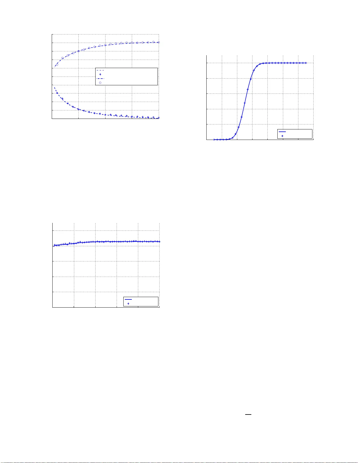
A Probability Model for Lif etime of W ireless Sensor Netw orks Moslem Noori and Masou d Ardakani Departmen t of E lectrical an d Com puter En gineerin g, Univ ersity of Alberta, CAN AD A Email: { moslem, a rdakani } @ece.ualberta. ca Abstract — Considering a wireless sensor network whose nodes are di stributed randomly ov er a gi ven area, a pr obabi lity mo del fo r the network lifetime is pro vided. Using thi s mo del and assuming that pack et generation f ollows a Poisson distribution, an analytical expression for the complementary cumulative den sity function (ccdf) of the lifetime is obtained. Usin g this ccdf, one can accurately find the probability that the networ k achiev es a giv en lifetime. It is also shown that when the number of sensors, N , is lar ge, wi th an error exponen tially decaying with N , one can predict whether or not a certain lifetime can be achiev ed . The results of this work are obtained for both multi- hop and single-hop wireless sensor networks and are v erified with computer simulation. The approaches of this paper are shown to be applicable to other packet generation models and the effect of the area shape is also inv estigated. I . I N T RO D U C T I O N W ireless s ensor networks (WSNs) are consisted of a set of cheap and usually battery-powered de v ices, called sensors. Sensor limited p ower usually necessitates a com promise b e- tween lifetime and oth er param eters such a s the d ata rate o r the q uality of th e received signal in the sink . It is usu ally impracticable to replace the sensors b atteries af ter their o pera- tion perio d. Hence, estimating the network lifetime according to the initial energy in sensors is essential fo r n etwork d esign. According to such lifetime estimatio n, o ne can cho ose the network parameters such as node density , data rate and initial energy of the sensors to achieve the desired lifetime. Lifetime a nalysis has been studied in the literatu re based on different d efinitions such as the num ber of d ead no des in the network, network coverage and network connectivity [ 1]– [6]. Authors in [ 1] derive an upper bou nd on the network lifetime co nsidering the spatial behavior of th e data source. T o achieve this go al, th ey first consider a simp lified version where the data source is a specific point, and the sou rce is connected to the sink with a straig ht line consisting of relaying sensors. Th ey d erive the op timum length o f a ho p and consequently the number of hops in the path to minim ize the total energy consumed for the data delivery . The n, they remove the assumption o f a source concentra ted on a po int and assume that the sour ce is distributed over an area. In [2] , the results o f [1] are e xten ded to the netw o rks wh ose nodes may perform d ifferent tasks of sensing, relaying and aggregating. Th e results o f [1] are also extended to m ultiple- sink n etworks in [3] . W ork reported in [4] studies the network lifetime for a cell based network. It is assum ed that N nodes are deployed over a h ypercu be. For the aim of energy con serving, th e area is divided to n hype rcubes (cells). Using o ccupancy the ory [7], the distribution of the min imum number of sen sors within each cell is inv estiga ted when N , n → ∞ . Then , a uthors study the lifetim e for the case when network rem ains almost surely connected. Using the number of sensors in each cell, the network lifetime is lower bounded based o n the gi ven lifetime of e ach sen sor . A lifetime study based on the area coverage is presented in [5 ]. It is assumed that the nodes hav e a circu lar sensing region and ar e distributed over a sq uared a rea. Using the stochastic geom etry , theory of coverage proce ss, and assuming the size o f th e area goes to infinity , an expr ession fo r the node density is derived to guarantee a k -coverage in the area. It is shown tha t using the proposed density , th e network lifetime is u pper boun ded by k T wh ere T is the giv e n lifetime of each sensor . Although the upper b ound is deri ved fo r an asymptotic situation when the area go es to in finity , it is sho wn throug h simulation th at the der iv ed bou nd is also rea sonable for networks over a finite area. Authors in [6] divide linear or circular networks to some bins where each bin c ontains a determin istically assigned number of nodes. The nodes within ea ch bin, h owe ver , are deployed rand omly . Also, the lifetime is defined as the tim e when a ho le occurs in the routing scheme (i.e. death of a bin). Assuming a fixed transmission power for e ach packet and u sing the theory of stochastic processes, au thors have found the prob ability distrib ution functio n (pdf) of the network lifetime. I n add ition, they p ropose a method to assign the number of nodes within each bin in order to maximize the network lifetime. It is worthy to n ote that other studies in the literature are perfor med on the lifetime, e.g. [8]– [12]. Ho wever , the most related ones to this work are tho se that we discussed earlier . In this paper, we find the prob ability of rea ching a cer tain lifetime f or rando mly distributed networks based on the po wer dissipation mo del o f the senso rs. Mo re spec ifically , unlike [ 4], [5], we do not assume that the lifetime of a sensor is given in order to find the network lifetime. Instead , we find the lifetime o f a sensor (as a rand om variable) based on its po wer dissipation a nd p acket g eneration m odel. Also, our analysis does not assume an infinite area and in finite number of sensors. In compar ison to [6 ], we con sider totally rando mly dep loyed networks ov er more v ariant area shapes. In addition , both fixed and adjustab le transmission po wer are studied in this work. 2 Also, the definition of lifetime in our work is more general and c an include the case studied in [6] (to be discussed in Section IV). Considering the randomne ss in pa cket generation and sensor deployment in the area, the lifetime of a ne twork is a random variable. For a lifetime analysis of the n etwork, it is need ed to have a knowledge o f the lifetime of each indi vid ual sensor . In this w or k, instead of assuming that the lifetime of each sensor is g iv en b eforeha nd, we first perf orm a life time analysis at the sensor le vel. T o th is end, we model the lifetime of a sensor as a random v ariab le and find its distribution based o n the traffic model and the power dissipation model in the sensor . Using this pro babilistic model of a sensor lifetime and the distribution of the sensors over the area, the co mplementa ry cumulative distribution fu nction (cc df) of the lif etime of a single-hop network is derived. Fr om this ccdf , the prob ability distribution fu nction (pdf ) of th e lifetime is also obtained. The single-hop analysis will be the base of our further extensions. In the pro posed analysis, no asy mptotic assump tion is made on the number of nodes. Ne verthele ss, an asymptotic analysis is provid ed, which—with an error exponen tially decaying with the num ber of senso rs—predicts whether or not a desired lifetime ca n be ach iev e d. The above analy sis is then e x tended to multi-h op network s. Since the lifetime of the multi-hop networks is depende nt on the routing scheme, we study the lifetime ccdf under th e maximum-lifetime [13] r outing. The method ologies o f this work are app licable to more general scen arios, som e of them are discussed in this paper . For exam ple, we extend the results to different traf fic models; to the case where different sensors may have different initial energy or traffic load; and to various ar ea shap es. The o rganization of this p aper is as follows. I n Section II we introd uce the system m odel a nd p rovide the required definitions and assump tions. The lifetime an alysis for single- hop networks is stud ied in Section III. Section IV discuses the lifetime analysis of multi-hop networks. Extensions to other scenarios are d iscussed in Section V and th e accuracy of the propo sed method is verified through simulations in Section VI. The p aper is co ncluded in Section VII. I I . S Y S T E M M O D E L In this section, the compon ents o f the system mod el such as li fetime definition, energy consum ption mode l and network traffic model are intr oduced . A. Lifetime Definition As mentio ned, lifetime has a g reat significance in th e design of WSNs. Con ceptually , lifetim e means the time duration that the network is operatio nal and can p erform its assigned task. Since there is no u nique m easure of the ne twork failure, the definition o f the lifetim e is app lication-rela ted. In [14]– [16] lifetime is stated as the time when the fir st node d ies. Usua lly the remain ing sensors in th e n etwork can accomplish the network’ s assigned task. Therefo re, another definition b ased on the ratio of dead n odes to the total number of nodes in the network is o ften used ( e.g. [8], [1 7], [18]). Notice tha t this definition in cludes the definitio n of lifetime based on the death of the first n ode and theref ore is more gener al. Other definitions b ased o n the comm unication connectivity o r the coverage o f the area are also pr oposed for the lifetim e [4], [5 ]. In this study , we consider the network lifetime based on the ratio o f dead no des to the total n umber of nodes, β . F or mu lti- hop networks, wh ere th e nodes clo se to the sink have mo re traffic load than other nod es and d ie soo ner, we will modify this definition. B. Energy Consumption Model The network lifetime is d irectly related to th e sensor s lifetime and in o ther words th e energy dissipated in the sensor nodes. The co nsumed energy in sensors includes the e nergy required for sen sing, recei ving , transmitting and p rocessing o f data. The total consumed e nergy is usually dom inated by the required en ergy for data tr ansmission. T wo cases may b e considered for th e tr ansmission mode of the nodes in th e network. In the first case, nodes tr ansmit with a fixed tran smission power . Th is usually results in a fixed transmission range. In the second case, nodes use a mechanism to adjust their tr ansmission power based o n th eir distance to the next ho p or the sink. Hence, the r equired energy for a packet tran smission in sensor i can b e modeled as [19 ] e ( d i ) = l ( e t d α i + e o ) = k d α i + c (1) where l rep resents the packet length in bits, d i denotes the distance between sensor i and th e next h op, α represents the path loss exponent, e t shows the lo ss coefficient related to 1 bit tr ansmission and e o is the ov erhead energy due to the sensing, receiving and processing fo r the same amou nt of data. Also, k = l e t and c = l e o represent the loss coefficient an d the overhead energy for a packet tran smission respectively . The path loss exponent dep ends o n the local terrain and is determined b y empirical measur ements. Th e typ ical value of α for WSNs is from 2 to 4 [ 18]. While this work is m ore fo cused on the transmission m odel (1), fixed transmission power is also d iscussed. C. T raffic Mo del The traf fic model of the network d epends o n the ne twork application and the behavior of sensed events. The data re port- ing pro cess in WSNs is usually classified in to th ree categories: ev en t-driven, time-driven and qu ery-d riv en [13 ]. In the time- driven case, sensors send their data periodically to the sink. Event-driven networks ar e used wh en it is desired to in form the d ata sink about the o ccurren ce of an event. In query -driven networks, sink sends a request of d ata gatherin g when need ed. In this paper, our main focus will be o n the ev en t-driven networks with Poisson model for p acket gen eration. Suppose that the e vents are indepen dent (both temporally and spatially) an d o ccur with equ al pr obability over the area. In this case, Poisson distrib u tion c an be used effecti vely to 3 model th e generation of data p ackets [6] . When the average rate o f pa cket gener ation, λ , is known, the d istribution of th e number of data packets, M , genera ted by each node, from time 0 to T is P ( M = m ) = e − λT ( λT ) m m ! (2) where m is a nonnegativ e integer number . Since the pac ket generation distribution o beys the Poisson mo del, the time duration between two consequ ent packet transmissions, t , has an expo nential distribution with mea n 1 λ : f t ( x ) = λe − xλ u ( x ) (3) where u ( x ) de notes th e unit step fu nction. W e will consid er th e Poisson model for sensor’ s traffic in this study . Howe ver, the proposed method can be exten ded to other traffic distributions and d ata gathering scena rios. I I I . L I F E T I M E A N A LY S I S I N S I N G L E - H O P N E T W O R K S In this section, we derive the pdf of the lifetime in sing le- hop WSNs. Assumin g that nod es dir ectly c ommun icate with the sink, we first deri ve the ccdf of the lifetime. Then, the pdf of the life time is obtained by taking the deri vati ve o f the ccdf. The results are extended to the case of multi-hop networks in Section IV. It is a ssumed h ere that all of the nod es have th e same initial energy , same d istribution over the area a nd the same packet generation model. Other cases like nonun iform energy distribution or different packet gener ation m odels are studied in Section V. For the ease of presentation , the list of parameter s is provided in T able I. As mentione d, the lifetime of a s in gle-hop WSN is co nsidered a s the tim e when th e ratio of dead node s to the total nu mber o f no des, N , passes a thre shold, β . N Number of deployed nodes in t he a rea β Threshold for the ratio of de ad nodes to all nodes α Path loss expon ent k Path loss coef ficient c Overhe ad energ y E i Initia l energy in sensors τ Lifeti m e threshold t i Lifetime achie ved by sensor i L Lifetime achie ved by the netw ork λ A verage rate of pa cket ge neration d i Distance of sensor i to t he ne xt hop T ABLE I P A R A M E T E R S O F T H E P R O B L E M W e start the network lifetime analysis by c onsidering the lifetime o f one sensor . Defining p i as p i = E i e ( d i ) (4) for sensor i , it is clear that the maximum n umber of p ackets that can b e tran smitted b y th is senso r is eq ual to ⌊ p i ⌋ . Lemma 1 : If a sensor node with initial energy E i is ran- domly placed in the a rea R , the probability of achieving a lifetime m ore than a thre shold τ will be P ( t i ≥ τ ) = 1 − γ ( ⌊ p i ⌋ , λτ ) Γ( ⌊ p i ⌋ ) (5) where γ ( · , · ) deno tes the lower incomplete gamma fun ction γ ( a, x ) = Z x 0 t a − 1 e − t dt (6) and Γ( · ) rep resents th e gam ma fun ction Γ( x ) = Z ∞ 0 t x − 1 e − t dt. (7) Pr oof: The lifetime of sensor i , t i , depen ds on the maximum number o f packets that can be tran smitted by the senso r to the sink. Since t i is the sum of time d uration s between packet transmissions until the last pac ket is sent by the sensor, we have t i = ⌊ p i ⌋ X j =1 t ij (8) where t ij denotes th e time duratio n between transmitting packets j − 1 and j by sensor i , and t i 1 is defined as the time when th e first packet is tran smitted. Since a Poisson model is assumed for data packet generation, t ij ’ s obey an exponential d istribution in dicated in (3). On the other hand, it is k nown that the sum of independ ent iden tically distributed (i.i.d) exponen tial random variables has a g amma distribution [20]. It is worth y to note that since the nod e is d eployed random ly in the area, the distance b etween the no de and the sink an d con sequently p i are a random variables. Hence, given p i , the conditiona l pdf of t i can b e written as follows f t i | p i ( x ) = λ ⌊ p i ⌋ x ⌊ p i ⌋− 1 e − λx Γ ( ⌊ p i ⌋ ) x ≥ 0 . (9) Now P ( t i ≥ τ | p i ) = 1 − Z τ 0 λ ⌊ p i ⌋ x ⌊ p i ⌋− 1 e − λx Γ( ⌊ p i ⌋ ) dx = 1 − γ ( ⌊ p i ⌋ , λτ ) Γ( ⌊ p i ⌋ ) . (10)  Pr oposition 1: Since the fractional part o f p i is usually much smaller th an the in teger part, ⌊ p i ⌋ ≃ p i and hence (10) can b e rewritten as P ( t i ≥ τ | p i ) = 1 − γ ( p i , λτ ) Γ( p i ) (11) For simplicity , we use (11) to analyze the network lifetime in the sequ el.  Cor ollary 1: In the case of the fixed transmission range, r , each n ode lives mor e than the threshold with p robability P ( t i ≥ τ ) = 1 − γ ( p f , λτ ) Γ( p f ) (12) 4 where p f = E i k r α + c . (13) Pr oof: I n th is case, a ll of the p i ’ s h av e a d eterministic value equal to p f . Th erefore, the value of P ( t i ≥ τ ) in ( 11) is uncon ditional and the pro of is completed by r eplacing p i by p f in (11).  One can take another ap proach an d app roximate the value of P ( t i ≥ τ ) to find a simpler form o f (1 1). Pr oposition 2: Since t i in (8) is the sum of i.i.d. random variables, central limit theorem (CL T) [20] indicates that its pdf tends to Gaussian d istribution with mean ⌊ p i ⌋ λ − 1 and variance ⌊ p i ⌋ λ − 2 . Considering ⌊ p i ⌋ ≈ p i , we h ave P ( t i ≥ τ | p i ) = Q  τ − p i λ − 1 √ p i λ − 1  . (14) where Q ( · ) is th e ccd f of the norm al distribution.  T o study the lifetime of the network , we co nsider th e lifetime of all th e nodes in the network which necessitates the k nowledge of p i for all of th e no des in the network. When a node is dep loyed ra ndomly o ver an area, p i is a random variable with pdf f p i ( x ) . In a r andom network deploym ent, p i ’ s are usually i.i.d. random v a riables and consequently ha ve the same distribution, f p ( x ) . This distribution d epends on th e shape of the area, energy dissipation model and the pdf of node distribution over the area. In the App endix, f p ( x ) is de riv e d for some com mon area shapes assuming a u niform distribution for the no de d eployment. Theor em 1: Assuming N equal-en ergy nodes are dis- tributed indep endently over the area R , the p robab ility that the n etwork achieves a lifetime more th an a given thr eshold, τ , is equal to P ( L ≥ τ ) = Q  √ N 1 − β − µ σ  (15) where µ = Z R  1 − γ ( x, λτ ) Γ( x )  f p ( x ) dx (16) σ = p µ − µ 2 . (17) Pr oof : T o find the num ber of nodes that li ve more than the lifetime thresho ld, we d efine a Bernoulli random variable l i indicating the success o f a chieving the lifetime th reshold by sensor i : l i =  1 W ith probab ility equal to s i , 0 W ith probab ility equal to 1 − s i . (18) The su ccess p robab ility of l i , giv en p i , is eq ual to s i = P ( t i ≥ τ | p i ) = 1 − γ ( p i , λτ ) Γ( p i ) (19) which was deri ved in Lem ma 1. T he nu mber of li ve no des after time τ can be found by defining a n ew ra ndom v ar iable, w , that d enotes the n umber of successes in the Bern oulli trials shown by l i ’ s w = N X i =1 l i . (20) Since nod es pac ket g eneration s are independent and p i ’ s ar e i.i.d., s i ’ s and co nsequen tly l i ’ s are also i.i.d r andom variables. In this case, w has a binom ial distribution [21 ]. Also, when the number of trials is lar g e enough, one can ap proxim ate the binomial distrib u tion with a Gaussian distrib u tion. Sinc e the number of n odes are u sually large enoug h, C L T ca n be applied on (20). Hen ce f w ( x ) = 1 √ 2 π σ w exp − ( x − µ w ) 2 2 σ 2 w (21) where µ w is the mean and σ 2 w denotes the variance of w . Fro m (20), it is clear that µ w = N X i =1 µ l i (22) where µ l i is th e mean of l i . Since l i ’ s are indepe ndent rand om variables σ 2 w = N X i =1 σ 2 l i (23) where σ 2 l i is the variance of l i . T o find the values of µ w and σ w , we need to have th e un condition al mean and variance of l i ’ s using the co nditional values. Since l i ’ s are Bernou lli random variables µ l i | p i = s i , σ 2 l i | p i = s i − s 2 i . (24) On the other hand , for two random variables x and z , the uncon ditional mean and v ar iance of x can be foun d u sing the condition al mean an d variance as f ollows [20] µ x = E [ µ x | z ] (25) σ 2 x = E [ σ 2 x | z ] + V ar [ µ x | z ] (26) where E [ · ] is th e expected value a nd V ar [ · ] deno tes the variance of the r andom variable. Using (19), (24), (25) an d (26), it can be shown that µ l i = E [ s i ] = Z R  1 − γ ( x, λτ ) Γ( x )  f p i ( x ) dx (27) σ 2 l i = E [ s i − s 2 i ] + V ar [ s i ] = E [ s i ] − E 2 [ s i ] = µ l i − µ 2 l i . (28) Since p i ’ s are i.i.d rando m v ar iables with p df f p ( x ) , we have µ l i = µ = Z R  1 − γ ( x, λτ ) Γ( x )  f p ( x ) dx ∀ i (29) σ l i = σ = p µ − µ 2 ∀ i. (30) Then, u sing ( 22) and (23) µ w = N µ, σ 2 w = N σ 2 (31) T o deri ve the probability of ach ieving the lifetime thresho ld by the network, w e just need to k now the probability of achieving the lif etime b y at least (1 − β ) N nodes. Hence F c L ( τ ) = P ( L ≥ τ ) = P ( w ≥ (1 − β ) N ) = Q  √ N 1 − β − µ σ  (32) 5 where F c L ( τ ) repr esents the ccdf of the n etwork lifetime.  Pr oposition 3: Using Pro position 2, µ can also be calc u- lated as µ = Z R Q  T thr − xλ − 1 √ xλ − 1  f p ( x ) dx. (33)  Cor ollary 2: Assuming a network with pa rameters given in Theorem 1, the probability distribution function of the network lifetime is f L ( τ ) = λ √ N 2 √ 2 π 1 − µ − β (1 − 2 µ ) ( µ − µ 2 ) 3 2 c ( τ ) e − ( λτ + N (1 − β − µ ) 2 2( µ − µ 2 ) ) 0 ≤ τ ≤ ∞ (34) where c ( τ ) = Z R f p ( x ) Γ( x ) ( λτ ) x − 1 dx. (35) Pr oof : The cc df of the n etwork lifetime was derived in the previous theorem . Then we have f L ( τ ) = − d ( F c L ( τ )) dτ = − d ( F c L ( µ )) dµ dµ dτ (36) which results in (34).  I V . L I F E T I M E A NA LY S I S I N M U LT I - H O P N E T W O R K S In mu lti-hop n etworks, the network lifetime dep ends on the way that the routin g scheme distrib u tes the traffic load among the sensor nodes. The minimum cost routing (minimum required energy or min imum number of h ops) is co n vention- ally u sed in wireless networks. Howe ver, this routing schem e cannot guaran tee the maximu m lifetime in th e n etwork [13 ]. On the o ther hand, ma ximum lifetime routing attem pts to prolon g the network lifetime by prope r traffic d istribution among the nodes. This schem e may not h av e th e minim um overall consum ed en ergy . Since we mainly focu s on the life- time analysis, we just con sider th e ma ximum life time routing. Nev e rtheless, the pro posed appr oach can be used fo r oth er routing schemes kno win g h ow the traffic is distributed among the nodes. In multi-ho p networks, the whole network traffic passes throug h the nodes in the vicinity of th e sink, hence, death of th ese nod es can have a significant effect on the network perfor mance. Therefo re, we n eed to m odify our previous definition o f the lifetim e. Assume that H shows the set of nodes that are in the vicinity of the sink and d irectly commu nicate with it. Since all o ther nodes communica te to the sink thr ough t hese nodes, they will be out of energy soo ner than th e other on es. So, we d efine the lifetime based on the ratio of dead nodes within H to |H| where | · | denotes the cardinality of the set. It is also assumed that th e sensors are d istributed over a cir cle with radius R and the data sin k is positioned at the center of the area. The lifetime of th e ne twork over other area shapes will be discussed later . W e assum e that the sensors per form transmission with a fixed power wh ich re sults in a fixed transmission rang e r . Based on the maximum transmission radius of the sensors and the area r adius, the area can b e divided to a n umber of rings (Figure 1). The sensor s with in a ring send their data to the sensors within th e neighb oring inner rin g. The n umber of rings, n , within the area can be simp ly fo und as n =  R r  (37) where ⌈·⌉ den otes the integer ce iling. For simp licity , it is assumed that R is an integer multiple of r . This assum ption allows u s to focus o n metho dolog ies and can be removed if necessary . I n addition, since each ring carries the tr affic of all outer rings, th e a verage traffic carried by the sensors with in each ring is different and depen ds on the distance of the ring to the sink . T o study the network lifetim e, we con sider the case when the routing scheme distrib u tes the network traf fic equally between the nodes within each ring. Th is scheme prev e nts the nodes fr om bein g exhau sted quickly a nd pro longs the lifetime . R r r r Fig. 1. Rings within a multi-hop network Based on th e assumed routing scheme, the average rate of the packet tran smission by each node within rin g i is equ al to λ i = λ N − P i − 1 j =1 N j N i ∀ i = 1 , 2 , . . . , n (38) where N i denotes the nu mber o f sensors within r ing i . Since nodes are assum ed to b e deployed ran domly in the area, N i is a binomial rand om variable. If one assumes a uniform deployment for the nodes, N i will have a bino mial distribution with me an N q i where q i = r 2 (2 i − 1) R 2 (39) represents th e probability o f p ositioning a sensor in the ring i . Therefo re, the time du ration betwee n two conseq uent trans- missions, t , by a nod e in the rin g i o beys an exponential distribution as follows f t | N i ( x ) = λ i e − xλ i u ( x ) . (40) Since the lif etime is mainly effected by the no des within the first tier, we just co nsider the probability o f achieving the lif e- time th reshold b y the first ring . Nevertheless, the pro bability of achieving τ by other rings can also b e inv e stigated using (40). As d iscussed earlier, pro bability of achieving a lifetime 6 threshold depends on the number of nodes with in the area. Hence, using Theore m 1 and Corollary 1, on e can find the condition al prob ability of ac hieving τ by th e first r ing P ( L ≥ τ | N 1 ) = Q  p N 1 1 − β − µ σ  (41) where µ = 1 − γ ( p f , λ 1 τ ) Γ( p f ) (42) σ = p µ − µ 2 . (43) Therefo re, b y removing th e cond ition o n N 1 in (41), we ha ve P ( L ≥ τ ) = N X j =0 P ( L ≥ τ | N 1 ) P ( N 1 = j ) n 1 = 1 , 2 , . . . , N (44) where P ( N 1 = n 1 ) =  N n 1  q n 1 1 (1 − q 1 ) N − n 1 . (45) The given discussion is not r estricted to circu lar areas and can also be applied to other area s h apes. T o study the lifetime of the n etwork in other area shapes, we ju st need to r ecalculate the value of q 1 as f ollows q 1 = π r 2 S (46) where S is the size of area. Then, ccdf of the lifetime is deri ved by putting this value of q 1 into ( 44). V . S O M E N O T E S In Section III, we con sidered the finite n umber of nod es in the area. W e will study th e asymp totic an alysis in this section . Also, we earlier studied th e case when all o f the sen sors have the same featur es su ch as traffic mod el, initial energy and dep loyment. In ad dition, the packet gen eration mod el was supposed to b e Poisson. Here, we provide some discussions on the re sults in Section III and gene ralize them f or m ore cases. A. Asymptotic Analysis Since th e lifetime ccdf in (15) de pends o n th e nu mber o f nodes distributed o ver the area, we can study the effect of the nod e d ensity on the pr obability of achieving the life time threshold. Cor ollary 3: The p robab ility of ach ieving a lifetime thresh- old a pproach es 0 o r 1 b y inc reasing the nu mber o f no des. Pr oof: For large N , tw o cases can h appen depending on the sign of a = 1 − β − µ . Since Q - function is a dec reasing function , when a > 0 , increasing N causes the prob ability of hitting th e lifetime threshold to tend Q ( ∞ ) = 0 . I n othe r words, almo st surely the given lif etime threshold canno t be achieved. No w , considering that [2 2] 1 √ 2 π x  1 − 1 x 2  e − x 2 2 < Q ( x ) < 1 √ 2 π x e − x 2 2 ∀ x ≥ 0 (47) the rate of the pro bability decay is propor tional to e − N . In a similar man ner, the proba bility approach es Q ( −∞ ) = 1 when a < 0 . That is, the network almo st surely achieves the lifetime th reshold. T he error in this prediction also de cays exponentially with N .  An interesting case occu rs when on e considers the lifetime of the network based on the death of th e first nod e. I n this case β = 1 N , wh ich app roaches 0 wh en N increases. Hen ce, accordin g to the Corollary 3, it is necessary to consider just the sign of 1 − µ in order to pr edict th e asympto tic beh avior of the n etwork life time (i. e. when N → ∞ ) . Assumin g τ > 0 , we hav e µ = Z R  1 − γ ( x, λτ ) Γ( x )  f p ( x ) dx < Z R f p ( x ) dx = 1 (48) and co nsequently 1 − µ > 0 . Therefore, under th is stringen t definition o f th e lifetim e, th e probability of achieving the lifetime τ ap proach es 0 as N increases. B. Differ ent T raffic Models In Sec tion III, we c onsidered the case when all of the sen- sors h av e the same Poisson mod el for the packet gen eration. Here, we consider two other cases: 1) The average rate of packet generation chang es with the position o f the sensor, 2) packet generation obeys an other model rather than P oisson. It is worth y to note that the assumed mo del is similar fo r all of the senso rs. If the average rate of packet generatio n, λ , varies w ith the position of th e sensor ( e.g. du e to the spatial correlation of data or data ag gregation an d compression), we have th e mean and variance of l i condition ed on both p and λ . T o derive the uncon ditional mean an d variance o f l i , we n eed to calculate µ l i = µ = Z Z R  1 − γ ( x, λy ) Γ( x )  f p,λ ( x, y ) dxdy (49) where f p,λ ( x, y ) de notes the joint pdf o f p and λ . Oth er parts of th e analysis will remain unch anged. Also, the proof given for Theorem 1 can be applied to the cases when the traffic model o beys another pattern rathe r than Poisson model. Assume that the pdf of the time duration be- tween two packet transmissions fo llows a m odel with mean µ t and v arian ce σ 2 t . Using CL T , t i can be accurately approxima ted by a Gaussian distribution with mean p i µ t and v a riance p i σ 2 t . The r emaining part o f the pr oof is unch anged. The p ropo sed analysis can also b e extend ed to time-dr iv en networks. I n this case, the time du ration between two conse- quent tra nsmissions is fixed and is equ al to T . Hen ce t i = ⌊ p i ⌋ T . (50) The uncon ditional values o f µ and σ is f ound by in tegration over p i . Then, the resu lt g iv en in Th eorem 1 can be applied. C. Non uniform Ener g y Distribution Assume th at the energy is distributed over the network in a no nunifo rm way . As a consequ ence, s i ’ s in ( 19) are not identically distributed. This may also arise when the sensors generate p ackets with d ifferent rates (i.e. no nidentical Po isson distributions). In this situa tion, w do es not have any standar d 7 distribution, however , we can still use CL T to approxima te the pdf of w with a Gaussian distribution. T o this end, we will giv e a br ief discussion o n the probability of achieving the lifetime threshold by the ne twork. Lemma 2 : Assume th at z i ’ s ( 1 ≤ i ≤ m ) are m ind epen- dent random variables such th at m X i =1 µ z i = m µ. (51) where µ z i denotes the mean of z i . Also, X i ’ s ( 1 ≤ i ≤ m ) are m Berno ulli trials such that P ( X i = 1) = z i ∀ i. (52) Now , if X denotes the sum of X i ’ s, the variance of X is maximum when µ z i = µ ∀ i = 1 , . . . , m (53) (see [21] fo r th e pr oof). Cor ollary 4: For n onidentica l distrib u ted s i ’ s such th at µ w = N X i =1 µ l i = N X i =1 E [ s i ] = N µ (54) (15) is an u pper bo und for the pr obability of achie vin g the lifetime wh en 1 − β − µ > 0 , other wise it is a lower b ound. Pr oof: Since we a ssumed the identical distribution in the proof o f Th eorem 1, Lemma 2 indicates that σ w in (3 1) is the maximum possible variance of w . T he proof is completed considerin g the decreasing p roperty of th e Q -f unction.  V I . E X P E R I M E N TA L R E S U LT S In this section, we in vestigate the ac curacy of the pro- posed an alysis thr ough some exper iments. W e first stud y th e probab ility of a chieving a lifetime thr eshold in single-hop networks. T o th is en d, the simulatio ns are perfor med over different area shapes with th e same ar ea size to in vestigate the effect of the area shape. In addition , the e ffect of the node d ensity is studied . Mor eover , simulations ar e per formed to study the network lifetime in multi-hop networks. T hroug h these simulations, it will be shown that how the transmission range an d c onsequen tly the number of hops effect the lifetime of th e network. A. Single- hop Networks The parame ters of model (1) d epend on the data rate, antenna heigh t, antenna gain, etc. T ypical values of e t and e o are given in [23]. For α = 4 , which we use in our simulation s, the values of e t and e o are r espectiv ely 0.00 13 pJ/bit/m 4 and 50 nJ/bit for a 1 Mbps data strea m. Here, It is assumed that the packets ha ve 100 0 b its leng th, henc e, k = 1.3 pJ/m 4 and c = 50 µ J in ( 1). Network has 500 nodes th at are deployed uniformly and sink is positioned at the ce nter of the area. Also, the pac ket generation model obeys the Poisson distribution an d each sensor s e nds its packets d irectly to the sink. All o f the sensors have th e same initial energy equ al to 11 mJ. Assuming tha t sensors sen d p acket with th e average rate of 1 p acket/hour, the probab ility o f ac hieving the lifetime of 100 hours is studied throug h simulation. T o invest igate the effect of th e area shape on the lifetime, the simulation s a re carried o ut over ar eas with the same size equal to 100 π m 2 but with dif f erent shapes. T o d ecrease the final resu lt variance a nd reach the proper confidence in terval, the simulation is run 10000 times o ver each ar ea and the results are averaged. Figure 2 depicts the p robab ility of ach ieving the lifetime threshold vs. the ratio of dead n odes over circular, hexago nal, squared a nd triang ular are as. As it can be s e en, the p robab ility of achieving the lifetime thresho ld in circular, hexagonal and squared a reas are very c lose. Since in a triang le, the distance of th e sensors to the sink is more n on-u niform and it h as the largest circumc ircle compar ed to other area shapes, triang le has a smaller pro bability to achieve the life time thr eshold. 0.2 0.25 0.3 0.35 0.4 0.45 0 0.2 0.4 0.6 0.8 1 Ratio of dead nodes ( β ) P(L>100) Circle (Analytical) Circle (Simulation) Hexagon (Analytical) Hexagon (Simulation) Square (Analytical) Square (Simulation) Triangle (Analytical) Triangle (Simulation) Fig. 2. Probabilit y of achie ving the l ifetime threshol d vs. the ratio of dead nodes for single-hop networks deploye d ove r dif ferent are a shapes As d iscussed thr ough the paper, depending o n the value of 1 − µ − β and by increasin g the n umber of nod es, it can be a lmost surely deter mined wheth er th e n etwork achieves a lifetime thresho ld or not. The effect of the nod e density on achieving the lifetime thresho ld is shown in Figur e 3. The lifetime o f th e network is considere d as the moment when 0.3 of the no des in the n etwork die. In th e first case, E i = 11 mJ which resu lts in 1 − β − µ > 0 . Hence, as d iscussed in Section V, the desired pro bability dec reases by increasing N which is verified by the simulation. In the second case, the initial en ergy is equal to 11.6 mJ which causes 1 − β − µ < 0 . As shown in Figure 3, the proba bility of achie v ing the desired lifetime is a n incr easing fu nction of N . B. Multi-hop Networks T o study the network lifetime in a multi-hop network , it is assumed that 50 0 no des are deployed u niformly over a circle with rad ius 100 m. All of the n odes have the same initial energy equal to E i = 100 mJ. The par ameters in (1) are kept the same as the previous part. A greedy rou ting algo rithm is u sed to balance the network traffic su ch th at da ta pac kets 8 0 500 1000 1500 2000 0 0.1 0.2 0.3 0.4 0.5 0.6 0.7 0.8 0.9 1 Number of sensors (N) P(L>100) Decreasing Probability (Analytical) Decreasing Probability (Simulation) Increasing Probability (Analytical) Increasing Probability (Simulation) Fig. 3. Probabil ity of achie ving the lifetime threshold vs. the number of sensors in a single-hop network are id entically d istributed between the node s in the first ring of th e ne twork, H . Considering this fact that all of the n odes use a constant tran smission power and th e traffic is distributed identically b etween the fir st-ring no des, all of the nodes within H ha ve approximately similar lifetime. As a consequence, the y die in time mo ments very close to ea ch othe r . T herefor e, we can say that the desired prob ability is no t significantly effected by the v alue of β (Figure 4). 0 0.1 0.2 0.3 0.4 0.5 0 0.2 0.4 0.6 0.8 1 Ratio of dead nodes ( β ) P(L>100) Analytical result Simulation result Fig. 4. Probabilit y of achie ving the l ifetime threshol d vs. the ratio of dead nodes in a multi-hop network It is interesting to study the ef fect of the tr ansmission ran ge and consequ ently the number of h ops on the lifetim e. Figure 5 de picts the prob ability of r eaching th e lifetime thresh old vs. th e transmission range. T he lif etime is considered as the moment wh en 0.3 n odes within H are dead. By de creasing r , n umber o f no des within H decr eases, hence, th ey carry more packets and will die earlier . Therefor e, it is expected that the desired p robab ility de creases by r educing r . In deed, while the nodes f a r from the sink still hav e enough en ergy to send packets, the nodes within H cease. T o overcome this drawback, nonun iform energy distribution can be app lied [24 ]. Also, the fixed transmission power cau ses the nod es within H to die sooner co mpared to the case wher e n odes adjust their transmission power . 10 15 20 25 30 35 40 45 0 0.2 0.4 0.6 0.8 1 Transmission range R t P(L>100) Analytical result Simulation result Fig. 5. Probabil ity of achie ving the lifet ime threshol d vs. th e tra nsm ission range in a multi-hop network V I I . C O N C L U S I O N S In this pa per, we co nsidered the pro blem o f finding the probab ility of achieving a lifetime thresho ld b y th e network which is equ iv alent to find ing the ccdf of the network lifetime. Using the power consu mption mod el of (1), th e ccdf of the lifetime was deri ved fo r the single-hop networks. T o this end, it was assum ed that all of the nodes h av e identical p acket generation model, initial energy and ra ndom d eployment in the area. The method ology was also extended to the case when these co nditions ma y not be satisfied. Then, th e pr oblem was studied for the multi-hop case. In add ition, th e asymp totic relation between the number of nodes an d the lifetime was in vestigated. Thro ugh some simulations, the accuracy of our analysis was inves tigated fo r the n etworks dep loyed over different a rea shap es. Using the p roposed method , one can design both node an d network par ameters (e.g. no de den sity , data r ate, initial energy ) according to the desired lifetime. A P P E N D I X The pdf o f the network lifetime depends on the distribution of the maximu m po ssible number of packet transmissions by each nod e, p . In th is ap pendix , we find the p df of p over some comm on area shape s. The pdf of p over a circle a rea is required for findin g the lifetime pd f of multi-ho p networks in Section IV. Also, this pdf over regular p olygon s is useful for studying the lif etime of a n etwork c omposed of clusters tilin g the ar ea. A. Network Deployed Over a Cir cle Assume th at the nodes are deployed unifor mly over a circle with radius R . Also, assume that th e sin k is located at the center of the circle. Since the nod es are dep loyed u niform ly over the area, th e pdf of th e distance b etween the node s and sink, d , is f d ( x ) =  2 x R 2 0 < x ≤ R 0 Otherwise . (55) 9 Now , using the energy con sumption mo del ( 1), we have the following expression fo r the pdf of p f p ( x ) = ( 2 E i R 2 kαx 2  E i − cx kx  2 − α α E i kR α + c ≤ x < E i c 0 Otherwise . (56) B. Network Deployed Over a Regular P olygo n Suppose th at the sensors are deployed over a regular poly- gon having n equal sides with len gth a . Again, we assume that th e sink is p laced at the center of the area. In th is case, we hav e f d ( x ) =    2 π x S 0 < x ≤ r i 2 π x − 2 nx cos − 1 r x S r i < x ≤ R c 0 Otherwise (57) where r i = a 2 cot π n (58) is th e radius o f the inscr ibed circle of the polygon , R c = a 2 sin π n (59) represents the rad ius o f the circu mcircle of the poly gon and S = n 4 a 2 cot π n (60) denotes the poly gon are a. Now , using the relatio n between d and p , we have f p ( x ) = 2 E i k αS x 2  E i − cx k x  2 − α α   π − n cos − 1 r  E i − cx kx  1 α   (61) when E i k R α c + c ≤ x < E i k r α i + c and f p ( x ) = 2 π E i k αS x 2  E i − cx k x  2 − α α (62) when E i k r α i + c ≤ x < E i c and f p ( x ) = 0 elsewhere. R E F E R E N C E S [1] M. Bhardwaj , T . Garnett, and A. P . C handrakasan, “Upper bounds on the lifetime of sensor netwo rks, ” in Communications, 2001. ICC 2001. IEEE International C onferenc e on , v ol. 3, Helsinki, Finland, 20 01, pp. 785–790. [2] M. B hardwaj and A. P . Chandraka san, “Bo unding the lifeti m e of sensor netw orks via optimal role assignments, ” in INFOCOM 2002. T wenty- F irst Annual Joi nt Co nferenc e of t he IEEE Computer and Communi ca- tions Societie s . Pr oceedings. IEEE , vol. 3, 2002, pp. 158 7–1596. [3] A. P . Azad and A. Chockalin gam, “WLC12-2: Bo unds on the lifet ime of wireless sensor net works employin g multiple data sinks, ” i n Global T e lecommuni cations Conf er ence, 2006. GLOBECOM ’06. IEEE , San Francisco , CA, USA, Nov . 2006, p p. 1–5. [4] D. M. Blough and P . Santi, “In vestigati ng uppe r boun ds on netw ork lifeti m e extensio n for cell-b ased energ y conserv ation techniques in station ary ad hoc netwo rks, ” in Mobi Com ’02: Pr oceedin gs of the 8th annual international conf erence o n Mobile comput ing and ne tworking . Ne w Y ork, NY , USA: AC M Press, 2002, pp. 183– 192. [5] H. Zhang and J. Hou, “On de riving t he upper bound of α -lifetime for larg e sensor netwo rks, ” in Mobi H oc ’04: P r oceedings of the 5th ACM internat ional symposium on Mobile ad ho c networking and computing . Ne w Y ork, NY , USA: AC M Press, 2004, pp. 121– 132. [6] V . Rai and R. N. Mah apatra , “Lifetime modeling of a sensor netwo rk, ” in DATE ’05: Proc eedings of the confer ence on Design, Automation and T e st in Eur ope . W ashington, DC, USA: IEEE Compu ter Society , 2 005, pp. 202–203. [7] V . Kolci hn, B. Se vast’ya nov , and V . Chistyako v , Random A llocat ions , A. V . Balakrishn an, Ed. W ashingt on D.c.: W inston a nd Sons, 1978. [8] E. J. Duarte-Melo and M. Liu, “ Analy sis of ener gy consumption and lifeti m e of heterogene ous wireless sensor netwo rks, ” i n Global T elecom- municati ons Confe rence , 2002. GLOBECOM ’02. IEEE , vol. 1, Nov . 2002, pp. 21–25. [9] Q. Xue and A. Ganz, “On the lifetime of la rge scale sensor ne tworks, ” Elsevi er Journal on C omputer Communicati ons , vol. 29, pp. 502–510, 2006. [10] S. Baydere , Y . Safkan, and O. D. Incel, “Lifetime analysis of reliable wireless sensor ne tworks, ” IEICE T ransacti ons on Communi cations , pp. 2465–2472, 2005. [11] Y . Chen and Q . Zhao, “On the lifetime of wireless sensor networks, ” IEEE Communic ations Let ters , vol. 9, no. 11, pp. 976–978, No v . 2005. [12] S. Coleri, M. Ergen, and T . J . Koo, “Life time analysis of a sensor netw ork with hybrid automata modelling, ” in WSN A ’02: Pro ceedings of the 1st ACM internation al workshop on W ire less sensor networks and applica tions . Ne w Y ork, NY , USA: AC M Press, 2002, pp. 98–1 04. [13] J. N. Al-Karaki and A. E. Kamal, “Routing techni ques in wireless sensor netw orks: a s urve y , ” IEEE [see also IEEE P ersonal Communicat ions] W ir eless Communi cations , vol . 11, no. 6, pp. 6–28, Dec. 2 004. [14] W . B. Heinzelman, A. P . Chandraka s an, and H. Balakri s hnan, “ An applic ation-specific protocol architect ure for wireless microsensor net- works, ” IEEE T ransactio ns on W ir eless Communi cations , vol . 1, no. 4, pp. 660–670, Oct. 2002. [15] R. Madan and S. Lall, “Distrib uted algorithms for maximum lifet ime routing in wireless sensor networks, ” IEEE T ransaction s on W ir eless Communicat ions , vol. 5, no. 8, pp. 2185–2193, Aug. 2006 . [16] J.-H. Chang and L. T assiulas, “Energ y conserving routing in wireless ad- hoc networks, ” in INFOCOM 2000. Nineteenth Annual J oint Confere nce of the IEEE Computer and Commun ications Societ ies. Pro ceedings. IEEE , vol. 1, T el A vi v , Israe l, Mar . 2000, pp. 22–31. [17] Y . Xu, J. Heidemann, and D. Estrin, “Geography-in formed energy conserv ation for ad hoc rout ing, ” in MobiCom ’01: P r oceedings of the 7th annual internati onal confer ence on Mobile computing and networki ng . New Y ork, NY , USA: ACM Press, 2001, pp. 70–84. [18] E. I. Oyman and C. Ersoy , “Multiple sink network design problem in larg e scale wirel ess sensor netw orks, ” in Communication s , 2004 IEEE Internati onal Confer ence on , vol . 6, June 2004, pp. 3663–3667. [19] W . R. Heinzelman, A. Chandrakasan, and H. Balakrish nan, “Energy- ef ficient communic ation protoc ol for wireless microsensor networks, ” in HICSS ’00: Pr oceedings of the 33rd Hawa ii Internat ional Confer ence on System Scie nces , vol. 8. W ashi ngton, DC, USA: IEEE Comput er Society , Jan. 2000, pp. 30–37. [20] S. M. Ross, Intr oduction to Pr obability Models , 7th ed. San Diego , US: Academic Press, 2000. [21] J. Nedel m an and T . W all enius, “Bernoulli trials, Poisson trials, surprisi ng v ariances, and Jensen’ s inequali ty , ” Journal of American Statistici an Association , vol. 40, no. 4, pp. 286–289, Nov . 1986. [22] J. G. Proakis and M. Salehi, Communi cation Systems Engineering , 2nd ed. Upper Saddle Ri ver , NJ, USA: Prent ice-Hall, 2004. [23] W . B. Heinzel m an, “ Applicat ion-specific prot ocol for wireless net- works, ” Ph.D. dissertation, Massachusetts Institute o f T echnology , 2000. [24] S. Phoha, T . F . L. Porta, and C . Grif fin, Eds., IEEE M onogr aph on Sensor Network Operati ons , 6th ed. San Diego, US: IEEE Press, 2004.