Bayesian Classification and Regression with High Dimensional Features

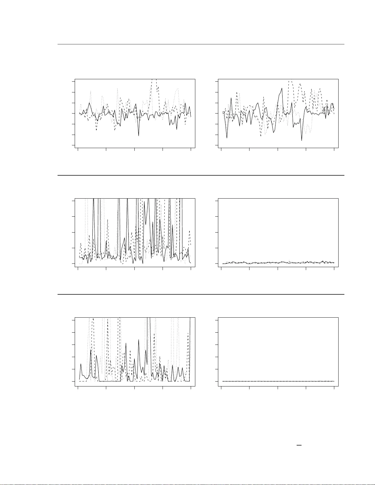
BA YESIAN CLASSIFICA TION AND REGRESSION WITH HIGH DIMENS IONAL FEA TURES Longhai Li A thesis submitted in confor mity with the requirem en ts for the degree of Do ctor of Phil osophy Graduat e D epart m en t of S t atist ics Universit y of T oronto c  Cop yrigh t 2007 Longhai Li Ba y esian Classiﬁcation and Regre s sion with High Dimensional F eatures Longhai Li Submitt ed for the Degree of Doct or of Philoso ph y August 2007 Abstract This thesis respo nds to the c hallenges of using a large n um b er, suc h as thousands, of features in regression and classiﬁcation problems. There are tw o situations where suc h high dimensional features arise. One is when high dimensional measuremen ts are av ailable, for example, gene expression data pro duced b y microarra y tec hniques. F or computationa l or other reasons, p eople may select only a small subset of features when mo delling suc h data, b y lo oking a t ho w relev an t the features a re t o predicting the resp onse, based on some measure suc h as correlation with the resp onse in the training data. Although it is used v ery commonly , this pro cedure will mak e the resp onse app ear more predictable than it actually is. In Chapter 2, w e prop ose a Ba y esian metho d to a v o id this selection bias, with a pplication to naive Bay es mo dels and mixture mo dels. High dimensional features a lso arise when w e consider high-order in teractions. The n um- b er of para meters will increase expo nen tia lly with the order considered. In Chapter 3, w e prop ose a metho d for compressing a group of parameters in to a single one, by exploiting the fact that many predictor v ariables deriv ed fro m high- order in teractions hav e the same v alues for all the training cases. The num b er of compressed parameters may hav e conv erged b efore considering the highest p ossible order. W e apply this compression metho d to lo g istic sequence prediction mo dels and logistic classiﬁcation mo dels. W e use b oth sim ulated dat a and real data to test o ur metho ds in b oth ch apters. ii Ac k no wledgem e n ts I can neve r ov erstate m y gratitude to my supervisor Professor Radford Neal who guided me throughout the whole PhD training p erio d. Without his inspiration, conﬁdence, and insigh t f ul criticism, I w ould hav e lost in the course of pursuing this degree. It has b een m y so fa r most v aluable academic exp erience to learn from him how to p onder problems, how to in v estigate them, how to w ork on them, and how to presen t the results. I w ould lik e to thank m y PhD advisory and exam committee mem b ers — Professors La wrence Brunner, Radu Craiu, Mik e Ev ans, Keith Knigh t, Jeﬀrey Rosen thal and F ang Y ao. Their commen ts enhance this ﬁnal presen tation. Most of t he aforemen tioned professors, and in addition Professors Andrey F euerv erger, Nancy Reid, Muni Sriv astav a, and Lei Sun, hav e taugh t me in v arious g raduate courses. Muc h know ledge f rom them has b ecome part of t his thesis silen tly . I wish to specially tha nk m y external appraiser, Professor Andrew Gelman. Many of his commen ts ha v e greatly improv ed the previous draft of this thesis. I am grateful t o the supp o rt pro vided b y the statistics departmen t staﬀ — Laura Kerr, Andrea Carter, Dermot Wheland and Ram Mohabir. The y hav e made the studen t life in this departmen t so smo ot h and enjo y able. I am indebted to m y many studen t colleagues, who a ccompanied and shared kno wledge with me. Sp ecial thanks go to Shelley Cao , Meng D u, Ana-Maria Staicu, Sh uying Sun, T ao W ang, Jianguo Zhang, Sophia Lee, Babak Shah bab, Jennifer Listgart en, and man y others. I would like to thank my wife, Y eh ua Zhang. It w ould hav e b een imp ossible to ﬁnish this thesis without her supp ort and lo v e. I wish to thank my sister, Meiw en Li. She pro vided me with m uc h supp ort at the most diﬃcult time to me. The la st and most imp ort a n t thanks go to my paren ts, Bao qun Jie and Y ansheng Li. They b ore me, raised me and suppo rted me. T o them I dedicate this thesis. iii Con ten ts 1 In tro duction 1 1.1 Classiﬁcation and Regression . . . . . . . . . . . . . . . . . . . . . . . . . . . 1 1.2 Challenges of Using High Dimensional F eatures . . . . . . . . . . . . . . . . 4 1.3 Tw o Problems Addressed in this Thesis . . . . . . . . . . . . . . . . . . . . . 6 1.4 Commen ts on the Bay esian Approach . . . . . . . . . . . . . . . . . . . . . . 7 1.5 Mark ov Chain Mon te Carlo Metho ds . . . . . . . . . . . . . . . . . . . . . . 10 1.6 Outline of the Remainder o f the Thesis . . . . . . . . . . . . . . . . . . . . . 12 2 Av oiding Bias from F eature Selection 13 2.1 In tro duction . . . . . . . . . . . . . . . . . . . . . . . . . . . . . . . . . . . . 14 2.2 Our Metho d for Av oiding Selection Bias . . . . . . . . . . . . . . . . . . . . 16 2.3 Application to Ba y esian Naive Bay es Mo dels . . . . . . . . . . . . . . . . . . 23 2.3.1 Deﬁnition of the Binary Naive Ba y es Mo dels . . . . . . . . . . . . . . 23 2.3.2 In tegrating Aw a y ψ and φ . . . . . . . . . . . . . . . . . . . . . . . . 25 2.3.3 Predictions for T est Cases using Numerical Quadrature . . . . . . . . 27 2.3.4 Computation of the Adjustmen t F a ctor for Naiv e Ba y es Mo dels . . . 29 2.3.5 A Simulation Exp erimen t . . . . . . . . . . . . . . . . . . . . . . . . 33 2.3.6 A T est Using Gene Expression Da ta . . . . . . . . . . . . . . . . . . . 40 2.4 Application to Ba y esian Mixture Mo dels . . . . . . . . . . . . . . . . . . . . 44 2.4.1 Deﬁnition of the Binary Mixture Mo dels . . . . . . . . . . . . . . . . 44 iv 2.4.2 Predictions for T est Cases using MCMC . . . . . . . . . . . . . . . . 47 2.4.3 Computation of the Adjustmen t F a ctor for Mixture Mo dels . . . . . . 51 2.4.4 A Simulation Exp erimen t . . . . . . . . . . . . . . . . . . . . . . . . 52 2.5 Conclusion and Discussion . . . . . . . . . . . . . . . . . . . . . . . . . . . . 57 App endix 1: Pro of of the we ll-calibration of the Ba y esian Prediction . . . . . . . . 58 App endix 2: Details of the Computation of the Adjustmen t F actor for Binary Mixture Mo dels . . . . . . . . . . . . . . . . . . . . . . . . . . . . . . . . . . 60 3 Compressing P arameters in Ba y esian Mo dels with High-order Interactions 63 3.1 In tro duction . . . . . . . . . . . . . . . . . . . . . . . . . . . . . . . . . . . . 64 3.2 Tw o Mo dels with High-o r der Inte ractions . . . . . . . . . . . . . . . . . . . . 66 3.2.1 Ba y esian Logistic Sequence Prediction Mo dels . . . . . . . . . . . . . 66 3.2.2 Remarks on the Sequence Prediction Mo dels . . . . . . . . . . . . . . 69 3.2.3 Ba y esian Logistic Classiﬁcation Mo dels . . . . . . . . . . . . . . . . . 70 3.3 Our Metho d for Compressing Parameters . . . . . . . . . . . . . . . . . . . . 73 3.3.1 Compressing P arameters . . . . . . . . . . . . . . . . . . . . . . . . . 73 3.3.2 Splitting Compressed Parameters . . . . . . . . . . . . . . . . . . . . 75 3.3.3 Correctness of the Compressing-Splitting Pro cedure . . . . . . . . . . 76 3.3.4 Sampling from the Splitting D istribution . . . . . . . . . . . . . . . . 78 3.4 Application to Sequence Prediction Mo dels . . . . . . . . . . . . . . . . . . . 82 3.4.1 Grouping P arameters of Sequence Prediction Mo dels . . . . . . . . . 82 3.4.2 Making Prediction for a T est Case . . . . . . . . . . . . . . . . . . . 86 3.4.3 Exp eriments with a Hidden Marko v Mo del . . . . . . . . . . . . . . . 87 3.4.4 Sp eciﬁcations of the Priors and Computation Metho ds . . . . . . . . 88 3.4.5 Exp eriments with English T ext . . . . . . . . . . . . . . . . . . . . . 95 3.5 Application to Logistic Classiﬁcation Mo dels . . . . . . . . . . . . . . . . . . 102 3.5.1 Grouping P arameters of Classiﬁcation Mo dels . . . . . . . . . . . . . 102 v 3.5.2 Exp eriments Demonstrating Parameter Reduction . . . . . . . . . . . 107 3.5.3 Exp eriments with Data fro m Cauc h y Mo dels . . . . . . . . . . . . . . 109 3.6 Conclusion and Discussion . . . . . . . . . . . . . . . . . . . . . . . . . . . . 109 Bibliograph y . . . . . . . . . . . . . . . . . . . . . . . . . . . . . . . . . . . . . . 115 vi List of Figures 2.1 A dir ected graphical mo del f o r the general class of mo dels . . . . . . . . . . 20 2.2 A picture of Ba y esian naiv e Bay es mo dels. . . . . . . . . . . . . . . . . . . . 24 2.3 Displa y of sample correlations with an example . . . . . . . . . . . . . . . . 31 2.4 Scatter plot of sample correlations in the training set and the t est set . . . . 34 2.5 Comparison of actual and exp ected error rates using sim ulated data . . . . . 36 2.6 P erfo rmance in t erms of av erage min us lo g pr o babilit y and av erage squared error using sim ulat ed da ta . . . . . . . . . . . . . . . . . . . . . . . . . . . . 36 2.7 P o sterior distributions of log ( α ) fo r the sim ulated data . . . . . . . . . . . . 39 2.8 Scatterplots o f the predictiv e probabilities of class 1 for the 10 subsets dra wn from the colon cancer gene expression data . . . . . . . . . . . . . . . . . . . 42 2.9 Actual v ersus exp ected error rates on t he colon cancer datasets . . . . . . . . 43 2.10 Scatterplots of the av erage minus log probabilit y o f the correct class a nd of the a v erage squared error . . . . . . . . . . . . . . . . . . . . . . . . . . . . . 43 2.11 A picture o f Bay esian binar y mixture mo dels . . . . . . . . . . . . . . . . . . 45 2.12 Notat io ns used in deriving the adjustmen t factor of Ba y esian mixture mo dels 51 2.13 Actual a nd exp ected error rates with v arying num b ers of features selected . . 54 2.14 Pe rformance in terms o f av erage min us log probability and av erage squared error b y sim ulated data . . . . . . . . . . . . . . . . . . . . . . . . . . . . . . 54 vii 3.1 A picture of the co eﬃcien ts, β , for all patterns in binary sequence s of length O = 3. . . . . . . . . . . . . . . . . . . . . . . . . . . . . . . . . . . . . . . . 67 3.2 A picture displa ying all the in teractio n patterns of classiﬁcation mo dels . . . 71 3.3 A picture depicting the sampling pro cedure after compressing parameters. . 75 3.4 A picture showing tha t the interaction patterns in log istic sequence prediction mo dels can b e g roup ed, illustrated with binary sequences of length O = 3, based on 3 training cases . . . . . . . . . . . . . . . . . . . . . . . . . . . . . 84 3.5 The algorithm f o r grouping para meters of Ba y esian lo g istic sequence predic- tion mo dels. . . . . . . . . . . . . . . . . . . . . . . . . . . . . . . . . . . . . 85 3.6 A picture sho wing a Hidden Mark ov Model, whic h is used to generate se- quences to demonstrate Bay esian log istic sequenc e prediction mo dels . . . . 88 3.7 Plots sho wing the reductions of the num b er of parameters and the training time with our compression metho d using the exp eriments on a data set g en- erated b y a HMM . . . . . . . . . . . . . . . . . . . . . . . . . . . . . . . . . 92 3.8 The auto correlation plots of the Mark o v c hains of σ o ’s for the experimen ts on a data set generated by a HMM . . . . . . . . . . . . . . . . . . . . . . . . . 93 3.9 Plots show ing the predictiv e p erfor ma nce using the exp erimen ts on a data set generated b y a HMM . . . . . . . . . . . . . . . . . . . . . . . . . . . . . . . 94 3.10 Plots showing the reductions of the num b er of parameters and the tr a ining time with our compression metho d using the exp erimen ts on English text . . 96 3.11 The auto correlation plots of the σ o ’s for the exp erimen t s on English text data 97 3.12 Plots showing the predictiv e p erformance using the exp erimen ts on English text data . . . . . . . . . . . . . . . . . . . . . . . . . . . . . . . . . . . . . . 98 3.13 Scatterplots of the medians of all the compressed parameters,for the mo dels with Cauc hy and Gaussian priors, ﬁtted with English text data . . . . . . . 99 viii 3.14 Plots of Marko v c hain traces of three compress ed parameters from Exp eri- men ts on English text . . . . . . . . . . . . . . . . . . . . . . . . . . . . . . 100 3.15 The picture illustrates the algor it hm for gro uping the patterns of classiﬁcation mo dels . . . . . . . . . . . . . . . . . . . . . . . . . . . . . . . . . . . . . . . 104 3.16 The algorithm for grouping the patterns o f Bay esian logistic classiﬁcation mo dels 105 3.17 Plots of the num b er of compressed parameters and the original parameters . 108 3.18 Plots showing the reductions of the num b er of parameters and the tr a ining time with our compression metho d using the exp erimen ts on a data fro m a Cauc hy mo del . . . . . . . . . . . . . . . . . . . . . . . . . . . . . . . . . . . 110 3.19 The auto cor r elation plots of t he Marko v chains of σ o ’s for the experimen ts on a data from a Cauc h y mo del . . . . . . . . . . . . . . . . . . . . . . . . . . . 111 3.20 Plots sho wing the predictiv e p erformance using the exp erimen ts on data from a Cauc hy mo del . . . . . . . . . . . . . . . . . . . . . . . . . . . . . . . . . . 112 3.21 Scatterplots of medians of a ll β for the mo dels with Cauc h y and Gaussian priors, from the exp erimen t with data from a Cauc h y mo del . . . . . . . . . 113 ix List of T ables 2.1 Comparison of calibration for predictions found with and without correction for selection bias,on data sim ulated fro m the binary naiv e Bay es mo del . . . 38 2.2 Computation times fro m sim ulation experiments with naiv e Bay es mo dels . 39 2.3 Comparison of calibration for predictions found with and without correction for selection bias, on data simulated from a binary mixture mo del . . . . . . 53 2.4 Computation times fro m sim ulation experiments with mixture mo dels. . . . 57 x Chapter 1 In tro duction 1.1 Classiﬁc ati on and Reg r e ssion Metho ds for predicting a resp onse v a r ia ble y giv en a se t of features x = ( x 1 , . . . , x p ) are needed in num erous scien tiﬁc and industrial ﬁelds. A do ctor w an ts to dia g nose whether a patien t has a certain kind of disease f rom some lab or a tory measuremen ts on this patient; a p ost oﬃce w an ts to use a mach ine t o recognize the digits and c haracters on env elop es; a librarian w ants to classify do cumen ts using a pre-sp eciﬁed list of topics; a businessman w an ts to kno w ho w likely a p erson is to b e in terested in a new pro duct according to this p erson’s exp enditure history; p eople w an t to kno w the temp erature tomorrow giv en the meteorologic data in the past; etc. Many suc h pro blems can b e summarized as ﬁnding a pr e d i c tive function C linking the features x to a prediction for y : ˆ y = C ( x ) (1.1) The choice of function C depends also on the choice of loss function one wishes to use in making a decision. In scien tiﬁc discussion, w e fo cus on ﬁnding a probabilistic predictiv e distribution: 1 1 Intr o duction 2 P ( y | x ) (1.2) Here, P ( y | x ) could b e either a probabilit y density function for con tin uous y (a regression mo del), o r a probabilit y mass function for discrete or categorical y (a classiﬁcation mo del). Giv en a loss function, one can deriv e the predictiv e function C from the predictive dis- tribution P ( y | x ) b y minimizing the a v erage loss in the future. F o r example, when y is con tin uo us, if w e use a squared loss function L ( ˆ y , y ) = ( ˆ y − y ) 2 , the b est guess o f y is the mean of P ( y | x ); if w e use an absolute loss function L ( ˆ y , y ) = | ˆ y − y | , the b est guess is the median of P ( y | x ); and when y is discrete, if w e use 0 − 1 loss function L ( ˆ y , y ) = I ( ˆ y 6 = y ), the b est guess is the mo de of P ( y | x ). One approach to ﬁnding P ( y | x ) is to learn from empirical da t a — data o n a n um- b er of sub jects t ha t hav e known v alues of the resp onse and v a lues of features, denoted by { ( y (1) , x (1) ) , . . . , ( y ( n ) , x ( n ) ) } , or collectiv ely b y ( y train , x train ). This is oft en called “training” data, and the sub jects are called “training” cases, as w e are going to use these data to “ t rain” an initially “unskilled” predictiv e mo del, as discussed later. In con t r a st, a sub ject whose re- sp onse and features are denoted b y ( y ∗ , x ∗ ), f or whic h w e need to predict the resp onse, is called a “test” case, b ecause w e can use the prediction result to test how go o d a predictiv e mo del is if w e are la t er g iv en the true y ∗ . There are many metho ds to learn fro m the t raining da ta (Ha stie, Tibshirani and F ried- man 20 0 1 and Bishop 2006 ). One ma y estimate P ( y ∗ | x ∗ ) using the empirical distribution of the resp onses in the neigh b ourho o d of x ∗ in some metric, a s in the k - nearest-neighbourho o d metho d. Suc h metho ds are called nonpara metric metho ds. In this thesis, w e consider para- metric metho ds, in whic h w e use a closed-form function with unknow n parameters to mo del the data. Once the parameters are inferred from the training data w e can discard the train- ing data b ecause w e only need the pa r a meters of the “trained” mo del for making pr edictions on test cases. 1 Intr o duction 3 One class of parametric metho ds, called conditional mo delling metho ds, start b y deﬁning P ( y | x ) as a function in volving some unkno wn parameters, denoted by θ . These para meters will b e inf erred fr o m tr a ining da ta. F or con tin uo us y , t he simplest and most commonly used form for P ( y | x ) is a G aussian mo del: P ( y | x , β , σ ) = 1 √ 2 π exp  − ( y − f ( x , β )) 2 2 σ 2  (1.3) F or a discrete y that takes K p ossible v alues 0 , . . . , K − 1, one may use a logistic form for P ( y | x ): P ( y = k | x , θ ) = exp( f k ( x , β k )) P K − 1 j =0 exp( f j ( x , β j )) (1.4) The function f ( x , β ) or functions f j ( x , β j ) link x to y . They are often linear functions of x , but may b e also no nlinear f unctions of x deﬁned, for example, b y m ultila y er p erceptron net w orks. O ur work in Chapter 3 uses linear logistic mo dels. Another class of metho ds mo del the join t distribution of y and x b y some form ula with unkno wn parameters θ , written a s P ( y , x | θ ). The conditional probability P ( y | x , θ ) can b e found b y: P ( y | x , θ ) = P ( y , x | θ ) P ( x | θ ) (1.5) Examples of suc h P ( y , x , θ ) include naive Ba y es mo dels, mixture mo dels, Bay esian net works, and Mark o v r andom ﬁelds, etc., all of whic h use conditional indep endency in specifying P ( y , x | θ ). F or example naiv e Ba y es mo dels a ssume all features x are indep enden t given y . Our w ork in Chapter 2 uses naive Bay es mo dels and mixture mo dels. There are t w o generally applicable approac hes for inferring θ from the training data. One is to estimate θ using a single v alue, ˆ θ , that maximizes the like liho o d f unction or a p enalized 1 Intr o duction 4 lik eliho o d function, i.e., the v alue that b est ﬁts the tra ining data sub j ect to some constrain t. This single estimate will b e plugged in to P ( y | x , θ ) or P ( y , x | θ ) to o btain the predictiv e distribution P ( y ∗ | x ∗ , ˆ θ ) for a test case. Alternativ ely , w e can use a Bay esian approac h, in whic h we ﬁrst deﬁne a prio r distribu- tion, P ( θ ), for θ , whic h reﬂects our “rough” kno wledge ab out θ b efore seeing the data, and then up date our knowle dge ab out θ after w e see the data, still expressed with a probabilit y distribution, using Bay es fo r mula: P ( θ | y train , x train ) = P ( y train , x train | θ ) P ( θ ) P ( y train , x train ) (1.6) P ( θ | y train , x train ) is called the p osterior distribution of θ . The join t distribution of a test case ( y ∗ , x ∗ ) giv en the tra ining data ( y train , x train ) is found b y in tegrating ov er θ with resp ect to the p osterior distribution: P ( y ∗ , x ∗ | y train , x train ) = Z P ( y ∗ , x ∗ | y train , x train , θ ) P ( θ | y train , x train ) d θ (1.7) The predictiv e distribution can then b e found as P ( y ∗ , x ∗ | y train , x train ) /P ( x ∗ | y train , x train ), whic h will b e used to make predictions on test cases in conjunction with our loss function. 1.2 Challeng e s of Usi n g High Dimensional F eatures In man y regression and classiﬁcation problems, a la r ge num b er o f features are av ailable for p ossible use. DNA microarray tec hniques can sim ultaneously measure t he expression lev els of thousands of g enes (Alon et.al. 199 9, K han et.al. 2001); the HIRIS instrument f o r the Earth Observing System generates image dat a in 192 sp ectral bands sim ultaneously (L ee and Landgreb e et.al. 1993 ); one may consider num erous hig h- order interactions of discrete features; etc. 1 Intr o duction 5 There a r e sev eral non- statistical diﬃculties in using high- dimensional features, dep end- ing on the purp ose the data is used for. The primary one is computation time. Mo dels for high dimensional data will require high dimensional par ameters. Consequen tly , the time for training the mo del and making predictions on test cases ma y b e in tolerable. F or example, a sp eec h recognition program or da ta compression progra m m ust b e able to give out the pre- diction ve ry quic kly to b e practically useful. Also, in some cases, measuring high dimensional features tak es substan tially mor e time or money . Serious statistical problems also arise with high dimensional features. When the n um b er of features is larger than the n umber of training cases, the usual estimate of the co v ariance matrix of f eatures is singular, and therefore can not b e used to compute the densit y function. Regularization metho ds that shrink the estimation to a diag o nal matrix hav e b een prop osed in the literature (F riedman 1998, T adjudin and La ndg r eb e 1998, 1999). Suc h metho ds usually need to adjust some parameters tha t con trol t he degree of shrink ag e to a dia gonal matrix, whic h ma y b e diﬃcult t o determine. Another a sp ect of this problem is that ev en a simple mo del, such as a linear mo del, will o v erﬁt data with high dimensional f eat ures. Linear logistic mo dels with the co eﬃcien ts estimated by the maxim um like liho o d metho d will hav e some co eﬃcien ts equal to ∞ ; the solution is also not unique. This is b ecause the training cases can b e divided by some h yperplanes in the space of features in to groups suc h that all the cases with the same r espo nse are in a group; indeed, there are inﬁnitely many suc h hyperplanes. The resulting classiﬁcation rule w orks p erfectly o n the training data but may p erform p o orly on the test dat a . Ov erﬁtting problems usually arises b ecause one uses more complex mo dels than the data can supp ort. F o r example, when o ne uses a p olynomial function of degree n to ﬁt the relationship b et w een x a nd y in n data p oin ts ( y ( i ) , x ( i ) ), there are inﬁnitely man y suc h p olynomial functions that go exactly through each of these n p oin ts. A sophisticated Bay esian metho d can o v ercome the ov erﬁtting problem b y using a prior that fav ours simpler mo dels. But unless one can analytically in tegrate with resp ect to t he 1 Intr o duction 6 p osterior distribution, implemen t a ting suc h a Bay esian metho d b y Mark o v c hain sampling is diﬃcult. With more pa r ameters, a Mark o v c hain sampler will ta k e longer for eac h iteration and require more memory . It ma y need more iterations to con v erge, or get t r app ed more easily in lo cal mo des. Also, with high dimensional features, it is harder to come up with a prior that reﬂects all of our kno wledge of the problem. 1.3 Tw o Problems Addre ssed in this Thesis F or the ab ov e reasons, p eople oft en use some metho ds to reduce the dimension of features b efore applying regression or classiﬁcation metho ds. How ev er, a simple implemen t a tion of suc h a “prepro cessing” pro cedure ma y b e inv alid. F or example, w e may ﬁrst select a small set o f features that are most correlated with the response in the training data, then use these features to construct a predictiv e distribution. This pro cedure will make the resp onse v ariable app ear more predictable than it actually is. This ov erconﬁdence ma y b e more pronounced when there are more features a v ailable, as more actually useless features will b y c hance pass the selection pro cess, esp ecially when v ery few useful features exist. In Chapter 2, we prop ose a metho d to av oid this problem with feature selection in a Bay esian framew o rk. In constructing the p osterior distribution of parameters, w e condition not only on the reta ined features, but also on the information that a n um b er of features are discarded b ecause of their w eak correlations with the resp onse. The k ey p oint in our solution is that w e need only calculate the probabilit y that one feature is discarded, then raise it to the p o w er of the n um b er of discarded f eatures. W e therefore can sav e m uc h computation time b y selecting only a v ery small n umber of features fo r use, and at the same time mak e w ell- calibrated pr edictions for test cases. W e apply this metho d to naiv e Ba y es mo dels and mixture mo dels for binary dat a. A h uge n um b er of par a meters will arise when w e consider ve ry high order in teractions of 1 Intr o duction 7 discrete features. But man y interaction patterns are expresse d b y the same training cases. In Chapter 3, w e use this fact to r educe the n umber of parameters by eﬀectiv ely compressing a group o f parameters into a single one. After compressing the parameters, there a re man y few er parameters in v o lved in the Mark o v c hain sampling. The original parameters can later b e recov ered eﬃcien tly by sampling from a splitting distribution. W e can therefore consider v ery high order interactions in a reasonable amoun t of time. W e apply this compress ion metho d to logistic sequence prediction mo dels and logistic classiﬁcation mo dels. 1.4 Commen ts o n th e Ba y es ian A p proac h The Bay esian approac h is sometimes criticized for its use o f prior distributions. Man y p eople view the c hoice o f prior as arbitrary b ecause it is sub jectiv e. The prior is the distribution of θ tha t generates, throug h a deﬁned sampling distribution, t he class of data sets that will en t er our a nalysis. Th us, there is o nly one prior that accurately deﬁnes the c haracteristics of the class of data sets, whic h may b e describ ed in another w ay , suc h as in w ords. D iﬀeren t individuals may deﬁne diﬀerent classes of da ta sets. The c hoice of prior is therefore sub jec- tiv e, but not arbitrary , since w e may indeed decide that a prior distribution is wrong if the data sets it generates con tradict our b eliefs. T ypically w e c ho ose a diﬀuse prior to include a wide class of data sets, but de-emphasize some da ta sets w e b eliev e less lik ely to app ear in our analysis, for example a data set generated b y a linear logistic mo del with co eﬃcien t equal to 100 0 0 for a binary feature. This distribution is therefore also phrased as expressing our prior b elief, or our “rough” knowle dge ab out whic h θ ma y ha v e generated our data set. There is usually useful prio r information a v ailable for a problem b efor e seeing an y data set, suc h as r elat io nships b et ween the pa r a meters (or da ta). F or example, a set of b o dy features of a h uman should b e closer to tho se of a monke y than t o other animals. A sophisticated prior distribution can b e used t o capture suc h relationships. F or example, w e can a ssign the t w o 1 Intr o duction 8 groups of pa r ameters, whic h are used t o deﬁne the distribution of b o dy features of a human and a monk ey , a joint pr io r distribution in which they are p o sitiv ely correlated (Gelman, Bois and Jiang 1996). W e usually construct suc h j oin t distributions by in tro ducing some extra par a meters that are shared by a group of parameters, whic h may also hav e meaningful in terpretations. One wa y is to deﬁne the priors of the parameters o f lik eliho o d function in terms of some unkno wn hy p erparameters, whic h is a gain giv en a higher lev el distribution. F o r example, in Automat ic Relev ance D etermination (ARD) priors for neural net work regression (Neal 1996), all the co eﬃcien ts related t o a feature are controlled by a common standard deviation. Suc h priors enable the mo dels to decide whether a feature is useful automatically , through adjusting the p osterior distribution of the common standard deviation. Similarly , in the prio rs f o r the mo dels in Chapter 2 we use a para meter α to control the ov erall degree of relationship b etw een the features and resp onse. Our metho d for a v oiding the bias from feature selection ha s the eﬀect of adjusting the p osterior distribution of α to b e closer to the righ t one (as would b e obtained using the complete data), by conditioning on al l information known to us , b oth the retained features and info r mation ab out the feature selection pro cess. Another w ay o f in tro ducing dep endency is to express a group of pa r a meters a s the functions of a group of “ bric k” para meters. F or example, in Chapter 3, the regression coeﬃcien ts for the highest order interaction patt erns are expressed as sums of pa r ameters represen ting the eﬀects of lo w er o rder interaction patterns. Such priors enable the mo dels t o c ho ose the orders automatically . Once w e ha ve a ssigned an appropriate prior distribution for a problem, all forms of inference for unkno wn quantities , including the unkno wn parameters, can b e carried out very straigh tforw ardly in theory using only the rules of probabilit y , since the result of inference is also expressed b y a probability distribution. These predictions are found b y av eraging o v er all sets of v a lues of θ that are plausible in light of the training data. Compared with non-Ba y esian metho ds, whic h use only a single set of parameters, the Bay esian approa c h has 1 Intr o duction 9 the follow ing adv antages fro m a practical viewpo in t. First, the prediction is auto matically accompanied by information on its uncertain t y in making predictions, since the prediction is expressed b y a probability distribution. Second, Bay esian prediction ma y b e b etter than pr ediction based on only a single set of parameters. If the set of parameters that b est explains the training data, suc h the MLE, is not the true set of par ameters that generates the training da t a , we still ha v e the chance to mak e go o d predictions, since the true set of parameters should b e plausible giv en the training data and therefore will b e considered as we ll in Bay esian prediction. Third, sophisticated Bay esian mo dels, a s described earlier, will self-adjust t he complexity of a mo del in ligh t of the data. W e can deﬁne a mo del through a diﬀuse prior that can co ver a wide class of data sets, from those with a lo w leve l o f complexit y to those with a high lev el of complexit y . If the t r aining data do es not fa v our the high complexit y , the p osterior distribution will c ho ose to use the simple mo del. In theory w e do not need to c hange the complexit y of a mo del according to the prop erties of the data, suc h as the n um b er of observ ations. The o v erﬁtting pro blem in applying a complex mo del to a data set of small size is therefore o v ercome in Bay esian f ramew or k. Although more complex mo dels ma y mak e the computation harder, Bay esian metho ds are, at least, m uc h less sensitiv e to the c hoice of mo del complexit y leve l tha n non-Bay esian metho ds. Ba y esian inference, how ev er, is diﬃcult to carry out, primarily for computational reasons. The p osterior distribution is often on a high dimensional space, often tak es a v ery complicated form, and may ha v e a lot of isolated mo des. Mark o v chain Mon t e Carlo (MCMC) metho ds (Neal 1993, Liu 200 1 and the references therein) are so far t he only feasible metho ds to dra w samples fro m a p osterior distribution (Tierney 1994). In the next section, w e will brieﬂy in tro duce these metho ds. How ev er, for naiv e Ba y es mo dels in Chapter 2 w e do not use MCMC, due to the simplicit y o f naiv e Ba y es mo dels. 1 Intr o duction 10 1.5 Mark o v Chain Mon te Carlo Metho ds W e can simulate a Mark o v c hain gov erned b y a tr ansition distribution T ( θ ′ | θ ) t o draw samples from a distribution π ( θ ), where θ ∈ S , if T lea ves π inv ariant: Z S π ( θ ) T ( θ ′ | θ ) d θ = π ( θ ′ ) (1.8) and satisﬁes t he follo wing conditions: the Mar ko v chain should b e ap erio dic, i.e., it do es not explore the space in a cyclic w a y , and the Mark o v c hain should b e irreducible, i.e., the Mark ov c hain can explore the whole space starting from any p oin t. Give n t hese conditions, it can b e show n there is only one distribution π satisfying the inv ariance condition (1.8) for a Mark o v c hain transition T if there is one. (The condition of ap erio dicit y is not actually required for Monte Carlo estimation, but it is con v enient in practice if a Marko v c ha in is ap erio dic, since w e hav e more freedom in c ho osing the iterations for making Monte Carlo estimation. And it is ob viously required to ensure that the result in (1.9) is true.) Let us denote a Marko v chain by θ (0) , θ (1) , . . . . (Rob erts and Rosen thal 2004) sho ws that if a Mark ov c hain tra nsition T satisﬁes all the ab ov e conditions with resp ect to π , then starting from any p oint θ 0 for θ (0) , the distribution of θ ( n ) will conv erge to π : lim n − > ∞ P ( θ ( n ) = θ | θ (0) = θ 0 ) = π ( θ ) , for an y θ , θ 0 ∈ S (1.9) In w ords, after w e run a Mark o v chain suﬃcien tly lo ng, the distribution of θ ( n ) (regardless the starting p oin t) will b e close to the ta rget distribution π ( θ ) in some metric (Ro sen thal 1995 and the references therein). W e can therefore use the states afterw ard as samples from π ( θ ) (tho ug h correlated) for making Monte Carlo estimations. It is tremendously diﬃcult to determine in adv ance ho w long we should run for a n arbitrary Mark ov c hain, tho ugh we can do this for some ty p es o f Marko v c hains ( R osen tha l 1995). In pra ctice w e c hec k the 1 Intr o duction 11 con v ergence by running m ultiple c hains starting from diﬀeren t p o in ts and see whether they ha v e mixed at a certain time (see for example Co wles and Carlin 1996, and the r eferences therein). It is usually not diﬃcult to construct a Marko v c hain transition T that satisﬁes the in v ariance condition for a desired distribution π a nd the other tw o conditions as w ell, based on the follo wing facts. Fir st, one can sho w that a Mark o v chain transition T lea v es π in v arian t if it is rev ersible with resp ect to π : π ( θ ) T ( θ ′ | θ ) = π ( θ ′ ) T ( θ | θ ′ ) , for a n y θ ′ , θ ∈ S (1.10) It therefore suﬃces to devise a Mark o v c hain that is rev ersible with resp ect to π . Second, applying a series of Mark o v c hain transition T i that hav e b een sho wn to lea v e π inv ariant will also leav e π inv ariant. Also, applying a series of appropriat e Mark o v c hain tr a nsition T i that explores only a subset o f S can explore the whole space, S . Gibbs sampling metho d ( G eman and Geman 1984 , and Gelfand and Smith 19 90) and the Metrop olis-Hastings metho d (Metrop olis et. a l. 1953, and Hastings 1970) a re tw o ba sic metho ds t o devise a Mark ov c ha in transition that lea v es π in v arian t. W e usually use a com bination of them to devise a Mark o v chain transition satisfying the ab o ve conditions for a complicated target distribution π . Let us write θ = ( θ 1 , . . . , θ p ). G ibbs sampling deﬁnes the tra nsition from θ ( t − 1) to θ ( t ) as follo ws: 1 Intr o duction 12 Draw θ ( t ) 1 from π ( θ 1 | θ ( t − 1) 2 , . . . , θ ( t − 1) p ) Draw θ ( t ) 2 from π ( θ 2 | θ ( t ) 1 , θ ( t − 1) 3 , . . . , θ ( t − 1) p ) . . . Draw θ ( t ) i from π ( θ i | θ ( t ) 1 , . . . , θ ( t ) i , θ ( t − 1) i +1 , . . . , θ ( t − 1) p ) . . . Draw θ ( t ) p from π ( θ p | θ ( t ) 1 , . . . , θ ( t ) p − 1 ) The or der of up dating θ i can b e any p ermutation of 1 , . . . , p . One can sho w each up dating of θ i is rev ersible with resp ect to π ( θ ), and a complete up dat ing of all θ i therefore lea v es π ( θ ) inv ariant. Sampling from the conditional distribution for θ i can also b e replaced with an y transition that lea ves the conditional distribution in v arian t, for example, a Metrop olis- Hastings transition as describ ed next. The Metrop olis-Hastings metho d ﬁrst samples from a pro p osal distribution ˆ T ( θ ∗ | θ ( t − 1) ) to prop ose a candidate θ ∗ , then dra ws a random num b er U from the uniform distribution o v er (0 , 1). If U < min 1 , π ( θ ∗ ) ˆ T ( θ ( t − 1) | θ ∗ ) π ( θ ( t − 1) ) ˆ T ( θ ∗ | θ ( t − 1) ) ! , (1.11) w e let θ ( t ) = θ ∗ , otherwise w e let θ ( t ) = θ ( t − 1) . One can sho w that such a transition is rev ersible with resp ect to π , and hence leav e π in v arian t. 1.6 Outline of the Remainder of the Thes i s W e will discuss in detail our metho d for a voiding bias from feature sele ction in Chapter 2, with a pplication to naiv e Bay es mo dels and mixture mo dels. In Chapter 3 w e discuss ho w to compress the para meters in Ba y esian regression a nd classiﬁcation mo dels with high- order interactions, with application to logistic sequence prediction mo dels and to log istic classiﬁcation mo dels. W e conclude separately at the end of eac h c ha pt er. Chapter 2 Av oiding Bias from F eature Sel ection Abstract. F or many classiﬁcation and regression problems, a large num b er of features ar e a v ailable for p ossible use — this is typical of DNA microarra y data on gene expression, for example. Often, for computational or other reasons, only a small subset of these features are selected for use in a mo del, based on some simple measure suc h as correlation with the respo nse v ariable. This pro cedure may intro duce an o ptimistic bias, how ev er, in whic h the resp onse v ariable app ears to b e mor e predictable than it actually is, b ecause the hig h correlation of the selected features with the resp onse ma y b e partly or wholly due to ch ance. W e show how this bias can b e av oided when using a Bay esian mo del for the join t distribution of features and resp onse. The crucial insigh t is that eve n if w e forget the exact v alues of the unselected f eatures, w e should retain, and condition on, the knowle dge that their cor r elation with the resp onse w as to o small for them to b e selecte d. In this pap er w e describe how this idea can b e implemen ted for “naiv e Bay es” and mixture mo dels of binary data. Exp erimen ts with sim ulated data conﬁrm that this metho d a v o ids bia s due to feature selection. W e also apply the naiv e Ba y es mo del to subse ts of da t a relating gene expression to colon cancer, and ﬁnd that correcting fo r bias from feature selection do es improv e predictive p erformance. 1 Part o f this Chapter a ppea red as a technical rep ort co authored with Jiang uo Z hang and Ra dford Neal. 13 2 Avoiding Bias fr om F e atur e Sele ction 14 2.1 In tr o d uction Regression and classiﬁcation problems that hav e a large n um b er o f a v ailable “features” (also kno wn as “inputs”, “cov ariates”, or “predictor v ariables”) are b ecoming increasingly com- mon. Suc h problems arise in many application areas. Da ta on the express ion lev els of tens of thousands of genes can now b e obtained using D NA microarrays, and used for tasks suc h as classifying tumors. Do cumen t analysis may b e based on counts of ho w o ften each w ord in a large dictionary o ccurs in each do cumen t. Commercial databases may contain hundreds of features describing each customer. Using all the f eat ures av a ilable is often infeasible. Using to o man y features can result in “o v erﬁtting” when simple statistical metho ds suc h as maxim um lik eliho o d are used, with the consequenc e that p o or predictions are made for the respo nse v ariable (e.g., the class) in new items. More sophisticated Bay esian metho ds can av oid suc h statistical problems, but using a large num b er of f eat ures ma y still b e undesirable. W e will fo cus primarily on situations where the computational cost of lo oking at all features is to o burdensome. Another issue in some applications is that using a mo del that lo oks at a ll features will require measuring all these features when making predictions for future items, whic h may sometimes b e costly . In some situations, mo dels using few features may b e preferred b ecause they are easier t o in terpret. F or the ab ov e reasons, mo dellers often use only a subset of features, c hosen b y some simple indicator of how useful they might b e in predicting the response v ariable — see, for example, the pap ers in (G uy o n, et al. 2006). F or b oth regression problems with a real-v alued resp onse v ariable and classiﬁcation problems with a binary (0/1) class v ariable, o ne suitable measure of how useful a feature may b e is the sample correlation of the feature with the resp onse. If the absolute v a lue of this sample correlation is small, w e migh t decide to omit the feature from our mo del. This criterion is not p erfect, o f course — it ma y result in a relev an t feature b eing igno red if its relationship with the resp onse is non-linear, and it ma y 2 Avoiding Bias fr om F e atur e Sele ction 15 result in ma ny redundant features b eing retained ev en when they all contain essen tially the same information. Sample correlation is easily computed, ho w ev er, a nd hence is an attractiv e criterion for screening a la r g e num b er of features. Unfortunately , a mo del that uses only a subset of features, selected based on their hig h correlation with the r esp o nse, will b e optimistically biased — i.e., predictions made using the mo del will (on a v erage) b e more conﬁdent than is actually w arra n ted. F or example, w e migh t ﬁnd that the mo del predicts that certain items b elong to class 1 with probability 90%, when in fact only 70 % of these items are in class 1. In a situation where the class is actually completely unpredictable fro m the features, a mo del using a subset of features that purely by c hance had high sample correlation with the class may pro duce highly conﬁden t predictions that hav e less actual c hance of b eing correct than just guessing the most common class. The feature selection bias has also b een noticed in the litera t ur e b y a few researc hers, see for example, the pap ers (Ambroise and McLac hlan 20 02), ( L eco c ke and Hess 200 4 ), (Singhi and Liu 20 06), and (Raudys, Baumgartner a nd Somorjai 2005). They p oin t ed out that if the feature selection is p erformed externally to the cross-v alidation assessme n t (ie, cross-v alidation is applied to a subset of feat ures selected in adv a nce ba sed o n all observ ations), the classiﬁcation error rate will b e highly underestimated (could b e 0%). It is therefore suggested that feature selection should b e p erformed inte rnally to the cross-v alidation pro cedure, ie, re-selecting features whenev er t he training set a nd test set are c hanged. This mo diﬁed cross-v alidation pro cedure av oids underestimating the error rate and assesse s prop erly the predictiv e metho d plus the feature selection metho d. Ho we v er, it do es not provide a sche me fo r constructing a b etter predictiv e metho d that can g ive out w ell-calibrated predictiv e probabilities for test cases. W e prop ose a Ba y esian solution to this problem. This optimistic bias comes from ignoring a basic principle of Bay esian inference — that w e should base our conclusions on probabilities that are conditional on al l the a v ailable info r - mation. If we ha v e an appropriate mo del, this principle w ould lead us to use all the features. 2 Avoiding Bias fr om F e atur e Sele ction 16 This w ould pro duce the b est p ossible predictiv e p erformance. Ho w ev er, w e assume here that computational or other prag matic issues mak e using all feat ures unattractiv e. When w e therefore choose to “forget” some features, we can neve rtheless still retain the inf ormation ab out how w e selected the subset of features that w e use in the mo del. Prop erly conditioning on this information when forming the p o sterior distribution eliminates the bias from feat ure selection, pro ducing predictions tha t are as go o d as p ossible g iv en t he information in the selected features, without the ov erconﬁdence that comes from ignoring the feature selection pro cess. W e can use the information from feat ure selection pro cedure only when w e mo del the features and the resp onse jointly . W e sho w in this Chapter this information can b e easily incorp orated into our inference in a Bay esian fra mew ork. W e particularly apply this metho d to naiv e Ba y es mo dels a nd mixture mo dels. 2.2 Our Metho d for Av oid ing Selection Bias Supp ose w e wish to pr edict a resp o nse v ariable, y , based on the informatio n in the n umerical features x 1 , . . . , x p , whic h we sometimes write as a v ector, x . O ur metho d is applicable b oth when y is a binary ( 0 / 1) class indicator, as is t he case for the naiv e Bay es mo dels discussed later, and when y is real-v alued. W e assume that w e hav e complete data on n “tra ining” cases, f o r whic h the resp onses are y (1) , . . . , y ( n ) (collectiv ely written as y train ) and the feature v ectors are x (1) , . . . , x ( n ) (collectiv ely written as x train ). (Note that when y , x , or x t are used without a sup erscript, t hey will refer to some unsp eciﬁed case.) W e wish to predict the resp onse f o r one or more “test” cases, for whic h we kno w only the feature v ector. O ur predictions will tak e the f o rm of a distribution for y , rather than just a single-v alued g uess. W e are in terested in problems where the num b er of f eat ur es, p , is quite big — p erhaps as large as ten or a h undred thousand — and a ccordingly (fo r pragmatic r easons) w e inte nd 2 Avoiding Bias fr om F e atur e Sele ction 17 to select a subset of features based on the absolute v alue o f eac h feature’s sample correlatio n with the response. The sample correlatio n of the resp onse with feature t is deﬁned a s follow s (or as zero if the denominator b elo w is zero): COR( y train , x train t ) = n X i =1  y ( i ) − ¯ y   x ( i ) t − ¯ x t  r n P i =1  y ( i ) − ¯ y  2 r n P i =1  x ( i ) t − ¯ x t  2 (2.1) where ¯ y = 1 n n P i =1 y ( i ) and ¯ x t = 1 n n P i =1 x ( i ) t . The n umerator can b e simpliﬁed to n P i =1  y ( i ) − ¯ y  x ( i ) t . Although our in terest is only in predicting the response, w e a ssume that w e hav e a mo del for the j oin t distribution of the r esp o nse together with all the features. F rom suc h a join t distribution, with probability or densit y function P ( y , x 1 , . . . , x p ), w e can obtain the conditional distribution for y giv en an y subset of features, f or instance P ( y | x 1 , . . . , x k ), with k < p . This is the distribution we need in order t o mak e predictions based on this subset. Note that selecting a subset of features ma kes sense only when the omitted features can b e regarded as random, with some we ll-deﬁned distribution given the features that a r e retained, since suc h a distribution is essen tial for these predictions to b e meaningful. This can b e seen from the follow ing expression: P ( y | x 1 , . . . , x k ) = Z · · · Z P ( y | x 1 , . . . , x k , x k +1 , . . . , x p ) · P ( x k +1 , . . . , x p | x 1 , . . . , x k ) dx k +1 · · · d x p (2.2) If P ( x k +1 , . . . , x p | x 1 , . . . , x k ) do es not exist in an y meaningful sense — as would b e the case, for example, if the data we re collected b y a n exp erimen ter who just decided arbitrarily what to set x k +1 , . . . , x p to — then P ( y | x 1 , . . . , x k ) will also hav e no meaning. Consequen tly , f eatures that cannot usefully b e regarded as random should alwa ys b e retained. Our general metho d can accommo da te suc h features, provid ed we use a mo del for the joint distribution of the response t ogether with the random features, conditional on 2 Avoiding Bias fr om F e atur e Sele ction 18 giv en v alues for the non-random features. Ho w ev er, for simplicit y , w e will ignore t he p ossible presence of non-random features in this pap er. W e will assume that a subset of features is selec ted by ﬁxing a threshold, γ , for the absolute v alue of the correlation of a selected feat ur e with the resp onse. W e then omit feature t from the feature subset if | COR( y train , x train t ) | ≤ γ , retaining those features with a greater degree of correlation. Another p ossible pro cedure is to ﬁx the num b er o f features, k , that we wish to retain, a nd then c ho ose the k f eatur es whose correlation with the respo nse is greatest in a bsolute v alue, breaking an y tie at ra ndom. If s is the reta ined feature with the w eak est correlation with the resp o nse, we can set γ to | COR ( y train , x train s ) | , and w e will again kno w that if t is any omitt ed feature, | COR( y train , x train t ) | ≤ γ . If either the r espo nse or the features ha v e contin uous distributions, exact equalit y of sample corr elat io ns will ha v e probabilit y zero, and consequen tly this situation can b e treated as equiv alen t to one in whic h w e ﬁxed γ ra t her than k . If sample corr elat io ns for diﬀeren t features can b e exactly equal, w e should theoretically mak e use of the information that any p ossible tie was brok en the w ay t hat it w as, but ignoring this subtlety is unlik ely to ha ve any practical eﬀect, since ties are still lik ely to b e ra r e. Regardless of the exact pro cedure used to select features, w e will denote the num b er o f features retained by k , w e will ren umber the features so that the subset of retained features is x 1 , . . . , x k , and w e will assume w e kno w that | COR( y train , x train t ) | ≤ γ fo r t = k + 1 , . . . , p . W e can no w state the basic principle b ehind o ur bias-av oidance metho d: When fo rming the p o sterior distribution for para meters of the mo del using a subset of features, w e should condition not only on the v alues in the training set of the resp o nse and o f the k features w e retained, but also on the fact that the other p − k features hav e sample correlation with t he resp onse tha t is less than γ in absolute v a lue. That is, the p osterior distribution should b e conditional on the following infor mation: y train , x train 1: k , | COR( y train , x train t ) | ≤ γ fo r t = k + 1 , . . . , p ( 2 .3) 2 Avoiding Bias fr om F e atur e Sele ction 19 where x train 1: k = ( x train 1 , . . . , x train k ). W e claim t hat this pro cedure of conditioning on the fact that selection o ccurred will eliminate the bia s from feature selection. Here, “bias” do es not r efer to estimates for mo del parameters, but rather to our estimate o f how well w e can predict resp onses in test cases. Bias in this resp ect is referred to as a lac k of “calibratio n” — tha t is, the predictiv e proba- bilities do not represen t the actual ch ances of eve n ts (Dawid 19 82). If the mo del describ es the actual data generation mec hanism, and t he actual v alues of t he mo del para meters are indeed randomly chosen according to o ur prior, Ba ye sian inference alw a ys pro duces w ell- calibrated results, on a v erage with resp ect to the data and mo del parameters generated f rom the Bay esian mo del. The pro of that the Ba y esian inference is well-calibrated is give n in the App endix 1 to this Chapter. In justifying our claim that this pro cedure a v oids selection bias (ie, is w ell-calibrated), w e will assume that our mo del fo r the join t distribution of the resp onse and a ll featur es, and the prio r w e c hose for it, are appropriate fo r the problem, and that w e w ould therefore not see bia s if w e predicted the resp onse using all the features. No w, imag ine that rather than selecting a subse t of features ourselv es, after seeing all t he data, w e instead set up an a utomatic mec hanism to do so, pro viding it with t he v alue o f γ to use as a threshold. This mechanis m, which has access to all the data, will compute the sample correlatio ns of all the features with the resp onse, select the subset of features b y comparing these sample correlations with γ , and then erase the v alues of the omitted features, deliv ering to us o nly the iden tit ies o f the selected features and their v alues in the training cases. If w e now condition on all the inf o rmation that w e know, but not on the info rmation that was a v ailable to the selection mec hanism but no t to us, we will o btain un biased inferences. The information w e kno w is just that of (2.3) ab o v e. The class of mo dels w e will consider in detail ma y include a v ector of latent v ariables, z , for eac h case. Mo del parameters θ 1 , . . . , θ p (collectiv ely denoted θ ) a r e asso ciated with the 2 Avoiding Bias fr om F e atur e Sele ction 20 i = 1..n t = 1..p (i) y α θ x z t t (i) (i) Figure 2.1: A directed gra phical mo del for the general class o f mo dels we are considering. Circles represen t v ariables, parameters, or h yp erparameters. Arrows represen t p ossible direct dep endencies (not all o f whic h are necessarily presen t in all mo dels in this class). The rectangles enclose ob jects that are rep eat ed; an ob ject in b o t h rectangles is rep eated in b o th dimensions. The case index, i , is sho wn as ranging ov er the n training cases, but test cases (not sho wn) b elong in this rectangle as w ell. This diagram p ort ra ys a mo del where cases a re indep enden t given α and θ , though this is not essen tial. p features; other para meters or hyperparameters, α , not asso ciat ed with pa r ticular features, ma y also b e presen t. Conditional on θ and α , the diﬀerent cases may b e indep enden t, though this is not essen tial for our metho d. Our metho d do es rely on the v a lues of diﬀeren t features (in all cases) b eing indep enden t, conditional on θ , α , y train , and z train . Also, in t he prior distribution for the parameters, θ 1 , . . . , θ p are assumed to b e conditionally indep enden t giv en α . These conditional indep endence assumptions are depicted graphically in Figure 2.1. If w e retain all features, our prediction for the resp onse, y ∗ , in a test case for whic h we kno w the features, x ∗ = ( x ∗ 1 , . . . , x ∗ p ), can b e found from the joint predictiv e distribution for y ∗ and x ∗ giv en the data for all training cases, written as y train and x train : P ( y ∗ | x ∗ , y train , x train ) = P ( y ∗ , x ∗ | y train , x train ) P ( x ∗ | y train , x train ) (2.4) = R R P ( y ∗ , x ∗ | α, θ ) P ( α , θ | y train , x train ) dα d θ R R P ( x ∗ | α, θ ) P ( α, θ | y train , x train ) dα d θ (2.5) The p osterior, P ( α , θ | y train , x train ), is prop ortional to the pro duct of the prio r and t he lik e- 2 Avoiding Bias fr om F e atur e Sele ction 21 liho o d: P ( α, θ | y train , x train ) ∝ P ( α, θ ) P ( y train , x train | α, θ ) (2.6) ∝ P ( α ) p Y t =1 P ( θ t | α ) n Y i =1 P ( y ( i ) , x ( i ) | α, θ ) (2.7) where the second expression mak es use of the conditional indep endence prop erties of the mo del. When w e use a subset o f only k features, the predictiv e distribution for a test case will b e P ( y ∗ | x ∗ 1: k , y train , x train 1: k , S ) = R R P ( y ∗ , x ∗ 1: k | α, θ 1: k ) P ( α, θ 1: k | y train , x train 1: k , S ) dα d θ 1: k R R P ( x ∗ 1: k | α, θ 1: k ) P ( α, θ 1: k | y train , x train 1: k , S ) dα d θ 1: k (2.8) where S represen ts the information regarding selection fro m (2.3), na mely | COR( y train , x train t ) | ≤ γ f or t = k +1 , . . . , p . The p osterior distribution f or α and θ 1: k needed for this prediction can b e written as f ollo ws, in terms of an integral (or sum) ov er t he v alues of the laten t v ariables, z train : P ( α, θ 1: k | y train , x train 1: k , S ) ∝ Z P ( α, θ 1: k , z train | y train , x train 1: k , S ) d z train (2.9) ∝ Z P ( α, θ 1: k ) P ( z train , y train , x train 1: k | α, θ 1: k ) · P ( S | α, θ 1: k , z train , y train , x train 1: k ) d z train (2.10) ∝ Z P ( α, θ 1: k ) P ( z train , y train , x train 1: k | α, θ 1: k ) P ( S | α, z train , y train ) d z train (2.11) Here again, the conditional indep endence prop erties of the mo del justify removing the con- 2 Avoiding Bias fr om F e atur e Sele ction 22 ditioning on θ 1: k and x train 1: k in the last factor. Computation of P ( S | α , z train , y train ), whic h adjusts the lik eliho o d to accoun t for feature selection, is crucial to applying our metho d. Tw o facts greatly ease this computation. First, the x t are conditionally indep enden t giv en α , z , and y , whic h allow s us to write this a s a pro duct of factors p ertaining to the v ar ious omitted features. Second, these factors are al l the same , since nothing distinguishes one o mitt ed feature from another. Accordingly , P ( S | α, z train , y train ) = p Y t = k + 1 P  | COR( y train , x train t ) | ≤ γ | α, z train , y train ) (2.12) = h P  | COR( y train , x train t ) | ≤ γ | α, z train , y train ) i p − k (2.13) where in the second expression, t represen ts any o f t he omitted features. Since the time needed t o compute the adjustmen t factor do es not dep end on t he num b er of omitted features, w e ma y hop e to sav e a large amoun t of computation time by o mitting man y features. Computing the single factor w e do need is not t r ivial, ho w ev er, since it inv olv es in tegrals o v er θ t and x train t . W e can write P  | COR( y train , x train t ) | ≤ γ | α, z train , y train ) = Z P ( θ t | α ) P  | COR( y train , x train t ) | ≤ γ | α, θ t , z train , y train ) dθ t (2.14) Devising wa ys of eﬃcien tly p erforming this integral o v er θ t and the integral ov er x train t im- plicit in the probabilit y statemen t o ccurring in the integrand will b e the main topic of o ur discussion of sp eciﬁc mo dels b elo w. Once w e hav e a w a y of computing this factor, w e can use standard Mark ov c hain Monte Carlo (MCMC) metho ds to sample fro m P ( α , θ 1: k , z train | y train , x train 1: k , S ). The resulting sam- ple of v alues for α and θ 1: k can b e used to make predictions using equation (2.8), by ap- pro ximating the in tegrals in the numerator a nd denominator b y Monte Carlo estimates. F or 2 Avoiding Bias fr om F e atur e Sele ction 23 the naive Ba y es mo del w e will discuss in Section 2.3, ho w ev er, Mon te Carlo metho ds are unnecess ary — a comb ination of ana lytical in t egr a tion and nume rical quadra t ure is faster. 2.3 Applicatio n to Ba y esian Naiv e Ba y es Mo dels In this c hapter w e sho w how to a pply the bias correction metho d to Bay esian naiv e Bay es mo dels in which b oth the features and the resp onse are binary . Binary features are na tural for some problems (e.g., test answ ers tha t are either correct or incorrect), or ma y result from thresholding real- v alued features. Such thresholding can sometimes b e b eneﬁcial — in a do cument classiﬁcation problem, for example, whether o r not a w ord is used at all may b e more relev an t to the class o f the do cumen t than how man y times it is used. Naiv e Ba y es mo dels assume that f eatures a r e indep enden t g iv en the resp onse. This assumption is of ten incorrect, but suc h simple naiv e Bay es mo dels hav e nev ertheless b een found to w ork well for man y practical problems (see f or example Li and Ja in 1998 , V aithy anathan, Mao, and D om 2000, Eyheramendy , Lewis, and Madigan 2003). Here w e sho w ho w to correct for selection bias in binary naiv e Bay es mo dels, whose simplicit y allows the required adjustmen t factor to b e computed v ery quic kly . Simulations rep orted in Section 2.3.5 sho w that substan tial bias can b e presen t with t he uncorrected metho d, and that it is indeed corrected b y conditioning on the fact that feature selection o ccurred. W e then apply the metho d to real da ta on gene expression relating to colon cancer, and aga in ﬁnd that our bias correction metho d impro ves predictions. 2.3.1 Deﬁnition of the Binary Naiv e Ba y es Mo dels Let x ( i ) = ( x ( i ) 1 , · · · , x ( i ) p ) b e the v ector o f p binary features for case i , and let y ( i ) b e the binary resp onse for case i , indicating the class. F or example, y ( i ) = 1 migh t indicates that cancer is presen t for pat ient i , and y ( i ) = 0 indicate that cancer is not presen t. Cases are assumed 2 Avoiding Bias fr om F e atur e Sele ction 24 x 1 θ 1 φ φ 0p 1p x p y 0 0 01 11 0 1 1 1 1 1 1 1 1 0 0 0 0 0 φ φ α 0 0 0 1 1 1 1 0 ... ... θ p Figure 2.2: A picture of Bay esian naiv e Bay es mo dels. to b e independen t given the v alues of t he mo del parameters (ie, exc hangeable a priori ). The proba bilit y that y = 1 in a case is giv en by the parameter ψ . Conditional on t he class y in some case (and on t he mo del parameters), the features x 1 , . . . , x p are assumed to b e indep enden t, and to hav e Bernoulli distributions with para meters φ y , 1 , . . . , φ y , p , collectiv ely written as φ y , with φ = ( φ 0 , φ 1 ) represen ting all such parameters. Figure 2.2 displa ys the mo dels. F ormally , the data is mo deled as y ( i ) | ψ ∼ Bernoulli ( ψ ) , for i = 1 , . . . , n (2.15) x ( i ) j | y ( i ) , φ ∼ Bernoulli ( φ y ( i ) ,j ) , for i = 1 , . . . , n and j = 1 , . . . , p (2.16) W e use a hierarchic al prior that expresses the p ossibilit y that some features ma y ha v e almost the same distribution in the t w o classes. In detail, the prior has the follo wing form: 2 Avoiding Bias fr om F e atur e Sele ction 25 ψ ∼ Beta ( f 1 , f 0 ) (2.17) α ∼ In ve rse-Gamma ( a, b ) (2.18) θ 1 , . . . , θ p IID ∼ Uniform(0 , 1) (2.19) φ 0 ,j , φ 1 ,j | α, θ j IID ∼ Beta ( αθ j , α (1 − θ j )) , for j = 1 , . . . , p (2.20) The h yp erparameters θ = ( θ 1 , . . . , θ p ) are used to intro duce dep endence b et wee n φ 0 ,j and φ 1 ,j , with α controlling the degree of dep endence. F eatures for whic h φ 0 ,j and φ 1 ,j diﬀer greatly are more relev ant to predicting the r espo nse. When α is small, the v a riance of the Beta distribution in (2.20), whic h is θ j (1 − θ j ) / ( α + 1), is large, and man y features are lik ely to ha v e predictiv e p ow er, whereas when α is large, it is lik ely t ha t most features will b e o f little use in predicting the resp onse, since φ 0 ,j and φ 1 ,j are lik ely to b e almost equal. W e c hose an Inv erse-Gamma prior for α (with densit y function prop or t io nal to α − (1+ a ) exp( − b/α )) b ecause it has a hea vy upw ard tail, allo wing f o r the p ossibilit y that α is large. Our metho d of correcting sele ction bias will hav e the eﬀect o f mo difying the lik eliho o d in a w ay that fa v ors larger v alues for α than w o uld result from ignoring t he eﬀect of selection. 2.3.2 In tegrating Aw a y ψ and φ Although the ab ov e mo del is deﬁned with ψ and φ parameters for b etter conceptual under- standing, computations a re simpliﬁed b y in tegrating them a w ay ana lytically . In tegrating aw ay ψ , the joint probability of y train = ( y (1) , . . . , y ( n ) ) is as follows, where I ( · ) is the indicator function, equal to 1 if the enclosed condition is true and 0 if it is false: P ( y train ) = Z 1 0 Γ( f 0 + f 1 ) Γ( f 0 )Γ( f 1 ) ψ f 1 (1 − ψ ) f 0 ψ n P i =1 I ( y ( i ) =1) (1 − ψ ) n P i =1 I ( y ( i ) =0) dψ (2.21) = U  f 1 , f 0 , n P i =1 I  y ( i ) = 1  , n P i =1 I  y ( i ) = 0   (2.22) 2 Avoiding Bias fr om F e atur e Sele ction 26 The function U is deﬁned as U ( f 1 , f 0 , n 1 , n 0 ) = Γ( f 0 + f 1 ) Γ( f 0 )Γ( f 1 ) Γ( f 0 + n 0 )Γ( f 1 + n 1 ) Γ( f 0 + f 1 + n 0 + n 1 ) (2.23) = n 0 Q ℓ =1 ( f 0 + ℓ − 1) n 1 Q ℓ =1 ( f 1 + ℓ − 1) n 0 + n 1 Q ℓ =1 ( f 0 + f 1 + ℓ − 1) (2.24) The pro ducts ab o v e ha v e t he v alue one when the upp er limits of n 0 or n 1 are zero. The joint probabilit y of y train and the resp onse, y ∗ , for a test case is similar: P ( y train , y ∗ ) = U  f 1 , f 0 , n P i =1 I  y ( i ) = 1  + I ( y ∗ = 1) , n P i =1 I  y ( i ) = 0  + I ( y ∗ = 0)  (2.25) Dividing P ( y train , y ∗ ) b y P ( y train ) giv es P ( y ∗ | y train ) = Bernoulli ( y ∗ ; ˆ ψ ) (2.26) Here, Bernoulli ( y ; ψ ) = ψ y (1 − ψ ) 1 − y and ˆ ψ = ( f 1 + N 1 ) / ( f 0 + f 1 + n ), with N y = n P ℓ =1 I ( y ( ℓ ) = y ). Note that ˆ ψ is just t he p osterior mean of ψ based on y (1) , . . . , y ( n ) . Similarly , integrating o v er φ 0 ,j and φ 1 ,j , w e ﬁnd that P ( x train j | θ j , α , y train ) = 1 Y y = 0 U ( αθ j , α (1 − θ j ) , I y , j , O y , j ) (2.27) where O y , j = n P i =1 I ( y ( i ) = y , x ( i ) j = 0) and I y , j = n P i =1 I ( y ( i ) = y , x ( i ) j = 1). With ψ and φ in tegrated out, w e need deal only with the remaining parameters, α and θ . Note that after eliminating ψ and the φ , the cases are no longer indep enden t (tho ug h they are exc hangeable). Ho we v er, conditional on the resp onses, y train , and o n α , t he v alues of diﬀeren t features a re still indep enden t. This is crucial to the eﬃciency of the computations 2 Avoiding Bias fr om F e atur e Sele ction 27 described b elo w. 2.3.3 Predictions for T est Cases using Numerical Quadrature W e ﬁrst describ e ho w to predict the class fo r a test case when we are either using all features, or using a subset of f eat ures without a n y attempt to correct for selection bias. W e t hen consider ho w to mak e predictions using o ur metho d of correcting f or selection bias. Supp ose w e wish t o predict the resp onse, y ∗ , in a test case for whic h we kno w the retained features x ∗ 1: k = ( x ∗ 1 , · · · , x ∗ k ) (ha ving renum b ered features as necessary). F or this, we need the follow ing predictiv e pro ba bilit y: P ( y ∗ | x ∗ 1: k , x train 1: k , y train ) = P ( y ∗ | y train ) P ( x ∗ 1: k | y ∗ , x train 1: k , y train ) 1 P y = 0 P ( y ∗ = y | y train ) P ( x ∗ 1: k | y ∗ = y , x train 1: k , y train ) (2.28) Ie, w e ev a luate the n umerator ab o v e for y ∗ = 0 a nd y ∗ = 1, then divide by the sum to obtain the predictiv e probabilities. The ﬁrst factor in the n umerator, P ( y ∗ | y train ), is given b y equation (2 .2 6). It is suﬃcien t to obtain the second f actor up to a prop ortionality constant that do esn’t dep end o n y ∗ , as follows : P ( x ∗ 1: k | y ∗ , x train 1: k , y train ) = P ( x ∗ 1: k , x train 1: k | y ∗ , y train ) P ( x train 1: k | y train ) (2.29) ∝ P ( x ∗ 1: k , x train 1: k | y ∗ , y train ) (2.30) This can b e computed b y in tegrating o v er α , noting that conditional on α the features ar e indep enden t: P ( x ∗ 1: k , x train 1: k | y ∗ , y train ) = Z P ( α ) P ( x ∗ 1: k , x train 1: k | α, y ∗ , y train ) dα (2.31) = Z P ( α ) k Y j =1 P ( x ∗ j , x train j | α, y ∗ , y train ) dα (2.32) 2 Avoiding Bias fr om F e atur e Sele ction 28 Eac h factor in the pro duct a b ov e is found by using equation (2.27) and in tegrating ov er θ j : P ( x ∗ j , x train j | α, y ∗ , y train ) = Z 1 0 P ( x ∗ j | θ j , α, x train j , y train , y ∗ ) P ( x train j | θ j , α, y train ) dθ j (2.33) = Z 1 0 Bernoulli ( x ∗ j ; ˆ φ y ∗ ,j ) 1 Y y = 0 U ( αθ j , α (1 − θ j ) , I y , j , O y , j ) dθ j (2.34) where ˆ φ y ∗ ,j = ( αθ j + I y ∗ ,j ) / ( α + N y ∗ ), the p osterior mean of φ y ∗ ,j giv en α and θ j . When using k f eat ur es selected fro m a larger num b er, p , the predictions ab ov e, whic h are conditional on only x train 1: k and y train , are not correct — w e should also condition on the ev en t, S , that | COR( y train , x train j ) | ≤ γ for j = k + 1 , . . . , p . W e need to mo dify the predictiv e probability of equation (2.28) b y replacing P ( x ∗ 1: k | y ∗ , x train 1: k , y train ) with P ( x ∗ 1: k | y ∗ , x train 1: k , y train , S ), whic h is prop ortional to P ( x ∗ 1: k , x train 1: k , S | y ∗ , y train ). Analo- gously to equations (2.31) and (2.32), w e obtain P ( x ∗ 1: k , x train 1: k , S | y ∗ , y train ) = Z P ( α ) P ( x ∗ 1: k , x train 1: k , S | α , y ∗ , y train ) dα (2.35) = Z P ( α ) P ( S | α, y train ) k Y j =1 P ( x ∗ j , x train j | α, y ∗ , y train ) dα (2.36) The factors for the k retained features are computed as b efore, using equation (2.34). The additional correction fa ctor that is needed (presen ted earlier as equation (2.13)) is P ( S | α, y train ) = p Y j = k +1 P ( | COR( y train , x train j ) | ≤ γ | α, y train ) (2.37) = h P ( | COR( y train , x train t ) | ≤ γ | α, y train ) i p − k (2.38) where t is any of the omitted features, all of whic h hav e the same probability of havin g a 2 Avoiding Bias fr om F e atur e Sele ction 29 small correlation with y . W e discuss ho w to compute this adjustmen t factor in t he nex t section. T o see in tuitiv ely wh y this adjustmen t factor will correct for selection bias, recall that as discusse d in Section (2.3.1), when α is small, features will b e more lik ely to hav e a strong relationship with the response. If the like liho o d of α is based only on the selected features, whic h ha v e sho wn high correlations with the resp onse in the training dataset, it will fa v or v alues o f α that are inappropriately small. Multiplying b y the adjustmen t factor, whic h fa v ors larger v alues for α , undo es this bias. W e compute the integrals ov er α in equations (2.32) and (2.36) b y n umerical quadrature. W e use the midpo int rule, applied to u = F ( α ), where F is the cumulativ e distribution function for the In v erse-Ga mma( a, b ) prior for α . The prior for u is uniform ov er (0 , 1) , and so needn’t b e explicitly included in the in tegrand. With K p oin ts for the midp oint r ule, the eﬀect is that we av erage the v alue of the integrand, without the prior factor, for v alues of α that are the 0 . 5 / K, 1 . 5 /K , . . . , 1 − 0 . 5 /K quantile s of its In v erse-Gamma prior. F or each α , w e use Simpson’s Rule to compute t he one-dimensional in t egrals ov er θ j in equation (2.34). 2.3.4 Computation of the A djustmen t F acto r for Naiv e Ba y es Mo d els Our remaining task is to compute the adj ustment factor of equation (2.3 8), whic h de- p ends on the probability that a feat ur e will hav e correlation less than γ in absolute v alue. Computing this seems diﬃcult — w e need to sum the probabilities of x train t giv en y train , α and θ t o v er all conﬁgurations of x train t for whic h | COR( y train , x train t ) | ≤ γ — but the com- putation can b e simpliﬁed by noticing that COR( x train t , y train ) can b e written in t erms of 2 Avoiding Bias fr om F e atur e Sele ction 30 I 0 = P n i =1 I ( y ( i ) = 0 , x ( i ) t = 1) and I 1 = P n i =1 I ( y ( i ) = 1 , x ( i ) t = 1), as follows: COR( x train t , y train ) = n X i =1  y ( i ) − ¯ y  x ( i ) t r n P i =1  y ( i ) − ¯ y  2 r n P i =1  x ( i ) t − ¯ x t  2 (2.39) = (0 − y ) I 0 + (1 − y ) I 1 p ny (1 − y ) p I 0 + I 1 − ( I 0 + I 1 ) 2 /n (2.40) W e write the ab ov e as Cor( I 0 , I 1 , y ), taking n as kno wn. This function is deﬁned for 0 ≤ I 0 ≤ n (1 − y ) and 0 ≤ I 1 ≤ ny . Fixing n , y , and γ , w e can deﬁne the following sets o f v a lues for I 0 and I 1 (for some feature x t ) in terms of the resulting correlation with y : L 0 = { ( I 0 , I 1 ) : Cor ( I 0 , I 1 , y ) = 0 } (2.41) L + = { ( I 0 , I 1 ) : 0 < Cor( I 0 , I 1 , y ) ≤ γ } (2.42) L − = { ( I 0 , I 1 ) : − γ ≤ Cor( I 0 , I 1 , y ) < 0 } (2.43) H + = { ( I 0 , I 1 ) : γ < Cor( I 0 , I 1 , y ) } (2.44) H − = { ( I 0 , I 1 ) : Cor ( I 0 , I 1 , y ) < − γ } (2.45) A feature will b e discarded if ( I 0 , I 1 ) ∈ L − ∪ L 0 ∪ L + and retained if ( I 0 , I 1 ) ∈ H − ∪ H + . These sets are illustrated in Fig ure 2.3. W e can write the probability needed in equation (2.38) using either L − , L 0 , and L + or 2 Avoiding Bias fr om F e atur e Sele ction 31 3 +0.30 +0.11 −0.04 −0.17 −0.30 −0.41 −0.52 −0.64 −0.76 4 +0.36 +0.18 +0.04 −0.09 −0.21 −0.33 −0.45 −0.57 −0.69 5 +0.41 +0.25 +0.11 −0.02 −0.14 −0.26 −0.38 −0.50 −0.63 6 +0.46 +0.31 +0.18 +0.05 −0.07 −0.19 −0.31 −0.44 −0.57 7 +0.52 +0.38 +0.24 +0.12 0.00 −0.12 −0.24 −0.37 −0.52 8 +0.57 +0.44 +0.31 +0.19 +0.07 −0.05 −0.18 −0.31 −0.46 9 +0.63 +0.50 +0.38 +0.26 +0.14 +0.02 −0.11 −0.25 −0.41 10 +0.69 +0.57 +0.45 +0.33 +0.21 +0.09 −0.04 −0.18 −0.36 11 +0.76 +0.64 +0.52 +0.41 +0.30 +0.17 +0.04 −0.11 −0.30 12 +0.83 +0.72 +0.61 +0.50 +0.39 +0.27 +0.13 −0.03 −0.24 14 +1.00 +0.90 +0.81 +0.72 +0.62 +0.53 +0.42 +0.29 0.00 13 +0.91 +0.80 +0.70 +0.60 +0.49 +0.38 +0.25 +0.09 −0.16 0 0 1 2 3 4 5 6 7 8 1 I I 0 0.00 −0.29 −0.42 −0.53 −0.62 −0.72 −0.81 −0.90 −1.00 1 +0.16 −0.09 −0.25 −0.38 −0.49 −0.60 −0.70 −0.80 −0.91 2 +0.24 +0.03 −0.13 −0.27 −0.39 −0.50 −0.61 −0.72 −0.83 Figure 2 .3 : The Cor function for a dataset with n = 22 and y = 14 / 22. The v a lues of Cor( I 0 , I 1 , y ) are show n f o r the v alid range of I 0 and I 1 . Using γ = 0 . 2, the v a lues of ( I 0 , I 1 ) in L 0 are sho wn in dark gr ey , those in L − or L + in medium grey , and tho se in H − or H + in ligh t grey . H − and H + . W e will tak e the latter approa ch here, as follo ws: P ( | COR( x train t , y train ) | ≤ γ | α, y train ) = 1 − P ( ( I 0 , I 1 ) ∈ H − ∪ H + | α , y train ) (2.46) = 1 − X ( I 0 ,I 1 ) ∈ H − ∪ H + P ( I 0 , I 1 | α, y train ) (2.47) W e can now exploit symmetries of the prior and of the Cor function to sp eed up compu- tation. First, note t ha t Cor( I 0 , I 1 , y ) = − Cor( n (1 − y ) − I 0 , ny − I 1 , y ), as can b e deriv ed fro m equation (2.40), or by simply noting that exc hanging la b els for the classes should c hange only the sign of the correlation. The one-to- one ma pping ( I 0 , I 1 ) → ( n (1 − y ) − I 0 , ny − I 1 ), whic h maps H − and H + and vice v ersa (similarly for L − and L + ), therefore leav es Cor unc hanged. The priors for θ and φ (see (2.19) and (2.20)) are symmetrical with resp ect to the class lab els 0 and 1, so t he prior probability of ( I 0 , I 1 ) is the same as that o f ( n (1 − y ) − I 0 , ny − I 1 ). W e 2 Avoiding Bias fr om F e atur e Sele ction 32 can therefore rewrite equation ( 2 .47) as P ( | COR( x train t , y train ) | ≤ γ | α, y train ) = 1 − 2 X ( I 0 ,I 1 ) ∈ H + P ( I 0 , I 1 | α, y train ) (2.48) A t this p oint w e write the pro babilities for I 0 and I 1 in terms o f an in tegra l o v er θ t , and then sw ap the order of summation a nd in tegration, obtaining X ( I 0 ,I 1 ) ∈ H + P ( I 0 , I 1 | α, y train ) = Z 1 0 X ( I 0 ,I 1 ) ∈ H + P ( I 0 , I 1 | α, θ t , y train ) dθ t (2.49) The in tegral o v er θ t can b e approx imated using some one-dimensional nume rical quadrature metho d (w e use Simpson’s Rule), pro vided w e can ev aluate the integrand. The sum ov er H + can easily b e delineated b ecause Cor( I 0 , I 1 , y ) is a monotonically de- creasing f unction of I 0 , and a monoto nically increasing function of I 1 , as may b e conﬁrmed b y diﬀerentiating with resp ect to I 0 and I 1 . Let b 0 b e t he smalles t v alue of I 1 for whic h Cor(0 , I 1 , y ) > γ . T aking the ceiling of the solution of Cor(0 , I 1 , y ) = γ , w e ﬁnd that b 0 = ⌈ 1 / (1 /n + (1 − ¯ y ) / ( n ¯ yγ 2 )) ⌉ . F or b 0 ≤ I 1 ≤ n y , let r I 1 b e the larg est v alue o f I 0 for whic h Cor( I 0 , I 1 , y ) > γ . W e can write X ( I 0 ,I 1 ) ∈ H + P ( I 0 , I 1 | α, θ t , y train ) = n y X I 1 = b 0 r I 1 X I 0 =0 P ( I 0 , I 1 | α, θ t , y train ) (2.50) Giv en α and θ t , I 0 and I 1 are indep enden t, so w e can reduce the computation needed b y rewriting the ab ov e expression as follo ws: X ( I 0 ,I 1 ) ∈ H + P ( I 0 , I 1 | α, θ t , y train ) = n y X I 1 = b 0 P ( I 1 | α, θ t , y train ) r I 1 X I 0 =0 P ( I 0 | α, θ t , y train ) (2.51) 2 Avoiding Bias fr om F e atur e Sele ction 33 Note that the inner sum can b e up dated from one v alue of I 1 to the next by just adding any additional terms needed. This calculation therefore requires 1 + n y − b 0 ≤ n ev aluations of P ( I 1 | α, θ t , y train ) and 1 + r n y ≤ n ev aluations of P ( I 0 | α, θ t , y train ). T o compute P ( I 1 | α, θ t , y train ), w e multiply the probability of an y particular v alue for x train t in whic h there are I 1 cases with y = 1 and x t = 1 b y the n umber of w a ys this can o ccur. The pr o babilities are found by in tegrating ov er φ 0 ,t and φ 1 ,t , as describ ed in Section 2.3 .2. The result is P ( I 1 | α, θ t , y train ) =  n y I 1  U ( αθ t , α (1 − θ t ) , I 1 , n y − I 1 ) (2.52) Similarly , P ( I 0 | α, θ t , y train ) =  n (1 − y ) I 0  U ( αθ t , α (1 − θ t ) , I 0 , n (1 − y ) − I 0 ) (2.53) One can easily deriv e simple expressions for P ( I 1 | α, θ t , y train ) a nd P ( I 0 | α , θ t , y train ) in terms of P ( I 1 − 1 | α, θ t , y train ) and P ( I 0 − 1 | α, θ t , y train ), whic h av oid the need to compute gamma functions or la rge pro ducts for each v alue o f I 0 or I 1 when these v alues a r e used sequen tially , as in equation ( 2.51). 2.3.5 A S im ulation Exp erimen t In this section, w e use a dataset generated from the naive Ba y es mo del deﬁned in Section 2.3.1 to demonstrate the lac k of calibration that results when only a subset of features is used, without correcting for selection bias. W e sho w that o ur bia s-correction metho d eliminates this lac k o f calibration. W e will also see that for t he naiv e Ba y es mo del o nly a small a mo unt of extra computational time is needed to compute the adjustment factor needed b y our metho d. Fixing α = 30 0 , a nd p = 10000, w e used equations (2.16), (2.19) and (2.20) to generate a 2 Avoiding Bias fr om F e atur e Sele ction 34 0.00 0.05 0.10 0.15 0.20 0.25 0.30 0.35 0.00 0.05 0.10 0.15 0.20 0.25 0.30 0.35 Correlation in the training set Correlation in the test set Figure 2.4: The a bsolute v alue of the sample correlation of eac h feature with t he binary resp onse, in t he training set, and in the test set. Each dot r epresen ts one of the 10000 binary features. The training set correlations of the 1st, 10th, 100 th, a nd 1 0 00th most correlated features are mark ed by v ertical lines. 2 Avoiding Bias fr om F e atur e Sele ction 35 set of 200 tr a ining cases and a set of 2000 test cases, b oth ha ving equal n um b ers of cases with y = 0 a nd y = 1. W e then selected four subsets of features, con ta ining 1, 10, 100, and 1000 features, based on the absolute v a lues of the sample correlatio ns of the features with y . The smallest correlat io n (in absolute v alue) of a selected feature with the class was 0.36, 0.27 , 0.21, and 0.13 for these four subsets . These are the v alues of γ used b y the bias correction metho d when computing the adjustmen t factor of equation (2.38 ). Fig ure 2.4 sho ws the absolute v alue of the sample correlation in the training set of all 10000 features, plotted against the sample correlation in the test set. As can b e seen, the high sample correlation of man y selected features in the training set is par t ly or wholly a matter of c hance, with the sample correlation in the test set (whic h is close to the r eal correlat io n) often b eing muc h less. The role of c hance is further illustrated b y the fact that the feature with hig hest sample correlation in the test set is not ev en in the t o p 1000 b y sample correlation in the training set. F or each n um b er of selected features, w e ﬁt this data using the naiv e Bay es mo del with the prior f or ψ (equation (2.17 )) ha ving f 0 = f 1 = 1 and the prio r f or α (equation (2.18)) ha ving shap e parameter a = 0 . 5 and rate pa rameter b = 5. W e then made predictions for the test cases using the metho ds describ ed in Section 2.3.3. The “uncorrected” metho d, based on equation ( 2 .28), mak es no attempt to correct for the selection bias, whereas the “corrected” metho d, with the mo diﬁcation of equation (2.36), pro duces predictions tha t accoun t for the pro cedure used to select the subset of features. W e also made predictions using all 10000 features, for whic h bias corr ection is unnecessary . W e compared the predictiv e p erformance o f the corrected metho d with the uncorrected metho d in sev eral w a ys. F ir st, w e lo ok ed at the error rate when classifying test cases b y thresholding the predictiv e probabilities at 1 / 2. As can b e seen in Figure 2.5 , there is little diﬀerence in the error ra tes with and without cor r ection for bias. Ho w ev er, t he methods diﬀer drastically in terms of the exp e cte d error rate — the error rate w e w ould exp ect based 2 Avoiding Bias fr om F e atur e Sele ction 36 1 10 100 1000 10000 0.0 0.1 0.2 0.3 0.4 0.5 Uncorrected number of features selected actual / expected error rate 1 10 100 1000 10000 0.0 0.1 0.2 0.3 0.4 0.5 Corrected number of features selected actual / expected error rate Figure 2.5 : Actual and exp ected error rates with v arying nu m b ers of features selected, with and without correction for selection bias. The solid line is the actual erro r rate on test cases. The dotted line is the error rate that would b e exp ected based on the predictiv e pro babilities. 1 10 100 1000 10000 0.0 0.2 0.4 0.6 0.8 1.0 Minus Average Log Probability number of features selected minus average log probability 1 10 100 1000 10000 0.00 0.10 0.20 0.30 Average Squared Error number of features selected average squared error Figure 2 .6: Performance in terms of av erage min us log probability and av erage squared error, with v arying nu m b ers of features selected, with and without correction for selection bias. The left plot sho ws min us the av erage log probability o f the correct class for test cases, with 1, 10, 100, 100 0 , a nd all 10000 f eat ur es selected. The dashed line is with bias correction, the dotted line without. The rig h t plot is similar, but sho ws a v erag e squared error o n test cases. Note that when all 10000 features are used, there is no diﬀerence b et wee n the corrected and uncorrected metho ds. 2 Avoiding Bias fr om F e atur e Sele ction 37 on the predictiv e probabilities for the test cases, equal to (1 / N ) P i ˆ p ( i ) I ( ˆ p ( i ) < 0 . 5) + (1 − ˆ p ( i ) ) I ( ˆ p ( i ) ≥ 0 . 5), where ˆ p ( i ) is the predictiv e probabilit y of class 1 fo r test case i . The predictiv e probabilities pro duced b y the uncorrected metho d w ould lead us to b eliev e that w e w o uld hav e a muc h lo w er error rate than the actual p erformance. In con trast, the expected error r a tes ba sed on the predictiv e probabilities pro duced using bias correction closely matc h the actual error rates. Tw o additional measures of predictiv e p erformance are show n in Figure 2.6. One measure of p erfor ma nce is min us the av erage log probability of the correct class in t he N t est cases, whic h is − (1 / N ) P N i =1 [ y ( i ) log( ˆ p ( i ) ) + (1 − y ( i ) ) log(1 − ˆ p ( i ) )]. This measure heavily p enalizes test cases where the actual class has a predictiv e pro babilit y near zero. Anot her measure, less sensitiv e to suc h drastic errors, is the av erage squared error b et w een the actual class (0 or 1) a nd the probabilit y of class 1, giv en b y (1 / N ) P N i =1 ( y ( i ) − ˆ p ( i ) ) 2 . The corrected metho d outp erforms t he uncorrected one b y b oth these measures, with the diﬀerence b eing greater for min us av erage log probabilit y . In terestingly , p erfor ma nce of the uncorrected metho d actually gets w or se when go ing from 1 feature to 10 features. This may b e b ecause the single feature with highest sample correlation with the resp onse do es ha v e a strong relationship with the resp onse (as ma y b e lik ely in general), whereas some o t her o f the top 10 features b y sample correlation hav e little o r no r eal relationship. W e also lo oke d in more detail at ho w w ell calibrated the predictiv e probabilities w ere. T able 2.1 sho ws the a v erage predictive probability for class 1 and the actual fraction o f cases in class 1 for test cases group ed according t o the ﬁrst decimal o f their predictiv e proba bilities, for b oth the uncorrected and the corrected metho d. Results are show n using subsets of 1 , 10, 10 0, and 1000 features, and using all features. W e see that the uncorrected metho d pro duces ov erconﬁden t predictiv e probabilities, either to o close to zero or to o close to one. The corrected metho d av oids suc h bias (the v alues for “Pred” and “Actual” are m uc h closer), sho wing that it is we ll calibra ted. 2 Avoiding Bias fr om F e atur e Sele ction 38 1 feature selected out of 10000 10 f eatures selected out of 10000 Corrected Uncorrected Corrected Uncorrected C # Pred Actual # Pred Actual # Pred Actual # Pred Actual 0 0 – – 0 – – 0 – – 237 0.04 6 0.312 1 0 – – 0 – – 3 0. 174 0.00 0 349 0.149 0.444 2 0 – – 0 – – 12 6 0.270 0. 294 6 8 0.24 9 0.500 3 0 – – 1346 0.384 0.461 467 0.36 0 0.420 300 0.36 0 0.443 4 1346 0.446 0.461 0 – – 566 0.462 0.461 189 0.443 0.487 5 0 – – 0 – – 46 1 0.554 0.566 48 0.546 0.41 7 6 654 0.61 1 0.581 0 – – 27 6 0.643 0.616 238 0.650 0.588 7 0 – – 654 0.73 6 0.581 97 0.733 0.742 180 0.7 37 0.567 8 0 – – 0 – – 4 0. 825 0.75 0 192 0.864 0.60 9 9 0 – – 0 – – 0 – – 199 0.9 43 0.668 100 features selected out of 10000 1000 features selected out of 10000 Corrected Uncorrected Corrected Uncorrected C # Pred Actual # Pred Actual # Pred Actual # Pred Actual 0 155 0.06 7 0.077 717 0.017 0.199 774 0.018 0.027 954 0.004 0.06 6 1 247 0.15 1 0.162 133 0.150 0.391 9 7 0.143 0.165 28 0. 149 0.50 0 2 220 0.24 7 0.286 70 0. 251 0.429 63 0.24 3 0.302 13 0.248 0.846 3 225 0.35 2 0.356 68 0. 351 0.515 48 0.34 6 0.438 17 0.349 0.412 4 237 0.45 0 0.494 58 0. 451 0.500 45 0.44 6 0.600 14 0.449 0.786 5 227 0.54 5 0.586 78 0. 552 0.603 44 0.54 7 0.614 16 0.546 0.375 6 202 0.65 0 0.728 77 0. 654 0.532 53 0.64 7 0.698 16 0.667 0.812 7 214 0.74 9 0.785 80 0. 746 0.662 81 0.75 5 0.815 22 0.751 0.636 8 182 0.84 7 0.857 98 0. 852 0.633 124 0.854 0.863 25 0.865 0.560 9 91 0.935 0.923 621 0.9 79 0.818 671 0.977 0.98 2 895 0.995 0.94 6 Complete data C # Pred Actual 0 964 0.00 4 0.006 1 21 0.145 0.238 2 8 0.2 46 0.375 3 10 0.342 0.300 4 12 0.436 0.500 5 7 0.5 44 1.000 6 20 0.656 1.000 7 13 0.743 0.846 8 22 0.851 0.818 9 923 0.99 4 0.998 T able 2 .1 : Comparison of calibration for predictions f ound with and without correction for selection bias, on data sim u- lated fro m the binary naiv e Bay es mo del. Results a re show n with four subsets of features and with t he complete data (for whic h no correction is necessary). The test cases w ere divided in to 10 categories by the ﬁrst decimal of the pre- dictiv e probability of class 1, whic h is indicated b y the 1 st column “C”. The table sho ws the num b er o f t est cases in eac h category for eac h metho d (“#”), the av erage predic- tiv e probabilit y of class 1 fo r cases in that category (“Pred”), and the actual fraction of t hese cases that w ere in class 1 (“Actual”). 2 Avoiding Bias fr om F e atur e Sele ction 39 1 2 3 4 5 6 7 8 9 10 0.0 1.5 3.0 4.5 1 feature selected out of 10000 log alpha probability density 1 2 3 4 5 6 7 8 9 10 0.0 1.5 3.0 4.5 10 features selected out of 10000 log alpha probability density 1 2 3 4 5 6 7 8 9 10 0.0 1.5 3.0 4.5 100 features selected out of 10000 log alpha probability density 1 2 3 4 5 6 7 8 9 10 0.0 1.5 3.0 4.5 1000 features selected out of 10000 log alpha probability density Figure 2.7: P o sterior distributions of log( α ) fo r the sim ulated data, with diﬀeren t num b ers of features selected. The true v alue of log( α ) is 5.7, sho wn by the vertical line. The solid line is the p osterior densit y using all features. F or eac h n um b er of selected f eatures, the dashed line is the p osterior densit y including the factor that corrects for selection bias; the dotted line is the p osterior densit y without bias correction. The dashed and solid lines ov erlap in the b otto m tw o graphs. The do t s mark the v alues of log ( α ) used to appro ximate the densit y , at the 0 . 5 / K, 1 . 5 /K , . . . , ( K − 0 . 5) /K quantiles of the prior distribution (where K = 30). The probabilities of x train at eac h of these v alues f o r α we re computed, rescaled to sum to K , and ﬁnally mu ltiplied b y the Jacobian, αP ( α ) , to o btain the approximation to the p osterior densit y of log ( α ) Num b er of F eatures Selected 1 10 100 1000 Comple te dat a Uncorrected Metho d 11 19 107 1057 10639 Corrected Metho d 12 19 107 1057 10639 T able 2.2: Computation times from sim ulation exp erimen ts with naiv e Ba y es mo dels 2 Avoiding Bias fr om F e atur e Sele ction 40 The biased predictions of the uncorrected metho d result from an incorrect p osterior distribution for α , as illustrated in F igure 2.7. Without bias correction, the p osterior based on only the selected features incorrectly fav ours v alues of α smaller than the true v alue of 300. Multiplying b y the adjustmen t factor corrects this bias in the p osterior distribution. Our soft w are (av ailable from http://www.u tstat.utoron to.ca/ ∼ longhai ) is written in the R la ng ua ge, with some functions for intens iv e computatio ns suc h as n umerical in tegration and computation of the adjustmen t factor written in C for sp eed. W e appro ximated the in tegral with resp ect to α using the midp o in t rule with K = 30 v a lues for F ( α ), as discussed at the end of Section 2.3.3. The in tegrals with resp ect to θ in equations (2.34) and (2.49) w ere appro ximated using Simpson’s Rule, ev aluating θ at 21 p oin ts. Computation times for eac h metho d ( on a 1.2 GHz UltraSP AR C I I I pro cessor) are sho wn in T able 2.2. The corrected metho d is almost as fast as the uncorrected metho d, since the time to compute the adj ustment factor is negligible compared to the time sp en t computing the in tegrals o v er θ j for the selected features. Accordingly , considerable time can b e sa v ed b y selecting a subset of features, rather than using all of them, without in tro ducing an optimistic bias, t ho ugh some accuracy in predictions ma y of course b e lost when we discard the information con tained in the unselected features. 2.3.6 A T est Using Gene Expression Data W e also tested our metho d using a publicly a v ailable dataset on gene expression in normal and cancerous h uman colon tissue. This dataset con t a ins the expression lev els of 6500 genes in 40 cancerous and 22 normal colon tissues, measured using the Aﬀymetrix tec hnology . The dataset is av ailable at http://geneexp ression.cinj.org/ ∼ notterman/affyindex.html . W e used only the 2000 genes with highest minimal intensit y , a s selected b y Alon, Ba rk ai, Notterman, Gish, Mack , and Levine (1999 ). In o r der to apply the binary naiv e Bay es mo del to the data, we tra nsformed the real-v alue data into binary data b y thresholding a t the 2 Avoiding Bias fr om F e atur e Sele ction 41 median, separately for eac h feat ure. W e divided these 20 0 0 g enes randomly in to 10 equal groups, pro ducing 10 smaller datasets, eac h with 200 features. W e applies the corrected and uncorrected metho ds sepa- rately t o each of these 10 datasets, allo wing some assess men t of v ariability when comparing p erformance. F or each of these 10 datasets, we used lea v e-one-out cross v alidation t o obtain the predictiv e probabilities o v er the 62 cases. In t his cro ss-v alida t io n pro cedure, w e left out eac h of the 62 cases in turn, selected the ﬁv e f eat ures with the largest sample correlation with the resp onse (in absolute v alue), and found the predictiv e probability for t he left-o ut case using the binary naiv e Ba y es mo del, with and without bias correction. The absolute v alue of the correlation of the last selected f eature was aro und 0 .5 in a ll cases. W e used the same prior distribution, and the same computational metho ds, as for the demonstration in Section 2.3.5. Figure 2.8 plots the predictiv e probabilit ies of class 1 for all cases, with each of the 10 subsets of f eat ur es. The tendency of the uncorrected metho d to pro duce more extreme probabilities (closer to 0 and 1) is clear. Ho w ev er, when the predictiv e proba bility is close to 0.5, there is little diﬀerence b etw een the corrected and uncorrected metho ds. Accordingly , the t w o metho ds almo st alwa ys classify cases the same wa y , if prediction is made by thresholding the predictiv e probability at 0.5, a nd ha v e ve ry similar error ra tes. Note, how ev er, that correcting for bias would ha v e a substan t ia l eﬀect if cases were classiﬁed b y thresholding the predictiv e probabilit y at some v alue other than 0.5 , as w ould b e appropriate if the consequenc es of an error are diﬀerent fo r the t w o classes. Figure 2.10 compares the tw o metho ds in terms of av erage min us log probability o f the correct class and in terms of av erage squared erro r . F rom these plots it is clear that bias correction improv es the predictiv e pro babilities. In terms of av erage min us log pro babilit y , the corrected metho d is b etter for all 10 datasets, and in terms of av erage squared error, the corrected metho d is b etter for 8 out of 10 datasets. (A pa ir ed t test with these t w o measures 2 Avoiding Bias fr om F e atur e Sele ction 42 0.0 0.2 0.4 0.6 0.8 1.0 0.0 0.2 0.4 0.6 0.8 1.0 Uncorrected Corrected 0.0 0.2 0.4 0.6 0.8 1.0 0.0 0.2 0.4 0.6 0.8 1.0 Uncorrected Corrected 0.0 0.2 0.4 0.6 0.8 1.0 0.0 0.2 0.4 0.6 0.8 1.0 Uncorrected Corrected 0.0 0.2 0.4 0.6 0.8 1.0 0.0 0.2 0.4 0.6 0.8 1.0 Uncorrected Corrected 0.0 0.2 0.4 0.6 0.8 1.0 0.0 0.2 0.4 0.6 0.8 1.0 Uncorrected Corrected 0.0 0.2 0.4 0.6 0.8 1.0 0.0 0.2 0.4 0.6 0.8 1.0 Uncorrected Corrected 0.0 0.2 0.4 0.6 0.8 1.0 0.0 0.2 0.4 0.6 0.8 1.0 Uncorrected Corrected 0.0 0.2 0.4 0.6 0.8 1.0 0.0 0.2 0.4 0.6 0.8 1.0 Uncorrected Corrected 0.0 0.2 0.4 0.6 0.8 1.0 0.0 0.2 0.4 0.6 0.8 1.0 Uncorrected Corrected 0.0 0.2 0.4 0.6 0.8 1.0 0.0 0.2 0.4 0.6 0.8 1.0 Uncorrected Corrected Figure 2.8: Scatterplot s of the predictiv e probabilities of class 1 for the 10 subsets dra wn from the colo n cancer g ene expression data, with and without correction fo r selection bias. Black circles ar e cases that are actually in class 1 (cancer); hollo w circles are cases that a r e actually in class 0. Not e that many case with predictiv e probabilities close to 0 or 1 ma y o v erlap. 2 Avoiding Bias fr om F e atur e Sele ction 43 0.00 0.05 0.10 0.15 0.20 0.25 0.30 0.00 0.10 0.20 0.30 Uncorrected actual error rate expected error rate 0.00 0.05 0.10 0.15 0.20 0.25 0.30 0.00 0.10 0.20 0.30 Corrected actual error rate expected error rate Figure 2.9: Actual v ersus exp ected error ra t es o n the colon cancer datasets, with and without bias correction. P oints are sho wn for eac h of the 10 subsets o f features used for testing. 0.4 0.5 0.6 0.7 0.4 0.5 0.6 0.7 Minus Average Log Prabability Uncorrected Corrected 0.10 0.15 0.20 0.25 0.10 0.15 0.20 0.25 Average Squared Error Uncorrected Corrected Figure 2.10: Scatterplot s of the av erage min us log probability of the correct class and of t he a v erag e squared error (assessed by cross v alidation) when using the 10 subsets o f features for the colon cancer gene expression dat a, with and without correcting for selection bias. 2 Avoiding Bias fr om F e atur e Sele ction 44 pro duced p -v alues of 0 . 00 0 07 and 0 . 019 resp ectiv ely .) Finally , Figure 2.9 sho ws that our bias correction metho d reduces optimistic bias in the predictions. F or each o f t he 10 datasets, this plot sho ws t he actual error rate (in t he lea v e-one- o ut cross-v alidation a ssess men t) and the error ra te exp ected from the predictiv e probabilities. F or all t en data sets, the exp ected error rate with the uncorrected metho d is substan tially less than the actual error rate. This optimistic bias is reduced in t he corrected metho d, though it is not eliminated en t ir ely . The remaining bias presumably results from the failure in this dataset of the na iv e Bay es assumption that features are indep enden t within a class. 2.4 Applicatio n to Ba y esian Mixture Mo dels Mixture mo delling is another w a y to mo del the joint distributions of the resp o nse v ariable a nd the predictor v ariables, from whic h we can ﬁnd the conditional distribution of the resp onse v ariable giv en the predictor v ariables. In this section w e describ e the application of the selection bias correction metho d to a class o f binary mixture mo dels, whic h is a generalization of the naiv e Bay es mo dels. 2.4.1 Deﬁnition of the Binary Mixture Mo d els A complex distribution can b e mo deled using a mixture o f ﬁnitely or inﬁnitely ma ny simple distributions, often called mixture comp o nen ts, fo r example, indep enden t Gaussian distribu- tions for real v alues or indep enden t Bernoulli distributions for binary v alues. Mixture mo dels are often applied in density estimation, classiﬁcation, and laten t class analysis problems, as discusse d, for example, b y Ev eritt and Hand (198 1), McLac hlan and Basford (1 988), and Titterington, et al. (1985). F o r ﬁnite mixture mo dels with K comp onents , t he densit y or 2 Avoiding Bias fr om F e atur e Sele ction 45 x 1 θ 1 0 1 1 1 1 0 0 0 z 10 φ 00 φ 0 0 1 1 1 1 0 x 0 0 θ p 0p φ 1p φ 0 θ ,α 0 x p 0 0 0 1 1 1 1 0 0 11 0 1 1 1 1 0 0 φ α φ 01 ... ... Figure 2.11: A picture o f Bay esian binary mixture mo dels probabilit y function o f the observ ation x is written as f ( x | φ 0 , . . . , φ K − 1 ) = K − 1 X k =0 p k f k ( x | φ k ) (2.54) where p k is the mixing pro p ortion of comp onen t f k , a nd φ k is the parameter asso ciated with comp onen t f k . A Bay esian mixture mo del is often deﬁned b y introducing a latent lab el v ariable for each case, written as z . G iv en z = k , the conditional distribution of the observ ation x is the distribution for comp o nen t k : x | z = k , φ k ∼ f k ( x | φ k ) (2.55) W e consider a t w o -comp onen t mixture mo del in this section, which is a generalization of the naiv e Bay es mo del in Section 2.3. Most o f the notation is therefore the same as in that section, except that w e use the 0th f eat ur e, x 0 , t o represen t the resp onse y here (and so x train 0 is equiv alen t to y train ) for con v enience o f presen tation. The parameters of the Bernoulli 2 Avoiding Bias fr om F e atur e Sele ction 46 distributions are φ z , 0 (for the resp onse x 0 ), and φ z , 1 , · · · , φ z ,p (for the f eatures), collective ly denoted as φ z , f o r z = 0 , 1. The prior s for φ 0 and φ 1 are assigned in the same w a y as for binary naiv e Bay es mo del. The lab els o f the cases are assigned a prior in t he same w a y as for y in naive Bay es mo dels. Conditional on the comp onen t lab els, all the features and the resp onse are assumed t o b e mutually indep enden t. The mo dels a r e displa y ed by Fig ure 2.11, and are describ ed for ma lly as follows: ψ ∼ Beta ( f 1 , f 0 ) (2.56) z (1) , · · · , z ( n ) | ψ IID ∼ Bernoulli ( ψ ) (2.57) α 0 ∼ In v erse-Gamma ( a 0 , b 0 ) (2.58) α ∼ In v erse-Ga mma ( a, b ) (2.59) α j = n α 0 if j = 0 α if j > 0 (2.60) θ 0 , θ 1 , · · · , θ p IID ∼ Uniform(0 , 1) (2.61) φ 0 ,j , φ 1 ,j | α j , θ j IID ∼ Beta ( α j θ j , α j (1 − θ j )) j = 0 , 1 , · · · , p (2.62) x ( i ) j | z ( i ) , φ z ( i ) ,j ∼ Bernoulli ( φ z ( i ) ,j ) i = 1 , · · · , n (2.63) The na ive Ba y es mo dels describ ed in Section 2.3 can b e seen as a simpler form of the ab ov e mixture mo dels b y letting z (1) , · · · , z ( n ) equal t he resp onses x train 0 , i.e., ﬁxing φ 0 , 0 = 1 and φ 1 , 0 = 0. As for Ba y esian naiv e Ba y es mo dels, ψ and θ 0 , . . . , θ p can b e in tegrated a w a y analytically f rom Bay esian binary mixture mo dels. The cases are then no lo nger indep enden t, but still a r e exc hangeable. This in t egr a tion reduces t he num b er of the parameters, t herefore impro v es Mark o v c hain sampling or nume rical quadrat ure if they are needed, though the resulting mo del may b e harder to manipulate. 2 Avoiding Bias fr om F e atur e Sele ction 47 2.4.2 Predictions for T est Cases using MCMC Let us start with no att empt to correct for the selection bias. W e w ant to predict the resp onse, x ∗ 0 , of a test case for which we kno w the r eta ined features x ∗ 1 , · · · , x ∗ k (ren um b ering the features as necessary), based o n the tra ining data x train 0: k . F or this, w e need to calculate the predictiv e distribution: P ( x ∗ 0 = 1 | x ∗ 1: k , x train 0: k ) = P ( x ∗ 0 = 1 , x ∗ 1: k | x train 0: k ) P ( x ∗ 0 = 1 , x ∗ 1: k | x train 0: k ) + P ( x ∗ 0 = 0 , x ∗ 1: k | x train 0: k ) (2.64) W e therefore need to calculate P ( x ∗ 0: k | x train 0: k ) for x ∗ 0 = 1 and x ∗ 0 = 0. P ( x ∗ 0: k | x train 0: k ) can b e written as: P ( x ∗ 0: k | x train 0: k ) = X z train Z α 0 Z α Z θ P ( x ∗ 0: k | x train 0: k , θ 0: k , α 0 , α, z train ) · P ( θ 0: k , α 0 , α, z train | x train 0: k ) d θ 0: k dα dα 0 (2.65) = 1 P ( x train 0: k ) X z train Z α 0 Z α Z θ P ( x ∗ 0: k | x train 0: k , θ 0: k , α 0 , α, z train ) · P ( x train 0: k | θ 0: k , α 0 , α, z train ) P ( θ 0: k ) P ( α 0 ) P ( α ) P ( z train ) d θ 0: k dα dα 0 (2.66) The ab ov e in tegral is intractable analytically . W e ﬁrst appro ximate the integrals with resp ect to α 0 and α with the midp oin t rule applied to the transformed v ariables u 0 = F 0 ( α 0 ) and u = F ( α ) , where F 0 and F are the cum ulativ e distribution functions of the priors f o r α 0 and α . Accordingly , the priors for u 0 and u are uniform ov er (0 , 1). Supp ose the midp oint rule ev aluates the integrands with resp ect to u 0 and u at K p oin ts resp ectiv ely ( K can b e diﬀeren t for u 0 and u , for simplicit y of presen t a tion assume the same). After rewriting the summation with resp ect to u 0 and u o v er K p oints, (1 − 0 . 5) /K , (2 − 0 . 5) /K , . . . , ( K − 0 . 5) /K , in terms of α 0 and α , the midp o in t rule appro ximation is equiv alen t to summing the in tegrand in (2.66), without t he prior distribution for α 0 and α , ov er the quan tiles o f t he priors for 2 Avoiding Bias fr om F e atur e Sele ction 48 α 0 and α corresp onding to pro babilities (1 − 0 . 5 ) /K , (2 − 0 . 5 ) /K , . . . , ( K − 0 . 5) /K . Let us denote the K quan tiles of α 0 b y A 0 , a nd denote the K quantiles of α b y A . The in tegral in (2 .66), with 1 /P ( x 0: k ) omitted (since it is the same prop or t io nalit y facto r for all x ∗ 0 ), is appro ximated by : X z train X α 0 ∈A 0 X α ∈A Z θ P ( x ∗ 0: k | x train 0: k , θ 0: k , α 0 , α, z train ) · P ( x train 0: k | θ 0: k , α 0 , α, z train ) P ( θ 0: k ) P ( z train ) d θ 0: k (2.67) Since there are no prior terms in (2.67) for α 0 and α , the ab ov e appro ximation with midp oin t rule applied t o u 0 and u can also b e seen as approx imating the con t inuous In vers e- Gamma priors for α 0 and α by the uniform distributions o v er the ﬁnite sets A 0 and A . Based on these discretized priors for α 0 and α , w e use Gibbs sampling method to draw samples from t he p osterior distribution of θ 0: k , α 0 , α, z train , allo wing the integral in (2.67) to b e approx imated with the Mon te Carlo metho d. The reason w e use such a discretization f o r the prior for α is to ease the computation of the adjustmen t factor, which dep ends on α . As will b e discussed later, when α is discrete, we can cache the v a lues of the adj ustment factors for future use when the same α is used again. W e now start to deriv e t he necessary form ulae fo r p erforming G ibbs sampling f o r esti- mating (2.6 7). Using the results from Section 2.3.2, P ( x ∗ 0: k | x train 0: k , θ 0: k , α, z train ) in ( 2 .67) can b e calculated as follows: P ( x ∗ 0: k | x train 0: k , θ 0: k , α 0 , α, z train ) = 1 X z ∗ =0 P ( z ∗ | z train ) P ( x ∗ 0: k | x train 0: k , θ 0: k , α 0 , α, z train , z ∗ ) (2.68) = 1 X z ∗ =0 Bernoulli  z ∗ ; ˆ ψ  k Y j =0 Bernoulli ( x ∗ j ; ˆ φ z ∗ ,j ) (2.69) where ˆ φ z ∗ ,j = ( α j θ j + I z ∗ ,j ) / ( α j + n [ z ∗ ] ), ˆ ψ = ( f 1 + n [1] ) / ( f 0 + f 1 + n ), n [ z ] = P n i =1 I ( z i = z ), 2 Avoiding Bias fr om F e atur e Sele ction 49 I z ,j = P n i =1 I ( z ( i ) = z , x ( i ) j = 1), and O z ,j = P n i =1 I ( z ( i ) = z , x ( i ) j = 0). Again, using the results f rom Section 2.3.2, the distribution o f x ( i ) 0: k giv en other tra ining cases, denoted by x ( − i ) 0: k , whic h is needed to up dat e z ( i ) with Gibbs sampling, can b e found: P ( x ( i ) 0: k | x ( − i ) 0: k , z train , θ 0: k , α 0 , α ) = k Y j =0 Bernoulli ( x ( i ) j ; ˆ φ ( − i ) z ( i ) ,j ) (2.70) where ˆ φ ( − i ) z ( i ) ,j = ( α j θ j + I ( − i ) z ( i ) ,j ) / ( α j + n [ z ( i ) ]( − i ) − 1), I ( − i ) z ( i ) ,j = P n s =1 I ( x ( s ) j = 1 , z ( s ) = z ( i ) , s 6 = i ) and n [ z ( i ) ]( − i ) = P n s =1 I ( z ( s ) = z ( i ) , s 6 = i ). Similarly , the distribution of the whole tra ining data give n z train , θ 0: k , α 0 , α based on the k retained features can b e found: P ( x train 0: k | z train , α 0 , α, θ 0: k ) = k Y j =0 1 Y z =0 U ( α j θ j , α j (1 − θ j ) , I z ,j , O z ,j ) (2.71 ) In tegrating aw a y ψ giv es the prior for z (1) , · · · , z ( n ) : P ( z (1) , · · · , z ( n ) ) = U ( f 1 , f 0 , n [1] , n [0] ) (2.72) F rom the priors for z (1) , · · · , z ( n ) , the conditiona l distribution of z ( i ) giv en all other z ( j ) except z ( i ) , written as z ( − i ) , can b e fo und: P ( z ( i ) | z ( − i ) ) = Bernoulli  z ( i ) ; ˆ ψ ( − i )  (2.73) where ˆ ψ ( − i ) = f 1 + n [1]( − i ) f 0 + f 1 + n − 1 and n [1]( − i ) = P n s =1 I ( z s = 1 , s 6 = i ) W e now can write o ut the conditional distributions needed fo r p erforming G ibbs sampling. The conditional distribution o f z ( i ) is prop ortiona l to the pro duct of (2.73) and (2.70): P ( z ( i ) | x train , z ( − i ) , θ 0: k , α 0 , α ) ∝ Bernoulli  z ( i ) ; ˆ ψ ( − i )  k Y j =0 Bernoulli ( x ( i ) j ; ˆ φ ( − i ) z ( i ) ,j ) (2.74 ) 2 Avoiding Bias fr om F e atur e Sele ction 50 The conditional distribution of θ j is related to only feature j since the features are indep en- den t giv en z (1) , · · · , z ( n ) : P ( θ j | x train j , α j , z train ) ∝ 1 Y z =0 U ( αθ j , α (1 − θ j ) , I z ,j , O z ,j ) (2.75) The conditional distribution of α giv en x train 0: k , z train , and θ 0: k is prop ortional to the pro ducts of the factor s for j > 0 in (2.71 ) since the prior for α is uniform ov er A . And the conditional distribution of α 0 is prop ortiona l to the fa ctor for j = 0 in (2 .7 1). The prediction describ ed ab o v e is, ho wev er, in v alid if the k features are selected from a la rge n um b er. It needs to b e mo diﬁed t o condition also on the information S , i.e., we should compute P ( x ∗ 0 | x ∗ 1: k , x train 0: k , S ). The calculations a re similar to the a b o v e, but with P ( x train 0: k | θ 0: k , α, z train ) replaced b y P ( x train 0: k , S | θ 0: k , α, z train ) in (2.66). Accordingly , the conditional distributions of α and z (1) , · · · , z ( n ) are multiplied b y the following adjustmen t factor: P ( S | x train 0 , z train , α ) =  Z 1 0 P ( | COR( x train t , x train 0 ) | ≤ γ | x train 0 , z train , θ t , α ) dθ t  p − k (2.76) Compared with the adjustmen t factor for the Ba y esian naiv e Ba y es mo dels, t he ad- justmen t factor (2.76) is more diﬃcult to calculate, as w e will discuss in t he next section. F urthermore, this adjustmen t factor dep ends on b oth α and the unkno wn latent lab el v ari- ables z (1) , · · · , z ( n ) , for whic h w e need to sample using Mark o v c hain sampling metho d. W e therefore need to r ecompute the adjustmen t fa ctor whenev er w e change z (1) , · · · , z ( n ) during Mark ov c ha in sampling run. But w e still need only to calculate the probability of one feature b eing discarded then ra ise it to the p ow er of p − k . 2 Avoiding Bias fr om F e atur e Sele ction 51 z n [1]                            1 1 1 1 1 1 1 1 x train 0 n [1] 0        0 0 0 0 n [1] 1        1 1 1 1 x train t 0 0  1 1 I [1] 0 0 0  1 1 I [1] 1 Figure 2.12: Notations used in deriving the adjustmen t f a ctor of Ba y esian mixture mo dels 2.4.3 Computation of the Adjustmen t F actor for Mixture Mo d els Computing P ( S | x train 0 , z train , α ) is similar to what w a s done for Bay esian naive Bay es mo dels in Section 2.3.4, with the diﬀerence that w e condition on b oth x train 0 and z train . T he region | COR( x train t , x train 0 ) | ≤ γ can still b e seen from Figure 2.3. The P ( S | x train 0 , z train , α ) is equal to the sum of P ( I 0 , I 1 | x train 0 , z train , α ) ov er L + ∪ L − ∪ L 0 , or equiv alen tly 1 minus the sum ov er H + ∪ H − . T he pro ba bility ov er H + is equal to the probability ov er H − since the prior for θ t is symmetrical ab out 1 / 2. W e therefore need to compute the probabilit y for eac h p o int only in either H + or H − . W e then exc hange the summation o v er H + with the inte gration with respect to θ t . Next w e discuss only ho w to calculate P ( I 0 , I 1 | x train 0 , z train , θ t , α ) for each p oin t ( I 0 , I 1 ). W e divide the training cases according to z train in to t w o groups, and let I [ z ] 0 = P n i =1 I ( z ( i ) = z , x ( i ) 0 = 0 , x ( i ) t = 1), and I [ z ] 1 = I ( z ( i ) = z , x ( i ) 0 = 1 , x ( i ) t = 1), where z = 0 , 1 . The pro ba bilit y of ( I [ z ] 0 , I [ z ] 1 ) is found by summing o v er all conﬁgura tions of f eat ur e t that ha v e z ( i ) = z and results in ( I [ z ] 0 , I [ z ] 1 ): P ( I [ z ] 0 , I [ z ] 1 | x train 0 , z train , θ t , α ) =  n [ z ] 0 I [ z ] 0  n [ z ] 1 I [ z ] 1  U ( αθ t , α (1 − θ t ) , I [ z ] 0 + I [ z ] 1 , n [ z ] − ( I [ z ] 0 + I [ z ] 1 ) (2.77) 2 Avoiding Bias fr om F e atur e Sele ction 52 where n [ z ] 0 = P n i =1 I ( z ( i ) = z , x ( i ) 0 = 0) , n [ z ] 1 = P n i =1 I ( z ( i ) = z , x ( i ) 0 = 1) a nd n [ z ] = P n i =1 I ( z i = z ). Then, the joint pro ba bilit y function of ( I 0 , I 1 ) is found by summ ing ov er a ll po ssible com binations of ( I [0] 0 , I [0] 1 ) and ( I [1] 0 , I [1] 1 ) that result in I [0] 0 + I [1] 0 = I 0 , I [0] 1 + I [1] 1 = I 1 : P ( I 0 , I 1 | x train 0 , z train , θ t , α ) = X I [0] 0 + I [1] 0 = I 0 I [0] 1 + I [1] 1 = I 1 1 Y z =0 P ( I [ z ] 0 , I [ z ] 1 | x train 0 , z train , θ t , α ) ( 2.78) The w a y o f ﬁnding the com binations of ( I [0] 0 , I [0] 1 ) and ( I [1] 0 , I [1] 1 ) that satisfy I [0] 0 + I [1] 0 = I 0 and I [0] 1 + I [1] 1 = I 1 is giv en in the App endix 2 to this Chapter. 2.4.4 A S im ulation Exp erimen t W e tested our metho d using a data with 200 tra ining cases and 2000 test cases, whic h a r e generated fro m a Ba y esian mixture mo del, by setting α = 300 , φ 00 = 0 . 1, and φ 10 = 0 . 9, and letting the n um b er o f z = 1 a nd z = 0 b e equal in b oth training and test sets. W e then selected four subsets of feat ures, con taining 1, 10, 100 , and 10 0 0 features, ba sed on the absolute v alues of the sample correlations of the features with y . The smallest correlation (in absolute v alue) o f a selected feature with the class w as 0.30 , 0 .24, 0.18, and 0.12 fo r these four subsets. These are the v alues of γ used by the bias correction metho d when computing the adjustmen t f actor. F or eac h num b er of selected features, w e ﬁt this dat a using t he Ba y esian mixture mo del with the prior for ψ (equation (2.56)) having f 0 = f 1 = 1 and the In v erse-Gamma prior for b oth α 0 and α (equation (2.5 8) and (2.59)) b ot h having shap e parameter a = 0 . 5 and rate pa r ameter b = 5. After using G ibbs sampling to train the mo del, with and without correction for the selection bias, w e made predictions for the t est cases. W e compared the predictiv e p erformance of the metho ds with and without correction for 2 Avoiding Bias fr om F e atur e Sele ction 53 1 feature selected out of 10000 10 f eatures selected out of 10000 Corrected Uncorrected Corrected Uncorrected C # Pred Actual # Pred Actual # Pred Actual # Pred Actual 0 0 – – 0 – – 0 – – 19 0. 089 0.10 5 1 0 – – 0 – – 0 – – 340 0.1 55 0.415 2 0 – – 0 – – 19 0.259 0.10 5 45 0.26 9 0.622 3 0 – – 0 – – 31 7 0.368 0.420 406 0.359 0.480 4 1083 0.488 0.472 1083 0.4 24 0.472 530 0.466 0.49 4 52 0.424 0.558 5 917 0.53 6 0.523 0 – – 55 2 0.549 0.500 54 0.56 0 0.407 6 0 – – 917 0.61 7 0.523 480 0.639 0.52 9 443 0.649 0.519 7 0 – – 0 – – 10 0 0.735 0.620 49 0.73 5 0.449 8 0 – – 0 – – 2 0. 832 1.00 0 329 0.854 0.50 5 9 0 – – 0 – – 0 – – 263 0.9 45 0.593 100 features selected out of 10000 1000 features selected out of 10000 Corrected Uncorrected Corrected Uncorrected C # Pred Actual # Pred Actual # Pred Actual # Pred Actual 0 71 0.072 0.183 605 0.0 33 0.286 692 0.033 0.14 0 919 0.016 0.18 5 1 195 0.15 4 0.308 122 0.144 0.361 129 0.148 0.271 33 0.145 0.455 2 237 0.25 0 0.300 86 0. 246 0.465 88 0.24 7 0.375 28 0.240 0.429 3 229 0.34 9 0.328 63 0. 350 0.508 64 0.35 0 0.500 21 0.350 0.619 4 234 0.45 4 0.504 62 0. 448 0.597 68 0.45 4 0.426 20 0.441 0.400 5 259 0.54 9 0.556 90 0. 551 0.589 71 0.54 8 0.634 25 0.552 0.480 6 253 0.65 2 0.565 66 0. 650 0.530 69 0.64 6 0.580 20 0.648 0.700 7 251 0.74 8 0.673 87 0. 749 0.529 83 0.74 4 0.795 31 0.749 0.645 8 192 0.84 8 0.729 140 0.856 0.564 143 0.857 0.804 44 0.856 0.545 9 79 0.928 0.734 679 0.9 65 0.666 593 0.966 0.84 1 859 0.980 0.81 8 T able 2.3: Comparison of calibra t io n for predictions found with a nd without correction f or selection bias, on data sim ulated fr o m a binar y mixture mo del. The test cases w ere divided in to 10 categories b y the ﬁrst decimal of the predictiv e probability of class 1, whic h is indicated b y the 1 st column “C”. The table sho ws the num b er of test cases in each category for eac h metho d (“#”), the a v erage predictiv e probability of class 1 for cases in that category (“Pred”), and the actual fra ctio n of these cases that w ere in class 1 (“ Actual”). 2 Avoiding Bias fr om F e atur e Sele ction 54 1 5 10 50 100 500 0.0 0.1 0.2 0.3 0.4 0.5 Uncorrected number of features selected actual / expected error rate 1 10 100 1000 1 5 10 50 100 500 0.0 0.1 0.2 0.3 0.4 0.5 Corrected number of features selected actual / expected error rate 1 10 100 1000 Figure 2.13: Actual and exp ected error rates with v arying n um b ers (in log scale) of featur es selected, with and without correction f or selection bias. The solid line is the actual error rate o n test cases. The dotted line is t he error rate that w ould b e exp ected based on the predictiv e probabilities. 1 5 10 50 100 500 0.0 0.2 0.4 0.6 0.8 1.0 Minus Average Log Probability number of features selected minus average log probability 1 10 100 1000 1 5 10 50 100 500 0.00 0.05 0.10 0.15 0.20 0.25 0.30 Average Squared Error number of features selected average squared error 1 10 100 1000 Figure 2.14: Pe rformance in terms o f av erage min us log probability and a v erag e squared error, with v arying n um b ers (in log scale) of features selected, with and without correction for selection bias. The left plot sho ws min us the av erage log probability of the correct class for test cases, with 1, 10, 100, and 1000 features selected. The dashed line is with bias correction, the dotted line without. The right plot is similar, but shows av erage squ ared error on test cases. 2 Avoiding Bias fr om F e atur e Sele ction 55 selection bias in sev eral w ays. T able 2.3 sho ws ho w w ell calibrated the predictiv e probabilities w ere, b y lo oking at the actual fraction o f class 1 of the test cases with predictiv e probabilities within each of the ten in terv als eve nly spaced in (0 , 1). This show s tha t the metho ds with correction for selection bia s are b etter calibrated than without corr ection. F or the metho ds with correction for selection bias, the a ctual fractions are closer to predictiv e probabilities, whereas fo r the metho ds without suc h correction, they are more diﬀeren t, with predictiv e probabilities incorrectly close to 0 o r 1 for man y cases. But w e hav e seen that some bias, although less sev ere, still exists for the metho ds with correction, whic h w e will explain later. The calibrat io n can a lso b e illustrated b y comparing the actual error ra t e, from making predictions by thresholding the predictiv e probabilities at 0 . 5, to the exp ected erro r ra t e, equal to (1 / N ) P i ˆ p ( i ) I ( ˆ p ( i ) < 0 . 5) + ( 1 − ˆ p ( i ) ) I ( ˆ p ( i ) ≥ 0 . 5), where ˆ p ( i ) is the predictiv e probabilit y for t est case i . As sho wn b y Fig ure 2.13 , t he exp ected erro r rates for the metho ds without correction for selection bias are m uc h lo w er tha n t he actual error rates, showing that the predictions are ov erconﬁden t. In contrast, the exp ected error rates and t he actual error rates are m uc h closer for the metho ds with correction for selection bias, tho ug h there a re still gaps b etw een them. F rom Fig ure 2.1 3, w e also see that the a ctual error r a tes for the metho ds with and without correction for selection bias are almost the same. The remaining bias for t he metho ds with correction for selection bias presumably results from Marko v c hain Mon te Carlo metho d. Since the tw o groups are not v ery apart with α = 300, the laten t v alues z (1) , · · · , z ( n ) temp orarily con verge to the r esp o nses x (1) 0 . . . , x ( n ) 0 , ev en with correction for selection bia s. The estimates o f φ 00 and φ 10 are therefore v ery close to 0 and 1. But the traces o f α with correction fo r selection bias still mo v e a round m uc h bigger v a lues in A than without correction. The probabilities of a test case b elonging to t w o g r oups with correction are therefore closer than without correction, making it diﬃcult to decide the lab el of the test case. The correction metho d, implemen ted with simple Gibbs sampling, reduces the selection bia s, but do es not eliminate it entirely . This remaining bia s 2 Avoiding Bias fr om F e atur e Sele ction 56 will b e eliminated en tirely if one uses a more sophisticated Mark o v c hain sampling metho d that a llo ws the Mark ov c hains to explore more thoroughly in the space of z (1) , · · · , z ( n ) . Note that, how ev er, this is a matter of computatio n rat her than of theory . In t heory , the bias will b e eliminated en t ir ely by conditioning on all information av a ila ble in making Bay esian inference if the data sets a re g enerated from the Bay esian mo del. The metho ds with and without correction for selection bias are also compared in terms of av erage min us log probability a nd av erage squared error, as sho wn in Figure 2.14. In b oth measures, the metho ds with the selection bias corrected are sup erior ov er t he metho ds without correction. The predictiv e perfo rmance using t he complete data w as not shown in previous table and ﬁgures, b ecause it is ironically worse than using selected feat ures. T his is b ecause the Mark ov c hain, using the simple Gibbs sampling, con v erges temp ora rily to only one g r oup if the initial lab els are drawn randomly from the p erm utations of 1 , . . . , n . Again, a more sophisticated Mark o v c hain sampling metho d will solv e this pro blem. W e used Gibbs sampling to tra in the mo del. In each iteration of Gibbs sampling, w e up date α and α 0 once, and rep eat 5 time the com bination of up dating the lab els z (1) , · · · , z ( n ) once and up dating eac h of θ 1: k 20 times. In approxim ating the contin uous priors for α 0 and α with the uniform distribution o v er the quan tiles of the priors ( equation (2.67)), w e chos e K = 10, giving A = A 0 = { 2 . 6 0 , 4 . 83 , 7 . 56 , 11 . 45 , 17 . 52 , 27 . 99 , 48 . 57 , 98 . 49 , 279 . 60 , 2543 . 14 } . Simpson’s Rule, whic h is used to appro ximate the in tegral with resp ect to θ t for computing the adjustmen t factor, ev aluates the in tegrand at 11 p oints. Our softw are (av a ilable fro m http://www.utstat. utoronto.ca/ ∼ longhai ) is written en t ir ely in R langua ge. Computation times f o r eac h metho d (on a 2.2 GHz O pteron pro cessor, running 5 0 iterations of Gibbs sampling as describ ed a b o v e) are shown in T able 2.4. The computation of adjustment factor takes a la rge amoun t o f extra time. This is b ecause the computation o f a single adjustmen t factor is mor e complex than naive Ba y es mo dels and 2 Avoiding Bias fr om F e atur e Sele ction 57 Num b er of F eatures Selected 1 10 100 1000 Uncorrected Metho d 70 82 193 1277 Corrected Metho d 3324 2648 2881 4300 T able 2.4: Computation times from sim ulation experiments with mixture mo dels. the computation needs to b e redone whenev er the laten t v a lues z (1) , · · · , z ( n ) c ha nge. The curren t metho d fo r computing the adjustmen t fa cto r can still b e impro v ed. Ho wev er, the metho ds using selecting features and correcting for the selection bias still work f a ster than using complete data, whic h tak es a b out 40000 seconds for up dating 50 iterations. 2.5 Conclus ion and Dis cussio n W e hav e prop osed a Ba y esian metho d for making w ell-calibrated predictions for a resp onse v ariable when using a subset of features selected from a larg er n um b er based on some measure of dep endency b etw een the feature a nd t he respo nse. Our metho d results from applying the basic principle that predictiv e probabilities should b e conditional on all a v ailable information — in t his case, including the information that some features w ere discarded b ecause they app ear w eakly related to the resp o nse v ariable. This information can only b e utilized when using a mo del fo r the joint distribution of the response and the features, ev en though we are in terested only in the conditio nal distribution of the resp onse giv en the features. W e applied this metho d to naiv e Bay es mo dels with binary features tha t are assumed to b e indep enden t conditional on t he v alue of the binary resp onse (class) v aria ble. With these mo dels, w e can compute the adjustmen t factor needed to correct for selection bias. Crucially , w e need o nly compute the probabilit y that a single feature will exhibit low correlation with the resp onse, and then raise this probability to the num b er of discarded features. Due to the simplicit y of naiv e Bay es mo dels, the metho ds with the selection bias corrected w o rk as fast a s the metho ds without considering this corrrection. Substan tial computation time 2 Avoiding Bias fr om F e atur e Sele ction 58 can therefore b e sa v ed b y discarding feat ur es that app ear t o hav e little relationship with the resp onse. W e also applied this metho d to mixture mo dels for binary data. The computat io n of the adjustmen t f a ctor is more complex than for naive Ba y es mo dels, and it needs to b e computed man y times. But the metho d is still feasible, and will b e faster tha n using all features when the n um b er of av ailable f eat ur es is h uge. The practical utilit y of the bias correction metho d w e describ e would b e muc h impro v ed if metho ds fo r mor e eﬃcien tly computing the required a djustmen t factor could b e found, whic h could b e applied to a wide class of mo dels. App endix 1: Pro o f of the w ell-calibratio n of the Ba y esian Pred iction Supp ose w e are in terested in predicting whether a random v ector Y is in a set A if we kno w the v alue of another random v ector X . Here, X is all the information we kno w for predicting Y , suc h as the information from the tra ining data and t he featur e v alues of a test case. And Y could b e an y unkno wn quantit y , for example a mo del parameters or the unknown resp onse of a test case. F or discrete Y , A may contain only a single v alue; for con tin uous Y , it is a set suc h that the probabilit y of Y ∈ A is not 0 (otherwise a n y predictiv e metho d giving predictiv e pro ba bilit y 0 is we ll-calibrated). F rom a Ba y esian mo del for X and Y , we can deriv e a marginal join t distribution for X and Y , P ( X , Y ) (whic h ma y b e a probability function or a densit y function, or a com bination of probability and density function), b y in tegrating ov er the prio r fo r the mo del parameters. Let us denote a series of indep enden t exp erimen ts from P ( X , Y ) as ( X i , Y i ), for i = 1 , 2 , . . . . Supp o se a pr edictive metho d predicts that ev en t Y ∈ A will o ccur with probability ˆ Y ( x ) after seeing X = x . ˆ Y ( x ) is said to b e well-calibrated if, for any t wo n um b ers 2 Avoiding Bias fr om F e atur e Sele ction 59 c 1 , c 2 ∈ (0 , 1) (assuming c 1 < c 2 ) suc h that P ( ˆ Y ( X i ) ∈ ( c 1 , c 2 ) ) 6 = 0, the fraction of Y i ∈ A among those exp erimen ts with predictiv e probability , ˆ Y ( X i ), betw een c 1 and c 2 , will b e equal to the av erage of the predictiv e proa bilities (with P -probability 1), when the n um b er of exp erimen ts, k , go es to ∞ , that is, P k i =1 I ( Y i ∈ A and ˆ Y ( X i ) ∈ ( c 1 , c 2 ) ) P k i =1 I ( ˆ Y ( X i ) ∈ ( c 1 , c 2 ) ) − P k i =1 ˆ Y ( X i ) I ( ˆ Y ( X i ) ∈ ( c 1 , c 2 ) ) P k i =1 I ( ˆ Y ( X i ) ∈ ( c 1 , c 2 ) ) − → 0 (2.79) This deﬁnition of w ell-calibration is a sp ecial case for iid exp eriments of what is deﬁned in (Dawid 1 982). Note that this concept of calibration is with respect to av eraging ov er b oth the data and the parameters drawn from the prior. W e will show that under the ab ov e deﬁnition of calibration, the Bay esian predictiv e function ˆ Y ( x ) = P ( Y ∈ A | X = x ) is w ell-calibrated. First, from the strong law o f large n um b ers, the left-hand of (2.79) con v erges to: P ( Y ∈ A and ˆ Y ( X ) ∈ ( c 1 , c 2 )) P ( ˆ Y ( X ) ∈ ( c 1 , c 2 )) − E ( ˆ Y ( X ) I ( ˆ Y ( X ) ∈ ( c 1 , c 2 ) ) ) P ( ˆ Y ( X ) ∈ ( c 1 , c 2 )) (2.80) W e then need o nly show t ha t the expression (2 .80) is a ctually equal t o 0 , i.e., the nume rators in t w o terms are the same. This equalit y can b e shown as follo ws: P ( Y ∈ A and ˆ Y ( X ) ∈ ( c 1 , c 2 )) = Z I ( ˆ Y ( x ) ∈ ( c 1 , c 2 )) P ( Y ∈ A | X = x ) P X ( x ) d x (2.81) = Z I ( ˆ Y ( x ) ∈ ( c 1 , c 2 )) ˆ Y ( x ) P X ( x ) d x (2.82) = E ( ˆ Y ( X ) I ( ˆ Y ( X ) ∈ ( c 1 , c 2 ) ) ) (2.83) What is essen tial from (2.81) to (2.8 2) is that the Ba y esian predictiv e function ˆ Y ( x ) is just the conditional probability P ( Y ∈ A | X = x ). The Ba y esian predictiv e function ˆ Y ( x ) = P ( Y ∈ A | X = x ) a lso has the f o llo wing 2 Avoiding Bias fr om F e atur e Sele ction 60 prop ert y , whic h is helpful in understanding the concept of w ell-calibra tion: P ( Y ∈ A | ˆ Y ( X ) ∈ ( c 1 , c 2 )) = E ( ˆ Y ( X ) | ˆ Y ( X ) ∈ ( c 1 , c 2 )) ∈ ( c 1 , c 2 ) (2.84) P ( Y ∈ A | ˆ Y ( X ) ∈ ( c 1 , c 2 )) is just the ﬁrst term in (2.80), and is equal to the second term in (2.80), whic h can b e written as E ( ˆ Y ( X ) | ˆ Y ( X ) ∈ ( c 1 , c 2 )). This conditional exp ectatio n is ob viously b et w een c 1 and c 2 . App endix 2: Details of the Computation of t he Adjustmen t F actor for Binary Mixture Mo dels Delineating H + With the monot o nicit y of Cor( I 1 , I 0 ; x train 0 ) with resp ect to either I 1 or I 0 , w e can easily determine the b ound of I 1 for eac h I 0 that satisﬁes Cor( I 1 , I 0 ; x ) ≤ γ b y solving the equation: | Cor( I 0 , I 1 ; x train 0 ) | = γ (2.85) then rounding to the appropria te integers and truncating them by 0 a nd n 1 . I.e. the lo w er b ound is max(0 , ⌈ l ⌉ ) and the upp er b ound is min( n 1 , ⌊ u ⌋ ), where l and u are the t w o solutions of equation (2.8 5 ). When I 0 = 0, if I 1 is also 0, w e assume the correlation of x train 0 and x train t is 0, therefore the low er b ound is set to b e 0. Similarly , when I 0 = n 0 , the upp er b ound is set to b e n 1 . 2 Avoiding Bias fr om F e atur e Sele ction 61 Computation of P ( I [ z ] 0 , I [ z ] 1 | x train 0 , z train , θ t , α ) with form ula (2.77) W e need to calculate P ( I [ z ] 0 , I [ z ] 1 | x train 0 , z train , θ t , α ) for all I [ z ] 0 ∈ { 0 , · · · , n [ z ] 0 } and I [ z ] 1 ∈ { 0 , · · · , n [ z ] 1 } . These v a lues are sa v ed with a matr ix T [ z ] for conv enience. W e don’t hav e to ev aluate eac h elemen t of T [ z ] b y noting that the third factor of equation (2.78 ) dep ends only on I [ z ] 0 + I [ z ] 1 , i.e. the num b er of x train t = 1. F or each k ∈ { 0 , 1 , · · · , n [ z ] 0 + n [ z ] 1 } , w e need to ev aluate it o nly once. Then go along the diagona l line I [ z ] 0 + I [ z ] 1 = k to obtain the elemen ts of T [ z ] . The lo w er b ound of I [ z ] 1 on this line is max(0 , k − n [ z ] 0 ) and the upp er b ound is min( k , n [ z ] 1 ). F or each I [ z ] 1 b et w een the low er and upp er b ounds, corresp ondingly I [ z ] 0 = k − I [ z ] 1 . F or eac h line a sso ciated with k , only when I [ z ] 1 = max(0 , k − n [ z ] 0 ) we need to ev aluate (2.78), then w e can obta in the remaining v alues using the f o llo wing relation b et w een t w o success iv e elemen ts on the line: P ( I [ z ] 0 , I [ z ] 1 | x train 0 , z train , α, θ t ) P ( I [ z ] 0 + 1 , I [ z ] 1 − 1 | x train 0 , z train , α, θ t ) =  n [ z ] 0 I [ z ] 0  n [ z ] 1 I [ z ] 1   n [ z ] 0 I [ z ] 0 + 1  n [ z ] 1 I [ z ] 1 − 1  (2.86) = ( I [ z ] 0 + 1)( n [ z ] 1 − I [ z ] 1 + 1) ( n [ z ] 0 − I [ z ] 0 ) I [ z ] 1 (2.87) Computation of P ( I 0 , I 1 | x train 0 , z train , θ t , α ) with form ula (2.78) F or eac h ( I 0 , I 1 ) ∈ H + , w e need ﬁnd all the pa irs of ( I [0] 0 , I [0] 1 ) and ( I [1] 0 , I [1] 1 ) that satisfy I [0] 0 + I [1] 0 = I 0 , and 0 ≤ I [0] 0 ≤ n [0] 0 , 0 ≤ I [1] 0 ≤ n [1] 0 (2.88) I [0] 1 + I [1] 1 = I 1 , and 0 ≤ I [0] 1 ≤ n [0] 1 , 0 ≤ I [1] 1 ≤ n [1] 1 (2.89) The decompo sitions of I 0 and I 1 are independent and t he metho ds are iden tical. T aking I 0 as example, w e determine the b ound of I [0] 0 and I [1] 0 b y truncating the straigh t line o f 2 Avoiding Bias fr om F e atur e Sele ction 62 I [0] 0 + I [1] 0 = I 0 with the square determined b y ( 0 , n [0] 0 ) × (0 , n [1] 0 ). By this w a y , we obtain the decomp ositions as follows: I [0] 0 ∈ { max(0 , I 0 − n [1] 0 ) , · · · , min( n [0] 0 , I 0 ) } ≡ B [0] 01 , and I [1] 0 = I 0 − I [0] 0 (2.90) I [0] 1 ∈ { max(0 , I 1 − n [1] 1 ) , · · · , min( n [0] 1 , I 1 ) } ≡ B [0] 11 , and I [1] 1 = I 1 − I [0] 1 (2.91) W e mak e a sub-matrix S [0] from T [0] , whic h has b een computed in Section 2.5, by t a king the ro ws in B [0] 01 and the columns in B [0] 11 , and accordingly mak e S [1] from T [1] b y taking the rows in I 0 − B [0] 01 and t he columns in I 1 − B [0] 11 . Then m ultiplying S [0] and S [1] elemen t b y elemen t (i.e. the corresp o nding elemen ts o f S [0] and S [1] are m ultiplied together) make s matrix S . Summing all the elemen ts of S together yields P ( I 0 , I 1 | x train 0 , z train , θ t , α ). Chapter 3 Compressi ng P ara m eters i n Ba y esian Mo dels with High-order In teractions Abstract. Ba yes ian regression and classiﬁcation with high order in teractions is largely infeasible b ecause Mark ov chain Mon te Carlo (MCMC) w ould need to b e applied with a huge n um b er of parameters, which typic ally increases exp onentially with the order. In this c hapter w e sho w ho w to mak e it feasible b y eﬀectiv ely reducing the num b er of parameters, exploiting the fa ct that man y interactions ha v e the same v alues for all tra ining cases. Our metho d uses a single “compressed” parameter to represen t the sum of all parameters asso ciated with a set of patterns that ha v e the same v alue for all tra ining cases. Using symmetric stable distributions as the prio r s of the orig inal parameters, we can easily ﬁnd the priors of these compressed parameters. W e therefore need t o deal only with a m uc h smaller n um b er of compressed pa rameters when training the mo del with MCMC. The n um b er of compressed parameters may hav e con v erged b efor e considering the highest p ossible order. After training the mo del, we can split these compressed parameters in to the original ones as needed to mak e predictions for test cases. W e sho w in detail how to compress parameters for logistic sequence prediction and logistic classiﬁcation mo dels. Exp erimen ts on b oth sim ula t ed and real data demonstrate that a h uge n umber of parameters can indeed b e reduced b y our compression metho d. 63 3 Compr e ssing Par ameters in Bayesian Mo dels with High-or der Inter actions 64 3.1 In tr o d uction In man y regression and classiﬁcation problems, the resp onse v a r ia ble y dep ends on hig h- order in teractions of “f eatur es” ( also called “co v ariates”, “inputs”, “ predictor v ariables”, or “explanatory v a r ia bles”). Some complex h uman diseases are f ound to b e related to high- order inte ractions of susceptibilit y genes and environme n tal exp osures (Rit chie et. al. 20 01). The prediction of the next c haracter in English t ext is improv ed b y using a large n um b er of preceding c haracters (Bell, Cleary and Witten 1990). Man y biolog ical sequences hav e long-memory prop erties. When the f eatures are discrete, w e can emplo y high-order inte ractions in regression and classiﬁcation mo dels b y in tro ducing, as additiona l predictor v ariables, the indicators for eac h p ossible in teraction pattern, equal to 1 if the pattern o ccurs for a sub ject and 0 otherwise. In this c hapter w e will use “features” for the orig inal discrete measuremen ts and “predictor v ariables” for these deriv ed v ariables, to distinguish them. The n um b er of suc h predictor v ariables increases exp onentially with the order o f in teractions. The total n umber of order- k in teraction patterns with k binary (0/ 1) features is 2 k , accordingly w e will hav e 2 k predictor v ariables. A mo del with in teractions of ev en a mo derate order is prohibitive in r eal applica- tions, primarily for computational reasons. P eople a re of ten forced to use a mo del with very small order, sa y only 1 or 2, whic h, ho w eve r, may omit useful high-order predictor v ariables. Besides the computationa l considerations, regression and classiﬁcation with a great man y predictor v ariables ma y “o v erﬁt” the dat a. Unless the n um b er of tr aining cases is muc h larger than the n um b er of predictor v ariables the mo del may ﬁt the noise instead of the signal in the data, with the result that predictions for new test cases are p o or. This problem can b e solv ed b y using Ba y esian mo deling with appropriate prior distributions. In a Bay esian mo del, w e use a pro babilit y distribution ov er par a meters to express o ur pr io r b elief a b out whic h conﬁgurations of parameters may be appropria te. One suc h prior b elief is that a parsimonious mo del can approxim ate the reality w ell. In particular, w e ma y b eliev e that most 3 Compr e ssing Par ameters in Bayesian Mo dels with High-or der Inter actions 65 high-order in teractions are largely irrelev an t to predicting the resp onse. W e express suc h a prior b y assigning each regression co eﬃcien t a distribution with mo de 0, suc h as a Gaussian or Cauc h y distribution cen tered at 0. Due t o its hea vy tail, a Cauc h y distribution ma y b e more appropriate than a Gaussian distribution to express the prior b elief t ha t a lmo st all co eﬃcien ts of high o rder in teractions are close to 0, with a v ery small n um b er of exceptions. Additionally , the prio rs we use f or the widths of Gaussian or Cauc hy distributions for higher order interaction should f av or small v alues. The r esulting join t prior for all co eﬃcien ts fa v ors a mo del with most co eﬃcien ts close to 0, tha t is, a mo del emphasizing low o rder in teractions. By incorp orat ing suc h prior information in to our inference, w e will not ov erﬁt the data with an unnecess arily complex mo del. Ho w eve r, t he computational diﬃcult y with a h uge n um b er of parameters is ev en more pronounced fo r a Bay esian approach than o ther approaches , if w e hav e to use Mark ov c hain Mon te Carlo metho ds to sample from the p osterior distribution, whic h is computationally burdensome ev en for a mo derate num b er o f parameters. With more parameters, a Mark o v c ha in sampler will take longer f or eac h iteration and require more memory , and may need more iterations to conv erge o r get trapp ed more easily in lo cal mo des. Applying Mark ov c hain Mon te Carlo metho ds to regression and classiﬁcation with high-order in t era ctio ns therefore seems infeasible. In this c hapter, we sho w how these problems can b e solv ed b y eﬀectiv ely reducing the n um b er of parameters in a Bay esian mo del with high-o r der interactions, using the fact that in a mo del that uses all in teraction patterns, from a lo w order to a high order, many predictor v ariables hav e the same v alues for all training cases. F or example, if an interaction pattern o ccurs in only one training case, all the interaction patt erns of higher order con tained in it will also o ccur in only that case and hav e the same v alues for all training cases — 1 fo r that training case and 0 for all others. Consequen tly , only the sum of the co eﬃcien t s asso ciated with these predictor v aria bles matt ers in the likelih o o d function. W e can therefore use a 3 Compr e ssing Par ameters in Bayesian Mo dels with High-or der Inter actions 66 single “compressed” pa rameter to represen t the sum of the regression co eﬃcien ts for a g roup of predictor v ariables that hav e the same v alues in training cases. F or mo dels with very high order of in t eractions, the n um b er of suc h compressed parameters will b e mu c h smaller than the n um b er of origina l parameters. If the priors for the origina l parameters are symmetric stable distributions, suc h as Gaussian o r Cauc h y , w e can easily ﬁnd the prior distributions of these compressed parameters, as they are also symmetric stable distributions of the same t yp e. In training the mo del with Mar ko v c hain Mon te Carlo metho ds w e need to deal only with these compressed parameters. After tra ining the mo del, t he compressed par a meters can b e split into the orig inal o nes as needed to make predictions f o r test cases. Using our metho d for compressing parameters, one can handle Bay esian regression and classiﬁcation problems with v ery high or der of in teractions in a reasonable amount of time. This c hapter will b e orga nized as follows . W e ﬁrst describ e Ba y esian logistic sequenc e pre- diction mo dels and Bay esian log istic classiﬁcation mo dels to whic h our compression metho d can b e applied. Then, in Section 3.3 we describ e in general terms the metho d of compressing parameters, and ho w to split them to make predictions fo r test cases. W e then apply t he metho d to logistic sequence mo dels in Section 3.4, and to logistic classiﬁcation mo dels in Section 3 .5. There, w e will describ e the sp eciﬁc sc hemes for compressing parameters for these mo dels, and use sim ulated data a nd real dat a to demonstrate o ur metho d. W e dra w conclusions and discuss future work in Section 3.6. 3.2 Tw o Mo dels with High-o r d er In teractio ns 3.2.1 Ba y esian Logistic Sequence Prediction Mo dels W e often need to pr edict the next state of a sequence giv en its preceding states, for example in sp eec h recognition (Jelinek 1998) , in text compression (Bell, Cleary , a nd Witten 1990), and in man y others. W e write a sequence of length O + 1 as x 1 , . . . , x O , x O +1 , where x t 3 Compr e ssing Par ameters in Bayesian Mo dels with High-or der Inter actions 67 [111] β [221] β [112] β [212] β [122] β [121] β [211] β [222] β [011] β [021] β [012] β [022] β [000] β [002] β [001] β x 1 x 3 x 2 , , 2, 1, 1 2, 2, 2 1, 1, 2 1, 2, 1 2, 2, 1 2, 1, 2 1, 2, 2 1, 1, 1 Figure 3.1: A picture of the co eﬃcien ts, β , for all patterns in binary sequences of length O = 3. β [ A 1 A 2 A 3 ] is asso ciated with the pattern written a s [ A 1 A 2 A 3 ], with A t = 0 meaning that x t is allo w ed to b e either 1 or 2, in other words , x t is ignored in deﬁning this pattern. F or example, β [000] is the intercept term. These co eﬃcien ts are used in deﬁning the linear function l (( x 1 , x 2 , x 3 ) , β ) in the logistic mo del (3.1). F or each com bination o f ( x 1 , x 2 , x 3 ) on the left column, l (( x 1 , x 2 , x 3 ) , β ) is equal to the sum of β ’s alo ng the path linked b y lines, from β [ x 1 x 2 x 3 ] to β [000] . tak es v alues fr o m 1 to K t , for t = 1 , . . . , O , and x O +1 tak es v alues from 1 t o K . W e call x 1 , . . . , x O = x 1: O the historic sequence. F o r sub ject i w e write its historic sequence and resp onse as x ( i ) 1: O and x ( i ) O +1 . W e are intereste d in mo delling the conditional distribution P ( x O +1 | x 1: O ). An in teraction pattern P is written as [ A 1 A 2 . . . A O ], where A t can b e from 0 to K t , with A t = 0 meaning that x t can b e an y v alue from 1 to K t . F or example, [0 . . . 01] denotes the pattern that ﬁxes x O = 1 and allo ws x 1 , . . . , x O − 1 to b e any v alues in their ranges. When all nonzero elemen ts of P are equal t o the corresp onding elemen ts of a historic sequence , 3 Compr e ssing Par ameters in Bayesian Mo dels with High-or der Inter actions 68 x 1: O , w e say that pattern P o ccurs in x 1: O , or pattern P is expressed by x 1: O , denoted b y x 1: O ∈ P . W e will use the indicator I ( x 1: O ∈ P ) as a predictor v ariable, whose co eﬃcien t is denoted by β P . F or example, β [0 ··· 0] is the intercept term. A logistic mo del assigns eac h p ossible v alue o f t he resp onse a linear function of the predictor v aria bles. W e use β ( k ) P to denote the co eﬃcien t asso ciated with pattern P and used in the linear function for x O +1 = k . F or mo deling sequences , we consider only the patterns where all zeros (if an y) are at the start. Let us denote all such pat t erns by S . W e write all co eﬃcien ts f o r x O +1 = k , i.e., n β ( k ) P | P ∈ S o , collectiv ely as β ( k ) . Fig ur e (3 .1) displa ys β ( k ) for binary sequence of length O = 3, fo r some k , placed in a tree-shap e. Conditional on β (1) , . . . , β ( K ) and x 1: O , the distribution of x O +1 is deﬁned as P ( x O +1 = k | x 1: O , β (1) , . . . , β ( K ) ) = exp( l ( x 1: O , β ( k ) )) P K j =1 exp( l ( x 1: O , β ( j ) )) (3.1) where l ( x 1: O , β ( k ) ) = X P ∈ S β ( k ) P I ( x 1: O ∈ P ) = β ( k ) [0 ··· 0] + O X t =1 β ( k ) [0 ··· x t ··· x O ] (3.2) In Figure 3.1, we displa y the linear functions for eac h p ossible combination of ( x 1 , x 2 , x 3 ) on the left column, by linking together all β ’s in the summation (3.2 ) with lines, f rom β [ x 1 x 2 x 3 ] to β [000] . The prior for eac h β ( k ) P is a Gaussian or Cauc h y distribution cen t ered at 0, whose width dep ends on the order, o ( P ), of P , whic h is the n um b er of nonzero elemen ts of P . There are O + 1 suc h width parameters, denoted b y σ 0 , . . . , σ O . The σ o ’s are treated as h yp erparameters, assigned Inv erse G a mma prior distributions with some shap e a nd ra te parameters, lea ving their v alues to b e determined b y the data. In summary , the hierarc h y of the prior s is: 3 Compr e ssing Par ameters in Bayesian Mo dels with High-or der Inter actions 69 σ o ∼ In v erse-Gamma ( α o , ( α o + 1) w o ) , for o = 0 , . . . , O β ( k ) P | σ o ( P ) ∼ Cauc h y(0 , σ o ( P ) ) or N (0 , σ 2 o ( P ) ) , for P ∈ S (3.3) where In v erse-Gamma( α, λ ) denotes an Inv erse Gamma distribution with densit y function x − α − 1 λ α exp( − λ/x ) / Γ( α ). W e express α and λ in (3.3) so that the mo de of the pr io r is w o . 3.2.2 Remarks on the Sequence Prediction Mo dels The In ve rse Gamma distributions ha ve heav y up w ard tails when α is small, a nd par t icularly when α ≤ 1, they hav e inﬁnite means. An Inv erse Gamma distribution with α o ≤ 1 and small w o , fav ors small v alues around w o , but still allows σ o to b e exceptionally large, as needed by the data. Similarly , the Cauc h y distributions ha v e heavy t w o-sided t ails. The absolute v a lue of a Cauc hy ra ndo m v ariable has inﬁnite mean. When a Cauch y distribution with cen ter 0 and a small width is used as the prior fo r a group of pa rameters, suc h as all β ’s of the interaction patterns with the same order in (3.3), a few par a meters ma y b e m uc h larger in absolute v a lue than others in t his group. As the priors fo r the co eﬃcien ts of high- order in teraction patterns, the Cauc h y distributions can therefore express more accurately than the Gaussian distributions the prior b elief that most high-order interaction patterns are useless in predicting the r esp o nse, but a small n um b er may b e imp ortant. It seems redundan t to use a β ( k ) for each k = 1 , . . . , K in (3.1 ) since only the diﬀerences b et w een β ( k ) matter in (3.1 ). A non- Ba y esian mo del could ﬁx one of them, say β (1) , all equal to 0, so as to ma ke the parameters iden tiﬁable. Ho w ev er, when K 6 = 2, forcing β (1) = 0 in a Bay esian mo del will result in a prior that is not symmetric for all k , whic h w e may not b e able to justify . When K = 2, w e do require that β (1) are all equal to 0, as there is no asymmetry problem. Inclusion of β P other than the highest o rder is also a redundancy , whic h facilitates the expression of a ppro priate prior b eliefs. The prior distributions of linear functions o f similar 3 Compr e ssing Par ameters in Bayesian Mo dels with High-or der Inter actions 70 historic sequences x 1: O are p ositiv ely correlated since they share some common β ’s, for exam- ple, in the mo del displa y ed b y Figure 3.1, l ((1 , 1 , 1) , β ) and l ((2 , 1 , 1 ) , β ) share β [011] , β [001] and β [000] . Consequen tly , the predictiv e distributions o f x O are similar giv en similar x 1: O . By incorp orating suc h a prior b elief in t o our inference, w e b orro w “statistical strength” for those historic sequences with few replications in the training cases fr om o t her similar sequences with more replications, av oiding making an unreasonably extreme conclusion due to a small n um b er of replications. 3.2.3 Ba y esian Logistic Classiﬁcation Mo dels In this section w e deﬁne the general Ba y esian classiﬁcation mo dels with high-order in terac- tions. W e write the feature ve ctor of dimension p as ( x 1 , . . . , x p ), or collectiv ely x 1: p , where x t tak es v alues from 1 to K t , for t = 1 , . . . , p . In this thesis, w e consider only classiﬁcation problems in whic h the resp onse y is discrete, assumed to tak e v a lues from 1 to K . But our compression metho d could b e a pplied to r egression problems without any diﬃcult y . The features and respo nse for sub ject i are written as x ( i ) 1: p and y ( i ) . W e are in terested in mo deling the conditional distribution P ( y | x 1: p ). A pattern P is written as [ A 1 A 2 . . . A p ], where A t can b e from 0 to K t , with A t = 0 meaning that x t can b e an y v alue from 1 to K t . F or example, [0 . . . 01] denotes the pattern that ﬁxes x p = 1 and allows x 1 , . . . , x p − 1 to b e any v alues in their ranges. When all nonzero elemen ts of P are equal t o the correspo nding elemen ts of a feature v ector, x 1: p , w e sa y that pattern P o ccurs in x 1: p , or pat tern P is express ed b y x 1: p , denoted by x 1: p ∈ P . The n um b er of nonzero elemen ts of a patt ern P is called the o r der of P , denoted by o ( P ). All the pa t t erns o f o r der o are denoted b y P o , and a ll the pat terns fro m order 0 to order O are denoted by P 0: O = S O o =0 P o . All the pat terns that are of order o and expressed by a feature v ector x 1: p , are denoted b y P o x 1: p = { [ A 1 , . . . , A p ] | A t = 0 or x t and P p t =1 I ( A t 6 = 0) = o } . 3 Compr e ssing Par ameters in Bayesian Mo dels with High-or der Inter actions 71 1 2 0 1 2 0 1 2 0 1 2 0 1 2 0 1 2 0 1 2 0 1 2 0 1 2 A 1 A 1 A 1 A 2 A 2 A 2 A 2 A 2 A 2 A 3 1 0 2 A 2 A 1 A 1 0 2 1 0 2 1 0 2 1 0 Figure 3.2: A picture displa ying all the interaction patterns, fr o m order 0 to order 3, of 3 features x 1 , x 2 , x 3 , where x t is either 1 or 2. A pattern, written as [ A 1 A 2 A 3 ], is shown by 3 n um b ers link ed by lines, where A t can b e an intege r fro m 0 to 2, with A t = 0 meaning x t could b e either 1 or 2. The order of A 1 , A 2 , A 3 on the ab ov e gra ph can b e changed to any p erm utation of A 1 , A 2 , A 3 . 3 Compr e ssing Par ameters in Bayesian Mo dels with High-or der Inter actions 72 There are totally  p o  patterns in P o x 1: p . F or example, P 2 (1 , 2 , 1) = { [0 , 2 , 1 ] , [1 , 0 , 1] , [1 , 2 , 0] } . Figure 3.2 displays P 0:3 for 3 binary (1 / 2) features x 1 , x 2 , x 3 . The patterns expressed b y a feature v ector ( x 1 , x 2 , x 3 ) can b e found f rom suc h a g raph, b y searc hing from the ro ot along the lines p ointing to A t = 0 and A t = x t . W e will use the indicator I ( x 1: p ∈ P ) as a predictor v a r iable, with co eﬃcien t denoted b y β P . F or example, β [0 ··· 0] is the in t ercept term. A logistic mo del assigns eac h p ossible v alue of the respo nse a linear f unction of the predictor v ar iables. W e use β ( k ) P to denote the co eﬃcien t asso ciated with pattern P and used in the linear function for y = k . All the co eﬃcien ts for y = k are written as β ( k ) = { β ( k ) P | P ∈ P 0: O } . A Ba ye sian logistic classiﬁc ation mo del using a ll in teraction patterns from order 0 to order O is deﬁned as follows: P ( y = k | x 1: p , β (1) , . . . , β ( K ) ) = exp( l ( x 1: p , β ( k ) )) P K j =1 exp( l ( x 1: p , β ( j ) )) (3.4) where l ( x 1: p , β ( k ) ) = X P ∈ P 0: O β ( k ) P I ( x 1: p ∈ P ) = O X o =0 X P ∈ P o x 1: p β ( k ) P (3.5) The priors for β ( k ) P are giv en in the same wa y as in (3.3). The remarks regarding the Ba y esian sequence prediction mo dels in Section 3.2.2 still apply to the ab o v e classiﬁcation mo dels. Compared with the classiﬁcation mo dels, the Ba y esian sequence prediction mo dels are more restrictiv e mo dels, using only the interaction patterns with all zeros at the start as predictor v ariables. 3 Compr e ssing Par ameters in Bayesian Mo dels with High-or der Inter actions 73 3.3 Our Metho d for Compress i ng P arameters In this section w e describ e in general terms o ur metho d f or compressing parameters in Ba y esian mo dels, a nd how the original pa rameters can later b e retriev ed a s needed for use in making predictions fo r test cases. 3.3.1 Compressing P arameters In the ab ov e high-order models, the regression parameters of the lik eliho o d function can b e divided into a n um b er of gr o ups suc h that the lik eliho o d function dep ends only on the sums ov er these groups, as sho wn by equation (3.8) b elo w. W e ﬁrst use the Bay esian logistic sequence mo dels t o illustrate t his f a ct. The lik eliho o d function of β ( k ) , for k = 1 , . . . , K , is the pro duct o f proba bilities in (3.1) applied to the training cases, x ( i ) 1: O , x ( i ) O +1 , for i = 1 , . . . , N (collectiv ely denoted by D ). It can b e written as follows : L β ( β (1) , . . . , β ( K ) | D ) = N Y i =1 exp( l ( x ( i ) 1: O , β ( x ( i ) O +1 ) )) P K j =1 exp( l ( x ( i ) 1: O , β ( j ) )) (3.6) (When K = 2, β (1) is ﬁxed at 0, and therefore not included in the ab o v e lik eliho o d function. But for simplicit y , we do no t write another expression for K = 2.) As can b e seen in (3.2), the function l ( x 1: O , β ) is the sum of the β ’s asso ciat ed with the in teraction patt erns expressed b y x 1: O . If a group of inte raction patt erns are expresse d b y the same training cases, the asso ciated β ’s will app ear simultane ously in the same factors of (3.6). The lik eliho o d function (3.6) therefore dep ends only on the sum of these β ’s, rather than the individual ones. Supp ose the n um b er of such groups is G . The parameters in group g are rewritten a s β g 1 , . . . , β g ,n g , and the sum of them is denoted by s g : s g = n g X k =1 β g k , for g = 1 , . . . , G (3.7) 3 Compr e ssing Par ameters in Bayesian Mo dels with High-or der Inter actions 74 The lik eliho o d f unction can then b e rewritten as: L β ( β 11 , . . . , β 1 ,n 1 , . . . , β G 1 , . . . , β G,n G ) = L n 1 X k =1 β 1 k , . . . , n G X k =1 β Gk ! = L ( s 1 , . . . , s G ) (3.8) (The ab ov e β ’s are only the regression co eﬃcien ts f or t he in teraction patterns o ccurring in training cases. The predictiv e distribution for a test case ma y use extra regression co eﬃcien ts, whose distributions dep end only on the priors giv en relev ant hyperparameters.) W e need to deﬁne priors for the β g k in a w a y that lets us easily ﬁnd the priors o f the s g . F or this purp ose, w e could assign each β g k a symmetric stable distribution cen tered at 0 with width parameter σ g k . Symmetric stable distributions (F eller 1966) hav e the follo wing additiv e prop ert y: If random v ariables X 1 , . . . , X n are independen t and ha v e symmetric stable distributions of index α , with lo cation parameters 0 and width parameters σ 1 , . . . , σ n , then the sum of these ra ndo m v ariables, P n i =1 X i , also has a symmetric stable distribution of index α , with lo cation parameter 0 and width parameter ( P n i =1 σ α i ) 1 /α . Symmetric stable distributions exist a nd are unique for α ∈ (0 , 2]. The symmetric stable distributions with α = 1 are Cauch y distributions. The densit y function of a Cauc h y distribution with lo cation parameter 0 a nd width parameter σ is [ π σ (1 + x 2 /σ 2 )] − 1 . The symmetric stable distributions with α = 2 are Ga ussian distributions, f or whic h the width parameter is the standard deviation. Since the symmetric stable distributions with α other than 1 or 2 do no t hav e closed fo rm densit y functions, w e will use only Gaussian or Cauch y priors. That is, each parameter β g k has a Gaussian or Cauc h y distribution with lo cation parameter 0 and width parameter σ g k : β g k ∼ N (0 , σ 2 g k ) or β g k ∼ Cauc h y (0 , σ g k ) (3.9) As can b een seen from the deﬁnitions of the pr io rs (equation (3.3 ) ) , some σ g k ma y b e common 3 Compr e ssing Par ameters in Bayesian Mo dels with High-or der Inter actions 75 Direct Sampling s 3 Direct Sampling . . . s 2 Direct Sampling β β β 2 s 1 3 1 Markov chain Transition Markov chain Transition Markov chain Transition Figure 3.3: A picture depicting the sampling pro cedure after compressing para meters. for diﬀeren t β g k , but for simplicit y w e denote them individually . W e migh t also treat the σ g k ’s as unkno wn h yp erparameters, but again w e assume them ﬁxed f or the momen t . If the prior distributions for the β g k ’s are as in (3.9 ) , t he prior distribution of s g can b e found using the prop ert y o f symmetric stable distributions: s g ∼ N 0 , n g X k =1 σ 2 g k ! or s g ∼ Cauc h y 0 , n g X k =1 σ g k ! (3.10) Let us denote the densit y o f s g in (3.10) b y P s g (either a Gaussian or Cauc h y), and denote s 1 , . . . , s G collectiv ely by s . The p osterior distribution can b e written as follows: P ( s | D ) = 1 c ( D ) L ( s 1 , . . . , s G ) P s 1 ( s 1 ) · · · P s g ( s G ) (3.11) where D is the training data, and c ( D ) is the marginal probability or densit y function of D . Since the lik eliho o d function L ( s 1 , . . . , s G ) t ypically dep ends on s 1 , . . . , s G in a compli- cated w a y , w e may ha v e to use some Marko v chain sampling metho d to sample for s from distribution (3.1 1). 3.3.2 Splitting Compressed P arameters After w e hav e obtained samples of s g , w e ma y need to split them into their origina l comp o- nen ts β g 1 , . . . , β g ,n g to make predictions for test cases. This “splitting” distribution dep ends only o n the prior distributions, and is indep endent of the training data D . In other w ords, the splitting distribution is just the conditio na l distribution of β g 1 , . . . , β g n g giv en P n g k =1 β g k = s g , 3 Compr e ssing Par ameters in Bayesian Mo dels with High-or der Inter actions 76 whose densit y function is: P ( β g 1 , . . . , β g ,n g − 1 | s g ) = " n g − 1 Y k =1 P g k ( β g k ) # P g ,n g s g − n g − 1 X k =1 β g k ! / P s g ( s g ) (3.12) where P g k is the densit y function of the prior for β g k . Note that β g ,n g is omitted since it is equal to s g − P n g − 1 k =1 β g k . As will b e discusse d in the Section 3.3.4, sampling from (3.12) can b e do ne eﬃcien tly by a direct sampling metho d, which do es not in volv e costly ev aluations of the lik eliho o d function. W e need to use Marko v chain sampling metho ds and ev aluat e the lik eliho o d function only when sampling for s . F igure 3.3 show s the sampling pr o cedure after compressing parameters, where β is a collectiv e represen ta tion of β g k , f o r g = 1 , . . . , G, k = 1 , . . . , n g − 1. When w e consider high-order in teractions, the n um b er of groups, G , will b e mu c h smaller than the n um b er o f β g k ’s. This pro cedure is therefore m uc h more eﬃcien t than applying Marko v c hain sampling metho ds to all the original β g k parameters. F urthermore, when making predictions for a particular test case, w e actually do not need t o sample from the distribution (3.12), of dimension n g − 1, but only from a deriv ed 1-dimensional distribution, which sa ves a h uge amoun t of space. Before discussing how to sample fr om (3.12), w e ﬁrst phrase this compressing-splitting pro cedure more formally in the next section to sho w its correctness. 3.3.3 Correctness of the Compressing-Splitting Pro cedure The ab o v e pro cedure of compressing a nd splitting parameters can b e seen in terms of a transformation of the original pa rameters β g k to a new set of parameters con taining s g ’s, as deﬁned in (3.7), in light of the tra ining data. The p osterior distribution (3.1 1) of s and the splitting distribution (3 .1 2) can b e deriv ed from the j o in t p osterior distribution of the new parameters. 3 Compr e ssing Par ameters in Bayesian Mo dels with High-or der Inter actions 77 The inv ertible mappings from the original parameters to the new parameters are sho wn as follow s, for g = 1 , . . . , G , ( β g 1 , . . . , β g ,n g − 1 , β g ,n g ) = ⇒ ( β g 1 , . . . , β g ,n g − 1 , n g X k =1 β g k ) = ( β g 1 , . . . , β g ,n g − 1 , s g ) (3.13) In w ords, the ﬁrst n g − 1 original parameters β g k ’s are ma pp ed to themselv es ( we migh t use another set of sym b ols, for example b g k , to denote the new parameters, but here we still use the old ones for simplicit y of presen t ation while making no confusion), a nd the sum of all β g ,k ’s, is mapped to s g . Let us denote t he new parameters β g k , for g = 1 , . . . , G, k = 1 , . . . , n g − 1, collectiv ely by β , and denote s 1 , . . . , s g b y s . (Note that β do es not include β g ,n g , for g = 1 , . . . , G . Once we hav e obtained the samples of s and β we can use β g ,n g = s g − P n g − 1 k =1 β g k to obtain the samples of β g ,n g .) The p osterior distribution of the original para meters, β g k , is: P ( β 11 , . . . , β G,n G | D ) = 1 c ( D ) L n 1 X k =1 β 1 k , . . . , n G X k =1 β Gk ! G Y g =1 n g Y k =1 P g k ( β g k ) (3.14) By applying the standard f orm ula for the densit y function of tra nsfor med rando m v a riables, w e can obtain from (3.14) the p osterior distribution of t he s and β : P ( s , β | D ) = 1 c ( D ) L ( s 1 , . . . , s G ) G Y g =1 " n g − 1 Y k =1 P g k ( β g k ) # P g ,n g s g − n g − 1 X k =1 β g k ! | det( J ) | (3.15) where the | det( J ) | is absolute v alue o f the determinan t of the Jacobian matrix, J , of the mapping (3.13), whic h can b e sho wn to b e 1. Using the additiv e prop erty of sy mmetric stable distributions, whic h is stat ed in se c- tion 3.3.1, w e can analytically in tegrate out β in P ( s , β | D ), resulting in the marginal distribution P ( s | D ): 3 Compr e ssing Par ameters in Bayesian Mo dels with High-or der Inter actions 78 P ( s | D ) = Z P ( s , β | D ) d β (3.16) = 1 c ( D ) L ( s 1 , . . . , s G ) · G Y g =1 Z · · · Z " n g − 1 Y k =1 P g k ( β g k ) # P g ,n g s g − n g − 1 X k =1 β g k ! dβ g 1 · · · d β g ,n g − 1 (3.17) = 1 c ( D ) L ( s 1 , . . . , s G ) P s 1 ( s 1 ) · · · P s G ( s G ) (3.18) The conditional distribution o f β give n D a nd s can then b e obtained as f o llo ws: P ( β | s , D ) = P ( s , β | D ) / P ( s | D ) (3.1 9 ) = G Y g =1 " n g − 1 Y k =1 P g k ( β g k ) # P g ,n g s g − n g − 1 X k =1 β g k ! / P s g ( s g ) (3.20) F rom the ab ov e express ion, it is clear that P ( β | s , D ) is unrelated to D , i.e., P ( β | s , D ) = P ( β | s ), and is indep enden t for diﬀeren t groups. Equation (3.1 2) give s this distribution only for one group g . 3.3.4 Sampling from the Splitting Distribution In this section, we discus s how to sample from the splitting distribution (3.12) to mak e predictions for test cases after w e hav e obtained samples of s 1 , . . . , s G . If w e sampled for all the β g k ’s, storing them w ould require a h uge a moun t of space when the num b er of parameters in eac h gro up is h uge. W e therefore sample fo r β conditional on s 1 , . . . , s G only temp orarily , f o r a particular test case. As can b e seen in Section 3.2.1 and 3.2.3, the predictiv e function needed to mak e prediction for a particular t est case, for example the probability that a t est case is in a certain class, dep ends only on the sums of subsets of β g k ’s in g roups. After re-indexing the β g k ’s in each group suc h that the β g 1 , . . . , β g ,t g are those needed b y the test case, the v ariables needed for making a prediction for the test case are: 3 Compr e ssing Par ameters in Bayesian Mo dels with High-or der Inter actions 79 s t g = t g X k =1 β g k , f o r g = 1 , . . . , G, (3.21) When t g = 0, s t g = 0, and when t g = n g , s t g = s g . The predictiv e function may also use some sums of extra regression co eﬃcien ts asso ciated with the in teraction patterns that o ccur in this test case but not in tr a ining cases. Suppo se the extra regression co eﬃcien ts need to b e divided in to Z g r o ups, as required b y the form o f the predictiv e function, whic h we denote b y β ∗ 11 , . . . , β ∗ 1 ,n ∗ 1 , . . . , β ∗ Z, 1 , . . . , β ∗ Z,n ∗ Z . The v a r ia bles needed for making prediction f or the test cases are: s ∗ z = n ∗ z X k =1 β ∗ z k , f o r z = 1 , . . . , Z (3.22) In terms of the ab ov e v ariables, the function needed to make a prediction for a test case can b e written as a   t 1 X k =1 β 1 k , . . . , t G X k =1 β Gk , n ∗ 1 X k =1 β ∗ 1 k , . . . , n ∗ Z X k =1 β ∗ Z k   = a ( s t 1 , . . . , s t G , s ∗ 1 , . . . , s ∗ Z ) (3.23) Let us write s t 1 , . . . , s t G collectiv ely as s t , and write s ∗ 1 , . . . , s ∗ Z as s ∗ . The in tegral required to mak e a prediction fo r this test case is Z a ( s t , s ∗ ) P ( s ∗ ) P ( s | D ) G Y g =1 P ( s t g | s g ) d s d s t d s ∗ . (3.24) The integral ov er s t is done b y MCMC. W e also need to sample for s ∗ from P ( s ∗ ), whic h is the prior distribution of s ∗ giv en some h yperpara meters (fro m the current MCMC iteration) and can therefore b e sampled easily . F ina lly , w e need to sample fr o m P ( s t g | s g ), whic h can b e derive d fro m ( 3.12), sho wn as follows: P ( s t g | s g ) = P (1) g ( s t g ) P (2) g ( s g − s t g ) / P s g ( s g ) (3.25) 3 Compr e ssing Par ameters in Bayesian Mo dels with High-or der Inter actions 80 where P (1) g and P (2) g are the priors (either G a ussian or Cauc h y) of P t g 1 β g k and P n g t g +1 β g k , resp ectiv ely . W e can obtain (3.2 5) from (3.12) analogo usly as w e obtained the density of s g , that is, by ﬁrst mapping β and s to a set of new para meters containing s and s t , then in tegrating a w ay other parameters, using the additiv e prop ert y of symmetric stable distributions. The distribution (3.25) splits s g in to t w o comp onen ts. When the priors for the β g k ’s are Gaussian distributions, the distribution (3.25) is a lso a Gaussian distribution, g iv en as follo ws: s t g | s g ∼ N  s g Σ 2 1 Σ 2 1 + Σ 2 2 , Σ 2 1  1 − Σ 2 1 Σ 2 1 + Σ 2 2  (3.26) where Σ 2 1 = P t g k =1 σ 2 g k and Σ 2 2 = P n g t g +1 σ 2 g k . Since (3.26) is a Gaussian distribution, w e can sample from it by standard metho ds. When we use Cauc hy distributions a s t he priors for the β g k ’s, the densit y function of (3.25) is: P ( s t g | s g ) = 1 C 1 Σ 2 1 + ( s t g ) 2 1 Σ 2 2 + ( s t g − s g ) 2 (3.27) where Σ 1 = P t g k =1 σ g k , Σ 2 = P n g t g +1 σ g k , and C is the normalizing constan t giv en b elo w b y (3.29). When s g = 0 a nd Σ 1 = Σ 2 , the distribution (3.27) is a t-distribution with 3 degrees of freedom, mean 0 and width Σ 1 / √ 3, from whic h w e can sample by standard methods. Otherwise, the cum ulativ e distribution function (CDF) of (3.27) can b e sho wn to b e: F ( s t g ; s g , Σ 1 , Σ 2 ) = 1 C  r lo g  ( s t g ) 2 + Σ 2 1 ( s t g − s g ) 2 + Σ 2 2  + p 0  arctan  s t g Σ 1  + π 2  + p s  arctan  s t g − s g Σ 2  + π 2  (3.28) 3 Compr e ssing Par ameters in Bayesian Mo dels with High-or der Inter actions 81 where C = π (Σ 1 + Σ 2 ) Σ 1 Σ 2 ( s 2 g + (Σ 1 + Σ 2 ) 2 ) , (3.29) r = s g s 4 g + 2 (Σ 2 1 + Σ 2 2 ) s 2 g + (Σ 2 1 − Σ 2 2 ) 2 , (3.30) p 0 = 1 Σ 1 s 2 g − (Σ 2 1 − Σ 2 2 ) s 4 g + 2 (Σ 2 1 + Σ 2 2 ) s 2 g + (Σ 2 1 − Σ 2 2 ) 2 , (3 .31) p s = 1 Σ 2 s 2 g + (Σ 2 1 − Σ 2 2 ) s 4 g + 2 (Σ 2 1 + Σ 2 2 ) s 2 g + (Σ 2 1 − Σ 2 2 ) 2 (3.32) When s g 6 = 0, the deriv ation of (3.28) uses the equations b elow from (3.33) to (3.35) as follo ws, where p = ( a 2 − c ) /b, q = b + q , r = pc − a 2 q , and we assume 4 c − b 2 > 0, 1 x 2 + a 2 1 x 2 + bx + c = 1 r  x + p x 2 + a 2 − x + q x 2 + bx + c  (3.33) Z x −∞ u + p u 2 + a 2 du = 1 2 log( x 2 + a 2 ) + p a arctan  x a  + π 2 (3.34) Z x −∞ u + q u 2 + bu + c du = 1 2 log( x 2 + bx + c ) + 2 q − b √ 4 c − b 2 arctan  2 x + b √ 4 c − b 2  + π 2 (3.35) When s g = 0, the deriv ation of (3.28) uses the follo wing equations: 1 x 2 + a 2 1 x 2 + b 2 = 1 b 2 − a 2  1 x 2 + a 2 − 1 x 2 + b 2  (3.36) Z x −∞ 1 u 2 + a 2 du = 1 a  arctan  x a  + π 2  (3.37) Since w e can compute the CDF o f (3.27) with (3.28 ) explicitly , we can use the inv ersion metho d to sample f rom (3.27), with the inv erse CDF computed b y some n umerical metho d. W e c hose the Illinois metho d (Thisted 1988, P age 171), whic h is robust and fairly fast. When sampling for s t 1 , . . . , s t G temp orarily for eac h test case is not desired, fo r example, when we need t o mak e predictions for a huge num b er o f test cases at a time, w e can still apply the ab ov e metho d that splits a Gaussian o r Cauc hy random v ariable into tw o parts 3 Compr e ssing Par ameters in Bayesian Mo dels with High-or der Inter actions 82 n g − 1 times to split s g in to n g parts. Our metho d for compressing parameters is still useful b ecause sampling from the splitting distributions uses direct sampling metho ds, whic h are m uc h mor e eﬃcien t than applying Mark ov chain sampling metho d to the o riginal par ameters. Ho w eve r, w e will not sa v e space if w e ta ke this approac h of sampling for all β ’s. 3.4 Applicatio n to Sequen ce Predi c tion Mo de l s In this section, w e show ho w to compress parameters of lo g istic sequenc e prediction mo dels in whic h states of a sequence are discrete, as deﬁned in Section 3.2.1. T o demonstrate our metho d, w e use a binary data set generated using a hidden Mark o v mo del, and a data set created f rom English text, in whic h eac h state has 3 p ossibilities (consonan t , v o w el, and others). These exp erimen ts sho w that our compression metho d pro duces a large r eduction in the n um b er of parameters needed f or training the mo del, when the prediction f or the next state of a sequence is based on a lo ng preceding sequence, i.e., a high- o rder mo del. W e also sho w that go o d pr edictions on test cases result from b eing able to use a high-order mo del. 3.4.1 Grouping P arameters of Sequence Prediction Mo dels In this section, w e describe a sc heme fo r dividing the β ’s in to a num b er of groups, based on the training data , suc h that the like liho o d function dep ends only on the sums in groups, as sho wn b y (3.8). Since the linear functions for diﬀeren t v alues of resp onse hav e the same form except the sup erscript, the w ay w e divide β ( k ) in to groups is the same for a ll k . Our task is to ﬁnd the groups of in teraction patterns express ed b y the same training cases. Let us use E P to denote t he “expres sion” of the pattern P — the indices of training cases in whic h P is expressed, a subset of 1 , . . . , N . F or example, E [0 ··· 0] = { 1 , . . . , N } . In other words, the indicato r for pattern P has v a lue 1 for the training cases in E P , and 0 for 3 Compr e ssing Par ameters in Bayesian Mo dels with High-or der Inter actions 83 others. W e can displa y E P in a tree-shap e, as w e displa y ed β P . The upp er part of Figure 3.4 sho ws suc h exp ressions for eac h pattern of binary seque nce of length O = 3, based on 3 training cases: x (1) 1:3 = (1 , 2 , 1), x (2) 1:3 = (2 , 1 , 2) and x (3) 1:3 = (1 , 1 , 2). F rom Figure 3.4, w e can see that t he expression of a “stem” pattern is equal to the union o f the expressions of its “leaf ” patterns, for example, E [000] = E [001] S E [002] . When a stem pattern has only one leaf pattern with non-empt y expression, the stem and leaf patterns hav e the same expression, and can therefore b e group ed together. This gro uping pro cedure will contin ue b y taking the leaf patt ern as the new stem pattern, until encoun tering a stem pattern that “splits”, i.e. has more than o ne leaf pattern with non-empt y express ion. F or example, E [001] , E [021] and E [121] in Figure 3.4 can b e group ed to gether. All suc h patterns m ust be link ed b y lines, a nd can b e r epresen ted collectiv ely with a “sup erpattern” S P , written as [0 · · · 0 A b · · · A O ] f = S b t = f [0 · · · 0 A t · · · A O ], where 1 ≤ b ≤ f ≤ O + 1, and in particular when t = O + 1, [0 · · · 0 A t · · · A O ] = [0 · · · 0]. One can easily translate the ab ov e discussion into a computer algorithm. Figure 3.5 describ es the algorithm for g r o uping parameters of Ba y esian logistic sequenc e prediction mo dels, in a C-like la ng uage, using a recursiv e function. An imp ortan t prop erty o f our metho d for compressing para meters of sequence prediction mo dels is that giv en N sequences as training data, conceiv ably of inﬁnite length, denoted b y x ( i ) −∞ , . . . , x ( i ) − 1 , for i = 1 , . . . , N , the num b er of sup erpatt erns with unique expressions, and accordingly the n um b er of compressed parameters, will con v erge to a ﬁnite n um b er as O increases. The justiﬁcation of this claim is that if w e ke ep splitting the expressions follo wing the tr ee show n in F igure 3.4, at a certain time, sa y t , ev ery express ion will b e an expression with only 1 elemen t (supp ose we in adv ance remo v e t he sequence s that a r e identic al with another one). When considering further smaller t , no more new sup erpat t ern with diﬀeren t expressions will b e introduced, a nd the n um b er of sup erpatterns will not gro w. The num b er of the c ompr e s se d p ar ameters , the regression co eﬃcien t s for the sup erpatterns, will therefore 3 Compr e ssing Par ameters in Bayesian Mo dels with High-or der Inter actions 84 1 2 3 After Grouping = φ [122] E = {3} [112] = [012] E = φ [022] E = 4 {1,2,3} [000] E = {2,3} 1 2 1 1 2 1 2 1 2 Training Cases i Ε = {2,3} [002] E = {1} [001] E = φ [111] = φ [211] E = {1} [121] E = φ [221] E = {2} [212] E = φ [222] E = {1,2,3} [000] E [121] E {1} = 3 E {2,3} 3 [012] [112] E {3} = 1 E {2} = [212] 1 = φ E [011] = {1} [021] E E 1 2 3 x x x Figure 3.4: A picture sho wing that the in teraction patterns in lo g istic sequence prediction mo dels can b e group ed, illustrated with binary sequences of length O = 3, based on 3 t r a ining cases sho wn in the upp er-rig h t b o x. E P is the expression of the patt ern ( o r sup erpattern) P — the indices o f the t r a ining cases in which the P is expressed, with φ meaning the empt y set. W e g r oup the patterns with the same expression together, re-represen t ed collectiv ely b y a “sup erpattern”, written as [0 · · · 0 A b · · · A O ] f , meaning S f t = b [0 · · · 0 A t · · · A O ], where 1 ≤ b ≤ f ≤ O + 1, and in particular when t = O + 1, [0 · · · 0 A t · · · A O ] = [0 · · · 0 ]. W e also remo v e the patterns not expressed b y any of the tra ining cases. Only 5 superpatt erns with unique expressions are left in the low er picture. 3 Compr e ssing Par ameters in Bayesian Mo dels with High-or der Inter actions 85 [b] = the unique value in X[E] [b] SP.P X: training data, N O matrix LSP: list of superpatterns LE: list of expressions SP: superpattern, structure with members −−− P: pattern, vector of length O −−− f : index of fixed state in P } b = b − 1 { if( b > 0 ) { } } } { DIVERGE(E, SP) b = SP.f − 1 { for( x in unique values in X[E][b] ) O: length of sequences N: number of training cases Add SP to LSP Add E to LE while ( # of unique values in X[E][b] is 1 & b >0) INPUTS: OUTPUTS: E: expression, subset of 1, ... ,N INPUTS of ‘DIVERGE’(shown on the right): ALGORITHM: SP.f = O + 1, SP.P=(0 , ... ,0) E = {1, ... ,N} LSP = NULL LE = NULL DIVERGE(E,SP) RETURN LE and LSP Set NSP = SP DIVERGE(SubE, NSP) SubE = {i in E : X[i][b] = x} NSP.f = b , NSP.P[b] = x Figure 3.5: The algorithm for grouping par ameters of Bay esian logistic sequence prediction mo dels. T o gro up parameters, we call f unction “DIVERGE” with the initial v alues of ex- pression E = { 1 , . . . , N } and sup erpattern S P = [0 . . . 0] O +1 , as shown in a b ov e picture, resulting in tw o lists of the same length, LE a nd LSP , resp ectiv ely storing the expressions and the correspo nding sup erpatterns. Note that the ﬁrst index of an a rra y is assumed to b e 1, and that the X [ E ][ b ] means a 1- dimension subarra y of X in whic h t he ro w indices are in E and the column index equals b . 3 Compr e ssing Par ameters in Bayesian Mo dels with High-or der Inter actions 86 not gro w after the time t . In con trast, after the time t when eac h interaction pattern is expressed by only 1 tra ining case, if the order is increased b y 1, the num b er of in teraction patterns is increased b y the n um b er of training cases. The regression coeﬃcien ts associated with t hese original inter- action patterns, called the original p ar ameters thereafter, will grow linearly with the order considered. Note that these o riginal para meters do not include the regression co eﬃcien ts for those inte raction patterns not expressed b y an y tra ining case. The total num b er of regression co eﬃcien ts deﬁned by the mo del gro ws exp o nen tia lly with the order considered. 3.4.2 Making Prediction for a T est Case Giv en β (1) , . . . , β ( K ) , the predictiv e probabilit y f or the next state x ∗ O +1 of a test case f or whic h we know the historic seque nce x ∗ 1: O can b e computed using equation (3.1), applied to x ∗ 1: O . A Mon te Carlo estimate of P ( x ∗ O +1 = k | x ∗ 1: O , D ) can b e obtained b y av eraging (3.1) o v er the Mark o v ch ain samples fro m the p osterior distribution o f β (1) , . . . , β ( K ) . Eac h of the O + 1 patterns expressed by the test case x ∗ 1: O is either expressed b y some training case (and therefore b elong s to one of the sup erpatterns), or is a new pa t tern (not expresse d by any tr a ining case). Supp ose we hav e found γ sup erpatt erns. The O + 1 β ’s in the linear function l ( x ∗ 1: O , β ( k ) ) can accordingly b e divided into γ + 1 groups (some gro ups ma y b e empt y). The function l ( x ∗ 1: O , β ( k ) ) can be written a s the sum of the sums of the β ’s ov er these γ + 1 gr oups. Conse quen tly , P ( x ∗ O +1 = k | x ∗ 1: O ) can b e written in the form of (3.23). As discussed in Section 3.3.4, w e need to only split the sum of the β ’s asso ciat ed with a sup erpattern, i.e., a compressed parameter s g , in to t w o parts, suc h t ha t one of them is the sum of those β expresse d by the test case x ∗ 1: O , using the splitting distribution (3.25). It is easy to iden tify the patterns that a re also expressed b y x ∗ 1: O from a sup erpattern [0 · · · A b · · · A O ] f . If ( x ∗ f , . . . , x ∗ O ) 6 = ( A f , . . . , A O ), none of the patterns in [0 · · · A b · · · A O ] f are expressed by x ∗ 1: O , otherwise, if ( x ∗ b ′ , . . . , x ∗ O ) = ( A b ′ , . . . , A O ) for some b ′ ( b ≤ b ′ ≤ f ), all 3 Compr e ssing Par ameters in Bayesian Mo dels with High-or der Inter actions 87 patterns in [0 · · · A b ′ · · · A O ] f are expressed b y x ∗ 1: O . 3.4.3 Exp erimen ts with a Hidden Mark o v Mo del In this section w e apply Bay esian logistic sequence prediction mo deling, with or without our compression metho d, to data sets generated using a Hidden Mark ov mo del, to demonstrate our metho d for compressing parameters. The exp erimen ts sho w that when t he considered length o f the sequence O is increased, the num b er of compressed parameters will con v erge to a ﬁxed num b er, whereas the nu m b er of original para meters will increase linearly . Our compression metho d also impro v es the qualit y of Mark o v chain sampling in t erms of auto - correlation. W e therefore obta in go o d predictiv e p erformances in a small amoun t of time using long historic sequences. The Hidden Mark o v Mo del Used to Generate the Data Hidden marko v mo dels (HMM) are a pplied widely in many areas, for example, speec h recog- nition (Baker 1975), image analysis (Rom b erg et.al. 2001), computationa l biology (Sun 2006). In a simple hidden Mark ov mo del, the observ able sequence { x t | t = 1 , 2 , . . . } is mo d- eled as a noisy r epresen tation of a hidden sequence { h t | t = 1 , 2 , . . . } that has the Mark o v prop ert y (t he distribution of h t giv en h t − 1 is indep enden t with the previous states b efore h t − 1 ). Figure 3.6 displays the hidden Mark o v mo del used to g enerate our data sets, sho wing the transitions of thr ee success iv e states. The hidden sequence h t is an Mark o v c hain with state space { 1 , . . . , 8 } , whose dominating transition probabilities are sho wn b y the arrow s in Figure 3.6, eac h of whic h is 0.95. How ev er, the hidden Mark ov c hain can mov e from an y state to any other state as we ll, with some small pro babilities. If h t is an ev en n um b er, x t will b e equal to 1 with pro babilit y 0.95 and 2 with probabilit y 0 .05, otherwise, x t will b e equal to 2 with proba bility 0.95 and 1 with probabilit y 0.0 5. The sequence { x t | t = 1 , 2 , . . . } g enerated b y this exhibits high-order dep endency , though the hidden sequence is only a Marko v chain. 3 Compr e ssing Par ameters in Bayesian Mo dels with High-or der Inter actions 88 W e can see this b y lo oking at the transitions of observ a ble x t in Figure 3.6. F or example, if x 1 = 1 (rectangle) and x 2 = 2 (ov a l), it is most likely to b e generated by h 1 = 2 and h 2 = 3, since this is the o nly strong connection from the rectangle to the o v al, consequen tly , h 3 = 8 is most lik ely to to b e the next, and x 3 is therefore most likely to b e 1 (rectangle). h 1 h 2 h 3 2 4 6 8 2 4 6 8 2 4 6 8 1 3 5 7 1 3 5 7 1 3 5 7 ... ... Figure 3.6: A picture sho wing a Hidden Mark o v Mo del, which is used to g enerate sequences to demonstrate Bay esian logistic sequence prediction mo dels. Only the dominating transition probabilities of 0 .9 5 are sho wn using arro ws in the ab ov e graph, while from any stat e the hidden Mark ov chain can also mov e to an y o t her state with a small probability . When h t is in a rectangle, x t is equal to 1 with probability 0.95, and 2 with probability 0.05, otherwise, when h t is in an o v al, x t is equal to 2 with probability 0.95 , and 1 with probability 0.0 5 . 3.4.4 Sp eciﬁcations of the Priors and Computation Metho ds The Priors for the Hyp er prameters W e ﬁx σ 0 at 5 fo r the Cauc h y mo dels and 10 for the Gaussian mo dels. F or o > 0 , the prio r for σ o is In v erse Gamma( α o , ( α o + 1) w o ), where α o and w o are: 3 Compr e ssing Par ameters in Bayesian Mo dels with High-or der Inter actions 89 α o = 0 . 25 , w o = 0 . 1 /o , for o = 1 , . . . , O (3.38) The quan tiles of In v erse-Gamma(0 . 25 , 1 . 25 × 0 . 1), the prior of σ 1 , are sho wn as follows : p 0 . 01 0 . 1 0 . 2 0 . 3 0 . 4 0 . 5 0 . 6 0 . 7 0 . 8 0 . 9 0 . 99 q 0 . 05 0 . 17 0 . 3 4 0 . 67 1 . 33 2 . 86 7 . 13 22 . 76 115 . 65 1851 . 8 3 1 . 85 × 10 7 The quan tiles of other σ o can b e obtained by multiplyin g those of σ 1 b y 1 /o . The Mark o v Chain Sampling Metho d W e use Gibbs sampling to sample for b oth the s g ’s ( or the β g k ’s when not applying our compression metho d) and the h yp erparameters, σ o . These 1-dimensional conditional distri- butions are sampled using the slice sampling metho d (Neal 2003), summarized as follows. In o rder to sample from a 1-dimensional distribution with densit y f ( x ), w e can dra w p oin ts ( x, y ) f rom the uniform distribution ov er the set { ( x, y ) | 0 < y < f ( x ) } , i.e., t he region of the 2- dimensional plane b etw een the x-axis and the curv e of f ( x ). One can sho w that the marginal distribution of x drawn this w a y is f ( x ). W e can use Gibbs sampling sc heme to sample from the uniform distribution ov er { ( x, y ) | 0 < y < f ( x ) } . G iv en x , we can draw y from the uniform distribution o v er { y | 0 < y < f ( x ) } . Giv en y , w e need to dra w x fro m the uniform distribution o v er the “ slice”, S = { x | f ( x ) > y } . Ho we v er, it is g enerally infeasible to draw a p o in t directly fro m the uniform distribution ov er S . (Ne al 2003) devises sev eral Mark ov c ha in sampling sc hemes tha t lea v e this uniform distribution o v er S in v arian t. One can sho w that this up dating o f x alo ng with the previous up dating of y leav es f ( x ) in v arian t. P a rticularly we chose the “stepping out” plus “shrink ag e” pro cedures. The “stepping out” sc heme ﬁrst steps out from the p oint in the previous iteration, sa y x 0 , whic h is in S , b y expanding an initial interv al, I , of size w around x 0 on b ot h sides with interv als of size w , un til the ends of I are outside S , or the n um b er of steps has reac hed a pre-sp eciﬁed n umber, m . T o guara n tee correctness, the initial in terv al I is p ositioned randomly around x 0 , and 3 Compr e ssing Par ameters in Bayesian Mo dels with High-or der Inter actions 90 m is r andomly ap ortioned f or the times of stepping right and stepping left. W e then k eep dra wing a p oint uniformly f rom I until obtaining an x in S . T o facilitat e the pro cess of obtaining an x in S , we shrink the in terv al I if we obtain an x not in S b y cutting o ﬀ the left part or righ t part of I dep ending on whether x < x 0 or x > x 0 . W e set w = 20 when sampling f or β ’s if w e use Cauch y priors, considering that there might b e t w o mo des in this case, and set w = 10 if w e use Gaussian priors. W e set w = 1 when sampling for σ o . The v alue of m is 50 fo r all cases. W e t r ained the Ba y esian logistic sequence mo del, with the compressed or t he orig inal parameters, b y running the Marko v c hain 20 0 0 iterations, eac h up dating the β ’s 1 time, and up dating the σ ’s 10 times, b oth using slice sampling. The ﬁrst 75 0 itera t io ns w ere disc arded, and ev ery 5th iteration af terw a r d w a s used to predict for the test cases. The n um b er of 7 5 0 w as c hosen empirically after lo o king at man y trial runs of Marko v chains f o r man y diﬀeren t circumstances. The ab o v e sp eciﬁcation of Mark o v chain sampling and the priors for the hy p erparameters will b e used for all exp erimen ts in this chapter, including the exp erimen ts on classiﬁcation mo dels discussed in Section 3.5. Exp erimen t Results W e used the HMM in Figure 3.6 to generate 550 0 sequences with length 21. W e used 50 00 sequence s as test cases, a nd the remaining 500 as the tra ining cases. W e tested the pr ediction metho ds by pr edicting x 21 based on v arying num b ers of preceding states, O , chose n f rom the set { 1 , 2 , 3 , 4 , 5 , 7 , 1 2 , 15 , 17 , 20 } . Figure 3.7 compares the num b er o f parameters and t he times used to train the mo del, with and without our compression metho d. It is clear that our metho d for compressing para meters reduces gr eat ly the num b er of pa r a meters. The ratio of the num b er of compressed parameters to the num b er o f the orig inal ones decreases with the nu m b er of preceding states, O . F or example, the ratio reac hes 0 . 207 when O = 20 . This ratio will reduce to 0 when considering 3 Compr e ssing Par ameters in Bayesian Mo dels with High-or der Inter actions 91 ev en bigger O , since the num b er of original parameters will grow with O while the n umber of compressed para meters will conv erge to a ﬁnite num b er, as discussed in Section 3.4.1 . There are similar reductions for the training times with our compression metho d. But the training time with compresse d parameters will not con verge to a ﬁnite amount, since the time used to up dat e the h yp erparameters ( σ o ’s) grow s with order, O . Figure 3.7 also sho ws the prediction times for 50 00 tra ining cases. The small prediction times sho w that the metho ds for splitting Ga ussian and Cauc h y v ariables a r e ve ry fast. The prediction times grow with O b ecause the time used to iden tify the patterns in a sup erpattern expressed b y a test case gro ws with O . The prediction times with the original para meters are not sho wn in Figure 3.7, since w e do not claim that our compression metho d sa v es prediction time. (If w e used the time-optimal programming metho d for each metho d, t he pr ediction times with compressed parameters should b e more than without compressing parameters since the metho d with compression should include times fo r iden tifying the patterns from the sup erpattern fo r test cases. With our soft w are, ho w ev er, prediction times with compression are less than without compression, whic h is not shown in F igure 3 .7, b ecause the metho d without compression needs to rep eatedly read a huge n um b er of the original para meters into memory from disk.) Compressing parameters also impro v es the qualit y of Mark ov c hain sampling. Figure 3.8 sho ws the auto correlation plots of the hy p erparameters σ o , for o = 10 , 12 , 15 , 17 , 20, when the length of the preceding sequenc e, O , is 20. It is clear tha t the auto correlation decreases more rapidly with la g when w e compress the parameters. This results f r om the compressed parameters capturing the imp ortan t directions o f the lik eliho o d f unction (i.e. the directions where a small c hange can result in large a c hang e of the lik eliho o d). W e did not take the time reduction fro m compressing parameters into consideration in this comparison. If w e rescaled the lags in the auto cor r elation plots according to the computation time, t he reduction of auto correlation of Mark ov c hains with the compress ed parameters w ould b e muc h more pronounced. 3 Compr e ssing Par ameters in Bayesian Mo dels with High-or der Inter actions 92 5 10 15 20 0 500 1500 2500 3500 Numbers of Parameters Order Number of Parameters 5 10 15 20 0.0 0.2 0.4 0.6 0.8 1.0 Ratios of Numbers of Parameters Order Ratio 5 10 15 20 0 500 1000 1500 2000 Training Times Order Seconds 5 10 15 20 20 40 60 80 Prediction Times Order Seconds Figure 3.7: Plots sho wing the reductions of the n um b er o f parameters and the training time with our compression metho d using the exp erimen ts on a da t a set generated by a HMM. The upp er-left plot shows the n um b er of the compressed a nd the original parameters based on 500 tr a ining sequences for O = 1 , 2 , 3 , 4 , 5 , 7 , 10 , 12 , 15 , 1 7 , 20, their r a tios a re sho wn in the upp er-right plot . In the ab o v e plots, the lines with ◦ are for the metho ds with parameters compressed, the lines with × are for the metho ds without parameters compressed, the dashed lines are for the metho ds with Gaussian priors, and the dotted lines are for the metho ds with Cauc hy priors. The low er-left plot show s the training times for the metho ds with and without parameters compresse d. The low er-right plot sho ws the prediction time only for t he metho ds with parameters compressed. 3 Compr e ssing Par ameters in Bayesian Mo dels with High-or der Inter actions 93 0 5 10 15 20 25 0.0 0.2 0.4 0.6 0.8 1.0 Lag/5 ACF o = 10 , Cauchy , No Comp 0 5 10 15 20 25 0.0 0.2 0.4 0.6 0.8 1.0 Lag/5 ACF o = 10 , Cauchy , Comp 0 5 10 15 20 25 0.0 0.2 0.4 0.6 0.8 1.0 Lag/5 ACF o = 10 , Gaussian , No Comp 0 5 10 15 20 25 0.0 0.2 0.4 0.6 0.8 1.0 Lag/5 ACF o = 10 , Gaussian , Comp 0 5 10 15 20 25 0.0 0.2 0.4 0.6 0.8 1.0 Lag/5 ACF o = 12 , Cauchy , No Comp 0 5 10 15 20 25 0.0 0.2 0.4 0.6 0.8 1.0 Lag/5 ACF o = 12 , Cauchy , Comp 0 5 10 15 20 25 0.0 0.2 0.4 0.6 0.8 1.0 Lag/5 ACF o = 12 , Gaussian , No Comp 0 5 10 15 20 25 0.0 0.2 0.4 0.6 0.8 1.0 Lag/5 ACF o = 12 , Gaussian , Comp 0 5 10 15 20 25 0.0 0.2 0.4 0.6 0.8 1.0 Lag/5 ACF o = 15 , Cauchy , No Comp 0 5 10 15 20 25 0.0 0.2 0.4 0.6 0.8 1.0 Lag/5 ACF o = 15 , Cauchy , Comp 0 5 10 15 20 25 0.0 0.2 0.4 0.6 0.8 1.0 Lag/5 ACF o = 15 , Gaussian , No Comp 0 5 10 15 20 25 0.0 0.2 0.4 0.6 0.8 1.0 Lag/5 ACF o = 15 , Gaussian , Comp 0 5 10 15 20 25 0.0 0.2 0.4 0.6 0.8 1.0 Lag/5 ACF o = 17 , Cauchy , No Comp 0 5 10 15 20 25 0.0 0.2 0.4 0.6 0.8 1.0 Lag/5 ACF o = 17 , Cauchy , Comp 0 5 10 15 20 25 0.0 0.2 0.4 0.6 0.8 1.0 Lag/5 ACF o = 17 , Gaussian , No Comp 0 5 10 15 20 25 0.0 0.2 0.4 0.6 0.8 1.0 Lag/5 ACF o = 17 , Gaussian , Comp 0 5 10 15 20 25 0.0 0.2 0.4 0.6 0.8 1.0 Lag/5 ACF o = 20 , Cauchy , No Comp 0 5 10 15 20 25 −0.2 0.2 0.6 1.0 Lag/5 ACF o = 20 , Cauchy , Comp 0 5 10 15 20 25 0.0 0.2 0.4 0.6 0.8 1.0 Lag/5 ACF o = 20 , Gaussian , No Comp 0 5 10 15 20 25 0.0 0.2 0.4 0.6 0.8 1.0 Lag/5 ACF o = 20 , Gaussian , Comp Figure 3.8 : The auto correlatio n plots of σ o ’s fo r the exp erimen ts on a data set generated b y a HMM, when the length of the preceding sequenc e O = 20. W e sho w t he auto corr elat io ns of σ o , for o = 1 0 , 12 , 15 , 17 , 2 0. In the ab ov e plots, “Gaussian” in the titles indicates the metho ds with Gaussian prio rs, “Cauc hy” indicates with Cauc hy priors, “comp” indicates with parameters compressed, “ no comp” indicates without parameters compressed. 3 Compr e ssing Par ameters in Bayesian Mo dels with High-or der Inter actions 94 5 10 15 20 0.15 0.20 0.25 0.30 Error Rates with Cauchy Priors Order Error Rate 5 10 15 20 0.40 0.45 0.50 0.55 0.60 AMLPs with Cauchy Priors Order AMLP 5 10 15 20 0.15 0.20 0.25 0.30 Error Rates with Gaussian Priors Order Error Rate 5 10 15 20 0.40 0.45 0.50 0.55 0.60 AMLPs with Gaussian Priors Order AMLP Figure 3.9: Plots show ing the predictiv e p erformance using the exp erimen ts on a data set generated by a HMM. The left plots show the error rates and the righ t plots sho w the a v erag e min us log probabilities of the true responses in the test cases. The upper plots sho w the results when using the Cauch y priors and the lo w er plots shows the results when using the Gaussian priors. In all plots, the lines with ◦ are for the metho ds with parameters compressed, the lines with × are for the methods without para meters compressed. The n um b ers of the training and test cases are resp ectiv ely 500 and 50 0 0. The n um b er of classes of the resp onse is 2. 3 Compr e ssing Par ameters in Bayesian Mo dels with High-or der Inter actions 95 Finally , w e ev aluated the pr edictive p erformance in terms of erro r r a te (the fractio n of wrong predictions in test cases), and the a v erage min us log probability (AMLP) of observing the true resp onse in a test case based on the predictiv e probabilit y for diﬀeren t classes. The p erformance of with and without compressing pa rameters a re the same, as should b e the case in theory , and will b e in practice when the Mar ko v c hains f or the tw o metho ds con verge to t he same mo des. Performance of metho ds with Cauch y a nd Gaussian priors is also similar for this example. The predictiv e p erformance is improv ed when O g o es fr om 1 to 5. When O > 5 the predictions ar e sligh tly w orse than with O = 5 in terms of AMLP . The error rates fo r O > 5 a re almost the same as for O = 5. This shows that the Ba y esian mo dels can p erform reasonably w ell ev en when w e consider a v ery high o r der, as they av oid the o v erﬁtting problem in using complex mo dels. W e therefore do not need to restrict the order of the Ba y esian sequence prediction mo dels to a ve ry small num b er, esp ecially after applying our metho d for compressing parameters. 3.4.5 Exp erimen ts with English T ext W e also tested our metho d using a data set created from an online ar t icle from the w ebsite of the D epartmen t of Statistics, Univ ersit y of T oronto. In creating the data set, w e enco ded eac h c haracter a s 1 for v o w el letters ( a ,e,i,o,u), 2 for consonant letters, and 3 for all o ther c ha racters, suc h as space, n um b ers, sp ecial symbols, and w e t hen collapsed multiple o ccur- rences of “3” in to only 1 o ccurrence. The length of the whole sequence is 3930. Using it we created a data set with 3910 ov erlap ed sequence s of length 21, and used the ﬁrst 1000 as training data. The exp erimen ts w ere similar to those in Section 3.4.3, with the same prio rs and the same computational sp eciﬁcations for Mark o v chain sampling. Figures 3.1 0, 3.11, 3.12, and 3.13 sho w the results. All the conclusions draw n from the exp erimen ts in Section 3.4.3 are conﬁrmed in this example, with some diﬀerences in details. In summary , our compression 3 Compr e ssing Par ameters in Bayesian Mo dels with High-or der Inter actions 96 5 10 15 20 0 2000 4000 6000 8000 10000 Numbers of Parameters Order Number of Parameters 5 10 15 20 0.0 0.2 0.4 0.6 0.8 1.0 Ratios of Numbers of Parameters Order Ratio 5 10 15 20 0 10000 20000 30000 40000 50000 Training Times Order Seconds 5 10 15 20 50 100 150 Prediction Times Order Seconds Figure 3.10: Plots sho wing the reductions of the n umber of parameters and the training and prediction time with our compression metho d using the exp erimen t s on English text. The upp er-left plot shows the n um b er of the compressed a nd the original parameters based on 500 tr a ining sequences for O = 1 , 2 , 3 , 4 , 5 , 7 , 10 , 12 , 15 , 1 7 , 20, their r a tios a re sho wn in the upp er-right plot . In the ab o v e plots, the lines with ◦ are for the metho ds with parameters compressed, the lines with × are for the metho ds without parameters compressed, the dashed lines are for the metho ds with Gaussian priors, and the dotted lines are for the metho ds with Cauc hy priors. The low er-left plot show s the training times for the metho ds with and without parameters compresse d. The low er-right plot sho ws the prediction time only for t he metho ds with parameters compressed. 3 Compr e ssing Par ameters in Bayesian Mo dels with High-or der Inter actions 97 0 5 10 15 20 25 0.0 0.2 0.4 0.6 0.8 1.0 Lag/5 ACF o = 10 , Cauchy , No Comp 0 5 10 15 20 25 0.0 0.2 0.4 0.6 0.8 1.0 Lag/5 ACF o = 10 , Cauchy , Comp 0 5 10 15 20 25 0.0 0.2 0.4 0.6 0.8 1.0 Lag/5 ACF o = 10 , Gaussian , No Comp 0 5 10 15 20 25 0.0 0.2 0.4 0.6 0.8 1.0 Lag/5 ACF o = 10 , Gaussian , Comp 0 5 10 15 20 25 0.0 0.2 0.4 0.6 0.8 1.0 Lag/5 ACF o = 12 , Cauchy , No Comp 0 5 10 15 20 25 0.0 0.2 0.4 0.6 0.8 1.0 Lag/5 ACF o = 12 , Cauchy , Comp 0 5 10 15 20 25 0.0 0.2 0.4 0.6 0.8 1.0 Lag/5 ACF o = 12 , Gaussian , No Comp 0 5 10 15 20 25 0.0 0.2 0.4 0.6 0.8 1.0 Lag/5 ACF o = 12 , Gaussian , Comp 0 5 10 15 20 25 0.0 0.2 0.4 0.6 0.8 1.0 Lag/5 ACF o = 15 , Cauchy , No Comp 0 5 10 15 20 25 0.0 0.2 0.4 0.6 0.8 1.0 Lag/5 ACF o = 15 , Cauchy , Comp 0 5 10 15 20 25 0.0 0.2 0.4 0.6 0.8 1.0 Lag/5 ACF o = 15 , Gaussian , No Comp 0 5 10 15 20 25 0.0 0.2 0.4 0.6 0.8 1.0 Lag/5 ACF o = 15 , Gaussian , Comp 0 5 10 15 20 25 0.0 0.2 0.4 0.6 0.8 1.0 Lag/5 ACF o = 17 , Cauchy , No Comp 0 5 10 15 20 25 0.0 0.2 0.4 0.6 0.8 1.0 Lag/5 ACF o = 17 , Cauchy , Comp 0 5 10 15 20 25 0.0 0.2 0.4 0.6 0.8 1.0 Lag/5 ACF o = 17 , Gaussian , No Comp 0 5 10 15 20 25 0.0 0.2 0.4 0.6 0.8 1.0 Lag/5 ACF o = 17 , Gaussian , Comp 0 5 10 15 20 25 0.0 0.2 0.4 0.6 0.8 1.0 Lag/5 ACF o = 20 , Cauchy , No Comp 0 5 10 15 20 25 0.0 0.2 0.4 0.6 0.8 1.0 Lag/5 ACF o = 20 , Cauchy , Comp 0 5 10 15 20 25 0.0 0.2 0.4 0.6 0.8 1.0 Lag/5 ACF o = 20 , Gaussian , No Comp 0 5 10 15 20 25 0.0 0.2 0.4 0.6 0.8 1.0 Lag/5 ACF o = 20 , Gaussian , Comp Figure 3.11: The auto correlation plots of the σ o ’s fo r the exp erimen ts on English text data, when the length of the preceding sequenc e O = 20. W e sho w the auto correlation plot of σ o , for o = 1 0 , 12 , 15 , 17 , 2 0. In the ab ov e plots, “Gaussian” in the titles indicates the metho ds with Gaussian prio rs, “Cauc hy” indicates with Cauc hy priors, “comp” indicates with parameters compressed, “ no comp” indicates without parameters compressed. 3 Compr e ssing Par ameters in Bayesian Mo dels with High-or der Inter actions 98 5 10 15 20 0.34 0.36 0.38 0.40 Error Rates with Cauchy Priors Order Error Rate 5 10 15 20 0.72 0.74 0.76 0.78 0.80 0.82 0.84 0.86 AMLPs with Cauchy Priors Order AMLP 5 10 15 20 0.34 0.36 0.38 0.40 Error Rates with Gaussian Priors Order Error Rate 5 10 15 20 0.72 0.74 0.76 0.78 0.80 0.82 0.84 0.86 AMLPs with Gaussian Priors Order AMLP Figure 3 .1 2: Plots show ing the predictiv e p erfo r mance using the experimen ts on English text data . The left plots sho w the error r ate and the rig h t plots sho w the a v erage minus log probabilit y o f the true resp onse in a test case. The upp er plots sho w t he results when using the Cauc hy priors and the lo w er plots sho ws the results when using the Gaussian priors. In all plots, the lines with ◦ ar e f o r the metho ds with para meters compressed, the lines with × are fo r the metho ds without parameters compressed. The num b ers o f the t r aining a nd test cases are resp ectiv ely 100 0 and 2 910. The n umber of classes of the resp onse is 3. 3 Compr e ssing Par ameters in Bayesian Mo dels with High-or der Inter actions 99 −10 −5 0 5 10 −10 −5 0 5 10 Comparison of Medians of s Median of s of Cauchy Models Median of s of Gaussian Models −2 −1 0 1 2 −2 −1 0 1 2 Comparison of Medians of s (Larger Scale) Median of s of Cauchy Models Median of s of Gaussian Models Figure 3.13: Scatterplots of medians of all compressed parameters, s , of Marko v c hain sam- ples in the last 1250 iterations, for the mo dels with Cauch y and Gaussian priors, ﬁtted with English text data, with the length of preceding sequence O = 10, and with the parameters compressed. The right plot sho ws in a larger scale the rectangle ( − 2 , 2) × ( − 2 , 2). metho d reduces greatly the n um b er of parameters, and therefore shortens the training pro cess greatly . The qualit y of Marko v c hain sampling is impro v ed by compres sing parameters. Prediction is ve ry fa st using our splitting metho ds. The predictions o n the test cases ar e impro v ed b y considering higher order in teractions. F rom Fig ure 3.12, at least some o rder 10 in teractions are useful in predicting the next c haracter. In this example w e also see that when Cauc hy priors are used Mark ov chain sampling with the original parameters may hav e b een tr a pp ed in a lo cal mo de, resulting in slightly w orse predictions on test cases t han with the compressed parameters, eve n though the mo dels used are iden tical. W e also see that the mo dels with Cauch y priors result in b etter predictions than those with G aussian prior s for this data set, as seen from the plots of erro r rates and AMLPs. T o in v estigate the diﬀerence of using Gaussian and Cauc h y prio rs, we ﬁrst plotted the medians 3 Compr e ssing Par ameters in Bayesian Mo dels with High-or der Inter actions 100 0 20 40 60 80 −3 −2 −1 0 1 2 3 Markov chain Index / 25 Cauchy Model 0 20 40 60 80 −3 −2 −1 0 1 2 3 Markov chain Index / 25 Gaussian Model Traces of Parameter for ‘CC:V’ 0 20 40 60 80 0 20 40 60 80 Markov chain Index / 25 Cauchy Model 0 20 40 60 80 0 20 40 60 80 Markov chain Index / 25 Gaussian Model Traces of Parameter for ‘_CC:V’ 0 20 40 60 80 0 10 20 30 40 50 Markov chain Index / 25 Cauchy Model 0 20 40 60 80 0 10 20 30 40 50 Markov chain Index / 25 Gaussian Model Traces of Parameter for ‘CCVCVCC:V’ Figure 3.14: Plots of Mark o v c hain tr a ces of three compressed parameters (eac h con tains only one β ) from exp erimen ts on English text with 10 preceding states, with Cauch y or Gaussian priors. In each plot, three diﬀerent lines sho w three indep eden t runs. The parameters are annotated by their orig ina l meanings in English sequenc e. F or example, ‘ CC:V’ stands for the par a meter for predicting that the next c ha r acter is a “v ow el” g iv en preceding three c ha racters are “space, consonant, consonan t”. 3 Compr e ssing Par ameters in Bayesian Mo dels with High-or der Inter actions 101 of Marko v c hains samples (in the last 1250 iterations) of all compressed parameters, s , for the mo del with O = 10, sho wn in F igure 3.13, where the righ t plot sho ws in a larger scale the rectangle ( − 2 , 2) × ( − 2 , 2). This ﬁgure sho ws that a few β with large medians in the Cauc hy mo del hav e v ery small corresp onding medians in t he Gaussian mo del. W e also lo ok ed at the traces of some compressed para meters, a s sho wn in Fig ure 3.1 4. The t hree compressed parameters shown all con tain only a single β . The plots on the top are for the β f or “CC:V”, used for predicting whether the next c ha racter is a vo w el giv en the preceding tw o c ha r a cters a re consonants; the plots in the middle are for “ CC:V”, where “ ” denotes a space or sp ecial sym b ol; the plots on the b otto m are for “CCV CVC C:V”, whic h ha d the la rgest median amo ng all compressed parameters in the Cauc h y mo del, as sho wn b y Figure 3.13. The regression co eﬃcien t β for “ CC:V” should b e close to 0 b y our common sense, since tw o consonants can b e f o llo w ed b y an y o f three t yp es of c haracters. W e can ve ry commonly see “CCV”, suc h as “the”, and “CC ”, suc h as “ with ” , a nd not uncommonly see “CCC”, suc h as “tec hnique”,“w or ld” , etc. The Mark o v c hain t r a ce of this β with a Cauc hy prior mov es in a smaller region around 0 than with a Gaussian prior. But if w e lo ok back one more c haracter, things are diﬀerent. The regression co eﬃcien t β for “ CC:V” is fair ly large, whic h is not surprising. The t w o consonants in “ CC:V” stand for t w o letters in the b eginning of a word. W e r a rely see a w o rd starting with three consonan ts or a w ord consisting of only t w o consonan ts. The p osterior distribution of this θ f or b oth Cauc h y and Gaussian mo dels fav or p ositiv e v alues, but the Marko v ch ain trace fo r t he Cauc h y mo del can mov e to m uc h larger v alues than for the Gaussian mo del. As for the high- order pattern “CCV CVC C”, it mat ches w ords lik e “statistics” or “statistical”, whic h rep eatedly app ear in an article intro ducing a statistics department. Ag ain, the Mark o v chain tra ce of this β for the Cauch y mo del can mo v e to m uc h lar ger v alues than for G aussian mo del, but sometimes it is close to 0, indicating t ha t there migh t b e tw o mo des for its p osterior distribution. The a b ov e in v estigatio n reve als that a Cauc h y mo del allow s some useful β to b e muc h 3 Compr e ssing Par ameters in Bayesian Mo dels with High-or der Inter actions 102 larger in absolute v alue than o t hers while k eeping the useless β in a smaller region around 0 tha n a Gaussian mo del. In other w ords, Cauc hy mo dels are more p o w erful in ﬁnding the information fr o m the many p ossible high-o rder interactions than Gaussian mo dels, due to the hea vy t w o-sided tails of Cauc h y distributions. 3.5 Applicatio n to Logis t ic C lassiﬁcati o n Mo dels 3.5.1 Gr ou p ing P arameters of Classiﬁcation Mo dels As w e hav e seen in sequence prediction mo dels, the regression co eﬃcien ts f or the pa t t erns that are expresse d by the same training cases can b e compressed into a single para meter. W e presen t a n algorithm to ﬁnd suc h gr oups of patterns. Our algorithm may not the only one p ossible and may no t b e the b est. Our algor it hm uses a “superpat t ern”, S P , to represen t a set of patterns with some common prop ert y , written as  A 1 . . . A p I 1 . . . I p  o f , where A t is the pattern v alue for p osition t (an in teger from 0 to K t ), I t is binary (0 / 1) with 1 indicating A t is ﬁxed for this superpatt ern, f is the num b er of ﬁxed p ositions (ie f = P p t =1 I t ), and o indicates the smallest order of all patterns in this sup erpattern, equal to the sum o f nonzero v alues o f t ho se A t with I t = 1 (i.e. o = P t =1 I ( I t = 1 , A t 6 = 0)). Suc h a sup erpattern represen ts the union of all patterns with order not greater than O , with v alues at the ﬁxed p ositions (with I t = 1) b eing A t , but the pattern v alues at unﬁxed p ositions (with I t = 0) b eing either 0 or A t . F or example, if O = 3, the sup erpattern  12304 10010  1 2 is comp osed of  3 0  ,  3 1  , and  3 2  patterns resp ectiv ely of or der 1 , 2 and 3 , listed as follows : order 1 : [100 0 0] order 2 : [12000] , [10300] , [1000 4] order 3 : [10304] , [12004] , [1230 0] (3.39) 3 Compr e ssing Par ameters in Bayesian Mo dels with High-or der Inter actions 103 The algorithm is inspired b y the displa y of all inte raction pat terns in Figure 3.2 . It starts with the expression { 1 , . . . , N } for the superpattern  00 . . . 0 11 . . . 1  0 p , and the unconsidered features (1 , . . . , p ). After c ho osing a feature x t from the unconsidered features b y the wa y described b elo w, the curren t expression is split for eac h v a lue of the x t , as done b y the algorithm fo r sequence prediction mo dels, additionally the whole expression is also passed do wn for the pat tern with A t = 0 . When we see that w e can not split the expression b y an y of the unconsid ered features, all the followin g patterns can b e group ed together and represen ted with a sup erpattern. In Figure 3.1 5, w e use training data with 3 binary features and only 3 cases to illustrate the algorithm. W e give the algo r it hm in a C-lik e language in Figure 3.16, whic h uses a recursiv e f unction. In c ho osing a feature for splitting a expression, w e lo ok at the div ersit y of the v alues of the unconsidered features restricted on the current expression. By this wa y the expression is split in to mor e expre ssions but eac h ma y b e smaller. W e therefore more rapidly reac h the express ion that can not b e split further. The div ersit y of a feature x t restricted on the curren t expression is measured with the en tropy of the relativ e frequency of the v alues of x t , i.e., − P i p i log( p i ), where p i ’s are the relative frequency of the p ossible v alues of the feature restricted on the express ion. When tw o features ha v e the same en tro p y v alue, w e c ho ose the one with smaller index t . Note that the entrop y is alw a ys p ositiv e unless all the v alues of the feature x t restricted on the expression are t he same. The resulting express ions fo und b y this algorithm are not unique for eac h sup erpattern. In tra ining the mo del, w e need to compute the width of a para meter asso ciated with a sup erpattern give n the v alues of the hyperparameters σ o ’s. F or Cauc h y mo dels, the width is equal to the sum of the hy p erparameters of all patterns in the superpat t ern. F or G aussian mo dels, the width is t he square ro o ts of the sum of the squares of the hyperparameters o f all patterns in the sup erpattern. W e therefore need only kno w the n um b er of the patterns in the superpat t ern b elonging to eac h or der from 0 to O . F or a sup erpattern  A 1 . . . A p I 1 . . . I p  o f , 3 Compr e ssing Par ameters in Bayesian Mo dels with High-or der Inter actions 104 Training Cases 1 x 2 x 3 ={1,2,3} [000] E A 2 ={2,3} [010] E ={1,2,3} [000] E ={1} [020] E ={1,3} [001] E ={2} [002] E ={2,3} [010] E ={3} [011] E ={1} [120] E A 3 A 3 A 1 ={1,2,3} [000] E ={1} [020] E =φ [220] E [012] ={2} E =φ [222] E =φ [221] E A 1 A 1 A 1 A 1 A 1 A 1 A 3 A 3 A 3 ={1,2,3} [000] E ={1,2,3} [100] E ={1,3} [101] E ={2} [002] E ={2} [102] E ={2,3} [110] E ={3} [011] E ={3} [111] E ={1,3} [001] E ={1} [120] E ={1} [121] E =φ [200] E =φ [201] E =φ [202] E ={2} [012] E =φ [212] E =φ [122] E ={1} [020] E ={1} [021] E =φ [022] E ={2,3} [010] E ={2} [112] E E E =φ [220] E =φ [211] =φ [210] 1 2 3 1 1 1 2 1 1 1 1 2 i x Figure 3.15: This picture illustrates the algorithm f o r grouping the patterns of classiﬁcation mo dels using a training data of 3 binary features and 3 cases show n on the left-top corner. Starting from the expression f or the in tercept and all features in the unconsidered features set, w e recursiv ely split the curren t expression by t he v alues of the feature with t he biggest en t r o p y (div ersit y) a mong the remaining unconsidered features. When the v alues of all remaining unconsidered features ar e the same for all training cases, for example, when the expression con t ains o nly one training case, a ll the followin g patterns can b e gro up ed tog ether. After g rouping, all the expressions in da shed b ox ar e remo v ed and group ed in t o their parent expressions , with the gr oup of patterns b eing represen t ed using a sup erpattern. 3 Compr e ssing Par ameters in Bayesian Mo dels with High-or der Inter actions 105 Add NSP to LSP, Add E to LE 0 0 ... 0 1 1 ... 1 ( ) ALGORITHM: E = {1, ... ,N} SP: o = 0, f=p, P= LSP = NULL LE = NULL FT = (1,2,...,p) { INPUTS: N: number of training cases p: number of features DIVERGE(E, SP,FT) { find the entropies of each column of X[E][FT] Create new NSP, Set NSP= SP NSP.P[FT] = X[E[1]][FT], NSP.f −= # of FT } else if(M == 0) { if(# of SubFT == 0) else DIVERGE(E,SP,SubFT) {Add SP to LSP, Add E to LE} SubFT = FT with mFT removed for(x in unique values of X[E][mFT]) { NSP.P[mFT] = x, NSP.o ++ SubE = {i in E | X[i][mFT] =x} {Add SP to LSP, Add SubE to LE} } } else DIVERGE(subE,NSP,subFT) if(# of SubFT == 0 || NSP.o == O) M = the biggest entropy mFT = index of the feature with entropy=M } X: training data, N p matrix OUTPUTS: LSP: list of superpatterns LE: list of expressions INPUTS of ‘DIVERGE’ (shown on the right): E: expression, subset of 1, ... ,N SP: superpattern, structure with members −−− o: smallest order FT: indice of unconsidered features −−− f : number of fixed positions DIVERGE(E,SP,FT) RETURN LSP and LE O: the order of the model (<=p) −−− P: pattern, array of 2 p Set NSP=SP Figure 3.16: The algorithm for grouping the patterns of Bay esian logistic classiﬁc ation mo d- els. T o do gro uping, w e call the function “ DIVER GE” with the initial v alues of expression E , sup erpattern S P and the unconsidered f eatures F T shown as ab ov e, resulting in t wo lists of the same length, LE and LSP , resp ectiv ely storing the express ions and the correspo nding sup erpatterns. Note that the ﬁrst index of an arra y are assumed to b e 1, a nd t hat X [ E ][ F T ] means sub matrix of X b y r estricting the r ows in E and columns in F T . 3) The resulting expressions are not unique f o r each sup erpatt ern in LS P . W e still need to merge tho se sup erpatterns with the same express ion b y directly comparing the express ions. 3 Compr e ssing Par ameters in Bayesian Mo dels with High-or der Inter actions 106 they are giv en as follows: #(patterns of order o + d ) =           p − f d  , f o r d = 0 , . . . , min( O − o, p − f ) 0 , Otherw ise (3.40) In predicting for a t est case x ∗ , we need to iden tify the patterns in a sup erpattern  A 1 . . . A p I 1 . . . I p  o f that is also expressed by x ∗ . If A t 6 = x ∗ t for an y t with I t = 1 a nd A t 6 = 0, none of the patterns in the sup erpatterns are expressed by x ∗ . Otherwise, if x ∗ t 6 = A t for an y unﬁxed p ositions (with I t = 0) then the A t is set to 0 . This results in a smaller superpattern, from whic h w e can coun t the n um b er of patterns b elonging t o eac h order using the formula in (3.40). F or a ﬁxed v ery lar ge n um b er of features, p , and a ﬁxed n um b er of cases, N , the n um b er of the compressed para meters may hav e con v erged b efore considering the highest p ossible order, p . This can b e v eriﬁed b y regarding the in teraction patterns of a classiﬁcation mo del as the union (non-exclusiv e) of the in tera ctio n pat terns o f p ! sequence mo dels fro m p ermutating the indice of features. As shown for sequenc e mo dels in Section 3.4.1, there is a certain or der O j , for j = 1 , . . . , p !, for eac h of the p ! sequence mo dels, the n um b er of sup erpatterns with unique expressions will not grow after conside ring order higher tha n O j . The n um b er of the sup erpatterns with unique expressions for all p ! sequence mo dels will not gro w after w e consider the order higher than t he maxim um v alue of O j , for j = 1 , . . . , p !. If this maximum v alue is smaller than p , the n um b er of the c ompr esse d p ar ameters con v erges b efor e considering the highest p ossible or der, p . O n the contrary , the n um b er of the origin al p ar ameters (the regression co eﬃcien ts for those inte raction patterns expressed b y some training case) will k eep gro wing un til considering the hig hest order, p . 3 Compr e ssing Par ameters in Bayesian Mo dels with High-or der Inter actions 107 3.5.2 Exp erimen ts Demonstrating P arameter Reduction In this section, we use simulated data sets to illustrate our compression metho d. W e apply our compression metho d to man y training data sets with diﬀerent prop erties to demonstrate ho w the ra te o f parameters reduction and the num b er of compressed parameters dep end on the prop erties of the data, but without running MCMC to tra in the mo dels and a ssess ing the predictiv e p erfo rmance with test cases. W e generated data sets with v arying dimension p , and num b er of p ossibilities of eac h feature, K , the same for all p features. W e consider v arying order, O . In all datasets, the v alues of features a re drawn unifo r mly from the set { 1 , . . . , K } , with the num b er of tra ining cases N = 2 0 0. W e did three experiments , in eac h of whic h t wo of the three v alues p, K a nd O are ﬁxed, with the remaining one v a ried to see how the p erfo r mance of the compression metho d c hanges. The v alues of p, K and O and the results a re sho wn in Figure 3.17. F rom Figure 3.17, w e can informally a ssess the p erformance of our compression metho d in diﬀeren t situations. F irst, when p and O are ﬁxed, as sho wn b y the top plots, the n um- b er of compressed par a meters decreases with increasing K , but the n um b er of the original parameters do es not, sho wing that our compression metho d is more useful when K is large, in other w ords, when K is lar ger, more patterns that do not need to b e represen ted explic- itly will exist. Note, ho w ev er, that this do es not mean the predictiv e p erformance for larg e K is b etter. On the contrary , when K is larger, eac h pattern will b e expressed b y few er training cases, p ossibly leading to worse predictiv e p erformance. Second, as sho wn by the middle plo ts where O and K are ﬁxed, the num b ers o f b oth the original parameters and the compressed parameters increase v ery quic kly with p , but their ratio decreases with p . In the b ottom plots with ﬁxed p and K , the nu m b er o f the orig inal parameters increases with O but at a m uch slow er rate than with p . The n um b er of compressed parameters ha v e con v erged when O = 4, earlier than O = 7. 3 Compr e ssing Par ameters in Bayesian Mo dels with High-or der Inter actions 108 2 4 6 8 10 5e+03 2e+04 1e+05 p = 10 , O = 5 K # of Parameters 2 4 6 8 10 0.0 0.2 0.4 0.6 0.8 1.0 p = 10 , O = 5 K Ratios of # of Parameters 4 6 8 10 12 14 1e+02 1e+03 1e+04 1e+05 O = 4 , K = 4 p # of Parameters 4 6 8 10 12 14 0.0 0.2 0.4 0.6 0.8 1.0 O = 4 , K = 4 p Ratios of # of Parameters 2 4 6 8 10 5e+01 1e+03 5e+04 p = 10 , K = 4 O # of Parameters 2 4 6 8 10 0.0 0.2 0.4 0.6 0.8 1.0 p = 10 , K = 4 O Ratios of # of Parameters Figure 3.17: Plots of the n um b er of the compressed parameters (the lines with ◦ ) and the original parameters (the lines with × ), in log scale, their ratios (the lines with △ ) for Ba y esian logistic classiﬁcation mo dels. The n umber of training cases is 200 for all data sets. The titles and the horizon tal axis lab els indicates the v alues of p, K and O in compressing parameters, where p is the num b er of features, K is the n um b er of p ossibilities of each feature, and O is the order of in teractions considered . 3 Compr e ssing Par ameters in Bayesian Mo dels with High-or der Inter actions 109 3.5.3 Exp erimen ts with Data from Cauc h y Mo dels W e tested the Ba y esian logistic classiﬁcation mo dels o n a data set generated using the tr ue mo del deﬁned in Section 3.2.3. The n um b er of features, p , is 7, and eac h feature was dra wn uniformly from { 1 , 2 , 3 } . F or generating the resp onses, w e consider only the interactions from order 0 to order 4, w e let σ o = 1 /o , f o r o = 1 , . . . , 4, then generated regression co eﬃcien ts β ’s from Cauc h y distributions, as show n by (3.3), except ﬁxing the intercep t at 0. W e generated 5500 cases, of whic h 500 were used as training cases and t he remainder as test cases. W e did exp erimen ts with and without the parameters compressed, for order O = 1 , . . . , 7. F rom these exp erimen ts, w e see t ha t our compression metho d can reduce greatly the n um b er of parameters and therefore sa ves a h uge amoun t of time fo r training the mo dels with MCMC. The num b er of the compressed parameters do es not gro w an y more af t er considering O = 4, earlier than O = 7. After compressing the parameters, the qualit y o f Marko v chain sampling is improv ed, seen fro m Figure 3.19, where 5 out of 6 exp erimen t s sho w tha t t he auto correlation o f the σ o decreases more ra pidly with la g after compressing parameters. The predictiv e p erformance with and without the parameters compressed a re similar, with the optimal p erformance obtained from the Cauc h y mo del with order O = 4 , as is exp ected since this is the t r ue mo del generating the data set. F rom the left plot of Figure 3.2 1, w e see that a Cauc hy mo del allo ws some β to b e muc h larger tha n others, whereas a Gaussian mo del k eeps all of β in a small region. F or those truly small β , Cauc hy prior s can k eep them smaller than Gaussian priors can, as sho wn b y the righ t plot o f Figure 3.21. 3.6 Conclus ion and Dis cussio n In this c hapter, w e hav e prop osed a metho d to eﬀectiv ely reduce the num b er of parameters of Bay esian regr ession a nd classiﬁcation mo dels with high-order interactions, using a com- pressed parameter to represen t the sum of all t he regression co eﬃcien ts for the predictor 3 Compr e ssing Par ameters in Bayesian Mo dels with High-or der Inter actions 110 1 2 3 4 5 6 7 0 5000 10000 15000 20000 Numbers of Parameters Order Number of Parameters 1 2 3 4 5 6 7 0.0 0.2 0.4 0.6 0.8 1.0 Ratios of Numbers of Parameters Order Ratio 1 2 3 4 5 6 7 4 6 8 10 12 Log of Training Times Order log(Seconds) 1 2 3 4 5 6 7 0 100 200 300 400 500 600 700 Prediction Times Order Seconds Figure 3.18: Plots show ing the reductions of the n um b er of parameters and the training time with our compression metho d using the exp erimen ts on a dat a from a Cauc h y mo del. The upp er-left plot sho ws t he num b ers of the compressed and the o riginal parameters based o n 500 training sequences for O = 1 , 2 , . . . , 7, their ratios are sho wn in the upp er-rig ht plot. In the ab ov e plots, the lines with ◦ are for the metho ds with parameters compressed , t he lines with × are for the metho ds without parameters compressed, the dashed lines are for the metho ds with Gaussian priors, and the dotted lines are for t he metho ds with Cauch y priors. The lo w er- left plo t sho ws the training times fo r the metho ds with and without pa rameters compressed. The lo w er-righ t plot sho ws the prediction time only for the metho ds with parameters compressed. 3 Compr e ssing Par ameters in Bayesian Mo dels with High-or der Inter actions 111 0 5 10 15 20 25 0.0 0.2 0.4 0.6 0.8 1.0 Lag/5 ACF o = 5 , Cauchy , No Comp 0 5 10 15 20 25 0.0 0.2 0.4 0.6 0.8 1.0 Lag/5 ACF o = 5 , Cauchy , Comp 0 5 10 15 20 25 0.0 0.2 0.4 0.6 0.8 1.0 Lag/5 ACF o = 5 , Gaussian , No Comp 0 5 10 15 20 25 0.0 0.2 0.4 0.6 0.8 1.0 Lag/5 ACF o = 5 , Gaussian , Comp 0 5 10 15 20 25 0.0 0.2 0.4 0.6 0.8 1.0 Lag/5 ACF o = 6 , Cauchy , No Comp 0 5 10 15 20 25 0.0 0.2 0.4 0.6 0.8 1.0 Lag/5 ACF o = 6 , Cauchy , Comp 0 5 10 15 20 25 0.0 0.2 0.4 0.6 0.8 1.0 Lag/5 ACF o = 6 , Gaussian , No Comp 0 5 10 15 20 25 0.0 0.2 0.4 0.6 0.8 1.0 Lag/5 ACF o = 6 , Gaussian , Comp 0 5 10 15 20 25 0.0 0.2 0.4 0.6 0.8 1.0 Lag/5 ACF o = 7 , Cauchy , No Comp 0 5 10 15 20 25 0.0 0.2 0.4 0.6 0.8 1.0 Lag/5 ACF o = 7 , Cauchy , Comp 0 5 10 15 20 25 0.0 0.2 0.4 0.6 0.8 1.0 Lag/5 ACF o = 7 , Gaussian , No Comp 0 5 10 15 20 25 0.0 0.2 0.4 0.6 0.8 1.0 Lag/5 ACF o = 7 , Gaussian , Comp Figure 3.19: The auto correlation plots of σ o ’s for the exp erimen t s on a data from a Cauc h y mo del, when the order O = 7 . W e show the auto corr elat io ns of σ o , fo r o = 5 , 6 , 7. In the ab ov e plo ts, “ G aussian” in the titles indicates the metho ds with G aussian prior s, “Cauch y” indicates with Cauc h y prio rs, “comp” indicates with parameters compressed, “no comp” indicates without compressing parameters. 3 Compr e ssing Par ameters in Bayesian Mo dels with High-or der Inter actions 112 1 2 3 4 5 6 7 0.11 0.12 0.13 0.14 0.15 0.16 Error Rates with Cauchy Priors Order Error Rate 1 2 3 4 5 6 7 0.25 0.30 0.35 AMLPs with Cauchy Priors Order AMLP 1 2 3 4 5 6 7 0.11 0.12 0.13 0.14 0.15 0.16 Error Rates with Gaussian Priors Order Error Rate 1 2 3 4 5 6 7 0.25 0.30 0.35 AMLPs with Gaussian Priors Order AMLP Figure 3.20 : Plots sho wing the predictiv e p erformance using the exp erimen ts on data from a Cauc hy mo del. The left plots sho w the error ra tes and the right plots show the av erage min us log probabilities o f t he true resp onses in the test cases. The upp er plots sho w the results when using the Cauc h y priors and the lo w er plots sho ws the results when using the G a ussian priors. In all plots, the lines with ◦ are for t he metho ds that compress parameters, the lines with × are f or the metho ds do not compress parameters. The n um b er of the training and test cases are resp ectiv ely 500 a nd 5000. The n umber of classes of the resp onse is 2. 3 Compr e ssing Par ameters in Bayesian Mo dels with High-or der Inter actions 113 0 50 100 0 50 100 Comparison of Medians of s Median of s of Cauchy Models Median of s of Gaussian Models −1.0 −0.5 0.0 0.5 1.0 −1.0 −0.5 0.0 0.5 1.0 Comparison of Medians of s (Larger Scale) Median of s of Cauchy Models Median of s of Gaussian Models Figure 3.21: Scatterplots of medians o f all β of the last 1250 iterations of Mark ov c hain samples, fo r t he mo dels with Cauch y and G aussian priors, from the exp erimen t with dat a from a Cauc h y mo del, with the o rder O = 4, and with the para meters compressed. The righ t plot sho ws in a la r ger scale the rectangle ( − 1 , 1) × ( − 1 , 1). v ariables that hav e the same v alues for all the training cases. W orking with these com- pressed parameters, w e g r eat ly shorten the tr aining time with MCMC. These compressed parameters can later b e split in to the original para meters eﬃcien t ly . W e hav e demonstrated, theoretically and empirically , that give n a data set with ﬁxed n um b er of cases, the num- b er of compressed parameters will hav e con v erged b efore considering the highest p ossible order. Applying Ba y esian metho ds to regression a nd classiﬁcation mo dels with high-order in teractions therefore b ecome muc h easier after compressing the parameters, as sho wn b y our experimen ts with sim ulated and real data. The predictiv e p erformance will b e improv ed b y considering high-order in teractions if some useful high-order in teractio ns do exist in the data. W e ha v e devised sc hemes for compressing parameters o f Bay esian logistic sequence pre- diction mo dels and Ba y esian logistic classiﬁcation mo dels, as described in Section 3.4 and 3.5. 3 Compr e ssing Par ameters in Bayesian Mo dels with High-or der Inter actions 114 The alg orithm for sequence pr ediction mo dels is eﬃcien t. The resulting groups of interaction patterns ha v e unique expressions . In contrast, the algo rithm for classiﬁcation mo dels w orks w ell fo r problems o f mo derate size, but will b e slo w for problems with a large n um b er of cases and with v ery high order. The resulting groups of in teraction patterns may not ha v e unique expressions , requiring extra work to merge the gro ups with the same expression afterward. A b etter alg o rithm that can compress the parameters in shorter t ime and ha v e a more concise represen tation of the group of parameters may b e found for classiﬁcation mo dels, though the impro v emen t will not shorten the tr aining time. W e hav e also empirically demonstrated that Cauc h y distributions with lo cation parameter 0, which ha v e hea vy t w o- sided tails, are more appropriate than Gaussian distributions in capturing the prior b elief that most of the parameters in a large group are v ery close to 0 but a few of them ma y b e m uc h larger in absolute v alue, as we ma y often think a ppro priate for the regression co eﬃcien ts of a high order. W e ha v e implemen ted the compression metho d only for classiﬁcation mo dels in whic h the resp onse and the features are b oth discrete. Without any diﬃcult y , the compression metho d can b e used in regression mo dels in which the resp onse is contin uous but the features a re discrete, for whic h w e need only use another distribution to mo del the contin uous resp o nse v ariable, for example, a Gaussian distribution. Unless one con verts the con tin uo us features in to discrete v alues, it is not clear how to apply the metho d described in this thesis to con tin uo us f eatures. How ev er it seems p ossible to a pply the more g eneral idea that we need to w ork o nly with those parameters that matter in likelihoo d function when tr aining mo dels with MCMC, probably by transforming the original parameters. Bibliograph y Alon, U., Bark ai, N., Notterman, D. A., Gish, K ., Ybarra, S., Mack , D ., and Levine, A. J. (1999) “Broad patterns o f gene expression rev ealed by clustering analysis of tumor a nd normal colo n tissues pro b ed by oligonucle otide arra ys”, Pr o c e e dings of the National A c ademy of Scienc es (USA) , vol. 96 , pp. 6745- 6 750. Am br o ise, C. and McLac hla n, G. J. (2002) “ Selection Bias in Gene Extraction o n the Basis of Microar ra y Gene-expression D ata”, PNAS , v olumn 9 9, n um b er 10, pages 6562-656 6. Av ailable from h ttp://www.pnas.org/cgi/con ten t / abstract/99/10/ 6 562, Bishop, C. M. (2006) Pattern R e c o gnition and Machine L e arning , Springer. Bak er, J. K. ( 1 975). “The Dragon system - an o v erview”, IEEE T r ans actions on . A c o ustic Sp e e c h Signal Pr o c essing ASSP-23(1 ): 24 -29. Bell, T. C., Cleary , J. G ., and Witten, I. H. (1990) T ext Com pr ession , Pren tice-Hall Co wles, M. K. and Carlin, B. P . (1996) “Mark o v Chain Mon te Carlo Con v ergence Diagnos- tics: A Comparativ e Review”, Journal of the Americ an Statistic al Asso ciation , V ol. 91, P ages 883–9 0 4 Da wid, A. P . (1 9 82) “The well-calibrated Ba y esian”, Journal of the Americ an Statistic a l Asso ciation , v ol. 77, no. 37 9, pp. 605-610 . Ev eritt, B. S. and Hand, D . J. (1981) Finite Mixtur e Distributions , London: Chapman and Hall. 115 Biblio gr aphy 116 Eyheramendy , S., Lewis, D . and Madig a n, D . (200 3 ) On the Naiv e Bay es Mo del for T ext Categorization. A rtiﬁcial I ntel ligenc e and Statistics . F eller, W. (19 6 6) “An Introduction to Probability Theory and it s Applications”, V o lume I I, New Y ork: John Wiley F riedman, J.H. (1998) “R egularized Discriminan t Analysis”, Journal of the Americ an Sta- tistic al Asso ciation , v olume 84 , num b er 405, pp. 165–175 Gelfand, A.E. and Smith, A.F.M. (1990) “Sampling-Based Approac hes to Calculating Marginal Densities”. Journal of Americ an Statistic al Asso ciation , 85:398 -409. Gelman, A., Bois, F. Y., and Jiang, J. (1996) Ph ysiological pharmacokinetic analysis using p opulation mo deling a nd informative prior distributions. Journal of the Americ an Statistic al Asso ciation 91, 140 0 –1412. Geman, S. and Geman, D. (1984) “Sto chastic R elaxation, Gibbs Distributions, and the Ba y esian Restoration of Images”. IEEE T r ansactions on Pattern A nalysis and Machi n e Intel ligenc e , 6:721- 741. Guy on, I., Gunn, S., Nikra ves h, M., and Zadeh, L. A. (2006 ) F e atur e Extr action: F oun- dations and Appli c ations (edited v olume), Studies in F uzziness and Soft Computing, V olume 207, Springer. Hastie, T., Tibshirani, R., and F r iedman, J.H. (20 0 1) The Elements of Statistic al L e arning , Springer Hastings, W.K. (1970) “Mon te Carlo Sampling Metho ds Using Marko v Chains and Their Applications”, Bio m etrika , V ol. 57, No. 1., pp. 97-10 9. Jacques, I. and Judd, C. (19 8 7) Numeric al A nalysis , Chapman and Hall. Jelinek, F. (1998) Statistic al Metho d s for Sp e e c h R e c o gnition , The MIT Press. Av aila ble from h ttp://mitpress.mit.edu/catalog/item/default.asp?tt ype=2 & tid=7447 Biblio gr aphy 117 Khan, J., W ei, J.S., Ring n´ er, M., Saal, L.H., La dan yi, M., W estermann, F., Berthold, F., Sc h wab, M., Antonesc u, C.R., Peters on, C., (2 001) “Classiﬁcation and diagnostic prediction of cancers using g ene expression proﬁling and artiﬁcial neural netw orks”, Natur e Me dicine , v ol 7, pp. 673–679 Lee, C., Landgreb e, D.A., and National Aeronautics and Space Administration and United States (199 3), “ F eature Extraction and Classiﬁcation Algorithms for High D imensional Data”, Sc h o ol of Ele ctric al Engine ering, Pur due University; National A er onautics and Sp ac e A dministr ation ; National T e chnic al Information Servic e, distributor Leco c k e, M. L. a nd Hess K. (2004) “An Empirical Study of Optimism a nd Selection Bia s in Binary Classiﬁcation with Microarray Data”. UT MD Anderson Cancer Cen ter Departmen t of Biostatistics W orking P ap er Series. W o rking P ap er 3. Av ailable from h ttp://www.bepress.com/mdanderson biostat/pap er3 Li, L., Zhang, J., a nd Neal, R. M. (2007) “A Metho d for Av oiding Bias f rom F eature Selection with Application to Naiv e Ba yes Class iﬁcation Mo dels”, T e chnic al R ep ort No. 0705, Dep artment of Statistics, Univ e rsity o f T or o nto . Av ailable from h ttp://www.cs.toron to .edu/ ∼ radford/selbias.abstract.h tml. Li, Y. H. and Jain, A. K. (1998) “Classiﬁcation of T ext Do cumen ts”, The Computer Journal 41(8): 537-546. Liu, J. S. (2001) Monte Carlo Str ate gies i n Sci e ntiﬁc Co mputing , Springer-V erlag. Metrop olis, N., Rosen bluth, A. W., Ro sen bluth, M. N., T eller, A. H., T eller, E. (1953) “Equation of State Calculations by F a st Computing Machin es”, The Journal of C hem- ic al Physics , V ol. 21, No. 6, pp. 1087- 1092. McLac hlan, G. J. and Basford, K. E. (1 988) Mixtur e Mo del s : Infer enc e a n d Applic ations to Clustering , New Y ork: Springer-V erlag. Biblio gr aphy 118 Neal, R. M. (1992) “Bay esian mixture modeling” , in C. R. Smith, G . J. Eric kson, and P . O. Neudorfer (editors) Maximum En tr o p y and Bayesian Metho ds: Pr o c e e dings of the 11th Interna tion al Workshop on Maximum Entr opy and Bayesian Metho ds of Sta- tistic al Analysis, Se attle, 1991 , p. 197-2 11, D ordrec h t: Kluw er Academic Publishers. Neal, R. M. (1993) Pr ob abilistic Infe r enc e Using Marko v Ch ain Monte Carlo Metho ds , T ec hnical Rep ort CRG-TR-93-1, Dept. of Computer Science, Univ ersity of T oronto, 140 pages. Av a ila ble from http://www. cs.utoronto.ca/ ∼ radford/ . Neal, R. M. (199 6 ) Bayesia n L e arning for Neur al Networks , Lecture Notes in Stat istics No. 118, New Y ork: Springer-V erlag. Neal, R. M. (2003) “Slice Sampling”, Annals of Statistics , vol. 31, p. 70 5 -767 Raudys, S., Baumgartner, R. and Somorjai, R . (2 005) “ On Understanding and Assess ing F eature Selection Bias”, A rtiﬁcial Intel ligenc e in Me dicine , P age 468-472, Springer. Av ailable from h ttp://www.springerlink.com/con ten t/8e41e3wncj7yqhx3 Ritc hie, M. D., Hahn, L. W., Ro o di, N., Bailey , L. R., Dup ont,W. D ., P arl,F. F., a nd Mo o re, J.H. (2001) “Multifactor-D imensionalit y Reduction Rev eals High-Order Inte ractions among Estrogen-Metab olism Genes in Sp oradic Breast Cancer”, The A meric an Journal of Human Gene tics , v o lume 69, pages 138 - 147 Rob erts, G.O., and R o sen thal, J.S. (2004) “General state space Mark o v c hains a nd MCMC algorithms”, Pr ob ability Surveys 1:20-7 1 Rom b erg, J., Choi, H. a nd Baraniuk, R. (2001) “Bay esian tree-structured image mo deling using w a v elet-domain hidden Marko v mo dels”, IEEE T r ansactions on image pr o c essing 10(7): 1056-1068. Rosen t hal, J. S. (1995) Minorizatio n Conditions and Conv ergence Rates for Marko v Chain Mon te Carlo, Journal of the A meric an Statistic al Asso cia tion 90:558-56 6 Biblio gr aphy 119 Singhi, S. K. and Liu, H. (2006) “F eature Subset Selection Bias for Classiﬁcation Learning”, Pr o c e e dings of the 23r d International Con f e r enc e on Machine L e arning . Av ailable from h ttp://imls.engr.oregonstate.edu/www/h tdo cs/pro ceedings/icml2006/ 107 F eature Subset Selec.p df Sun, S. (2006) “Haplotype Inference Using a Hidden Mark ov Mo del with Eﬃcien t Marko v Chain Sampling”, PhD Thesis, Unive rsit y of T oron to T adjudin, S. and Landgreb e, D. A. (199 8) “Classiﬁcation of High D imensional Data with Limited T raining Samples”, TR-ECE 98-8, Scho o l o f Ele ctric al and Co mputer Engi- ne ering Pur due University . Av ailable from h ttp://cob w eb.ecn.purdue .edu/ ∼ landgreb/Saldju TR.p df T adjudin, S. and L a ndgreb e, D. A. (1 999) “Cov aria nce estimation with limited training samples”, Ge oscienc e and R emote S ensing, I EEE T r an s a ctions on , volume 37,num b er 4, pp. 2113–2118 Tierney , L. (1994). “Mark o v c hains for exploring p osterior distributions.” A nnals of Statis- tics , 22: 17 01-1762 . Titterington, D. M., Smith, A. F. M., and Mak ov, U. E. (19 85) Statistic al A nalysis o f Finite Mixtur e Distributions , Chic hester, New Y ork: Wiley . Thisted, R. A. (1988) Eleme nts of Statistic al Computing , Chapman and Hall. V aith y a nathan, S., Mao, J. C., and D o m, B. (2 0 00) “Hierarc hical Bay es for T ext Classiﬁ- cation”, PRICAI Workshop on T ext and Web Mining , pages 36– 43

Bayesian Classification and Regression with High Dimensional Features

Original Paper

Comments & Academic Discussion

Leave a Comment

Original Paper

Related Papers

Comments & Academic Discussion

Leave a Comment