Autoencoder, Principal Component Analysis and Support Vector Regression for Data Imputation

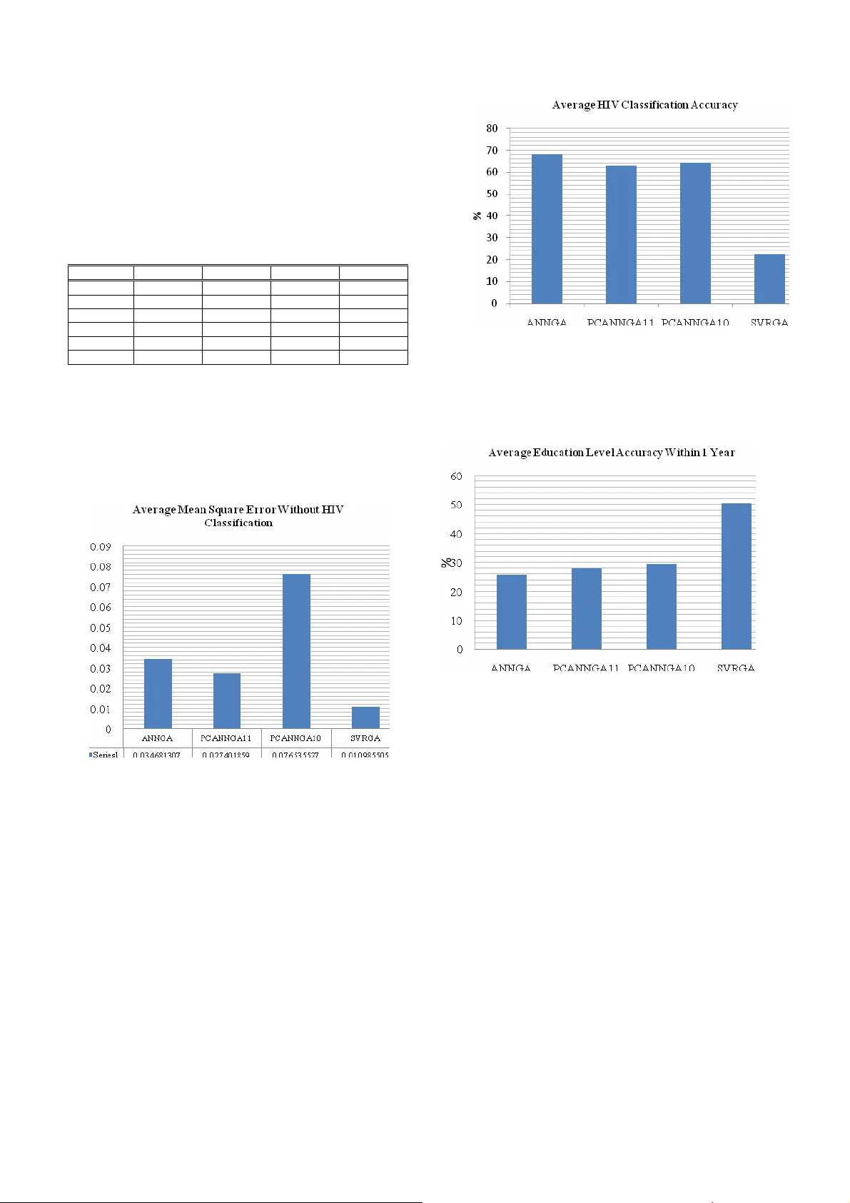
Autoencoder, Pr incipal Component A nalysis and Supp ort Vector Regre ssion for Data Imputation Vukosi N. M arivate*. F ulufhelo V. Nelwamodo** Tshilidzi Ma rwala*** Schoo l of Electrical and In formation Engineering , University of the Witwatersrand, Johannesbu rg, 2050, South Africa *(e-mail: vuk osi.marivate@stud ents.wits.ac.za). **(e-mail: f.n elwamondo @ee.wits.ac.za). *** (e-ma il: tshilidzi.mawala@wits.a c.za). Abstract: Data collection often results in records that have missing values or variables. This investigatio n compares 3 different data imputation models and identi fies their m erits by using accurac y measures. Autoencoder Neural Networks, Principal components and Suppor t Vector regression ar e used for prediction and combined with a genetic algor ithm to then i mpute missing variables. The use of PCA improves t he o verall per formance o f the autoe ncoder network while the use of suppo rt vector regressio n shows pro mising potential for future investigation. Accuracies o f up to 9 7.4 % on imput ation of some of the variables were ac hieved. 1. INTRODUCT ION Acquired immunodeficienc y syndro me (AIDS) is a collectio n of symptoms and infections resulting from the specific damage to the immune system caused by the human immunodeficiency vir us (HIV) in humans (Marx, 198 2). South Africa has seen an increase in HIV infection rates in recent years as well as ha ving the highest number o f peo ple living with the virus. This results fro m the high pr evalence rate as well a s re sulting deaths fro m AIDS (D epartment of Health, 2000) . Research into the field i s thus strong and ongoing so as to tr y to identif y ways into dealing with virus in certain area s. Thus de mographic da ta is used o ften to cla ss people living with aids a nd how they are a ffected. Thu s proper data collection needs to be done so as to understand where a nd ho w the virus is spread ing. This will give more insight into ways in whic h education and a wareness can be used to eq uip t he Sout h African po pulation. B y be ing ab le to identify factors t hat dee m certain people or populations i n higher ris k, the gover nment c an then deplo y strategies an d plans within those areas so as to help the peop le. The problem with data collection in surveys is that is suffers from information los s. This can result from incorrect data entry or a n un filled fie ld in a surve y. T his inve stigation explores the field of d ata imputation. The app roach taken is to use regression models to model the interrelationship s between data variables and then underta ke a c ontrolled and planned appro ximation of da ta using the regres sion m od el and an optimisation mod el. Data i mputation using Auto Encoder Neural Net works as a regressio n m odel has bee n carried out by Abdella and M ar w ala (Mussa et al , 2005) and others (Leke et al , 20 05) ( Nelwamondo et al, 200 7a ) while other variations are available in literature includin g Expectation Maximi sation ( Nelwamondo et al, 2007a ) , Rough Sets (Crossin gham e t al , 2005 ) ( Nelwamondo et al, 2007b ) , Decision Trees ( Barcena et a l , 2002). T he use of Auto Encoder Net works comes with the price of computational complexity and a time trade-off as a disadvantage that is mostl y cit ed for the use of other method s (Nelwamondo et al , 2007b), . The advantage o f using Auto Encoder Networks it the h igh level of accuracy. The data used in th is investigatio n is H IV de mographic data co llected from ante-natal clinic s from around Sout h Africa. This report focuses on i nvestigating the use of dif ferent regression methods that of fer a glance into the data imputation world. The repo rt fir st gives a b ackground int o missing data, neural netwo rks and the o ther regres sion methods used. Secondly the data set to b e used is intro duced and explained. The methodology is give n and then ca rried through. B y t he end of the r eport the results ar e gi ven and then discussed. 2. BACKGROUND 2.1 Missing Da ta Data collection for ms the b ackbone of most pro jects and applications. T o ac curately use the data all infor mation required must b e a vailable. Data collectio ns suf fer from missing values/data variables. This for example can be in the form of unfilled fields in a surve y or data entry mistakes. Simply removi ng all entries c oncerned with the missing value is not always the b est so lution. There are three dif ferent t ypes of missing data mechanisms as discussed by Little and Rubin (Little et al , 200 0). • Missing Co mpletely at Rand om ( MC AR ) – This is when t he pr obability of t he missing val ue o f a variable x is unrelated to itself or any other variab les in the data set. • Missing at Random ( M AR ) – T his implies t hat t he probabilit y of missing d ata of a particular variable x depends on other variables but not itsel f • Non-ignorable – T his is when the missing value o f variable x dep ends on itself e ven t hough o ther variables are kno wn Methods a re need ed to i mpute the missing data. T here a re numerous ways that ha ve b een u sed to impute missing dat a. The approac h take n in th is i nvestigatio n is to use re gression methods to find the inter-relationships between the d ata and then u se t he r egression methods to veri fy the approxi mations that a re made. T he next subsections discu ss the different regression methods used. 2.2 Neural Networks Neural Net works are co mputational models that have the ability to learn and model s ystems. T hey have the abilit y to model non-linear syste ms (Bishop, 1995). T he neural network architecture used is a multilayer percep tron network (Bishop, 1 995) as shown in Fig. 1 . Fig. 1 MLP Neural Net work This has two layers of weights which con nect t he i nput layer to the output layer. The middle of the net work i s made up o f a hidden layer. This layer can be made up of a different number of hidden nodes. This number ha s to b e opti mised so that t he network can model systems b etter (Krose et a l , 1996). An increase i n hidden nodes translates into an i ncrease in t he co mplexity of t he s ystem. The output and the hidden nodes also have activatio n functions (Bishop , 1995 ). T he general eq uation of a MLP neural network i s sho wn below (1): ) ) ( * ( 1 1 ) 2 ( 0 ) 1 ( 0 ) 1 ( ) 2 ( ∑ ∑ = = + + = M j d i k j ji inner kj outer k w w w f w f y (1) The activation function ( Fo uter ) chose n for the project was linear. The i nner activation ( Finner ) function c hosen was the hyperbolic tangent f unction (tanh). This ser ved to increase accuracy in regression (Kr ose et al , 1996) . T his functi on produced the best res ults dur ing training. T hus the relation becomes (2): ∑ ∑ = = + + = M j d i k j ji kj k w w w w y 1 1 ) 2 ( 0 ) 1 ( 0 ) 1 ( ) 2 ( ) tanh( * (2 ) For this p roje ct the Netlab ( Nabney, 2001) MATLAB toolbox w as utilised. T he Netlab to olbox was used to implement the neural networks. 2.3 Au to-encoder Networks Autoencoder/ Auto Associativ e neural networks are neural networks t hat are trained to recall their inputs. T hus th e number of inputs is equa l to the number of outputs. Autoencoder neural net works have a bo ttleneck t hat r esults from the structure of the hidden nodes (Thompson et al. , 2002). T here are less hidden nod es than i nput nodes. T his results in a butter fly structur e. The autoencoder net work is preferred in recall applications as it ca n map l inear a nd nonlinear relationships be tween all of the i nputs. T he autoencoder struct ure results in the co mpression of da ta into a smaller d imension and t hen dec ompressing i nto the outp ut space. Autoencoder s have been u sed in a number of applications incl uding missi ng d ata imputatio n (Mussa & Marwala, 2005 ) (Nelwamondo et al , 2007a). In this i nvestigation an auto encoder networks was constructed using the MLP structure discus sed i n the previous s ubsection. The H IV da ta was fed into the net work and the networks was tr ained to recall t he input s. Thus the structure is as in Fi g. 2: Fig. 2. Autoencod er Neural Net work 2.4 Support V ector Regression Support Vec tor Machi nes are a s upervised learning method used mainly for clas sification. Support vector machines are classifiers d erived fro m statis tical lear ning theor y and were first intro duced by Vapnik (1998). They have also been extended to regres sion thus r esulting i n the ter m Support Vector Regression (SVR) (Gunn, 1997) . In suppor t vecto r regression the input x is ma pped to a higher dime nsional feature spa ce Φ ( x ) in a non li near manner. T his is depicted by (3) where b is the t hreshold for the suppo rt vector equation. b x w x f + Φ ⋅ = )) ( ( ) ( (3) w and b are constants a nd can b e estimated by reducing t he empirical risk and a co mplexit y term. The above equation is for a li near app roximation of a function. )) ( ( x w Φ ⋅ describes the dot pro duct between w and ) ( x Φ . In (4) b elo w the first term i s the e mpirical ris k and t he second ter m represents the co mplexity. 2 1 2 ) ) ( ( ] [ ] [ w y x f C w f R f R i Z i i emp reg λ λ + − = + = ∑ = (4) The reduction of (4) is subject to the minimisation of the complexity as well as the optimisation o f the reg ularisation parameter λ . T he constant λ >0 d etermines the trad e-off between the flatness of f and the a mount up to w hich deviations la rger than ε are to lerated. C is the cost functio n. Z is the number o f records in the training set. By introducing ε term the n modelling non li near functions ca n be done. T he non li near m odelling can b e a t ver y high dimensions a nd can take lo ng to co mpute solutions. T o m ake the co mputation easier kernel f unctions are used (Gunn, 19 97). T here are numerous kernel functions and the one e mployed in t he investigation is the Rad ial b asis Functio n kernel. For an in depth tutor ial on support vec tor machines for cla ssification and regression see the tutorial by Gunn (1997). The least squares supp ort vector toolbox was us ed for the in vestigation (Suykens et al, 20 02). 2.5 Princip al Componen t Analysis Principal component analysis (PCA) (Shlens, 2005)is a statistical technique that is co mmonly used to find patter ns in high di mensional d ata ( Smith, 2002). The d ata c an then b e expressed in a way t hat highlig hts its si milarities a nd differences. Another propert y is that, a fter finding the patterns in t he data the da ta can t hen be compressed without much data loss. This is adv antageous for ANNs as it will result in a r eduction of t he number of nodes needed, thus increasing computatio nal speeds. A principal co mponent analysis take s place i n the follo wing manner. First da ta is taken a nd t he mean o f each d imension is subtracted from the data. Sec ondly the covarian ce matrix of the da ta is then calculated. Thirdly t he eige nvalues and ei genvectors o f the covariance matrix are calculated. The highe st eigen value correspo nds to the eigenvector that is the pr incipal component. This is where the notion of data compressio n then comes in. Using the chosen eigenvectors the dimension of the data can be r educed while retaining a large amou nt of information. B y using only the largest eige nvalues and their correspo nding eigenvectors co mpression can be used as well as a simple transformation. T hus the data compression or transformation is (5 ): PC D P × = (5) Where D is the o riginal data set, PC is the principa l component matrix a nd P is the transfor med data. The principal co mponent a nalysis multiplication results i n a data set that emphasises the r elationships bet ween t he data whether smaller o r the same dimension. T o return to the original data the follo wing equation i s used (6) : 1 ' − × = PC P D (6) Here D’ is the retr ansformed data. I f all of the principal components are used from the co variance matrix then D = D’ . T he transfor med data ( D ) can be used in conj unction wit h the ANN to increase the e fficiency o f t he ANN by reducing its complexity (number of training c ycles). These resu lts from the prop erty of the P CA extracti ng linear r elationshi ps between the d ata variable s, thus the ANN only needs t o extract the non linear relationships. This t hen results i n less training c ycles that are neede d. T hus ANNs ca n be built more efficiently. Fig. 3 illustrates this c oncept. T he P CA functio n in Netlab was used for the investiga tion 0. Fig. 3. PCA Autoencod er Neural Network 2.6 Gen etic Algorithms Genetic algorith ms ar e define d as po pulation based models that u se s election and reco mbination operato rs to g enerate new sample poi nts in search space (Whitley, 19 94). Genetic algorithms are primarily use d for optim isation a s the y ca n find values f or variab les that w ill achieve a tar get. In this investigation the genetic a lgorithm is used to find the input into regress ion model that will result in the m ost accurat e missing data value. Ge netic algorithm use is goo d for non linear functions and applications, thu s the use in this investigation. The o verview of the proced ure of genetic algorithm is the same as t hat of natural selection. A ge netic al gorithm starts with a creatio n of a random population o f “chro mosomes”. T hese chro mosomes ar e normally in binary format. Fro m t his random population an evaluation function is used to find which of the chromoso mes is the fittest. Those who are deemed fit are then used for the selection stage. Recombination of t he c hromosomes is done by taking the f ittest chromosomes and ch oosing bits from each that will be s wapped (deemed c rossover). T his then results in a new populatio n of chro mosomes. The final stage is mutation were bits ar e the n ra ndomly c hanged within the chromosomes. From t his new pop ulation the fitness oper ation begins a gain u ntil a preset nu mber of iteratio ns. T he geneti c algorithm toolbo x was used for the investigation (Houck, 1995). 3. DATA COLLE CTION AND PRE-PROCESSING The data that is used for this investigatio n is HIV data from antenatal clinics fro m aro und South Africa. It was co llected by t he dep artment of heal th in the year 2 000. The data contains multiple input fields that res ult fro m a s urvey. T he information i s in a nu mber of different formats res ulting fro m the surve y. For exa mple the pro vinces, region and race are strings. T he age, gravidity, par ity etc. ar e i ntegers. T hus conversions are needed . T he strings were co nverted to integers by using a lookup table e. g. there are o nly 9 provinces so 1 was substituted for Gauteng etc. Data co llected fro m surveys and other d ata co llection methods normall y ha ve o utliers. T hese are normally remov ed from the data set. In t his investigatio n data set s that had outliers had only t he outlier re moved and t he data set wa s then c lassified as inco mplete. This then means that t he d ata can still b e used in the final surve y result s if the missing values are i mputed. The d ata with missin g values was not used for the training of the computational methods. T he data variables and their ranges are shown belo w in Tab le 1. Table 1. HIV Data Variab les Variable Type Range HIV Status Binary [0, 1] Education Integer 0 - 13 Age Group Integer 14 - 60 Age Gap Integer 1 - 7 Gravidity Integer 0 - 11 Parity Integer 0 - 40 Race Integer 1 - 5 Province Integer 1 - 9 Region Integer 1 - 36 RPR Integer 0 - 2 WTREV Continuous 0.638 – 1.2743 The pre-pro cessed data resulted in a reduction of trainin g data. This w as 1 2750 p rocessed data sets from around 1 6500 original recor ds in the surve y data. To use t he data for training it need s to be normalised. This ensures that t he all data variables ca n be used in trai ning. If the data is n ot normalised, so me of the data variables with larger variances will influence the result more than others. E.g. if we use WTREV and Age Gr oup data only t he age data will b e influential as it has large values. T hus all of the d ata is normalised bet ween 0 and 1. T he training data is the n split into 3 p artitions. 60 % is used for training, 15 % for validatio n and the last 25 % used for the testing stage s. 4. METHODOLOGY The appro ach taken for the pr oject is to use the regressi on methods w ith a n optimisation technique. The op timisation technique c hosen was t he Ge netic algor ithm. Fig. 4 illu strates the ma nner in which the regressio n met hods and the optimisation techniq ue will be used to impute data Fig. 4. Data i mputation Configuratio n The regression methods first had to be trained before being used for d ata imputation. T he following subsections discuss the training pro cedures for the r egression methods. 4.1 ANN Trainin g and Va lidation To train the ANN t he o ptimum number of hidd en nodes is needed. T o find it a simulation was constructed that calculated t he average error using a different number of hidden nodes. The number of hidden nodes were optimised, and found to be 10 . T his was usin g scaled co njugate gradient a linear outer a ctivation function a nd a hyperbo lic tange nt function a s t he inner activatio n function. Then the opti mal number of tr aining c ycles nee ded to be foun d. T his was do ne by a nalysing t he validation er ror as the tra ining cycles increased. This is to both avoid the possibilit y of overtrai ning the ANN a nd use t he fastest way to tra in the ANN without compromising on accuracy. It was found that 10 00 training cycles were s ufficient a s well as the use of the e arly stop ping method if t he ANN was beginning to be o ver tr ained. Validation was do ne with a data set that was not used for training. This the n res ulted in an u nbiased er ror check th at would indicate i f the network was well trained or not. 4.2 PCA A NN Training and Validation The training data was first used to e xtract t he p rincipal components. After the extractio n the trainin g da ta was multiplied with th e pr incipal co mponents and t he resulti ng data was used to tra in a ne w ANN. T his was the n labelled a PCA-ANN. T wo PCA-ANNs were trained. One PC A-ANN had no c ompression and was just a transfor m; t he oth er PCANN compressed t he d ata from 11 d imensions to 1 0. The number of hidd en node s and training cycles were opti mised as in the p revious s ubsection. The number of hidd en nodes for the PCA- ANN-11 was 10 and for the P CA-ANN-10 w ere 9. The inner a nd outer activa tion functions were as for t he ANN ab ove. Valida tion was also c arried out with an unse en data set. This a lso ensures t hat the ANN i s trained well a nd not over trained. 4.3 SVR Train ing and Valida tion To train the supp ort vector re gression model less trai ning data was needed. Only 3 000 data r ecords w ere used in this case, this was due to time co nstraints, the trai ning took a considerable amount of time on MAT LAB. E ven though a smaller training set was used the validatio n error was small. A radial basis function kernel function wa s used. The bias point and the r egularisation had to be optimised. T o op timise the t wo a genetic algorith m was utilised. T his technique has been used by Kua n-Yu Chen an d C hen-Hua W ang (Che n, 2007) w ith good results. The GA used a val idation set to fi nd the p arameters t hat resulted i n t he minimum error in a SVR regression validatio n data set. Validation was carried out after training with a n unseen set and the S VR per formed well. T his was satisfactor y and the SV R could now be used with the G A to impute missing data. 4.4 Gen etic Algorithm Configu ration The genetic al gorithm will b e configured as in the mod el in Fig. 5. Fig. 5. Genetic Algor ithm Configuratio n The inputs { are known, is unkno wn and will be found by using the r egression method and the G A. The genetic al gorithm will put a value from its initi al population into the regression model. The model will recall the value and it will b e an output. The G A will try a nd minimise the error b etween its appro ximated value and th e value that the regres sion mod el will have as an ou tput. This will be done via the fitness function o f the genetic algorit hm. The fitness e valuation functio n of a GA is normally a reduction of erro r function such as i n (7): ) ( y x e − = (7) Where x is the known value and y is the estimated value. As the GA lo cates a global maximum a nd not a minimu m equation 3 has to be changed to the form of (8): 2 ) ( y x e − − = (8) The err or thus appr oaches zer o from the negative axis a nd thus the GA will be able to find a glob al ma ximum. I n this project the genetic algorithm u ses normalised geo metric selection for selectio n, alo ng with si mple cr ossover for recombination and non uniform mutation. The GA is used t o approximate the val ues of the missing data and using t he a uto encoder net work o r the SVR mechanism then uses the evaluation functio n (9) belo w to calculate the fitness. 2                       −       − = k u k u x x f x x e (9) As ANN and the SVR are used they tr y to recall their inputs. is the unkno wn parameter t hat has just b een approxi mated by the GA while a re the known data variable s a s in Fig. 5. T he function f i s the regres sion model and is c hanged for each of th e models previousl y disc ussed. Fig. 5sho ws the co nfiguration of the GA with the regressio n methods. The GA will try and reduce the er ror bet ween the regression method and the data inputs. Thus resulti ng in a data variable that is likely to be the missing va lue. B ut fo r completeness a ll o f the outputs are used to red uce the er ror of the appro ximated value. T he regressio n methods discussed in the preced ing sect ion were co mbined with the Genet ic algorithm as in Fig. 5. This result s i n multiple data imputation mechani sms. These are the: • ANNGA(co mbination of the ANN a nd GA) • PCANNGA(co mbination of PC A, ANN and GA) • SVRGA (combinatio n of SVR and GA). The Ge netic Algorit hm w as s etup with 5 0 i nitial po pulation and 50 generation cycles. As mentioned ea rlier the GA uses simple cr ossover, geometric selection and non uniform mutation. T his pro duced the best r esults and was used for every model so as to ser ve for correct co mparisons. 5. TESTIN G The testing set f or the data imputation methods contained 1000 sets. T hese were co mplete d ata sets t hat had some of their data re moved so as to be ab le to ascertain the accura cy of the imputation methods. T he testing set is m ade up of d ata that the imputatio n methods h ave not seen yet (i.e. Data that is not part of the trai ning or valida tion set). This data was also chosen rando mly fro m the initial dataset that is o utlined in Section 3. The variab les to be imputed where chosen to be HIV status, Age, Age Gr oup, Parity and Gravidity. These were take n a s the most impor tant data variables t he need ed t o be imputed. T he testin g sets were co mprised o f 3 differen t data sets made up of a 1 000 rando m recor ds each. This offers an unbiased r esult as testing with only 1 test can have results which are the best b ut may be b iased due to the data used. 5.1 Metho ds for measuring accuracy Different measures o f acc uracy are used for the evaluati ng the e ffectiveness o f t he imput ation methods. T his is to o ffer better understa nding of the r esults. The a ccuracy measures are discussed belo w. 5.2 Mean Square Error The mean sq uare error is used for t he r egression a nd classification data. It i s used to measure the er ror between t he imputed data and t he real value data. It is expre ssed as (10): n y x e / ) ( 2 − = (10) x is the correct value data and y is the imputed data. n is the number o f recor ds in the data. T he mean sq uare er ror is calculated after the imputati on by the GA. This is befor e de-normalisation and roundin g. T hus does not carr y o ver a ny rounding error s. 5.3 Classification Accuracy For the clas sification value of the HIV d ata t he o nly acc uracy used is the n umber of cor rect hits. This mea ns t he nu mber of times the imputer imputed the correct s tatus. T his i s done after de-nor malisation and rounding. 5.4 Pred iction within Yea rs/Unit Accuracy Predictio n within year is used as a useful and eas y to understand measure of accura cy. T his for example would b e expressed as 80% acc uracy withi n 1 year for age data. This means for age data t he values that ar e found ar e 80% acc urate within a tolerance of 1 year. This m easure is used mainly for the some of the re gression data. 6. RESULTS All of t he results shown in the tables are i n percenta ges of accuracy. For HIV, Gr avidity, Parit y and Age Gap are positive match accurac y. Ed ucation L evel and Age are all accuracies with a to lerance of 1 year. 6.1 ANNGA The ANNGA was te sted with all of its optimised variabl es and trained networ k. T he results of the ANNG A dat a imputation are tabulated in Table 2 . Table 2. ANNGA Results ANNGA( %) Run 1 Run 2 Run 3 Average HIV Classification 68.9 68.6 68.0 68.5 Education Level 25.1 25.1 27.2 25.8 Gravidity 82.7 82.0 84.0 82.9 Parity 81.3 81.1 82.1 81.5 Age 86.9 86.4 85.5 82.3 Age Gap 96.6 96.0 95.4 96 The results indicate t hat the autoencod er network geneti c algorithm architect ure seems to perfor m well in the HI V classification and a s well al l the other s e xcept the educatio n level. T he high esti mation accuracies are on par with previous research. T he educatio n level seems to be the weak point. 6.2 PCANNGA The PCANNGA architec ture was run with two configurations. The first co nfiguration had no compression thus is named PCANNG A11 indicating the transformation from 11 inputs to 1 1 o utputs. T he seco nd co nfiguration has a compression of 1 value thus is named PCANNG A-10, indicating t he compression and transfor mation fro m 11 inp uts to 10 inputs . T he results of the test are shown belo w in Table 3. Table 3. P CANNGA Results PCANNGA –11 (%) Run 1 Run 2 Run 3 A verage HIV Classification 65.0 6 1.6 62.8 63.1 Education Level 27.8 2 7.3 28.2 27.8 Gravidity 87.6 8 6.5 87.1 87.1 Parity 87.5 8 6.3 87.7 87.2 Age 94.9 9 4.8 93.5 95.7 Age Gap 98.1 9 8.3 96.9 97.4 PCANNGA –10(%) Run 1 Run 2 Run 3 A verage HIV Classification 64.2 6 0.9 67.2 64.1 Education Level 27.0 3 1.3 30.2 29.5 Gravidity 86.4 8 6.3 88.2 61.0 Parity 86.2 8 6.2 87.6 86.7 Age 8.0 8.2 12.1 9 .4 Age Gap 23.9 2 0.0 24.1 22.7 The re sults for PCANNGA-1 1 indicate good estimation for all the variables except ed ucation level. PCANN GA-10 performs poor ly on Age a nd Age Gap wh ile having goo d results i n the other variables. T his results fro m the loss of information d uring t he co mpression. T his the n impacts on t he regression ability of the netwo rk r esulting in poor imputation accuracy for so me of the variables. 6.3 SVRGA The SVRGA i mputation model took a long time to run. Due to the inefficie ncies of running a co mputational such as this on MATLAB, the simulations were s low. Nonetheless the imputations d id run a nd did r eturn all re quired res ults. T he results from the SV RGA are tab ulated belo w in Tab le 4. Table 4. SVRGA Results SVRGA ( %) Run 1 Run 2 Run 3 Average HIV Classification 22.5 22.1 21.4 22 Education Level 65.4 40.3 45.6 5 0.433 Gravidity 80.9 63.2 67.4 70.5 Parity 81.4 63.3 6 6.9 70.5 Age 96.1 89.2 8 3.5 89.6 Age Gap 92.6 92.7 9 4.3 93.2 The SVRGA per forms b adly in the HI V clas sification. It performs a veragely i n t he Ed ucation le vel, Par ity a nd Gravidity. With Age and Age gap it p erforms well 6.4 Comp arison of Resu lts For the comparison of results, the pre vious accuracie s as well as t he mean square error of ea ch method will be analyse d. This will give an indicatio n of how the err ors in the imputation affect the accur acy as well a s which model produces the be st results. The average mean square er rors of the imputation methods are sho wn in Table 5 Table 5. Average Mean Square E rrors Results NN P CANN11 PCANN10 SVRGA HIV 0.269147 0.303703 0.301647 0.764407 Education 0.16663 0.13224 0.123517 0.0421 Gravidity 0.00187 0.001456 0.001478 0.003141 Parity 0.002592 0.00237 0.002373 0.004422 Age 0.001025 0.000396 0.157397 0.003178 Age Gap 0.001289 0.000548 0.097913 0.002087 In the mean square errors a s maller value is d esirable. It c an be seen fro m T able 5 that in HIV classification t he SVRG A performed t he worst as it had th e hig hest err or but in t he education level it performed the best as it has the low est error. T he follo wing figure, Fig. 6, is a graph of the a verage mean square erro r of the imputatio n models Fig. 6. Co mparison o f Average Mea n sq uare err or without HIV Classification From Fig. 6 it ca n be seen that the SV RGA has t he smalle st average mea n sq uare erro r (if HIV classificatio n is not included) from t he rest of the methods. This indicates that the SVRGA f unctioned well o n re gression par ameters and po orly on the cla ssification of HIV. The following graph in Fig. 7. makes this clea r. The A NNGA performs th e best w ith an average accurac y of 68.5 % while the rest o f the models fell behind a nd the SV RGA has t he lo west average accuracy o f 22 %. In Educatio n level accuracy t he SVRGA perfor med best. It had a n o verall accurac y o f 5 0%. This is measured within a tolera nce o f 1 year. The accuracies of the models ar e shown in Fig. 8. Fig. 8. Compariso n of Average Education Accuracy The SVR is pr edicting the ed ucation le vel better than the rest and thus is pe rforming better when co mbined with the Genetic Algor ithm to i mpute the m issing variables. The last comparison i s of t he age acc uracy. T he average accuracie s with 1 year to lerance are sho wn i n Fi g. 9 . From t he graphs it can be seen t hat the PCANN10 overall per forms po orly. As explained earlier t his res ults fro m t he d ata loss fro m th e compression of t he da ta. T he SVRGA perfor ms better than the ANNGA b ut the PCANN11 performs better than all. I n almost all of the acc uracy tests the P CANN11 per forms better than t he ANNGA thus provi ng tha t t he co mbination of the PCA a nd ANN can result i n a better i mputation method. T he PCANN11 e ven has a lo wer average mea n square error than the ANNGA as s hown in Fi g. 6. T he P CA w ithout compression has i mproved the p erformance of the ANNGA. Fig. 7. Compariso n of HIV Classificatio n Accuracy Fig. 9. Compariso n of Age Ac curacy From the compariso n o f all of the impu tation models it can be seen that t he PCANN11 p erforms better e ven though it has a worse HIV cla ssification. The SVRG A only makes go od ground on the education level and thus cannot be co nsidered superior to the P CANN11 7. DISCUSSION 7.1 Gen eral Performance The general perfor mance of the imputatio n met hods is satisfactory a nd h ighly acc urate. The high acc uracy of the imputation methods on t he v ariables makes them a v iable solution for t he Department of Health’s H IV/AIDS researc h. This aff ords researchers confidence th at the da ta collected does not have to have a lar ge a mount of it d iscarded. The ANNGA ne ural network i s stab le and the res ults were goo d. The SVRG A perfor med the best in the ed ucation leve l and this could be further investigated. T he P CANNGA11 on average shows the b est pro mise in high accuracy missin g data imputation. This res ults from its good average perfor mance in Parity, Gr avidity, Age a nd Age G ap while only la gging behind b y a small margin in the HI V clas sification and performing b etter than the ANNGA i n pred icting t he Education Le vel. Solutions with higher tolera nces tend to be given but the low to lerance used in this investigat ion was to illustrate t he high a ccuracies. Higher tolerances can be use d selectively and instead o f years in a variable li ke education levels ca n be put into 3 catego ries like p rimary sc hool, high school and tertiar y. T his has been do ne by with rou gh set theory in ( Nel wamondo et al, 20 07b ) . 7.2 SVRGA Due to t ime cons traints the supp ort vector regression c ould not be i nvestigated further. This is d ue to the fact that t he simulations of the SV RGA were very slow. SVR though is still a viable solution if a n optimised c+ + or o ther programming language toolbox is u sed instead o f a MATLAB toolbox, the speed o f co mputation will i ncrease. Thus it is suggested that more research and investigation b e done on the SVR. There have b een ca ses were the SVR has outperfor med nor mal neural networks. Thus the author believes a SVR can ou tperform an ANN. 7.3 Hyb rid A hy brid approach of u sing the ANNGA and SVRGA or PCANNGA11 and SVRGA together is al so a viable future investigation area. T his could not be implemented in the investigation d ue to time. It is expected that t his would increase the per formance o f the neural network base d methods in imputing the ed ucation level while assis ting the SVRGA in imputin g the HIV classificatio n. 7.4 Fu rther Regression vs. Classificatio n An i nvestigation into the dat a only for classi fication for the classification para meters s uch as H IV can yield b etter results. This co mes at t he price o f lo ss of ge neralisation. Leke a nd Marwala (Leke et al , 2005) investigated a classi fication based problem of HIV classification on ly. This cannot be directly used with data imputatio n witho ut then resultin g in high complexity hybrid net works with mod els onl y dea ling with missing d ata that is classification based and t hen ot her models dealing with regression b ased missing data. 8. CONCLUSION This pap er investigated and c ompared the use of 3 regressio n methods with a GA combinatio n for missing data approximation. An a utoencod er neural networ k was trained to pred ict its input space , as well as reco nfigured with a principal component a nalysis to form a principal co mponent analysis autoe ncoder neural network that predicte d the principal component tra nsformed input space. Suppo rt vector regression was a lso used in the same manner as the autoencoder network. The regression m ethods were combined with genetic algor ithms to app roximate missing data fro m a 20 00 HIV sur vey data set. The principal component autoenco der neural network genetic al gorithm model per formed the best overall, with accuracie s up to 97.4%, followed by the a utoencode r neural network genetic algorithm model. The supp ort vector regression genetic algorithm model p erformed well on approximating a m issing variable that the rest o f the models perfor med poorl y i n. T his allows for future investigatio n into hybr id s ystems wit h combinations o f the regre ssion m odels in o rder to get better results and better methods for future data imputation. REFERENCES Barcena, M.J. and Tussel, F. (200 2). Multivaria te Dat a Imputation using Trees. Documentos de Trabajo BILTOKI . 5 . Bishop, C. (19 95). Neural Networks fo r Pattern Recog nition . Oxford. K. Chen, C. Wang. ( 2007) . Suppor t Vector Regression with Genetic Algorithms forec asting to urism de mand. Tourism Manag ement. 28 , pp.215–226 . Crossingham, B. and Ma rwala, T. (20 05). Using Genetic Algorithms to Optimise Rough Set Partition Si zes for HIV Data Analysi s. ArXiv e-prints . 7 05 . Depart men t o f Health, South Africa. ( 2000) . HIV/AIDS/STD strategic plan for sout h Africa. Gunn, S.R. (19 97). Support V ector Machines for Classification a nd Regression. Technica l Report, Ima ge Speech and Intelligent Systems Research Group , University of So uthampton. Houck, C., Joines, J. and Ka y, M. (199 5) A Genetic Algorithm for Functio n Optimization: A Matlab Implementation, N CSU-IE TR, 95-09 . Krose, B . and van der Smagt, P. ( 1996) An In troduction to Neural Networks (Book Style) . Universit y of Amsterda m. Leke, B ., Marwala, T. And T ettey, T . ( 2006) Autoencod er networks for HIV classification. Current Science , 91(11) . Little, R.J. and Rubin, D.B (2 000) Statistical Ana lysis with Missing Data . 2nd Editio n. John Wiley, New York. Marx, J .L. (1982) . New disease baffles medical community. Science , 217 (4560) . 618-21 . Mussa, A., and Mar wala T . ( 2005) T he Use of Genetic Algorithms and Neural Networks to App roximate Missing Data. Database in Comp uters and Artificial Intelligence , 24(6) . Nabney, T. (2001) Netlab To olbox. Nelwamondo, F.V., M ohamed, S. and Marwala, T. (2007a) Missing Data: A Compariso n of Neural Network and Expectation Maximizatio n Techniques. Current Scien ce ( to appea r). Nelwamondo, F.V., and M arwala, T. (2007b) Rough Se ts Computations to I mpute M issing Data. ArXiv e-p rints , 704 . Shlens, J. (20 05) A Tu torial o n Principal Co mponent Analysis. Unpubli shed, Version 2. Smith, L.I. (2 002 ) A Tutorial on Princ ipal Component Analysis . Unpubli shed. Suykens, J.A.K., Van G estel, T. and De B rabanter, J., De Moor, B . a nd Va ndewalle, J. (2002 ) Least Squ ares Support Vecto r Machines . Wo rld Scientific, Singapo re. Thomson, B. B., Mar ks, R.J . and Choi, J. J. (2002). I mplicit Learning in Autoencoder Novelty Assessment. IEEE Proceeding s of the 2002 Internationa l Joint Con ference on Neural Networks , 3 , pp 2 878 – 2883. Vapnik, V. (1 998). S tatistical Learn ing Theory . W iley- Interscience, Ne w York. Whitley, D. (1 994). A Genetic Algorit hm Tutorial. Statisti cs and Comp uting. 4 , pp. 6585 .