Dualities Between Entropy Functions and Network Codes

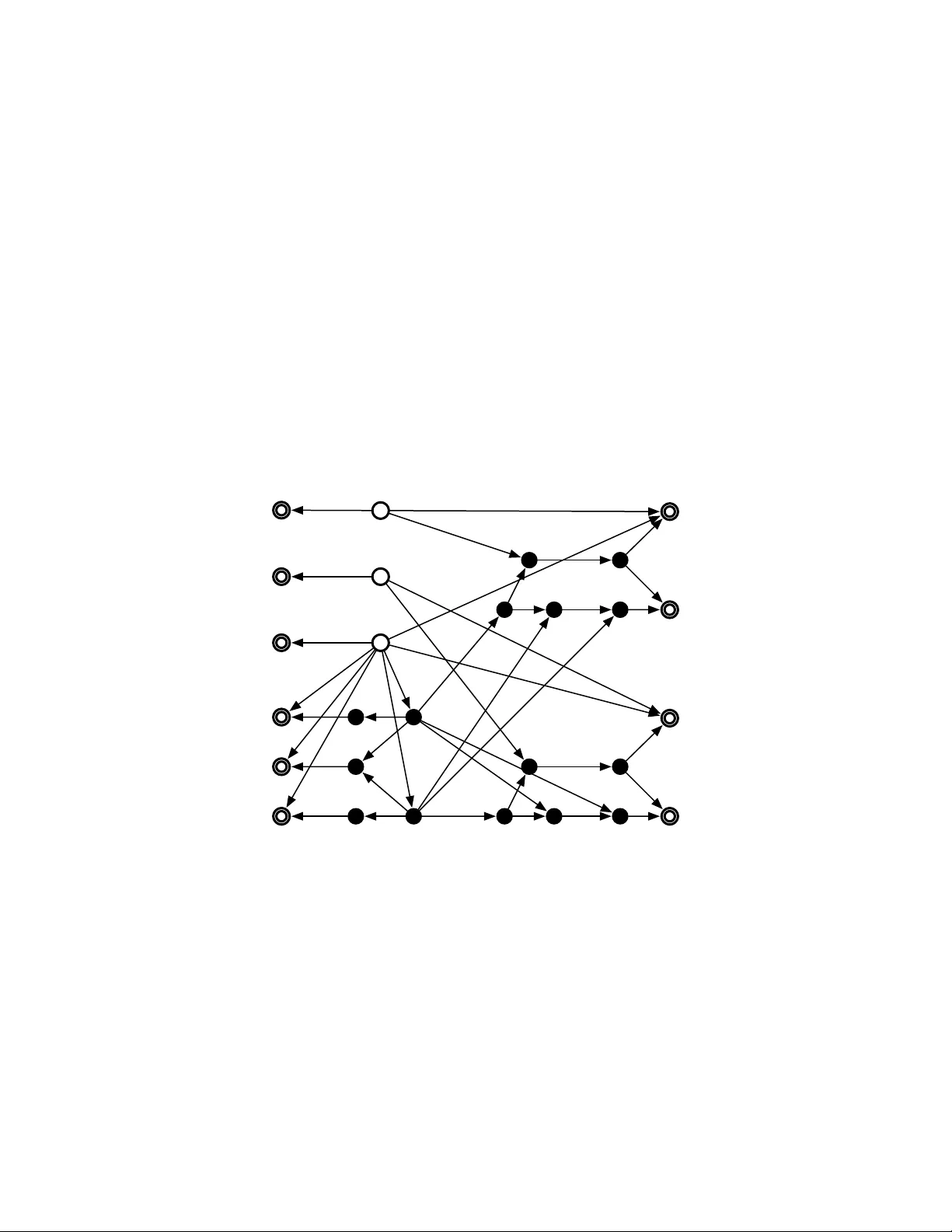
1 Dualities Between Entropy Functions and Network Codes T erence Chan 1 and Alex Grant Institute for T elecommunications Research Uni versity of South Australia, Australia { terence.chan, alex.grant } @unisa.edu.au Abstract Characterization of the set of entropy functions Γ ∗ is an important open problem in information theory . The region Γ ∗ is central to the theory of information inequalities, and as such could be reg arded as a key to the basic laws of information theory . Characterization of Γ ∗ has several important conse- quences. In probability theory , it would provide a solution for the implication problem of conditional independence. In communications networks, the capacity region of multi-source network coding is giv en in terms of Γ ∗ . More broadly , determination of Γ ∗ would ha ve an impact on conv erse theorems for multi-terminal problems in information theory . This paper provides several new dualities between entropy functions and network codes. Gi ven a function g ≥ 0 deﬁned on all proper subsets of N random v ariables, we provide a construction for a network multicast problem which is ”solvable” if and only if g is the entropy function of a set of quasi-uniform random variables. The underlying network topology is ﬁxed and the multicast problem depends on g only through link capacities and source rates. A corresponding duality is developed for linear networks codes, where the constructed multicast problem is linearly solvable if and only if g is linear group characterizable. Relaxing the requirement that the domain of g be subsets of random variables, we obtain a similar duality between polymatroids and the linear programming bound. These duality results provide an alternative proof of the insufﬁcienc y of linear (and abelian) network codes, and demonstrate the utility of non-Shannon inequalities to tighten outer bounds on network coding capacity regions. 1 T erence Chan is also with the Department of Computer Science, University of Regina. July 5, 2021 DRAFT 2 I . I N T RO D U C T I O N Information inequalities are one of the central tools of information theory . An information inequality is a relation between information measures such as entropy and mutual information that holds regardless of the speciﬁc choice of joint probability distribution on the underlying random v ariables, see [1, Chapters 12–14]. Con verse proofs inv olving chains of information inequalities are ubiquitous in the literature, extending back to Shannon. It is somewhat frustrating therefore, that a characterization of the complete set of information inequalities is lacking. Until the appearance of the Zhang-Y eung inequality [2], the only known inequalities were the so- called Shannon, or basic inequalities, being consequences of the non-negati vity of conditional mutual information (which is a special case of non-negati vity of information div ergence). Starting with [3], lar ge classes of conditional non-Shannon inequalities (e.g. contingent on imposition of certain Markov constraints) ha ve been found [4]–[7]. A countably inﬁnite class of unconstrained inequalities was reported in [8], indexed by the number of random variables N in volved (one inequality for each N ). More recently , additional unconstrained non-Shannon inequalities hav e been found [9]. Another countably inﬁnite class of unconditional inequalities was recently found in [10]. This class dif fers from [8], in that a countably inﬁnite number of inequalities were found for any ﬁxed number of N ≥ 4 random v ariables. As we shall see later , this result has profound implications. An intimately related concept is the set of entropy functions Γ ∗ . Let H [ L ] be a subset of a 2 N dimensional euclidean space. Each coordinate of this space will be index ed by a subset of a set L with N elements. Points h ∈ H [ L ] can be regarded as functions, mapping from the set of all subsets of L onto R with h ( ∅ ) = 0 . Points in H [ L ] belong to Γ ∗ if they correspond to a consistent choice of joint entropies for a set L = { X 1 , X 2 , . . . , X N } of N random v ariables. Members of Γ ∗ are called entr opic , and members of the closure of Γ ∗ , denoted by ¯ Γ ∗ , are called almost entr opic . Characterization of ¯ Γ ∗ is equiv alent to determination of the set of all possible information inequalities [1, Section 12.3]. This characterization is lacking for N > 3 . In contrast, we do kno w the set Γ ⊃ Γ ∗ corresponding to the basic inequalities. This set contains some functions that obey the basic inequalities, but are not entropy functions and do not correspond to any joint distribution on N random variables. The basic inequalities are equiv alent to the polymatroid July 5, 2021 DRAFT 3 axioms, and hence Γ is simply the set of polymatroids, implying a polyhedral structure. Characterization of Γ ∗ is an important open problem. It giv es bounds for source coding prob- lems [11]. As shown in [1], it would resolve the implication problem of conditional independence (determination of all additional conditional independence relations implied by a gi ven set of conditional independence relationships). In other ﬁelds, information inequalities are also closely linked to group theory [12] and the theory of K olmogorov comple xity [13], [14]. The focus in this paper is howe ver on the link between entropy functions and the capacity re gion of multi-source network coding. The pre vailing approach to data transport in communications networks is based on routing, in which intermediate nodes duplicate and forward packets towards their ﬁnal destination. Although such a store-and-forw ard scheme is simple to implement, it does not guarantee ef ﬁcient utilization of av ailable transmission capacity . The network coding approach introduced in [15], [16] general- izes routing by allo wing intermediate nodes to forward packets that are coded combinations of all recei ved data packets. This seemingly simple change in approach yields many beneﬁts. Not only can network coding increase throughput in multicast scenarios, it can also provide robustness to link failure [17], wiretap security [18], and minimal transmission cost [19]. Naturally , these adv antages are obtained at the expense of increased node complexity . One fundamental problem in network coding is to understand the capacity region and the classes of codes that achie ve capacity . In the single session multicast scenario, the problem is well understood. In particular , the capacity region is characterized by max-ﬂow/min-cut bounds and linear network codes are sufﬁcient to achieve maximal throughput [16], [20]. Signiﬁcant practical and theoretical complications arise in more general multicast scenarios, in volving more than one session. It was recently prov ed that linear network codes are not suf ﬁcient for the multi-source problem [20]. Furthermore, the network coding capacity region is unkno wn. In fact, there are only a few tools in the literature for study the capacity region. One po werful theoretical tool bounds the capacity region by the intersection of a set of hyperplanes (speciﬁed by the network topology and connection requirement) and the set of entropy functions Γ ∗ (inner bound), or its closure ¯ Γ ∗ (outer bound) [1], [21], [22]. Recently , these bounds have been tightened to obtain an exact expression for the capacity region, again in terms of Γ ∗ [23]. Unfortunately , the capacity region, or ev en the bounds cannot be computed in practice, due to the lack of an explicit characterization of the set of entropy functions for more July 5, 2021 DRAFT 4 than three random variables. One way to resolve this difﬁculty is via relaxation of the bound, replacing the set of entropy functions with the set of polymatroids Γ . The resulting “linear programming” bound can be quite loose. Recent work [24] based on matroid theory showed that application of the Zhang-Y eung inequality [2] yields a tighter bound for the capacity region (by obtaining a better outer bound for the set of entropy functions). The main results of this paper are ne w dualities between non-negati ve functions g ∈ H [ L ] and network codes. These duality results are based on the construction of a special network multicast problem from functions g . The underlying network topology is ﬁxed and the multicast problem depends on g only through the assignment of link capacities and source rates. Three main kinds of duality are considered, corresponding to dif ferent restrictions on g and dif ferent kinds of network codes. First, we show in Theorem 1 that the constructed multicast problem is solv able (i.e. the constructed source rates and link capacities are in the capacity region) if and only if g is the entropy function of a set of quasi-uniform random variables. This duality is extended in Theorem 2 to sho w that the multicast problem is asymptotically solv able with  error if and only if h is almost entropic. The second duality restricts attention to linear network codes. W e sho w that the multicast problem is linearly solvable if and only if g is linear group characterizable (i.e. g is an entropy function for random variables generated by vector spaces). A corresponding limiting form of this duality is also provided. Finally , by relaxing the requirement that the domain of g be subsets of random variables, we obtain a duality between polymatroids and the linear programming bound. These duality results yield sev eral immediate implications. In particular , we provide an al- ternati ve proof to [20], [24] for the insuf ﬁciency of linear (and abelian) network codes, and demonstrate the utility of non-Shannon inequalities to tighten outer bounds on network coding capacity regions. The paper is organized in the follo wing way . Section II introduces some fundamentals of network coding. Section II-A focuses on network codes with algebraic structure, and random v ariables generated by groups with a variety of algebraic structures. W e establish a relation between linear network codes and random variables generated by vector spaces and generalize this idea to deﬁne the concept of a group network code. A central theme of the paper is the trade-of f between source rate and link capacity using network coding, i.e. determination of July 5, 2021 DRAFT 5 the network coding capacity region. Section II-B introduces the deﬁnitions for admissibility and achie v ability in the network coding context. Section III introduces the concept of pseudo- v ariables, which generalize random variables in such a way that allows a notational uniﬁcation of the linear programming bound with that of [21]. Section IV prov es the duality results, Theorems 1 – 5. These results rely on the construction in Section IV -A of a special network and multicast problem from a function g . Section IV -B giv es the duality between entropic functions and solv able multicast problems. Section IV -C pro vides the corresponding duality for linearly solvable multicast problems. These duality results are extended in Section IV -D to gi ve a similar link between polymatroids and the linear programming bound, i.e. a function g is a polymatroid if and only if the constructed source rates and link capacities satisfy the bound. This result relies hea vily on the notion of pseudo-variabl es introduced in Section III, and in particular on extension and adhesion of sets of pseudo-variables, discussed in Appendix I. Finally , in Section IV -E we giv e a one-way relation between the LP bound for linear codes, and polymatroids which also satisfy the Ingleton inequality . Section V explores the implications of our results, which include the insuf ﬁciency of linear or ev en (abelian) group network codes, and the necessity for non-Shannon inequalities for determination of the network coding capacity region. Notation: For a set A , the po wer set 2 A = {B : B ⊆ A} denotes the set of all subsets of A . Gi ven a set of |A| variables { X a , a ∈ A} , and a subset C ⊆ A , the subscript X C shall mean { X c : c ∈ C } . In contrast, the notation Y [ B ] will be used to index a single variable out of a set of 2 |A| v ariables { Y [ B ] : B ∈ 2 A } . Other notation will be introduced as necessary throughout the paper . I I . N E T W O R K S , C O D E S A N D C A PAC I T Y A directed acyclic graph G = ( P , E ) is commonly used as a simpliﬁed model of a commu- nication network. The nodes u ∈ P and directed edges e = (tail( e ) , head( e )) ∈ E respectiv ely model communication nodes and directed, error-free point-to-point communication links. The terms graph and network will be used interchangeably . For edges e, f ∈ E , write f → e as shorthand for head( f ) = tail( e ) . Similarly , for an edge f ∈ E and a node u ∈ P , the notations f → u and u → f respectiv ely denote head( f ) = u and tail( f ) = u . So far we hav e only speciﬁed the basic network topology . The communication problem is speciﬁed via imposition July 5, 2021 DRAFT 6 of a connection requirement. Deﬁnition 1 (Connection Requirement): F or any network G , a connection r equirement M = ( S , O, D ) is speciﬁed by three components representing the sessions, originating nodes and destination nodes as follo ws. S is an index set of independent multicast sessions, each of which is a collection, or stream of data packets to be multicast to a prescribed set of destination nodes. O : S 7→ P is a source-location mapping, where O ( s ) is the originating node for multicast session s . D : S 7→ 2 P is a recei ver -location mapping, where D ( s ) ⊆ P is the set of nodes requiring the data of session s . It should be noted that there is no speciﬁed rate requir ement . The connection requirement dif fers from the usual concept of multicast requirement in that it only speciﬁes whic h nodes require data from which other nodes, and not any particular desired information rate. Gi ven a connection requirement M , the goal of a network code is to efﬁciently multicast data for session s originating at node O ( s ) to all receiv ers in the set D ( s ) . Nodes are assumed to hav e sufﬁcient computing power to implement any desired network coding scheme. Let F = S ∪ E . For a network G and connection requirement M , a network code is speciﬁed by a set of source and edge alphabets {U f , f ∈ F } and a set of local coding functions Φ , ( φ e : Y f ∈F : f → e U f 7→ U e : e ∈ E ) where for ease of notation, s → e indicates O ( s ) → e , and f ∈ F : f → e means any source or edge incident to edge e . Data transmission takes place as follo ws. Session s ∈ S generates a source symbol U s , which is assumed to be independent of other sessions and uniformly distrib uted ov er U s . The link symbol transmitted along e ∈ E is U e = φ e ( U f : f ∈ F , f → e ) . In other words, the symbol transmitted along an outgoing link of a node is a function of the av ailable sources and incident link symbols. W e will refer to a network code by Φ , with the set of alphabets {U f , f ∈ F } implicitly deﬁned. Since the input and link symbols are random variables, we can also refer to the code by the set of random variables U F , where their joint distribution is implied by Φ . Clearly , H ( U S ) = X s ∈S H ( U s ) = X s ∈S log |U s | and H ( U e ) ≤ log |U e | . July 5, 2021 DRAFT 7 For a gi ven network code Φ designed for a network G with connection requirement M , the error probability P e (Φ) is deﬁned as the probability that at least one receiv er d ∈ S s ∈S D ( s ) fails to correctly reconstruct one or more of its requested source messages { U s : D ( s ) = d } . A zer o-err or network code is one for which P e (Φ) = 0 , implying that the source symbols U s are deterministic functions of the corresponding receiv er-incident edge symbols. A. Algebr aic network codes The abov e formulation imposes no restriction on the choice of alphabets and local coding functions. Ho wev er , in practice, it may be preferable to impose algebraic structure to reduce the complexity of encoding and decoding. The overwhelming majority of codes studied for the point-to-point channel are in fact linear , and linear codes are also of particular interest in the network coding context. Deﬁnition 2 (Linear Network Code): A network code Φ is linear o ver a ﬁnite ﬁeld F q if all source and link alphabets U f are vector spaces over some ﬁnite ﬁeld F q , and all the local encoding functions φ e are linear . Clearly , for a linear network code, each source alphabet is a vector subspace and the symbol transmitted along link e ∈ E is a linear function of the inputs U S . As will be stated in Proposition 2, the set of all the kernels of these linear functions associated with all the links can be used to “construct” the set of source and link random variables deﬁning the network code. T o understand this relationship, we ﬁrst revie w the construction of random v ariables from a ﬁnite group and its groups [12]. Deﬁnition 3 (Construction of random variables fr om subgr oups): Suppose that U is a ran- dom variable uniformly distributed over a group G . For any subgroup G i , the set of left cosets of G i forms a partition in G . Let U i be an index set of the cosets of G i in G . W e can deﬁne a random variable U i as a function of U such that U i is the index of the coset of G i that contains U , or simply that U i is the coset of G i that contains U . The resulting random variable is said to be constructed from G and G i . Deﬁnition 4 (Gr oup char acterizable random variables): A set of random v ariables { U 1 , . . . , U N } July 5, 2021 DRAFT 8 (and its induced entropy function) is called gr oup characterizable if it is equiv alent 1 to a set of random variables constructed from a ﬁnite group G and its subgroups G 1 , · · · , G N . If G is abelian, then { U 1 , · · · , U N } (and the entropy function) is called abelian gr oup char ac- terizable . If in addition G and G 1 , · · · , G N are all vector spaces, then the set of random v ariables (and the entropy function) is called linear gr oup char acterizable . Denote the set of group characterizable entropy functions by Γ ∗ G ⊂ Γ ∗ , the set of abelian group characterizable functions by Γ ∗ ab and the set of linear (with respect to a ﬁnite ﬁeld F q ) group characterizable functions by Γ ∗ L ( q ) . Then, it is clear that Γ ∗ L ( q ) ⊂ Γ ∗ ab ⊂ Γ ∗ G ⊂ Γ ∗ . Random v ariables constructed from subgroups ha ve been shown to ha ve many interesting properties. For example, suppose { U 1 , · · · , U N } is constructed from a ﬁnite group G and its subgroups G 1 , · · · , G N . Then H ( U α ) = log | G | / | T i ∈ α G i | for any non-empty subset α ⊆ N , { 1 , 2 , . . . , N } [12]. It was also proved in [12] that a linear information inequality is v alid if and only it is satisﬁed by all group characterizable random variables. Thus group characterizable random variables hav e an interesting role to play in the proof of information inequalities, Before describing some additional properties of group characterizable random v ariables, we will need the concept of quasi-uniform random variables. Deﬁnition 5 (Quasi-uniform random variable): A discrete ﬁnite random variable U deﬁned on a sample space U is called quasi-uniform if and only if it is uniformly distrib uted over its support Ω( U ) . In other words, the probability distribution of U has the following form: Pr( U = u ) =      1 / | Ω( U ) | if u ∈ Ω( U ) 0 otherwise Hence, H ( U ) = log | Ω( U ) | . Similarly , a set of random v ariables U 1 , U 2 , . . . , U N (and its induced entropy function) is called quasi-uniform if and only if e very subset of random v ariables U α , α ⊆ { 1 , 2 , . . . , N } is quasi-uniform, i.e. H ( U α ) = log | Ω( U α ) | . 1 T wo sets of random v ariables { U 1 , · · · , U N } and { V 1 , · · · , V N } with probability distributions P U and P V respectiv ely are “equiv alent” if for each i = 1 , · · · , N , there is a one-to-one mapping τ i from the support of U i to the support of V i such that P U ( U 1 , · · · , U N ) = P V ( τ 1 ( U 1 ) , · · · , τ N ( U N )) . In this paper , two sets of equiv alent random v ariables will be regarded as identical. July 5, 2021 DRAFT 9 Lemma 1 ( [12], [25]): Random v ariables induced by groups and subgroups are quasi-uniform. Hence Γ ∗ L ( q ) ⊂ Γ ∗ ab ⊂ Γ ∗ G ⊂ Γ ∗ Q ⊂ Γ ∗ where Γ ∗ Q is the set of all quasi-uniform entropy functions. W U 1 U 2 U 2 U 1 Fig. 1. The side-information network. Lemma 2: W ith reference to Figure 1, consider a simple coding problem in which there is a transmitter (indicated by an open circle) and a recei ver (indicated by a double circle) connected by a noiseless point-to-point link. A source U 1 is av ailable at the transmitter , while correlated side-information U 2 is av ailable at both transmitter and receiv er . The coding problem is to encode U 1 , U 2 into a symbol W deﬁned on the sample space W such that U 1 can be constructed perfectly at receiv er from W and U 2 . Suppose that { U 1 , U 2 } is quasi-uniform. Then one can have a zero-error code with rate log | Ω( U 1 , U 2 ) | / | Ω( U 2 ) | = H ( U 1 | U 2 ) , where the code rate is deﬁned as log |W | . Pr oof: Since U 2 is av ailable to both transmitter and receiv er , U 1 can be reconstructed perfectly if the transmitter only sends the index of u 1 in the set { u 1 : ( u 1 , u 2 ) ∈ Ω( U 1 , U 2 ) } for any giv en u 2 ∈ Ω( U 2 ) . By the quasi-uniformity of { U 1 , U 2 } , the cardinality of the set { u 1 : ( u 1 , u 2 ) ∈ Ω( U 1 , U 2 ) } is | Ω( U 1 , U 2 ) | / | Ω( U 2 ) | for any u 2 ∈ Ω( U 2 ) . Hence, one can easily construct a zero-error code at a rate of log | Ω( U 1 , U 2 ) | / | Ω( U 2 ) | = H ( U 1 | U 2 ) that solves the coding problem. If the group and subgroups in question possess additional algebraic properties, the induced random variables may also satisfy certain additional properties. One interesting example, prov ed in [26], [27] is giv en as follows. July 5, 2021 DRAFT 10 Pr oposition 1 (Ingleton’ s inequality): Suppose that the set of random v ariables { U 1 , . . . , U N } is abelian group characterizable. Let { V 1 , V 2 , V 3 , V 4 } ⊆ { U 1 , . . . , U N } . Then g (1 , 2) + g (1 , 3) + g (1 , 4) + g (2 , 3) + g (2 , 4) ≥ g (1) + g (2) + g (3 , 4) + g (1 , 2 , 3) + g (1 , 2 , 4) (1) where g ( α ) , H ( V α ) . Pr oposition 2: Suppose that a set of random variables { U f , f ∈ F } deﬁnes a zero-error linear network code. Then { U f , f ∈ F } is linear group characterizable. Pr oof: [Proof Sketch] Suppose that Φ = { φ e , e ∈ E } is a zero-error linear network code with inputs U s ∈ U s for s ∈ S and link symbols U e ∈ U e for e ∈ E . W e will now construct a linear group characterization for the set of source/link random variables induced by Φ . Let 1) G be the vector space formed by the Cartesian product of Q s ∈S U s ; 2) ψ s : G 7→ U s be a linear function such that ψ s ( U s : s ∈ S ) = U s ; 3) ψ e : G 7→ U e be a linear function such that U e = ψ e ( U s : s ∈ S ) ; ( This is possible as all local coding functions φ e ar e linear ) 4) G f is the kernel of ψ f , denoted by ker( ψ f ) , for f ∈ S ∪ E . Hence, G f is a subspace of G . Then it is straightforward to sho w that for any ( U s : s ∈ S ) and f ∈ F , the value of ψ f ( U s : s ∈ S ) can be uniquely determined from the index of the coset of G f that contains ( U s : s ∈ S ) and vice versa. In other words, the link random v ariable U f is equi v alent to the one induced by the subspace G f . A natural interpretation of Proposition 2 is that linear network codes are those codes whose induced source and link random v ariables can be characterized by a vector space and its subspaces. Dev eloping this line of thought more generally , we make the follo wing deﬁnition. Deﬁnition 6 (Gr oup network code): A gr oup network code is a network code { U f , f ∈ F } whose source and link random variables are induced by a ﬁnite group G with subgroups G f , f ∈ F . Furthermore, a group network code is called abelian if G is abelian. For a group network code Φ = { U f , f ∈ F } , encoding at intermediate nodes works as follows. Suppose that the source and link random variables { U f , f ∈ F } are characterized by a ﬁnite group and its subgroups G f for f ∈ F . For any f ∈ F , let U f be the index set for the set of left cosets of G f in G . Each edge e receives symbols { U f : f → e } , which are indexes of cosets G f in G . The symbol U e to be transmitted along edge e is the index of the left coset G e that contains the intersection of the cosets of G f index ed by { U f : f → e } . July 5, 2021 DRAFT 11 In fact, in the special case when the group and all its subgroups are vector spaces, we can index the coset of G e as elements in a vector space such that U e is indeed a linear function of { U f : f → e } . Example 1: An R -module generalizes the concept of vector space, where the scalars are a members of a ring R , instead of a ﬁeld. It consists of an abelian group K , and an operation of left multiplication by each element in R . In particular , for all r , s ∈ R and g , h ∈ K , r g ∈ K ( r s ) g = r ( sg ) ( r + s ) g = r g + sg r ( g + h ) = r g + r h 0 g = 0 . R − modul e codes hav e been proposed as generalizations of linear network codes [20]. Messages to be transmitted along edges are elements in K . The only difference is that local encoding functions must be of the form U e = X f ∈F : f → e r f e U f where r f e ∈ R . As such, there exists elements M es ∈ R such that U e = X s ∈S M es U s . Let G be the |S | -fold Cartesian product of K . For all e ∈ E and s ∈ S , let G e = ( ( U s ∈ K : s ∈ S ) : X s ∈S M es U s = 0 ) G s = { ( U s ∈ K : s ∈ S ) : U s = 0 } . Then it is straightforward to sho w that G f is an abelian subgroup of G for f ∈ F and that the source and link random variables induced by the R − modul e code is characterized by the subgroup G and its subgroups G f , f ∈ F . July 5, 2021 DRAFT 12 B. The sour ce rate-link capacity tradeoff So far , we have only considered networks, and codes designed to meet particular connection requirements. T ypically howe ver , each link has limited capacity , and a fundamental design consideration is the tradeoff between supportable network throughput and link capacities. Of primary interest is determination of the minimal link capacities ω , ( ω e : e ∈ E ) required to transmit sources ov er a network at giv en rates λ , ( λ s : s ∈ S ) such that all receiv ers can reconstruct their desired messages with no, or arbitrarily small probability of error . Deﬁnition 7 (Admissible rate-capacity tuple): Given a network G = ( P , E ) and a connection requirement M , a rate-capacity tuple ( λ, ω ) is admissible if there exists a zero-error network code Φ = { U f , f ∈ S ∪ E } , such that H ( U e ) ≤ log |U e | ≤ ω e , ∀ e ∈ E , H ( U s ) = log |U s | ≥ λ s , ∀ s ∈ S , where U e is the message symbol transmitted along link e and U s is the input symbol generated at source s . Coding ov er long block of symbols often improves the rate of point-to-point codes. Similarly , increased efﬁcienc y may be expected for network codes operating ov er a long block of source symbols. Therefore, we also consider the asymptotic tradeoff between source rates and link capacities. Deﬁnition 8 (Asymptotically admissible): A rate-capacity tuple ( λ, ω ) is asymptotically ad- missible if there exists a sequence of zero-error network codes Φ ( n ) = { U ( n ) f , f ∈ S ∪ E } and positi ve normalizing constants r ( n ) such that lim n →∞ 1 r ( n ) H  U ( n ) e  ≤ lim n →∞ 1 r ( n ) log |U ( n ) e | ≤ ω e , ∀ e ∈ E , lim n →∞ 1 r ( n ) H  U ( n ) s  = lim n →∞ 1 r ( n ) log |U ( n ) s | ≥ λ s , ∀ s ∈ S . The above two deﬁnitions consider zero-error network codes. Relaxing the requirement to allo w arbitrarily small error probability prompts the following deﬁnition. Deﬁnition 9 (Achie vable rate-capacity tuple): A rate-capacity tuple ( λ, ω ) is achie vable if there exists a sequence of network codes Φ ( n ) , { U ( n ) f , f ∈ S ∪ E } and positi ve normalizing July 5, 2021 DRAFT 13 constants r ( n ) such that lim n →∞ 1 r ( n ) H  U ( n ) e  ≤ lim n →∞ 1 r ( n ) log |U ( n ) e | ≤ ω e , ∀ e ∈ E , lim n →∞ 1 r ( n ) H  U ( n ) s  = lim n →∞ 1 r ( n ) log |U ( n ) s | ≥ λ s , ∀ s ∈ S , lim n →∞ P e  Φ ( n )  = 0 . Assuming that the underlying network and connection requirement are known implicitly , the set of admissible, asymptotically admissible and achiev able rate-capacity tuples will be denoted Υ 0 , Υ ∞ and Υ  respecti vely . The preceding deﬁnitions place no restriction on the class of network codes under considera- tion. Ho we ver , if a rate-capacity tuple is admissible/asymptotically admissible/achie v able using a network code in a speciﬁc class C (e.g. the class of linear network codes), then that rate-capacity tuple is said to be admissible/asymptotically admissible/achiev able by network codes in C , and the corresponding sets are denoted Υ 0 C , Υ ∞ C and Υ  C . In this paper , we are interested in two special classes of netw ork codes, (i) linear network codes (with respect to an underlying ﬁnite ﬁeld F q ) and (ii) abelian group network codes. The sets of admissible/asymptotically admissible/achiev able rate-capacity tuples by linear network codes are respecti vely denoted by Υ 0 L ( q ) , Υ ∞ L ( q ) and Υ  L ( q ) . Similarly , the set of admissible/asymptotically admissible/achie vable rate-capacity tuples by abelian group network codes are respectiv ely de- noted by Υ 0 ab , Υ ∞ ab and Υ  ab . Discov ering the hidden structure of these sets of rate-capacity tuples is the key to understanding the tradeoff between source rates and edge capacities. In the follo wing, we list some basic structural properties of Υ 0 C , Υ ∞ C and Υ  C when C is either the class of all network codes, linear network codes or abelian group network codes. P1) The sets Υ 0 C , Υ ∞ C and Υ  C are closed under addition. In other words, if tuples ( λ, ω ) and ( λ 0 , ω 0 ) are in Υ 0 C (or respectiv ely in Υ ∞ C and Υ  C ), then the element-wise addition of the two tuples will still be in the same set. P2) Υ ∞ C and Υ  C are closed con ve x cones, and con(Υ 0 C ) = Υ ∞ C where con(Υ 0 C ) is the minimal closed con ve x cone containing Υ 0 C . P3) Admissibility implies asymptotic admissibility which further implies achie vability , Υ 0 C ⊆ Υ ∞ C ⊆ Υ  C . July 5, 2021 DRAFT 14 I I I . P S E U D O - V A R I A B L E S A N D B O U N D S The sets of admissible/achiev able rate-capacity tuples are difﬁcult to characterize explicitly . In fact, we will sho w later that ﬁnding these sets is at least as hard as determining the set of entropy functions Γ ∗ . Due to the difﬁculty of the problem, results on characterizing the set of achiev able rate-capacity tuples are quite limited [21], [24], [28], [29]. While inner bounds and outer bounds constructed with entropic/almost entropic functions exist [1], these bounds are not computable and hence are of limited practical use. The only known computable outer bound is the Linear Programming (LP) bound, which is constructed using polymatroids [1]. The remainder of this section provides a brief re view of these bounds. W e use the opportunity to introduce notation (dif fering slightly from the original manuscripts), facilitating later discussion. Let L be a nonempty ﬁnite set. Recall that H [ L ] (or simply H ) is a real euclidean space which has 2 |L| dimensions and coordinates index ed by the set of all subsets of L and that g ( ∅ ) = 0 for all g ∈ H [ L ] . Speciﬁcally , if g ∈ H , then its coordinates will be denoted by ( g ( A ) : A ⊆ L ) . W e call L a ground set. Each g ∈ H can also be viewed as a real-v alued function g : 2 L 7→ R deﬁned on each subset of L . Deﬁnition 10 (P olymatr oid): A function g ∈ H [ L ] is a polymatr oid if it satisﬁes g ( ∅ ) = 0 (2) g ( A ) ≥ g ( B ) , if B ⊆ A non-decreasing (3) g ( A ) + g ( B ) ≥ g ( A ∪ B ) + g ( A ∩ B ) submodular (4) Note (2) and (3) imply non-ne gati vity of a polymatroid. Let L be a set of discrete random v ariables with ﬁnite entropies. Note that L contains random variables rather than indexes for a set of random variables. This induces a function g ∈ H where g ( A ) is the joint entropy of the set of random variables ∅ 6 = A ⊆ L . Functions so-deﬁned will be called entr opy functions . It is well-kno wn that entropy functions are polymatroids ov er the ground set L . In fact, in the context of entropy functions, the polymatroid axioms are completely equi valent to the basic information inequalities (i.e. non-negati vity of conditional mutual information) [1, p. 297]. It is by now well-kno wn ho we ver that there are other information inequalities that are not implied by the polymatroid axioms. The set of entropy functions is denoted Γ ∗ , while the set of polymatroids is Γ . While an entropy function takes a subset of random variables as argument, a polymatroid g July 5, 2021 DRAFT 15 more generally takes a subset of the ground set L as ar gument, where the elements of L may or may not be random variables. For simplicity , we shall call the elements of the ground set of a polymatroid pseudo-variables . They differ from random variables in that they do not necessarily take values, and there may be no associated joint probability distribution function. It must be emphasized that pseudo-variables are only deﬁned in the context of a polymatroid g deﬁned on the ground set L . The elements of L are not pseudo-variables by themselves in the absence of an associated polymatroid. Carrying these ideas further , we will call g ( A ) the pseudo-entr opy of the set of pseudo- v ariables A , and g is a pseudo-entr opy function . T reating pseudo-v ariables as a set of basic objects associated with a polymatroid yields notational simpliﬁcation. For example, random variables are simply pseudo-v ariables possessing a probability distribution such that their pseudo-entropy function is the same as the entropy function. As such, we extend the use of H ( A ) to refer to the pseudo-entropy of a set of pseudo-variables A . Deﬁnition 11 (Entr opic function): A set of pseudo-variables (and its associated pseudo-entropy function) is called entr opic if its pseudo-entropy function is the same as an entropy function of a set of random variables. Similarly , a set of pseudo-variables (and their pseudo-entropy function) is called linear gr oup char acterizable if its pseudo-entropy function is the same as an entropy function of a set of linear group characterizable random variables. The follo wing two deﬁnitions generalize concepts of functional dependence and independence to pseudo-variables. Deﬁnition 12 (Functional dependence): Let L be a set of pseudo-v ariables. A pseudo-variable X ∈ L is said to be a function of a set of pseudo-variables A ⊆ L if H ( { X } ∪ A ) = H ( A ) . This relation will be denoted by H ( X |A ) = 0 . Deﬁnition 13 (Independence): T wo subsets of pseudo-variables A and B are called indepen- dent if H ( A ∪ B ) = H ( A ) + H ( B ) , and this relationship will be denoted by A ⊥ B . Similarly , if H ( S j ∈J A j ) = P j ∈J H ( A j ) , write ⊥ j ∈J A j . Clearly , these deﬁnitions are consistent with the usual ones used for random variables. The follo wing bound re-states the linear programming bound [1, Section 15.6] in terms of pseudo- v ariables. Deﬁnition 14 (LP bound): Gi ven a network G and a connection requirement M , the LP bound July 5, 2021 DRAFT 16 is the set of rate-capacity tuples ( λ, ω ) such that there exists a set of pseudo-v ariables { U s : s ∈ S , U e : e ∈ E } satisfying the following “connection constraint”: H ( U e | U f : f → e ) = 0 , e ∈ E H ( U s | U f : f → u ) = 0 , u ∈ D ( s ) ⊥ s ∈S U s H ( U s ) ≥ λ s , s ∈ S H ( U e ) ≤ ω e , e ∈ E . (5) Denote the set of rate-capacity tuples that satisfy the LP bound by Υ LP . From [1] it is kno wn that Υ LP ⊇ Υ  . It is interesting to notice that the use of pseudo-variables giv es a notational uniﬁcation of an inner bound and an outer bound given in [1] as follows: Pr oposition 3 (Inner and Outer bounds): Giv en a network G and a connection requirement M , let Υ in resp. Υ out be the set of rate-capacity tuples ( λ, ω ) such that there exists a set of entr opic resp. almost entr opic pseudo-variables { U s : s ∈ S , U e : e ∈ E } satisfying (5). Then Υ in ⊆ Υ  ⊆ Υ out ⊆ Υ LP . Pr oof: The proof is straightforward by rewriting the bounds obtained in [1]. Similar to the LP bound, we deﬁne the follo wing bound for abelian group network codes (including linear network codes) as follows. Deﬁnition 15 (LP-Ingleton bound): Gi ven a network G and a connection requirement M , the LP-Ingleton bound is the set of rate-capacity tuples ( λ, ω ) such that there exists a set of pseudo- v ariables { U s : s ∈ S , U e : e ∈ E } satisfying the Ingleton inequalities (1) and the connection constraint (5). Pr oposition 4: Denote the set of rate-capacity tuples that satisfy the LP-Ingleton bound by Υ LP,I . Then Υ LP,I contains Υ  ab . Pr oof: First notice that all source and link random variables of an abelian group network code must satisfy the Ingleton inequalities. The proposition then follo ws by using a similar argument as in [1] that proves Υ LP ⊇ Υ  . Since the LP and LP-Ingleton bounds are deﬁned by intersections of sev eral linear half-spaces and hyperplanes, these bounds are polyhedral. T ogether with the follo wing duality results, this implies that LP bounds are not generally tight (this is proved Section V). July 5, 2021 DRAFT 17 I V . E N T RO P Y F U N C T I O N S , N E T W O R K C O D E S A N D D U A L I T Y Gi ven a network, a connection requirement and a rate-capacity tuple, the multicast pr oblem is to determine whether or not the rate-capacity tuple is admissible or achie v able (perhaps e ven restricted to codes in a particular class). In this section, we construct multicast problems from non-negati ve functions. This construction yields sev eral dualities between properties of the generating function and the solubility of the multicast problem. W e establish three main dualities. The ﬁrst duality relates entropy functions and network codes. It can be paraphrased as follo ws. A function is quasi-uniform if and only if its induced rate-capacity tuple is admissible. This is shown in Theorem 1. Theorem 2 provides an extension which implies A function is almost entr opic if and only if its induced rate-capacity tuple is achie vable. The second duality proves similar results for linear network codes. An entr opy function is linear gr oup characterizable if and only if its induced rate- capacity tuple is admissible by linear network codes. This is Theorem 3. Again, Theorem 4 extends the result, relating almost linear group character- izable functions and achiev able rate-capacity tuples with linear network codes. The third duality , Theorem 5 relates polymatroids and the linear programming bound. A function is a polymatr oid if and only if its induced rate-capacity tuple satisﬁes the LP bound. W e also give a partial result for an e xtension to polymatroids that also satisfy the Ingleton inequality . Despite their apparent simplicity , these results leads to man y interesting corollaries: linear network codes (or more generally , abelian group network codes) are suboptimal, the LP bound is not tight, and in general the network coding capacity region is not a polytope. These consequences will be described in more detail in Section V. A. Constructing multicast pr oblems Let h ∈ H [ N ] , be a giv en non-negati ve function ov er the ground set N = { 1 , 2 , . . . , N } . The proof for the main result relies on the construction of a special network G † , a connection requirement M † and a rate-capacity tuple T ( h ) , ( λ ( h ) , ω ( h )) . July 5, 2021 DRAFT 18 Figure 2 deﬁnes the network topology , connection requirement and edge capacities. For con venience, the network is di vided into se veral subnetw orks. T o dif ferentiate the roles of network nodes, source nodes are indicated by open circles, destination nodes are double circles, and intermediate nodes are solid circles. By construction, each node takes only one role. The label beside a source node is the input message av ailable to that source node (this deﬁnes the source location mapping O ). The label beside a recei ver node indicates the desired source message to be reconstructed at that destination node (this deﬁnes the destination location mapping D ). T o simplify notation, each capacitated edge is labeled with a pair of symbols denoting the edge message (and corresponding random variable), and the edge capacity . Unlabelled edges are assumed to be uncapacitated, or to ha ve a ﬁnite but suf ﬁciently lar ge capacity (such as P α h ( α ) ) to losslessly forward all recei ved messages. The ﬁrst part of the network, shown in Figure 2(a), contains the sources. There are 2 N − 1 independent sessions, S =  S [ α ] : ∅ 6 = α ⊆ 2 N  2 . The desired source rate associated with session α is h ( α ) . Singletons { i } ∈ 2 N will be denoted without brackets, e.g. h ( i ) and S [ i ] . There are N speciﬁc edge messages that are of particular interest. Rather than naming all edge variables U e , e ∈ E , we label these N particular edge variables V j , j = 1 , . . . , N . Remaining edge v ariables will be labelled with generic symbols W , W 0 , W 00 , W ∗ and W ∗∗ . Source S [ N ] generates the network coded messages V 1 , V 2 , . . . , V N which are duplicated as required and forwarded to the rest of the network. The remaining part of the network is divided into subnetworks of three types, shown in Figures 2(b), 2(c) and 2(d). W ith reference to Figure 2(b), type 0 subnetworks connect a single source to one receiv er . There are 2 N − 1 type 0 subnetworks, indexed by the choice of ∅ 6 = α ∈ 2 N . Referring to Figure 2(c), there are 2 N − 1 type 1 subnetworks, one for each nonempty α ∈ 2 N . These subnetworks introduce an edge of capacity h ( N ) − h ( α ) between source S [ N ] and a sink requiring S [ N ] . There is an intermediate node which has another | α | incident edges (from Figure 2(a)), carrying the messages V α = { V j , j ∈ α } . The intermediate node then has an edge of capacity h ( α ) to the sink. Finally , Figure 2(d) shows the structure of the type 2 subnetworks. T ype 2 subnetworks are index ed by a set α , where ∅ 6 = α ⊂ N and an element i ∈ α, i 6∈ N . Each type 2 subnetwork 2 For simplicity , we use the same symbol to denote the index of a multicast session and the associated source random variable. July 5, 2021 DRAFT 19 S [ { i,j } ] S [ α ] S [ N ] V 1 , h (1) V 2 , h (2) V N , h ( N ) S [1] S [ i ] (a) The sources. S [ α ] S [ α ] W , h ( α ) (b) T ype 0 subnetworks S [ N ] V α { W , h ( N ) − h ( α ) S [ N ] W ! , h ( α ) (c) T ype 1 subnetworks S [ α ] S [ α ] V α { S [ N ] S [ N ] W , h ( α ) W ! , h ( N ) − h ( α ) V i V i W ∗ , h ( α ) W !! , h ( α , i ) − h ( i ) W ∗∗ , h ( α ) (d) T ype 2 subnetworks Fig. 2. The network G † . July 5, 2021 DRAFT 20 connects two sources S [ α ] and S [ N ] and two recei vers respecti vely requiring S [ α ] and S [ N ] . In addition, there are | α | + 2 other incident edges from Part 1 of the network, carrying V α and two copies of V i . For notational simplicity , we hav e written h ( α ∪ { i } ) , h ( α, i ) . So far , we hav e described a network G † , a connection requirement M † and hav e assigned rates to sources and capacities to links. Clearly M † depends only on N , and not in any other way on h . Similarly , the topology of the network G † depends only on N . The choice of h affects only the source rates and edge capacities, which are collected into the rate-capacity tuple T ( h ) . Also, we can assume without loss of generality that T ( h ) is a linear function of h . Example 2: Figure 3 shows the topology of the network G † when N = 2 . Edge labels are omitted for clarity . V 1 V 2 S [ { 1 , 2 } ] S [1] S [2] S [2] S [1] S [ { 1 , 2 } ] S [ { 1 , 2 } ] S [ { 1 , 2 } ] S [ { 1 , 2 } ] S [ { 1 , 2 } ] S [1] S [ { 1 , 2 } ] S [2] Fig. 3. The network G † when N = 2 . B. F irst Duality: Entr opy functions and network codes Theor em 1: Let h be in H [ N ] for N = { 1 , 2 , . . . , N } . The induced rate-capacity tuple T ( h ) is admissible on the network G † and connection requirement M † , if and only if h is quasi-uniform, i.e., h ∈ Γ ∗ Q ⇐ ⇒ T ( h ) ∈ Υ 0 . July 5, 2021 DRAFT 21 W e begin with a proof of the only-if statement, i.e. starting with the assumption of admissibility , we must demonstrate that the function is quasi-uniform. By Deﬁnition 7, admissibility of T ( h ) on G † , M † requires e xistence of a zero-error network code Φ with source messages S [ α ] , ∅ 6 = α ⊆ N and a subset of its coded messages V N satisfying H  S [ α ]  ≥ h ( α ) , α ⊆ N (6) H  S [ α ] : α ⊆ N  = X α ⊆N H ( S [ α ] ) (7) H ( V i ) ≤ h ( i ) , i ∈ N . (8) The remaining goal is to prov e H ( V α ) = h ( α ) for e very α ⊆ N . T o this end, we prove the follo wing series of Lemmas 3 – 8, each predicated on admissibility of T ( h ) on G † , M † . Lemma 3: H  S [ α ]  = h ( α ) for all ∅ 6 = α ⊆ N . Pr oof: Consider the type 0 subnetworks of Figure 2(b). Admissibility implies that each re- cei ver can correctly reconstruct its required source message. This is not possible unless H ( S [ α ] ) ≤ H ( W ) ≤ h ( α ) , which together with (6) proves the lemma. Lemma 4: h ( α ) ≤ H ( V α ) for all ∅ 6 = α ⊆ N . Pr oof: Consider type 1 subnetworks in Figure 2(c). In order for the recei ver to correctly determine the requested source message S [ N ] , it must be true that H ( V α ) + H ( W ) ≥ H ( S [ N ] ) . Furthermore, H ( W ) ≤ h ( N ) − h ( α ) . Hence, H ( V α ) + h ( N ) − h ( α ) ≥ H ( V α ) + H ( W ) ≥ H ( S [ N ] ) ≥ h ( N ) , where the last line follows from (6). As a result, H ( V α ) ≥ h ( α ) . Lemma 5: H ( V j ) = h ( j ) for all j ∈ N . Pr oof: A direct consequence of Lemma 4 and (8). By Lemma 5 we have taken a small step to wards our goal, establishing H ( V α ) = h ( α ) for | α | = 1 . Extension to all α will be achiev ed by induction on | α | . T o this end, the remaining lemmas take the hypothesis H ( V α ) = h ( α ) for | α | = k < N , and are proved in the context of type 2 subnetworks indexed by α and an element i ∈ N , i 6∈ α , as sho wn in Figure 2(d). July 5, 2021 DRAFT 22 Lemma 6: In type 2 subnetworks, W ⊥ S [ α ] . Furthermore, if V α = h ( α ) , then H ( V α | W , S [ α ] ) = 0 . Pr oof: By (7), S [ α ] ⊥ S [ N ] and hence H  S [ α ]  + H  S [ N ]  = H  S [ α ] , S [ N ]  ≤ H  S [ α ] , S [ N ] , W , W 0  ( i ) ≤ H ( W, S [ α ] , W 0 ) = H ( W, S [ α ] ) + H ( W 0 | W , S [ α ] ) ( ii ) ≤ H ( W , S [ α ] ) + H ( W 0 ) ≤ H ( W ) + H ( S [ α ] ) + H ( W 0 ) ( iii ) ≤ h ( α ) + H ( S [ α ] ) + H ( W 0 ) ( iv ) ≤ h ( α ) + H ( S [ α ] ) + h ( N ) − h ( α ) ( v ) = H ( S [ α ] ) + H ( S [ N ] ) . The inequality ( i ) follows from the fact that S [ N ] is determined from W, S [ α ] , W 0 at the upper recei ver in Figure 2(d). Inequality ( ii ) is by discarding conditioning (note that both W and W 0 depend on S [ N ] , so this is indeed only an inequality). Inequalities ( iii ) and ( iv ) follow from the type 2 subnetwork capacity constraints, H ( W ) ≤ h ( α ) (9) H ( W 0 ) ≤ h ( N ) − h ( α ) (10) and from Lemma 3. Finally , ( v ) is by Lemma 3. Thus the series of inequalities is actually a series of identities, and as a result, H ( W ) = h ( α ) (11) H ( W , S [ α ] ) = H ( W ) + H ( S [ α ] ) = 2 h ( α ) (12) July 5, 2021 DRAFT 23 which proves W ⊥ S [ α ] . Now consider H ( V α | W , S [ α ] ) = H ( V α , W , S [ α ] ) − H ( W , S [ α ] ) ( i ) = H ( V α , S [ α ] ) − H ( W , S [ α ] ) ≤ H ( V α ) + H ( S [ α ] ) − H ( W , S [ α ] ) ( ii ) = H ( V α ) − h ( α ) = 0 if H ( V α ) = h ( α ) where ( i ) holds since W is a function of V α , S [ α ] and ( ii ) is by (11) and (12). Lemma 7: In type 2 subnetworks, H ( W | V α , W ∗ ) = H ( W | W ∗ ) = H ( W ) , or equi v alently , I ( W ; V α , W ∗ ) = 0 . Pr oof: Recalling that i 6∈ α ⊂ N , H ( W | V α , W ∗ ) ≥ H ( W | V α , W ∗ , V i ) ( i ) = H ( W | V α , V i ) ( ii ) = H ( W | V α , V i ) + H ( S [ α ] | V α , V i , W ) = H ( W, S [ α ] | V α , V i ) ≥ H ( S [ α ] | V α , V i ) ( iii ) = H ( S [ α ] ) ( iv ) = h ( α ) ( v ) ≥ H ( W ) ≥ H ( W | W ∗ ) ≥ H ( W | V α , W ∗ ) where ( i ) follows from the fact that W ∗ is a function of V α , V i , ( ii ) follows from that S [ α ] can be reconstructed at the lo wer recei ver , and ( iii ) follows from independence of S [ α ] and ( V α , V i ) , since by (7) S [ α ] ⊥ S [ N ] and all the V j , j ∈ N depend only on S [ N ] . Finally , ( iv ) is by Lemma 3, ( v ) is by the capacity constraint (9) and the remaining inequalities simply add extra conditioning. Thus the chain of inequalities is actually a chain of identities, the last three proving the lemma. July 5, 2021 DRAFT 24 Lemma 8: In type 2 subnetworks, assuming H ( V α ) = h ( α ) , H ( W ∗ | V α ) = H ( V α | W ∗ ) = 0 . Pr oof: H ( V α | W ∗ ) = H ( V α | W ∗ , W ) + I ( V α ; W | W ∗ ) ( i ) = H ( V α | W ∗ , W ) ≤ H ( V α , S [ α ] | W ∗ , W ) = H ( V α | W ∗ , W , S [ α ] ) + H ( S [ α ] | W ∗ , W ) ( ii ) = H ( V α | W ∗ , W , S [ α ] ) ≤ H ( V α | W , S [ α ] ) ( iii ) = 0 . where ( i ) follows from Lemma 7, ( ii ) is because S [ α ] can be reconstructed at the lo wer recei ver , and ( iii ) is by Lemma 6, assuming H ( V α ) = h ( α ) . Since conditional entropies are non-ne gati ve H ( V α | W ∗ ) = 0 . (13) On the other hand, H ( W ∗ | V α ) = H ( W ∗ , V α ) − H ( V α ) = H ( W ∗ ) + H ( V α | W ∗ ) − H ( V α ) ≤ h ( α ) − h ( α ) = 0 where the last inequality uses (13), the type 2 subnetwork capacity bound H ( W ∗ ) ≤ h ( α ) and the assumption H ( V α ) = h ( α ) . Non-negati vity of conditional entropy yields H ( W ∗ | V α ) = 0 . W e are no w ready to assemble the preceding lemmas into a proof for the only-if part of Theorem 1. Pr oof: [Proof: only-if part of Theorem 1] The goal is to prove H ( V α ) = h ( α ) for all non-empty subsets α ⊆ N . This was already shown for | α | = 1 in Lemma 5. Extension to all α will be achieved using induction. First, assume the hypothesis is true for all α ⊂ N with 1 ≤ | α | ≤ k < N . For any i ∈ N and α ⊂ N such that i 6∈ α and | α | = k , consider the type 2 subnetwork of Figure 2(d). W e must show that H ( V α , V i ) = h ( α ∪ { i } ) , h ( α, i ) . By Lemma 4 we already know that H ( V α , V i ) ≥ h ( α, i ) . Therefore it remains only to prove July 5, 2021 DRAFT 25 H ( V α , V i ) ≤ h ( α, i ) . No w H ( V i , V α ) ≤ H ( V i , V α , W ∗ ) ( i ) = H ( V i , W ∗ ) ≤ H ( V i , W ∗ , W 00 ) ( ii ) = H ( V i , W 00 ) ≤ H ( V i ) + H ( W 00 ) ( iii ) ≤ H ( V i ) + h ( α , i ) − h ( i ) ( iv ) = h ( i ) + h ( α, i ) − h ( i ) = h ( α, i ) where ( i ) follo ws from Lemma 8 (which holds under the induction hypothesis), ( ii ) is due to the fact that W ∗ is a function of W 00 , V i and ( iii ) is from the subnetwork 2 capacity bound H ( W 00 ) ≤ h ( α, i ) − h ( i ) . Finally , ( iv ) is by Lemma 5. Up to this point, we hav e proved that h is the entropy function of a set of random v ariables { V 1 , . . . , V N } . T o show that h is indeed quasi-uniform, it suf ﬁces to prov e that for any subset α of N , the set of random variables V α is quasi-uniform. Since we ha ve just sho wed that H ( V α ) = h ( α ) , if the receiv er in the type 1 subnetwork can decode S [ N ] , then H ( V α | W 0 ) = H ( W 0 | V α ) = 0 . Hence, H ( W 0 ) = h ( α ) . Now according to the link capacity constraint, W 0 is deﬁned on an alphabet set of size 2 h ( α ) , and W 0 (and hence V α ) must be quasi-uniform. It remains to prov e the “if ” statement in the theorem, i.e. to show that quasi-uniform random v ariables imply admissibility . Pr oof: [Proof: if part of Theorem 1] It sufﬁces to show that one can construct a network code (deﬁned by input v ariables, and message variables) meeting the connection requirement subject to the individual capacity constraint on each link. The construction for the input variables is simple. For any ∅ 6 = α ⊆ N , deﬁne S [ α ] to be a quasi-uniform random variable with entropy h ( α ) . These input variables are also assumed to be independent. It remains to show that we can construct edge variables satisfying the capacity constraints, and which allow each recei ver to reconstruct the requested messages perfectly . By the quasi-uniformity of S [ α ] , it is clear that all receiv ers in type 0 subnetworks can reconstruct their requested message simply by having the source transmit the uncoded message, July 5, 2021 DRAFT 26 W = S [ α ] . Let { V j : j ∈ N } be a set of quasi-uniform random variables whose entropy function is h . Since H ( V N ) = H ( S [ N ] ) , there is a one-to-one mapping between Ω( V N ) and Ω( S [ N ] ) . As they are both quasi-uniform, S [ N ] and ( V j : j ∈ N ) can be regarded as the same. For type 1 networks, by quasi-uniformity of V α , one can send V α unencoded as W 0 . Then the receiv ers see V α and an auxiliary message W deﬁned on a sample space of size at most 2 h ( N ) − h ( α ) . Reconstructing S [ N ] at the recei ver is equi valent to reconstructing V N \ α at the recei ver . By the quasi-uniformity of S [ α ] and Lemma 2, V N \ α can be compressed to a symbol W of size 2 h ( N ) − h ( α ) such that V N \ α can be losslessly reconstructed from W and V α . It remains to v erify that recei vers in type 2 subnetworks can reconstruct all requested messages. Recall that both S [ α ] and V α are quasi-uniform. Assume without loss of generality that their supports are { 0 , 1 , 2 , . . . , 2 h ( α ) − 1 } . Then we can deﬁne W , V α + S [ α ] mo d 2 h ( α ) . It is easy to verify the following properties: H  W | V α , S [ α ]  = H  S [ α ] | W , V α  = H  V α | W , S [ α ]  = 0 , (14) log | Ω( W ) | = h ( α ) . (15) By (14), the upper receiv er can correctly reconstruct V α from S [ α ] and W . Using a similar compression scheme as used in type 1 subnetworks, source S [ N ] is compressed to h ( N ) − h ( α ) bits, allowing lossless reconstruction of S [ N ] at the upper receiver . On the other hand, it is easy to see that { V α , V i } is quasi-uniform. Hence V α can be compressed into W 00 with a support of size | Ω( W 00 ) | = 2 h ( α,i ) − h ( i ) such that V α can be reconstructed by using W 00 and V i . As a result, W ∗ may be transmitted as V α without any encoding. The lo wer receiv er can then recov er S [ α ] from V α and W . Since all recei vers can reconstruct their requested source messages with properly constructed message random v ariables satisfying the capacity constraints, the rate-capacity tuple T ( h ) is admissible. Deﬁnition 16: A polymatroid h is called almost entr opic if there exists a sequence of entropic pseudo-entropy functions h ( k ) and positiv e constants r ( k ) such that lim k →∞ h ( k ) /r ( k ) = h . As ¯ Γ ∗ is a closed and con vex cone [30], the set of all almost entropic functions is ¯ Γ ∗ . Theorem 1 establishes a duality , or equiv alence between the quasi-uniformity of h and admissibility of July 5, 2021 DRAFT 27 T ( h ) . The follo wing theorem extends this result to a duality between almost entropic h and asymptotically admissible (and achiev able) T ( h ) . Theor em 2: Let h ∈ H [ N ] for N = { 1 , 2 , . . . , N } and let T ( h ) be an induced rate-capacity tuple. Then we have, h ∈ ¯ Γ ∗ ⇐ ⇒ T ( h ) ∈ Υ ∞ ⇐ ⇒ T ( h ) ∈ Υ  . In other words, the rate-capacity tuple T ( h ) is asymptotically admissible (or achiev able) on the network G † and connection requirement M † if and only if h is almost entropic. Pr oof: Suppose that h is almost entropic. W e will ﬁrst sho w that T ( h ) ∈ Υ ∞ . By [12], [26], one can construct a sequence of quasi-uniform entropic functions h ( n ) and normalizing constants r ( n ) that lim n →∞ h ( n ) ( α ) /r ( n ) = h ( α ) . By Theorem 1, each T ( h ( n ) ) is admissible. By property P2, the set Υ ∞ of asymptotically admissible rate-capacity tuples is a closed and con vex cone and hence T ( h ) ∈ Υ ∞ . Clearly , T ( h ) ∈ Υ ∞ implies that T ( h ) ∈ Υ  . It remains to show that T ( h ) is achiev able implying that h is almost entropic. Suppose that T ( h ) ∈ Υ  . According to Deﬁnition 9, one can construct a sequence of normalizing constants r ( n ) and network codes Φ ( n ) with source messages { S ( k ) [ α ] , α ⊆ N } and edge messages V ( k ) N such that 3 lim k →∞ 1 r ( n ) H  S ( n ) [ α ]  ≥ h ( α ) (16) lim k →∞ 1 r ( n ) H  V ( n ) i  ≤ h ( i ) (17) lim n →∞ P e  Φ ( n )  = 0 . (18) For each v alue of the sequence index n , consider the network G † and connection requirement M † of Figure 2 with sources S = n S ( n ) [ α ] , ∅ 6 = α ∈ 2 N o and edge messages V ( n ) N . By the Fano inequality , the entropy of any source s ∈ S conditioned on the edge variables incident to any node in D ( s ) can be made as small as desired by increasing n . Follo wing a similar procedure as in the proof for Theorem 1, it can be proved that for any non-empty subset ∅ 6 = α ⊆ N , lim k →∞ 1 r ( n ) H  V ( k ) α  = h ( α ) . In other words, h is almost entropic. 3 By the Bolzano-W ierstrass Theorem which says that any sequence in a closed and bounded interval has a conv ergent subsequence, we can safely assume that lim k →∞ 1 r ( k ) H ( S ( k ) [ α ] , V ( k ) β ) exists for any nonempty subsets α, β of N . July 5, 2021 DRAFT 28 C. Second Duality: Linear gr oup char acterizable functions and linear network codes The ﬁrst duality shows that h is quasi-uniform (almost entropic) if and only if T ( h ) is admissible (achie vable). W e will now prov e a similar result, restricting the network codes to be linear . Theor em 3: Let h ∈ H [ N ] for N = { 1 , 2 , . . . , N } . The induced rate-capacity tuple T ( h ) is admissible using linear network codes on the network G † and connection requirement M † , if and only if h is linear group characterizable, i.e., h ∈ Γ ∗ L ( q ) ⇐ ⇒ T ( h ) ∈ Υ 0 L ( q ) Pr oof: [Proof: only-if part of Theorem 3] The proof of the only-if part is very similar to the one gi ven in Theorem 1. Suppose that T ( h ) ∈ Υ 0 L ( q ) , i.e., it is admissible using a linear network code Φ on the network G † and connection requirement M † . By Proposition 2, the set of induced source and link random variables by Φ is linear group characterizable. Using the same argument as in the proof for Theorem 1, h is the entropy function of a subset of these linear group characterizable random variables. Hence, h is linear group characterizable. In fact, using the same ar gument, we can sho w that if the induced rate-capacity tuple T ( h ) is admissible using abelian network codes on the network G † and connection requirement M † , then h is abelian group characterizable. Before we prove the if part of Theorem 3, we need the follo wing lemma which serv es a similar role as Lemma 2 in the proof of Theorem 1 by justifying the feasibility of certain “compression” scheme. Lemma 9: Consider a special case of the network depicted in Figure 1 where the left node recei ves T 1 ( a ) and T 2 ( a ) as inputs, where T 1 and T 2 are two linear functions deﬁned on a vector space A ov er F q . Let the kernels of T 1 and T 2 be respectiv ely B 1 and B 2 . Then, there exists a linear function W of T 1 ( a ) and T 2 ( a ) such that (1) T 1 ( a ) is uniquely determined from W and T 2 ( a ) , and (2) W takes at most q dim B 2 − dim B 1 ∩ B 2 dif ferent values. Pr oof: From B 1 and B 2 , we can construct three subspaces W 1 , W 2 and W 0 such that dim W 0 + dim W 1 + dim W 2 + dim B 1 ∩ B 2 = dim A and that for each i = 1 , 2 , the subspace B i is equal to the linear span of W i and B 1 ∩ B 2 . Hence any a ∈ A can be written uniquely as a = a 0 + a 1 + a 2 + b where a i ∈ W i for i = 1 , 2 , 3 and b ∈ B 1 ∩ B 2 . July 5, 2021 DRAFT 29 Since ker( T 1 ) = B 1 , we hav e T 1 ( a 0 + a 1 + a 2 + b ) = T 1 ( a 2 ) + T 1 ( b ) . Furthermore, one can easily construct a linear function T ∗ 1 such that T ∗ 1 ( T 1 ( a )) = ( a 2 , b ) . Similarly , there exists a linear function T ∗ 2 such that T ∗ 2 ( T 2 ( a )) = ( a 1 , b ) . T o compute T 1 ( a ) at node 2, it suf ﬁces to compute a 2 as b can be computed directly from T 2 ( a ) . A simple counting argument shows that a 2 lies in a vector subspace of dimension dim B 2 − dim B 1 ∩ B 2 . Therefore, we can set W = a 2 ov er the network and it takes at most q dim B 2 − dim B 1 ∩ B 2 dif ferent values. No w we may continue our proof for Theorem 3. Pr oof: [Proof: if part of Theorem 3] T o prov e the direct part of Theorem 3, we need to show that if h is linear group characterizable, then one can construct a linear network code (deﬁned by the induced source and link random v ariables) meeting the connection requirement subject to the individual capacity constraint on each link. Suppose that h is linear group characterizable by a vector space V and its subspaces V 1 , . . . , V N , deﬁned ov er a ﬁeld F q . Assume without loss of generality that the subspaces intersect only at the zero vector , T N j =1 V j = { 0 } . As such, h ( N ) = log q · (dim V ) and for any α ⊆ N , we ha ve h ( α ) = log q · (dim V − dim T j ∈ α V j ) . For j = 1 , . . . , N , construct linear functions f j ov er V such that k er( f j ) = V j . The source random variable S [ N ] is uniformly distributed ov er V such that the link symbols transmitted in Figure 2(a) are V j = f j ( S [ N ] ) . For any other ∅ 6 = α ⊂ N , deﬁne S [ α ] to be a random v ariable, uniformly distributed over a vector space of dimension log q 2 · h ( α ) (hence, H ( S [ α ] ) = h ( α ) ). All these source random variables are assumed to be independent. Up to this point, we ha ve described how source and link random variables are deﬁned in Figure 2(a). It remains to show that we can construct a linear network code, consisting of a set of link random variables which are linear functions of the incident source/link random variables, satisfying the capacity constraints, and which allo w each receiv er to reconstruct the requested messages perfectly . For type 0 subnetworks, all recei vers can reconstruct their requested message simply by having the source transmit the uncoded message, W = S [ α ] . Clearly , the associated link random variables in these subnetworks are linear functions of the incident ones and meet the capacity constraint. For type 1 subnetworks, let W 0 = ( V i : i ∈ α ) = ( f i ( S [ N ] ) : i ∈ α ) , which depends linearly on S [ N ] . Note that ( f i ( a ) : i ∈ α ) = 0 if and only if f i ( a ) = 0 for all i ∈ α , or equi valently , July 5, 2021 DRAFT 30 when a ∈ T i ∈ α V i . By the rank-nullity theorem, W 0 can take at most | V | / | T i ∈ α V i | different v alues. W e can thus treat W 0 as a vector in space of dimension dim V − dim T i ∈ α V i . As a result, the subnetwork can no w be treated as a special case of Lemma 9 such that T 1 ( a ) = a and T 2 ( a ) = ( f i ( a ) : i ∈ α ) . The dimensions of the kernels of T 1 and T 2 are respectiv ely 0 and dim T i ∈ α V i . By Lemma 9, the required rate is thus log q · (dim T i ∈ α V i ) = h ( N ) − h ( α ) . Similarly , for type 2 subnetworks, let W ∗∗ = ( f i ( S [ N ] ) : i ∈ α ) . As before, we can treat W ∗∗ as a vector of length dim V − dim T i ∈ α V i . Similarly , S [ α ] can also be regarded as a vector of the same length. W e can therefore deﬁne W by vector addition, W = S [ α ] + W ∗∗ . Consequently , the recei ver in the upper branch can reconstruct V α by subtracting S [ α ] from W . As before, one can ﬁnd W 0 as a linear function of S [ N ] and this function allows S [ N ] to be reconstructed from W 0 and V α . For the lower branch, we can identify a special case of Figure 1 with T 1 ( a ) = V α and T 2 ( a ) = V i . One can construct W 00 such that (1) W 00 is a linear function of T 1 ( a ) and T 2 ( a ) , (2) the kernel ker( T 1 ) = T j ∈ α V j and ker( T 2 ) = V i , and (3) the rate required is dim T j ∈ α V j − dim V i T j ∈ α V j . Therefore, we can reconstruct V α from W 00 and T 2 ( a ) where T 1 ( a ) = V α . Again, treating V α as a vector of length dim V − dim T i ∈ α V i , the recei ver at the lower branch can reconstruct S [ α ] by subtracting V α from W . So far , we have prov ed that h is linear group characterizable if and only if the rate-capacity tuple T ( h ) is admissible with a linear network code. As before, we can further generalize the result to include the case when h is almost linear group characterizable according to the follo wing deﬁnition. Deﬁnition 17: A polymatroid h is called almost linear gr oup char acterizable if there exists a sequence of linear group characterizable entropy functions h ( k ) and positiv e constants r ( k ) such that lim k →∞ h ( k ) /r ( k ) = h . It is easy to pro ve that the set of all almost linear group characterizable polymatroids is con(Γ ∗ L ( q ) ) , the minimal closed and con ve x cone containing Γ ∗ L ( q ) . Theor em 4: Let h ∈ H [ N ] for N = { 1 , 2 , . . . , N } and let T ( h ) be an induced rate-capacity tuple. Then we have h ∈ con(Γ ∗ L ( q ) ) ⇐ ⇒ T ( h ) ∈ Υ ∞ L ( q ) ⇐ ⇒ T ( h ) ∈ Υ  L ( q ) . In other words, the rate-capacity tuple T ( h ) is asymptotically admissible (or achie v able) by linear July 5, 2021 DRAFT 31 network codes on the network G † and connection requirement M † if and only if h is is almost linear group characterizable. Pr oof: Suppose that h ∈ con(Γ ∗ L ( q ) ) . By Deﬁnition 17, one can construct a sequence of linear group characterizable entrop y functions h ( k ) and positi ve constants r ( k ) such that lim k →∞ h ( k ) /r ( k ) = h . By Theorem 3, each T ( h ( n ) ) is admissible by linear network codes. By property P2, the set Υ ∞ L ( q ) of asymptotically admissible rate-capacity tuples is a closed and con vex cone and hence T ( h ) ∈ Υ ∞ L ( q ) . Clearly , T ( h ) ∈ Υ ∞ L ( q ) implies that T ( h ) ∈ Υ  L ( q ) . It remains to prove that T ( h ) ∈ Υ  L ( q ) implies h ∈ con(Γ ∗ L ( q ) ) . Suppose that T ( h ) is achie v able by linear network codes. Then one can construct a sequence of normalizing constants r ( n ) and linear network codes Φ ( n ) with source messages ( S ( k ) [ α ] , α ⊆ N ) and edge messages ( V ( k ) j , j ∈ N ) such that lim k →∞ 1 r ( n ) H  S ( n ) [ α ]  ≥ h ( α ) (19) lim k →∞ 1 r ( n ) H  V ( n ) j  ≤ h ( j ) (20) lim n →∞ P e  Φ ( n )  = 0 . (21) Similar to the proof gi ven in Theorem 2, it can be proved that for any non-empty subset ∅ 6 = α ⊆ N , lim k →∞ 1 r ( n ) H  V ( k ) α  = h ( α ) . In addition, as ( V ( k ) j , j ∈ N ) is linear group characterizable, h is almost linear group characterizable. D. Thir d Duality: P olymatr oids and the LP bound Theorem 2 provides a duality between entropy functions and network codes, namely that a function h ∈ H [ N ] is almost entropic if and only if T ( h ) is achiev able on G † , M † . As the set of almost entropic functions ¯ Γ ∗ has no explicit characterization for four or more v ariables, the sets of admissible or achiev able rate-capacity tuples are unknown. Therefore computable bounds such as the linear programming bound are of great interest. Let Γ be the set of all polymatroids. Deﬁnition 14 writes the LP bound in terms of constraints on pseudo-variables. The follo wing theorem provides a direct generalization of the ideas of the pre vious sections to pseudo-v ariables. July 5, 2021 DRAFT 32 Theor em 5: Suppose h ∈ H [ N ] . A rate-capacity tuple ( λ ( h ) , ω ( h )) satisﬁes the LP bound if and only if h is a polymatroid, h ∈ Γ ⇐ ⇒ T ( h ) ∈ Υ LP . Pr oof: The “only if ” part of the proof is a direct generalization of the proof of Theorem 1. Suppose ( λ ( h ) , ω ( h )) satisﬁes the LP bound. By Deﬁnition 14 there exists a set of pseudo- v ariables satisfying the set of (in)equalities in (5). In particular , there are pseudo-variables { S [ α ] , ∅ 6 = α ⊆ N } and V N such that H ( S [ α ] ) ≥ h ( α ) , α ⊆ N , (22) H ( S [ α ] : α ⊆ N ) = X α ⊆N H ( S [ α ] ) (23) H ( V i ) ≤ h ( i ) . (24) Follo wing the same steps as in the proof for Theorem 1 (translating random v ariables to pseudo- v ariables), shows that h is the pseudo-entropy function of V N . Hence, h is a polymatroid. T o prov e the direct part, suppose h is a polymatroid over the ground set L = { V 1 , V 2 , . . . , V N } (i.e. h is the pseudo-entropy function of V N ). W e must exhibit a set of pseudo-v ariables satisfying the set of (in)equalities (5). Whereas the proof for Theorem 1 constructs auxiliary random v ariables via data compression, we need to show how to analogously adhere auxiliary pseudo- v ariables W, W 00 etc. to the set of pseudo-variables V N . In contrast to random variables, we cannot rely on coding theorems, or other probabilistic constructions that assume the existence of an underlying probability distribution. Nev ertheless, it is possible to adhere pseudo-v ariables. This is accomplished in Appendix I, where proof of the direct part is also completed. E. F ourth Duality: Ingleton polymatr oids and the LP bound for linear codes? Finally , we can consider rate-capacity tuples which satisfy the LP-Ingleton bound of Deﬁnition 15. The following theorem establishes a relation to Ingleton polymatroids (i.e., a polymatroid satisfying Ingleton inequalities). This is sho wn in one direction only . Let Γ LP,I be the set of all Ingleton polymatroids. Theor em 6: Suppose h ∈ H [ N ] . If a rate-capacity tuple ( λ ( h ) , ω ( h )) satisﬁes the LP bound for linear codes, then h is an Ingleton polymatroid, i.e., T ( h ) ∈ Υ LP,I ⇒ h ∈ Γ LP,I . July 5, 2021 DRAFT 33 Pr oof: Suppose ( λ ( h ) , ω ( h )) satisﬁes the LP-Ingleton bound. By Deﬁnition 15 there exists a set of Ingleton pseudo-variables satisfying the set of (in)equalities in (5). In particular , there are pseudo-variables { S [ α ] , ∅ 6 = α ⊆ N } and V N such that H ( S [ α ] ) ≥ h ( α ) , α ⊆ N , (25) H ( S [ α ] : α ⊆ N ) = X α ⊆N H ( S [ α ] ) (26) H ( V i ) ≤ h ( i ) . (27) Follo wing the same steps as in the proof for Theorem 1 (translating random variables to pseudo-v ariables), shows that h is the pseudo-entropy function of V N . Hence, h is an Ingleton polymatroid. W e conjecture that the con verse of the fourth duality should also hold. In fact, it can be proved that if the con verse fails to hold, then there exists a polymatroid satisfying Ingleton inequalities but which is not almost linear group characterizable. Therefore determination of whether the con verse of the fourth duality holds is a very interesting open question. V . I M P L I C A T I O N S The results of Section IV while interesting in their own right, hav e se veral consequential applications. First, in Section V -A we consider implications to the determination of the network coding capacity re gion (in the absence of an y restriction on the class of netw ork codes). Secondly , we discuss the sub-optimality of linear network codes in Section V -B. A. The capacity r e gion Implication 1 (Har dness of a multicast pr oblem): Determination of the set of achie v able source rate-link capacity tuples Υ  is at least as hard as the problem of determining the set of all almost entropic functions. Similarly , determination of the set of source rate-link capacity tuples achiev ed by linear network codes Υ  L ( q ) is at least as hard as the problem of determining the set of all almost linear group characterizable entropy functions. Pr oof: By Theorem 2, a polymatroid h is almost entropic (and almost linear group char- acterizable) if and only if the induced rate-capacity tuple ( λ ( h ) , ω ( h )) is achie v able (with linear July 5, 2021 DRAFT 34 network codes). In other words, the problem of determining the set of all almost entropic (and almost linear group characterizable) functions can be reduced to the solubility of a corresponding multicast problem. In [24], a network, called the V ´ amos network, was constructed from the V ´ amos matroid. This was later used to pro ve that the LP bound is not tight and the bound can be tightened by applying a non-Shannon information inequality proved in [2]. In the following, we will use the duality results obtained in Section IV to provide another proof for the looseness of LP bound. Implication 2 (Looseness of LP bound): The LP outer bound can be tightened by any non- Shannon information inequality . Pr oof: Theorem 5 sho ws that the rate-capacity tuple ( λ ( h ) , ω ( h )) is in the LP bound if h is a polymatroid. Y et, Theorem 2 prov es that ( λ ( h ) , ω ( h )) is achiev able if and only if h is almost entropic. Consider the function h deﬁned as follows [2]: h (1) = h (2) = h (3) = (4) = 2 a > 0 h (1 , 2) = 3 a h (3 , 4) = 4 a h (1 , 3) = h (1 , 4) = h (2 , 3) = h (2 , 4) = 3 a h ( i, j, k ) = 4 a = h (1 , 2 , 3 , 4) , ∀ distinct i, j, k . It can be veriﬁed directly that h ∈ Γ 4 . Ho wev er , the non-Shannon information inequality obtained in [2] shows that h 6∈ ¯ Γ ∗ 4 . While the rate-capacity tuple T ( h ) satisﬁes the LP bound, it is not achie vable, as it is not almost entropic. Using the same argument, any non-Shannon information inequality [2], [9], [10] will remove some polymatroids which are not almost entropic. The corresponding tuples in the LP bound will not be achiev able. In other words, any set of non-Shannon information inequalities can be used to tighten the LP bound . In fact, together with the fact that ¯ Γ ∗ is not a polyhedron when the number of random v ariables is at least four [10], our duality results lead to very interesting consequences. First, we show that the set of achiev able rate-capacity tuples is not a polyhedron in general. Second, the LP bound is not only loose, but it remains loose ev en when tightened via application July 5, 2021 DRAFT 35 of any ﬁnite number of linear non-Shannon information inequalities. Pr oposition 5: The set of almost entropic functions is not a polytope. Pr oof: [Proof sketch] The following is a sketch of the proof giv en by Mat ´ u ˇ s [10]. Mat ´ u ˇ s constructed a con ver gent sequence of entropic functions g t → g 0 with one-side tangent ˙ g 0+ , lim t → 0 + ( g t − g 0 ) /t . Clearly , if ¯ Γ ∗ n is polyhedral, there exists  > 0 such that g 0 +  ˙ g 0+ ∈ ¯ Γ ∗ n . This was sho wn not to be the case, since g 0 +  ˙ g 0+ violates some of the information inequalities proved in [10]. Therefore, ¯ Γ ∗ n is not polyhedral. Furthermore, there are inﬁnitely many information inequalities. Implication 3 (Set of achievable rate-capacity tuples): The sets of achiev able rate-capacity tuples Υ ∞ and Υ  for the network G † and connection requirement M † are not polytopes (when N ≥ 4 ). Pr oof: Consider the sequence g t → g 0 from the proof of Proposition 5. By Theorem 2, T ( g t ) and T ( g 0 ) are asymptotically admissible. As T ( h ) is a linear function of h , we hav e ˙ T , lim t → 0 + ( T ( g t ) − T ( g 0 )) /t = T ( ˙ g 0+ ) . (28) For any  > 0 , T ( g 0 ) +  ˙ T = T ( g 0 +  ˙ g 0+ ) . (29) As g 0 +  ˙ g 0+ is not almost entropic, T ( g 0 ) +  ˙ T is not achiev able. In other words, Υ ∞ and Υ  are not polytope. No w the LP bound is a polytope, while the capacity re gion is not. Furthermore, the introduction of any ﬁnite number of additional linear inequalities in the LP bound simply results in another polytope. Hence Implication 4 (Looseness of polyhedral bounds): The LP bound is not tight. Furthermore, any ﬁnite number of linear information inequalities cannot tighten the LP bound Υ LP to the set of achie vable rate-capacity tuples Υ  . In fact, any polyhedral outer bound for Υ  is not tight. Pr oof: A direct consequence of Theorem 3 and Proposition 5. B. Suboptimality of linear network codes As discussed in Section II-A, it may be practically desirable to use network codes with nice algebraic properties that simplify encoding and decoding operations. Most algebraic network July 5, 2021 DRAFT 36 codes considered in the literature are linear , and these were shown in [16] to be optimal for single session multicast. Since the appearance of [16], it has been an open question as to whether linear network codes are in general optimal. This question was recently answered in the negati ve by Dougherty et. al [20]. Their proof constructs a special network containing two subnetworks such that the base ﬁelds required for optimality by each of the subnetworks hav e different characteristics, establishing a contradiction. The following provides an alternativ e proof using a completely different approach, making use of the duality between entropy functions and achie vability established in Section IV. The proof is an immediate consequence of the duality results and that some entropic functions are not almost linear group characterizable. Implication 5 (Suboptimality of linear network codes): There is a network and a connection requirement such that the use of abelian network codes is suboptimal, including linear network codes, R –module codes, and time-sharing of such. Pr oof: Consider a set of four random v ariables U 1 , U 2 , U 3 , U 4 constructed using the pro- jecti ve plane described in [2]. The entropy function of these random variables is h (1) = h (2) = h (3) = (4) = log 13 h (1 , 2) = log 6 + log 13 h (3 , 4) = log 13 + log 12 h (1 , 3) = h (1 , 4) = h (2 , 3) = h (2 , 4) = log 13 + log 4 h ( i, j, k ) = log 13 + log 12 = h (1 , 2 , 3 , 4) , ∀ distinct i, j, k . Since h is the entropy function of a set of random v ariables, T ( h ) is achie vable, by Theorem 2. Since h does not satisfy the Ingleton inequality h (1 , 2) + h (1 , 3) + h (1 , 4) + h (2 , 3) + h (2 , 4) ≥ h (1) + h (2) + h (3 , 4) + h (1 , 2 , 3) + h (1 , 2 , 4) , (30) h is not almost linear group characterizable. By Theorem 4, T ( h ) is not achie v able by linear network codes. July 5, 2021 DRAFT 37 Implication 6 (Suboptimality of abelian gr oup network codes): There is a netw ork and a mul- ticast requirement for which abelian codes are (asymptotically) suboptimal. Pr oof: All abelian group characterizable entropy function must satisfy the Ingleton inequal- ity . The corollary then follows. V I . C O N C L U S I O N Entropy functions and network coding are already closely connected, through the network coding capacity region which is expressed in terms of Γ ∗ . The main results of this paper , summarized in Figure 4, further strengthens this connection. Figure 4 shows the inclusion relationships of the various sets of interest, as well as the implications between set membership of h and T ( h ) established by the theorems. Each arrow is labeled by the Theorem number which establishes the relation. Note that the relation of con(Γ ∗ L ( q ) ) to sets other than Γ ∗ L ( q ) sho wn in Figure 4(a) is unknown, hence the linear code relationships are sho wn separately in Figure 4(b). Γ ∗ L ( q ) Γ ∗ ab Γ ∗ G Γ ∗ Q Γ ∗ ¯ Γ ∗ Γ Υ 0 L ( q ) Υ 0 ab Υ 0 G Υ 0 Υ ∞ Υ ! Υ LP ⊂ ⊂ ⊂ ⊂ ⊂ ⊂ ⊂ ⊂ ⊂ ⊂ ⊂ ⊂ 1 2 3 5 1 1 2 (a) con ( Γ ∗ L ( q ) ) Υ LP,I Γ LP,I Υ ∞ L ( q ) Γ ∗ L ( q ) Υ 0 L ( q ) 4 6 ⊂ ⊂ ⊂ ⊂ 3 (b) Linear codes. Fig. 4. Summary of the duality results. Gi ven a non-negati ve real function g whose domain consists of all non-empty subsets of N random v ariables, we ha ve provided a construction for a network and a connection requirement such that a rate-capacity tuple is achiev able if and only if g is almost entropic (i.e. satisﬁes ev ery information inequality). The network topology depends only on the number of random variables, and not on the function g , which af fects the construction only through the assignment of source rates and link capacities. An e xtension of this result sho ws that a rate-capacity tuple for the constructed multicast problem is achiev able by linear network codes if and only if the entropy function g is almost July 5, 2021 DRAFT 38 linear group characterizable. A further extension sho ws that the induced rate-capacity tuple satisﬁes the linear programming bound if and only if the function g is a polymatroid (i.e. satisﬁes all Shannon-type inequalities). This extension is obtained using the concept of pseudo-v ariables, which replace random variables in the domain of g . These pseudo-variables are abstract objects that do not take any values, and are not associated with any probability distrib ution. The ke y is that polymatroids deﬁned over set of pseudo-v ariables behave very similar to entropy functions, except that they lie in Γ rather than Γ ∗ . This deﬁnition of pseudo-variables is not just a matter of terminology . It is a non-trivial matter to generalize notions of extension and adhesion of random variables (which rely on the existence of a probability distribution) to pseudo-v ariables. W e provided some examples of such extensions and adhesions, which leav es the proof of the main theorem intact under a substitution of pseudo-variables for random v ariables. W e anticipate that this concept of pseudo-v ariables, and their dif ferences from random variables, may yet bear more fruit in uncovering the structure of Γ ∗ The seemingly simple duality between entropy vectors and network codes has a number of po werful implications. It renders the problems of network code solubility is at least as hard as determination of ¯ Γ ∗ . W e also obtain alternate proofs that the LP bound is not tight, and that non-Shannon inequalities such as the Zhang-Y eung inequality indeed tighten the LP bound. Ho wev er no additional ﬁnite number of inequalities can improve the LP bound to the capacity region. Finally , we have proved the suboptimality of abelian network codes, including linear codes, R -module codes and an y scheme that time-shares between such codes. The duality result also provides a tool to compare different classes of network codes. Rather than comparing the codes directly , one can no w compare the sets of entropy functions induced by the codes. A C K N O W L E D G E M E N T This work was supported in part by the Australian Government under ARC grant DP0557310, and by the Defence Science and T echnology Org anisation under contracts 4500485167 and 4500550654. July 5, 2021 DRAFT 39 A P P E N D I X I P RO O F F O R C O N V E R S E O F T H E O R E M 5 Before we prov e the direct part of Theorem 5, we will prove some intermediate results which sho w how to e xtend sets of pseudo-v ariables (build new pseudo-v ariables from old ones), and ho w to adher e additional pseudo-variables to a given set of pseudo-variables (consistently join two sets of pseudo-variables). These results are provided in Section I-A. The proof of Theorem 5 follows in Section I-B. A. Adhesion and extension for pseudo-variables For random variables, adhesion or extension is facilitated by the existence of an underlying probability distribution. For example, consider two sets of random variables L = { X , U } and L ∗ = { X , W } with respecti ve underlying distrib utions P X U and P ∗ X W . Suppose that the mar ginals ov er X coincide, P X = P ∗ X . W e can then easily adhere P X U and P ∗ X W to obtain a ne w distribution Q X U W such that its marginals ov er L and L ∗ coincide, Q X U = P X U and Q X W = P ∗ X W . One possibility is Q X U V = P X U P ∗ X W /P X . In general, for any sets of random variables L and L ∗ with respecti ve distrib utions P and P ∗ coinciding on L ∩ L ∗ , we can construct a new distribution ov er L ∪ L ∗ such that its marginals ov er L and L ∗ are P and P ∗ . Clearly , the entropy function for L ∪ L ∗ is an extension of those belonging to L and L ∗ . Consider another simple example. Let A ⊂ L be a subset of the random v ariables L . Then we can deﬁne a new random variable W , A . By doing so, we have constructed a ne w v ariable, and extended both the distrib ution and entropy function. Clearly there are various ways to adhere or extend sets of random v ariables. Doing this for pseudo-variables is not so straightforward. The following results provide sev eral adhesion and extension methods for pseudo-variables. Lemma 10 (Functional extension): Let L be a set of pseudo-v ariables. For any gi ven A ⊆ L , one can adhere a new pseudo-v ariable Y to L such that H ( Y |A ) = H ( A| Y ) = 0 . In other words, there exists a polymatroid g ov er L ∪ { Y } satisfying g ( B ) = H ( B ) ∀B ⊆ L (31) g ( Y ) = g ( A ) = g ( { Y } ∪ A ) . (32) Pr oof: Deﬁne g ov er L ∪ { Y } such that for all B ⊆ L , g ( B ) = H ( B ) and g ( { Y } ∪ B ) = H ( B ∪ A ) . (33) July 5, 2021 DRAFT 40 It is straightforward to sho w that g is a polymatroid satisfying (31) and (32). In light of Deﬁnition 12, we shall refer to (33) as functional extension and denote the new v ariable as J A . Clearly , any subset of pseudo-v ariables in A is a function of J A . Lemma 11 (Sum extension): Let { X, Y } be a set of pseudo-variables such that H ( X ) = H ( Y ) and X ⊥ Y . Then one can adhere a ne w pseudo-variable Z to { X , Y } such that H ( Z ) = H ( X ) and H ( Z | X , Y ) = H ( X | Y , Z ) = H ( Y | X , Z ) = 0 . Pr oof: Let g be the pseudo-entropy function for { X , Y } . Extend g such that g ( Z ) = g ( X ) and g ( X , Z ) = g ( Y , Z ) = g ( X , Y , Z ) = g ( X , Y ) . The resulting extended g is still a polymatroid. Lemma 11 sho ws that for any independent pseudo-v ariables X and Y of equal pseudo-entropies, one can construct a pseudo-variable Z , denoted Z = X ⊕ Y such that its pseudo-entropy is the same as X and Y , and any single pseudo-variable is a function of the two others. Structurally , this mimics the modulo-2 addition of two i.i.d binary random v ariables. Lemma 12 (SW extension): Let { X , Y } be two pseudo-variables. Then one can adhere a new pseudo-v ariable Z to { X , Y } such that H ( Z ) = H ( X | Y ) , H ( X | Z , Y ) = 0 , H ( Z | X ) = 0 . Pr oof: Let g be the pseudo-entropy of { X , Y } and extend it as follows: g ( Z ) = g ( X , Y ) − g ( Y ) , g ( Z , Y ) = g ( X, Y , Z ) = g ( X , Y ) , and g ( X, Z ) = g ( X ) . The resulting extended g is still a polymatroid. Lemma 12 shows that starting with pseudo-variables X , Y , one can construct another pseudo- v ariable Z with pseudo-entropy H ( X , Y ) − H ( Y ) such that X is a function of Y , Z and Z is a function of X . For simplicity , we use the symbol J X | Y to denote the new pseudo-variable Z . Lemmas 10 – 12 show that sets of pseudo-variables can be explicitly extended to obtain ne w pseudo-v ariables. In the follo wing, we study adhesion of existing sets of pseudo-variables. Lemma 13 (Independent adhesion): Let L and L ∗ be two disjoint sets of pseudo-v ariables. Then they can adhere to each other independently such that for any A ⊆ L ∪ L ∗ , H ( A ) = H ( A ∩ L ) + H ( A ∩ L ∗ ) . (34) July 5, 2021 DRAFT 41 Pr oof: Let g and g ∗ be the pseudo-entropies of A and A ∗ , and for each A ⊆ L ∪ L ∗ set g ( A ) = g ( A ∩ L ) + g ∗ ( A ∩ L ∗ ) . It can be veriﬁed that g is a polymatroid. Any subsets A ⊆ L and B ⊆ L ∗ are independent, A ⊥ B under the independent adhesion of L and L ∗ in Lemma 13. Before we continue with more complicated adhesions, we need the follo wing proposition from [31]. Pr oposition 6: Let L and L ∗ be two sets of pseudo-variables coinciding over L 0 , L ∩ L ∗ , i.e. for all A ⊆ L 0 , the pseudo-entropy of A is the same with respect L and L ∗ . Further , suppose ∆( A , B ) ≥ ∆( L 0 ∩ A , L 0 ∩ B ) , (35) for all ﬂats 4 A , B of L where ∆( A , B ) , H ( A ) + H ( B ) − H ( A ∪ B ) − H ( A ∩ B ) . Then L and L ∗ can adhere to each other . Pr oof: See Theorem 1 in [31]. Cor ollary 1: Let L = { X , Y , Z } be a set of pseudo-variables, such that Z is a function of X , Y and X is a function of Y , Z . Let L ∗ be another set of pseudo-variables such that L and L ∗ coincide over L T L ∗ = { X , Y } . Then L ∗ and L can adhere to each other . Pr oof: It is easy to v erify that { X , Y } and { Y , Z } cannot be ﬂats of L . T o prov e the corollary , it suf ﬁces to prove that (35) is satisﬁed for all ﬂats of L . Suppose that A and B are ﬂats of L . If either A or B is the empty set, { Z } or { X , Y , Z } , then either L 0 ∩ A ⊆ L 0 ∩ B or L 0 ∩ B ⊆ L 0 ∩ A . As a result, ∆( L 0 ∩ A , L 0 ∩ B ) = 0 and (35) holds. On the other hand, if both A and B are subsets of { X , Y } , then it is obvious that (35) remains true. Now , suppose A = { X , Z } . Then (35) holds for B = { X } or { X , Z } . Finally , when A = { X , Z } and B = { Y } , by direct v eriﬁcation, (35) still holds. Combining all the cases, we see that (35) indeed holds for all ﬂats of L . Corollary 1 directly leads to the following result. Theor em 7: Let L ∗ ⊇ { X, Y } . Then one can adhere the pseudo-variable Z = J X | Y to L ∗ . If in addition H ( X ) = H ( Y ) , it is possible adhere a pseudo-v ariable Z = X ⊕ Y to L ∗ . B. Pr oof for direct part of Theor em 5 Pr oof: T o prov e the direct part, we must exhibit a set of pseudo-variables satisfying the set of (in)equalities (5). Our construction works as follows: 4 A subset A of the ground set L is a ﬂat if H ( A 0 ) > H ( A ) for all proper supersets A 0 containing A . July 5, 2021 DRAFT 42 • Let V 1 , . . . , V N be pseudo-variables whose pseudo-entropy function is h . • By Lemma 10, we can adhere S [ N ] , J L to L = { V 1 , . . . , V n } . • For any non-empty subset α of N , let S [ N ] be a pseudo-variable whose pseudo-entropy is H ( V α ) . • By Lemma 13, we adhere independent pseudo-variables S [ α ] to the current set of pseudo- v ariables { V 1 , . . . , V N , S [ N ] } . • By Theorem 7, we can further adhere auxiliary pseudo-variables such as J V α , J S [ N ] | J V α , J V α ⊕ S [ α ] etc. No w , we will sho w how to associate pseudo-variables to edges. If the edge is uncapacitated, then the associated pseudo-v ariable is the join of the set of pseudo-variables incident to that edge. It remains to sho w that for the three subnetworks, we can adhere pseudo-variables meeting all the constraints of the LP bound. Consider type 0 subnetworks. Let W = S [ α ] . Then, (5) clearly holds. In type 1 subnetworks let W = J S [ N ] | J V α and W 0 = J V α . Again, (5) holds. Finally , for type 2 subnetworks, let W = S [ α ] ⊕ J V α , W 0 = J S [ N ] | J V α , W 00 = J J V α | V i , and W ∗ = W ∗∗ = J V α . By direct veriﬁcation, the set of (in)equalities (5) holds. July 5, 2021 DRAFT 43 R E F E R E N C E S [1] R. Y eung, A F irst Course in Information Theory . Kluwer Academic/Plenum Publishers, 2002. [2] Z. Zhang and R. W . Y eung, “On the characterization of entropy function via information inequalities, ” IEEE T rans. Inform. Theory , vol. 44, pp. pp. 1440–1452, 1998. [3] ——, “ A non-Shannon-type conditional information inequality of information quantities, ” IEEE T rans. Inform. Theory , vol. 43, pp. 1982–1986, Nov . 1997. [4] R. W . Y eung and Z. Zhang, “ A class of non-Shannon-type information inequalities and their applications, ” Communications in Information and Systems , vol. 1, pp. 87–100, 2001. [5] ——, “ A class of non-Shannon-type information inequalities and their applications, ” in IEEE Int. Symp. Inform. Theory , W ashington, DC, 2001, p. 231. [6] I. Sason, “Identiﬁcation of new classes of non-Shannon type constrained information inequalities and their relation to ﬁnite groups, ” in IEEE Int. Symp. Inform. Theory , Lausanne, Switzerland, 2002, p. 236. [7] F . Mat ´ u ˇ s, “Piecewise linear conditional information inequality , ” IEEE T rans. Inform. Theory , vol. 52, pp. 236–238, Jan. 2006. [8] K. Makarychev , Y . Makarychev , A. Romashchenko, and N. V ereshchagin, “ A new class of non-Shannon-type inequalities for entropies, ” Communications in Information and Systems , vol. 2, no. 2, pp. 147–165, Dec. 2002. [9] R. Dougherty , C. Freiling, and K. Zeger , “Six new non-Shannon information inequalities, ” in IEEE Int. Symp. Inform. Theory , July 2006, pp. 233–236. [10] F . Mat ´ u ˇ s, “Inﬁnitely many information inequalities, ” in IEEE Int. Symp. Inform. Theory , 2007. [11] R. W . Y eung and Z. Zhang, “Distributed source coding for satellite communications, ” IEEE T rans. Inform. Theory , vol. 45, pp. 1111–1120, May 1999. [12] T . H. Chan and R. W . Y eung, “On a relation between information inequalities and group theory , ” IEEE T rans. Inform. Theory , vol. 48, pp. 1992–1995, 2002. [13] D. Hammer, A. E. Romashchenko, A. Shen, and N. K. V ereshchagin, “Inequalities for Shannon entropy and Kolmogorov complexity , ” J. Comp. Syst. Sci. , vol. 60, pp. 442–464, 2000. [14] A. Romashchenko, N. V ereshchagin, and A. Shen, “Combinatorial interpretation of Kolmogorov complexity , ” in 15th Annual IEEE Conf. Computational Complexity , Florence, Italy , July 2000, pp. 131–137. [15] R. Ahlswede, N. Cai, S.-Y . R. Li, and R. W . Y eung, “Network information ﬂow , ” IEEE T rans. Inform. Theory , vol. 46, no. 4, pp. 1204–1216, July 2000. [16] S.-Y . R. Li, R. Y eung, and N. Cai, “Linear network coding, ” IEEE T rans. Inform. Theory , vol. 49, no. 2, pp. 371–381, Feb . 2003. [17] A. F . Dana, R. Gowaikar , R. Palanki, B. Hassibi, and M. Effros, “Capacity of wireless erasure networks, ” IEEE T rans. Inform. Theory , vol. 52, pp. 789–804, March 2006. [18] N. Cai and R. W . Y eung, “Secure network coding, ” in IEEE Int. Symp. Inform. Theory , Lausanne, Switzerland, 2002, p. 323. [19] D. S. Lun, N. Ratanakar , M. M ´ edard, R. Koetter , D. R. Karger , T . Ho, and E. Ahmed, “Minimum-cost multicast over coded packet networks, ” IEEE T rans. Inform. Theory , vol. 52, no. 6, pp. 2608–2623, Jun. 2006. [20] R. Dougherty , C. Freiling, and K. Zeger , “Insuf ﬁciency of linear coding in network information ﬂow , ” IEEE T rans. Inform. Theory , vol. 51, no. 8, pp. 2745–2759, Aug. 2005. July 5, 2021 DRAFT 44 [21] L. Song, R. Y eung, and N. Cai, “Zero-error network coding for acyclic networks, ” IEEE T rans. Inform. Theory , vol. 49, no. 12, pp. 3129–3139, Dec. 2003. [22] R. W . Y eung, S.-Y . R. Li, N. Cai, and Z. Zhang, Network Coding Theory , ser . Foundations and Trends in Communications and Information Theory . No w Publishers, 2006. [23] X. Y an, R. W . Y eung, and Z. Zhang, “The capacity region for multi-source multi-sink network coding, ” in IEEE Int. Symp. Inform. Theory , Nice, France, Jun. 2007, pp. 116–120. [24] R. Dougherty , C. Freiling, and K. Zeger , “Matroids, networks, and non-Shannon information inequalities, ” IEEE T rans. Inform. Theory , 2007. [25] T . H. Chan, “ A combinatorial approach to information inequalities, ” Communications in Information and Systems , vol. 1, pp. 1–14, 2001. [26] ——, “ Aspects of information inequalities and its applications, ” Master’ s thesis, The Chinese Univ ersity of Hong Kong, 1998. [27] ——, “Group characterizable entropy functions, ” 2007, arxi v .org/cs.IT/0702064. [28] ——, “Capacity regions for linear and abelian network code, ” in NETCOD , San Diego, USA, 2007. [29] ——, “Capacity region of probabilistic network codes, ” in Canadian W orkshop Inform. Theory , Montreal, Canada, June 2005, pp. 167–170. [30] R. Y eung, “ A framework for linear information inequalities, ” IEEE T rans. Inform. Theory , vol. 43, no. 6, pp. 1924–1934, Nov . 1997. [31] F . Mat ´ u ˇ s, “ Adhesivity of polymatroids, ” Discrete Math. , 2007. July 5, 2021 DRAFT

Dualities Between Entropy Functions and Network Codes

Original Paper

Comments & Academic Discussion

Leave a Comment

Original Paper

Related Papers

Comments & Academic Discussion

Leave a Comment