Sparse inverse covariance estimation with the lasso

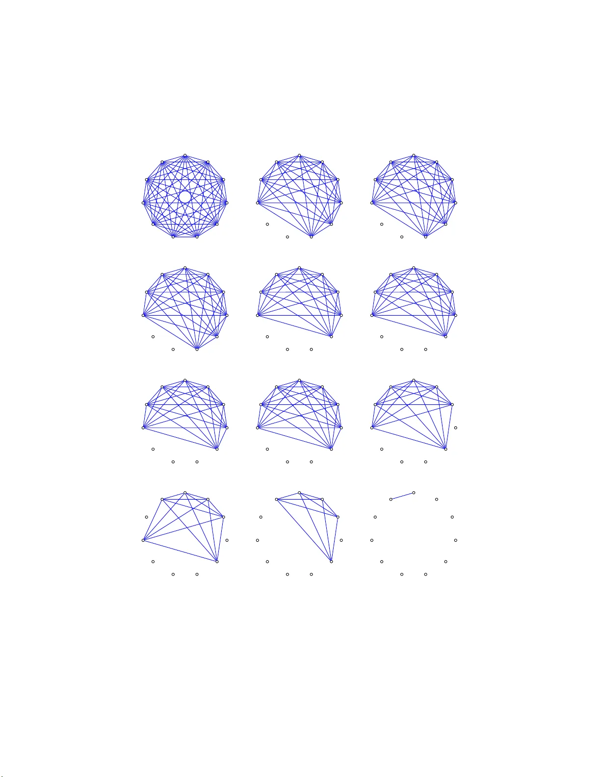
Sparse in v erse co v ariance estimation with the lasso Jer ome Friedman ∗ Trev or Hastie † and R ober t Tibshirani ‡ Octob er 23, 201 8 Abstract W e consid e r th e problem of estimating sparse graphs by a lasso p enalt y applied to the inv erse co v ariance matrix. Using a co ordinate descen t pro cedure for the lasso, we dev elop a simple algorithm that is remark ably fast: in the worst cases, it solv es a 1000 no de p roblem ( ∼ 500 , 000 parameters) in ab out a min ute, and is 50 to 2000 times faster than comp eting metho ds. It also p ro vides a conceptual link b et ween the exact problem and th e app ro ximation suggested by Meinshausen & B ¨ uhlmann (2006 ). W e illustrate th e metho d on some cell-signaling data fr o m proteomics. 1 In tro ducti on In recen t y ears a n umber of authors hav e prop osed the estimation of sparse undirected graphical mo dels through the use of L 1 (lasso) regularization. The basic mo del for con tin uous data assumes that the observ atio ns ha v e a m ultiv ariate Gaussian distribution with mean µ and co v ar ia nc e matrix Σ. If the ij th comp onen t of Σ − 1 is zero, then v ariables i and j are conditionally ∗ Dept. of Statistics , Stanford Univ., CA 94 305, jhf@stanford.edu † Depts. of Statistics, and Health, Research & Policy , Stanford Univ., CA 94 305, hastie@stanfor d.edu ‡ Depts. of Health, Rese arc h & Policy , and Statistics, Stanford Univ, tibs@sta n for d.edu 1 indep e nden t, giv en the other v ariables. Th us it mak es sense to imp ose a n L 1 p enalt y for t he estimation of Σ − 1 . Meinshausen & B¨ uhlmann ( 2 006) tak e a simple approac h to this problem: they estimate a sparse graphical mo del by fitting a lasso mo del to each v ari- able, using the others as predictors. The comp one nt ˆ Σ − 1 ij is then estimated to b e non-zero if either the estimated co effi cien t of v ariable i on j , or the estimated co efficien t of v ariable j on i , is non-zero (alternative ly they use an AND rule). They sho w that a symptotically , this consisten tly estimates the set of non-zero elemen ts of Σ − 1 . Other authors ha v e prop osed algorit h ms for the exact maximization of the L 1 -p enalized log -lik eliho o d; b oth Y uan & Lin (200 7) and Banerjee et al. (2007) adapt interior p o in t optimization metho ds for the solution to this problem. Both pap ers also establish that the simpler approac h of Mein- shausen & B ¨ uhlmann (2006) can b e view ed as an approximation to the exact problem. W e use the dev elopmen t in Banerjee et al. (2 007) as a launching p oin t, and prop ose a simple, lasso-style algorithm for the exact problem. This new pro cedure is extremely simple, and is substan tially faster than the in terior p oin t approac h in our tests. It also bridges the “conceptual gap” b et w een the Meinshausen & B ¨ uhlmann (2006) pro posal and the exact problem. 2 The prop o sed metho d Supp ose w e hav e N multiv ariate no r ma l observ ations of dimension p , with mean µ and cov ariance Σ. F ollo wing Banerjee et al. (200 7 ), let Θ = Σ − 1 , and let S b e the empirical cov ariance matrix, the pro blem is to maximize the log-lik eliho o d log det Θ − t r( S Θ) − ρ || Θ || 1 , (1) where tr denotes the trace and || Θ || 1 is the L 1 norm— the sum of the absolute v alues of the elemen ts of Σ − 1 . Expression (1 ) is the G aussian log- lik eliho o d of the data , partially maximized with resp ect to the mean para meter µ . Y uan & Lin (200 7) solve this problem using the interior p o in t metho d for the “maxdet” problem, prop o sed by V anden b erghe et al. (19 98). Banerjee et al. ( 2 007) dev elop a differen t framew ork f or the optimization, whic h w as the imp etus f or our w ork. 2 Banerjee et al. (2007 ) show that the problem ( 1) is conv ex and consider estimation of Σ (rather t han Σ − 1 ), as follo ws. Let W b e the estimate of Σ. They show that o ne can solv e the problem b y o ptimizing o v er each row and corresp onding column o f W in a blo ck co ordinate descen t fa shion. P artition- ing W and S W =  W 11 w 12 w T 12 w 22  , S =  S 11 s 12 s T 12 s 22  , (2) they sho w that the solutio n for w 12 satisfies ˆ w 12 = argmin y { y T W − 1 11 y : | | y − s 12 || ∞ ≤ ρ } . (3) This is a b o x-constrained quadrat ic prog r a m whic h they solv e using an in te- rior p oin t pro cedure. P erm uting the ro ws and columns so the target column is alw ays the last, they solv e a problem lik e (3) for each column, up dating their estimate o f W after each stage. This is rep eat ed until con v ergence. Us- ing con v ex dualit y , Ba nerjee et al. (2007) go on to sho w that (3) is equiv alen t to the dual problem min β || W 1 / 2 11 β − b || 2 + ρ || β | | 1 , ( 4 ) where b = W − 1 / 2 11 s 12 / 2. This expression is the basis f o r our approac h. First w e note that it is easy to ve rify the equiv alence betw een the solutions to (1) a nd (4) directly . The sub-gra dient equation for maximization of the log-lik eliho o d (1 ) is W − S − ρ · Γ = 0 , (5) using the fact that t he deriv ativ e of log det Θ equals Θ − 1 = W , g iv en in e.g Bo yd & V andenberghe (2004), page 641. Here Γ ij ∈ sign(Θ ij ); i.e. Γ ij = sign(Θ ij ) if Θ ij 6 = 0, else Γ ij ∈ [ − 1 , 1] if Θ ij = 0. No w the upp er right blo ck of equation (5) is w 12 − s 12 − ρ · γ 12 = 0 , (6) using the same sub-matrix no tation as in (2). On the other ha nd, the sub-gradient equation from (4) works out to b e 2 W 11 β − s 12 + ρ · ν = 0 , (7) where ν ∈ sign( β ) elemen t -wise. 3 No w suppo se ( W, Γ) solv es (5), and hence ( w 12 , γ 12 ) solve s (6). Then β = 1 2 W − 1 11 w 12 and ν = − γ 12 solv es (7). The equiv alence of the first t w o terms is ob vious. F or the sign terms, since W 11 θ 12 + w 12 θ 22 = 0, w e hav e that θ 12 = − θ 22 W − 1 11 w 12 (partitioned-inv erse form ula). Since θ 22 > 0, then sign( θ 12 ) = − sign( W − 1 11 w 12 ) = − sign( β ). No w to the main p oint of t his pap er. Problem (4) lo oks lik e a la sso ( L 1 - regularized) least squares problem. In fact if W 11 = S 11 , then the solutions ˆ β are easily seen to equal one-half of the lasso estimates f o r the p th v a riable on the others, and hence related to the Meinshausen & B ¨ uhlmann (2006) prop osal. As p o inted out by Banerjee et al. (2007), W 11 6 = S 11 in general and hence the Meinshause n & B ¨ uhlmann (20 06) approa c h do es not yield the maxim um like liho o d estimator. They point out that their blo c k-wise in terior-p oin t procedure is equiv alen t to recursiv ely solving a nd up da ting the lasso problem (4), but do not pursue this approac h. W e do, to great adv an tag e, b ecause fast co ordinate descen t algorithms (F riedman et al. 2007 ) mak e solution of the lasso problem v ery attractive . In terms of inner pro ducts, the usual lasso estimates for the p th v a riable on the ot hers take as input the data S 11 and s 12 . T o solv e (4) w e instead use W 11 and s 12 , where W 11 is our curren t estimate of the upp er blo c k o f W . W e then up date w and cycle throug h all of the v aria bles un til con v ergence. Note that from (5), the solution w ii = s ii + ρ for all i , since θ ii > 0, and hence Γ ii = 1. Here is our algorithm in detail: Covarianc e L asso Algorithm 1. Start with W = S + ρI . The diagonal of W remains unch anged in what follo ws. 2. F or eac h j = 1 , 2 , . . . p, 1 , 2 , . . . p, . . . , solve the lasso problem (4), whic h tak es as input the inner pro ducts W 11 and s 12 . This giv es a p − 1 v ector solution ˆ β . Fill in the corresp onding row a nd column of W using w = 2 W 11 ˆ β . 3. Con tinue un til con ve rgence Note again that eac h step in step (2) implies a p erm utation of the ro ws and columns to make the t a rget column the last. The lasso pro blem in step (2) ab o v e can b e efficien tly solv ed b y co ordinate descen t (F riedman et al. 4 (2007),W u & L a nge (2007)). Here a r e t he details. Letting V = W 11 , then the up date ha s the form ˆ β j ← S ( s 12 j − 2 X k 6 = j V k j ˆ β k , ρ ) / (2 V j j ) (8) for j = 1 , 2 , . . . p, j = 1 , 2 , . . . p, . . . , where S is the soft- threshold op erator: S ( x, t ) = sign( x )( | x | − t ) + . (9) W e cycle thro ug h the predictors until conv ergence. Note that ˆ β will t ypically b e sparse, and so the computatio n w = 2 W 11 ˆ β will b e fast: if there are r non-zero elemen ts, it ta kes r p op erations. Finally , supp ose our final estimate of Σ is ˆ Σ = W , and store the estimates ˆ β fro m the ab ov e in the rows and columns of a p × p matrix ˆ B (not e that the diagonal of ˆ B is not determined). Then w e can obta in the p th row (and column) of ˆ Θ = ˆ Σ − 1 = W − 1 as fo llows: ˆ Θ pp = 1 W pp − 2 P k 6 = p ˆ B k p W k p ˆ Θ k p = − 2 ˆ Θ pp ˆ B k p ; k 6 = p (10) In terestingly , if W = S , these are just the f o rm ulas for obtaining the inv erse of a part it io ned matrix. That is, if w e set W = S and ρ = 0 in the ab ov e algorithm, t hen one sw eep throug h the predictors computes S − 1 , usin g a linear regression at eac h stage. 3 Timing compariso ns W e sim ulated Gaussian data fro m b oth sp arse and dense scenarios, for a range o f problem sizes p . The sparse scenario is the AR(1) mo del tak en from Y uan & Lin (200 7): β ii = 1, β i,i − 1 = β i − 1 ,i = 0 . 5, and zero otherwise. In the dense scenario, β ii = 2, β ii ′ = 1 otherwise. W e c hose the t he penalty parameter so that the solution had ab o ut the actual n um b er of non-zero elemen ts in the sparse setting, a nd ab out ha lf of total n um b er of elemen ts in the dense setting. The conv ergence threshold w as 0 . 0001. The co v aria nce lasso pro cedure w as co ded in F ortran, linked to an R language function. All timings we re carried out on a In tel Xeon 2.80GH pro cessor. 5 p Problem (1) Co v aria nce (2) Approx (3) CO VSEL Ratio of T yp e Lasso (3) to (1) 100 sparse .018 .007 34.67 1926.1 100 dense .038 .018 2.17 57.1 200 sparse .070 .027 > 20 5 . 35 > 2933 . 6 200 dense .324 .146 16.87 52.1 400 sparse .601 .193 > 16 16 . 66 > 2690 . 0 400 dense 2.47 .752 313.04 126.5 T able 1: Tim ings (se c on ds) for c ovarianc e lasso, Meinhausen-Buhlmann a p- pr oximation, and COVSEL pr o c e dur es. W e compared the cov a riance lasso to the CO VSEL pr o gram pro vided by Banerjee et al. ( 2 007). This is a Matla b program, with a lo o p that calls a C language co de to do the b o x-constrained QP for eac h column of the solution matrix. T o b e as fa ir as p ossible to CO VSEL, we only coun ted the CPU time sp en t in the C program. W e set the maxim um n um b er of outer iterations to 30, and follow ing the authors co de, set the the duality g ap for con v ergence to 0.1. The n um b er of CPU seconds for eac h tria l is shown in T able 1. In t he dense scenarios for p = 200 and 4 0 0, CO VSEL had not con verged by 3 0 iterations. W e see that the cov ariance Lasso is 50 to 2000 times faster than CO VSEL, and only ab out 3 times slow er tha n the a pproximate metho d. Th us the co v ariance lasso is taking only ab out 3 passes through the the columns of W on a v erage. Figure 1 sho ws the num b er of CPU seconds required for the co v ariance lasso pro cedure, for problem sizes up to 1000. Ev en in the dense scenario, it solv es a 1 0 00 no de problem ( ∼ 500 , 000 parameters) is ab out a minu te. 4 Analysis of cell signalling data F or illustration w e analyze a flo w cytometry dataset on p = 11 pro teins and n = 7 466 cells, from Sac hs et al. (2 0 03). These authors fit a directed acyclic graph (DA G ) to the data, pro ducing the netw ork in Figure 2. The result of applying the co v ariance Lasso t o these data is show n in Figure 3, fo r 12 differen t v alues of the penalty parameter ρ . There is mo derate 6 200 400 600 800 1000 0 10 20 30 40 50 60 70 Number of variables p Number of seconds sparse dense Figure 1: N umb er of CPU se c onds r e quir e d for the c ovarianc e lasso pr o c e dur e. Raf Mek Plcg PIP2 PIP3 Erk Akt PKA PKC P38 Jnk Figure 2: D i r e cte d acylic gr aph fr om c el l-signaling data, fr om Sachs et al. (2003). 7 Raf Mek Plcg PIP2 PIP3 Erk Akt PKA PKC P38 Jnk L1 norm= 2.06117 Raf Mek Plcg PIP2 PIP3 Erk Akt PKA PKC P38 Jnk L1 norm= 0.09437 Raf Mek Plcg PIP2 PIP3 Erk Akt PKA PKC P38 Jnk L1 norm= 0.04336 Raf Mek Plcg PIP2 PIP3 Erk Akt PKA PKC P38 Jnk L1 norm= 0.02199 Raf Mek Plcg PIP2 PIP3 Erk Akt PKA PKC P38 Jnk L1 norm= 0.01622 Raf Mek Plcg PIP2 PIP3 Erk Akt PKA PKC P38 Jnk L1 norm= 0.01228 Raf Mek Plcg PIP2 PIP3 Erk Akt PKA PKC P38 Jnk L1 norm= 0.00927 Raf Mek Plcg PIP2 PIP3 Erk Akt PKA PKC P38 Jnk L1 norm= 0.00687 Raf Mek Plcg PIP2 PIP3 Erk Akt PKA PKC P38 Jnk L1 norm= 0.00496 Raf Mek Plcg PIP2 PIP3 Erk Akt PKA PKC P38 Jnk L1 norm= 0.00372 Raf Mek Plcg PIP2 PIP3 Erk Akt PKA PKC P38 Jnk L1 norm= 0.00297 Raf Mek Plcg PIP2 PIP3 Erk Akt PKA PKC P38 Jnk L1 norm= 7e−05 Figure 3: Cel l-signaling data: undir e cte d gr aphs fr om c ovarianc e lasso with dif- fer ent values of the p enalty p ar ameter ρ . 8 agreemen t b et w een, f o r example, the graph for L1 norm = 0 . 0 0496 and the D AG: the former ha s ab out half of the edges and non-edges that app ear in the DA G. Figure 4 show s the lasso co efficien ts as a function of tot a l L 1 norm of the co efficien t ve ctor. In the left panel of Figure 5 w e tried tw o differen t kinds of 10-fo ld cross- v alidation for estimation of the para meter ρ . In the “Regr ession” appro ac h, w e fit the co v ariance-lasso to nine-t en ths of the dat a , and used the p enalized regression mo del fo r each pro tein to predict the v alue o f that protein in the v alidation set. W e then av erag ed the squared prediction errors ov er all 11 proteins. In the “Lik eliho o d” approac h, w e again applied the cov ariance- lasso to nine-tenths of the data, and then ev aluat ed the lo g-lik eliho o d (1 ) o v er the v alidation set. The tw o cross-v alidation curv es indicate that the unregularized mo del is the b est, not surprisin g giv e the large n umber of observ ations and relative ly small num b er of parameters. Ho w ev er we also see that the lik eliho o d approach is far less v ariable than the regression metho d. The right panel compares the cross-v alidated sum o f squares of the exact co v ariance lasso approach to the Meinhausen-Buhlmann a ppro ximation. F or ligh tly regularized mo dels, the exact approach has a clear adv an tage. 5 Discuss ion W e ha v e presen ted a simple a nd fa st alg o rithm for estimation of a sparse in v erse co v aria nce matrix using a n L 1 p enalt y . It cycles throug h the v ariables, fitting a mo dified la sso regr ession to eac h v ariable in turn. The individual lasso problems are solved by co ordinate descen t . The sp eed of this new pro cedure s hould facilitate the application of sparse in v erse co v ariance pro cedures to large datasets inv olving thousands of param- eters. F or t r an and R la nguage routines fo r the prop osed metho ds will b e made freely av ailable. Ac knowle dgmen ts W e thank the authors of Ba nerjee et al. (200 7) for making t heir COVSEL program publicly a v ailable, and Larry W asserman for helpful discussions. F riedman was partially supp orted b y gran t D MS-97-64 431 from the National Science F oundation. Hastie was partially supp or t ed by gra nt DMS-0505 676 9 0.0 0.5 1.0 1.5 2.0 −0.6 −0.4 −0.2 0.0 L1 norm beta Raf−Mek Raf−Erk Raf−PKC Plcg−PIP2 Erk−Akt PKC−P38 PKC−Jnk Figure 4: Cel l-signaling data: pr ofile of c o efficients as the total L 1 norm of the c o- efficient ve ctor incr e ases, that is, as ρ de cr e ases. Pr ofiles for the lar gest c o effici e nts ar e lab ele d with the c orr esp onding p air of pr oteins. 10 1e−04 1e−02 1e+00 40 60 80 100 log L1 norm cv error Regression Likelihood 1e−04 1e−02 1e+00 100 200 300 400 log L1 norm cv error Exact Approximate Figure 5 : Cel l-signaling data. L eft p anel shows tenfold cr oss-validation u si ng b oth R e gr ession a nd Likeliho o d appr o aches (details in text). Right p anel c omp ar es the r e- gr ession sum of squar es of the exact c ovarianc e lasso appr o ach to the M einhausen- Buhlmann appr oximation. 11 from the National Science F oundation, and grant 2R01 CA 72028- 07 from the National Institutes of Health. Tibshirani w as part ia lly supp orted by National Science F oundation Gra n t DMS-99714 05 and National Institutes of Health Contract N01-HV-2 8 183. References Banerjee, O., Ghaoui, L. E. & d’Aspremon t, A. (2 007), ‘Mo del selection through sparse maxim um lik eliho o d estimation’, T o app e ar, J. Machine L e arn ing R ese ar ch 101 . Bo yd, S. & V anden b erghe, L. (2004), Convex Optimization , Cam bridge Uni- v ersit y Press. F riedman, J., Hastie, T. & Tibshirani, R. (2007 ), ‘P ath wise co ordina t e opti- mization’, Annals of Applie d Statistics, to app e ar . Meinshausen, N. & B ¨ uhlmann, P . (2 0 06), ‘High dimensional graphs and v ari- able selection with the lasso’, Annals o f Statistics 34 , 1 436–146 2 . Sac hs, K., Pe rez, O., P e’er, D ., Lauffen burger, D. & Nolan, G. ( 2 003), ‘Causal protein-signaling net w orks deriv ed from m ultiparameter single- cell data’, Scienc e (308 (5721)), 50 4–6. V anden b erghe, L., Bo yd, S. & W u, S.-P . (1998), ‘Determinan t maximiza- tion with linear matrix inequalit y constrain ts’, SIAM Journal o n Matrix A nalysis and Applic ations 19 (2), 4 99–533. *citeseer.ist.ps u.edu/v andenberghe98determinan t.html W u, T. & Lange, K. (2007), Co or dina t e descen t pro cedures for lasso penalized regression. Y uan, M. & Lin, Y. (2007) , ‘Mo del selection a nd estimation in the gaussian graphical mo del’, Biometrika 94 (1), 19–35. 12