Dynamic Modeling and Statistical Analysis of Event Times

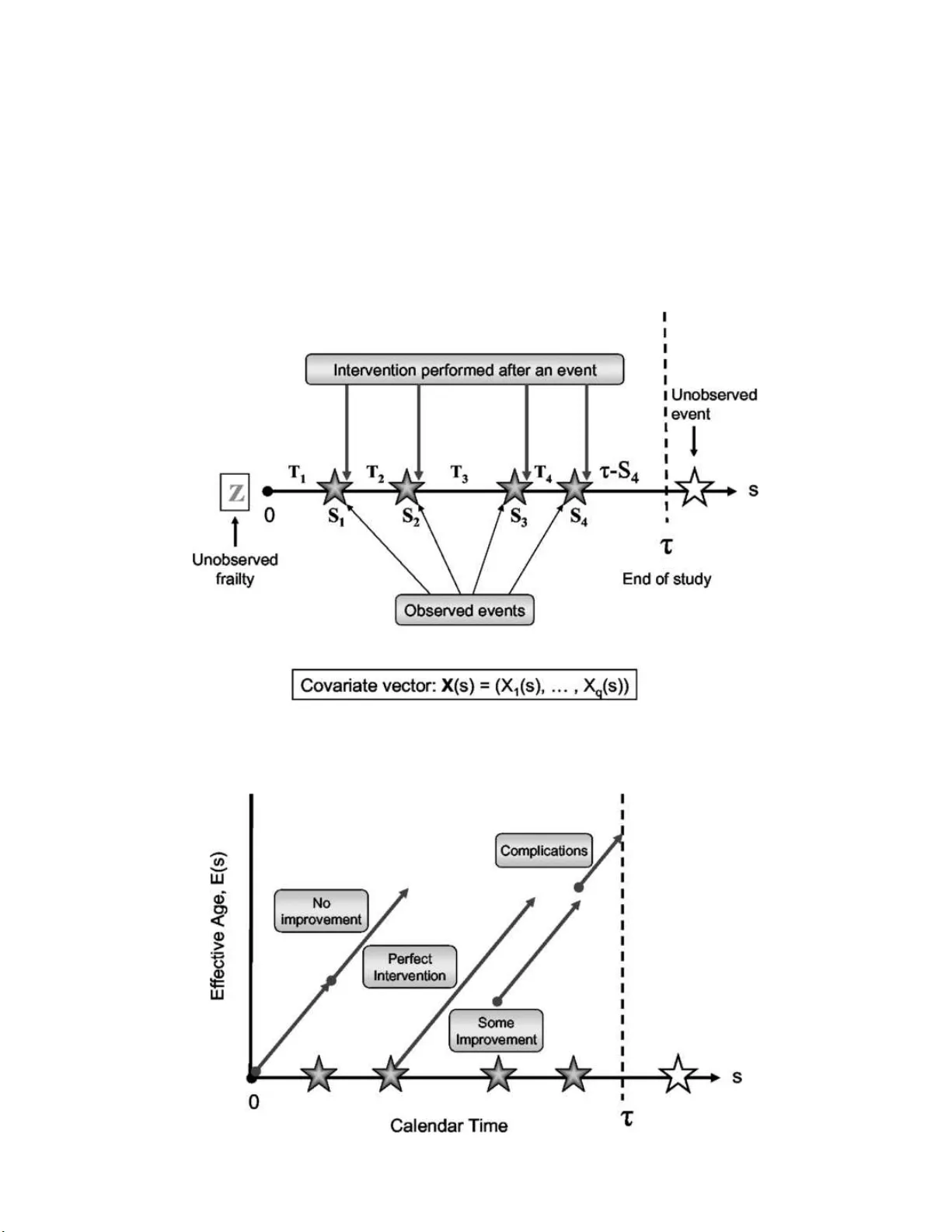
Statistic al Scienc e 2006, V ol. 21 , N o. 4, 487– 500 DOI: 10.1214 /0883423 06000000349 c  Institute of Mathematical Statistics , 2006 Dynamic Mo deling and Statistical Analysis of Event Times Edsel A. P e˜ na Abstr act. This review article provi des an o ve rview of recen t work in the mo deling and analysis of recurrent ev en ts arising in engineering, reliabilit y , public healt h, b iomedicine and o ther areas. Recurren t ev en t mo deling p o ssesses unique facets m aking it differen t and m ore diffi- cult to handle than sin gle ev ent settings. F or instance, the imp act of an increasing n umber of ev en t o ccurrences needs to b e tak en in to ac- coun t, the effects of co v ariate s sh ould b e considered, p otent ial asso- ciatio n among the in terev en t times within a u nit cannot b e ignored, and the effects of p erformed in terv en tions after eac h even t o ccurrence need to b e factored in. A recen t general class of mo d els for recurr en t ev en ts wh ic h simult aneously a ccommo dates these aspects is describ ed. Statistica l inference metho ds for this cl ass of m o dels are presen ted and illustrated through applications to r eal data s ets. Some existing op en researc h problems are described . Key wor ds and phr as es: Coun ting p ro cess, hazard function, martin- gale, p artial lik elihoo d, generalized Nelson–Aale n estimator, general- ized p ro duct-limit estimator. 1. INTRODUCTION A decade ago in a Statistic al Scienc e article, Singpurwalla ( 1995 ) adv ocated the deve lopment, adoption and exploration of dynamic mo dels in the theory and practice of rel iabilit y . He also pinp oin ted that the u se of sto c hastic pr o cesses in the mo del- ing of comp onen t and system failure times offers a ric h envi ronment to meaningfully capture dynamic op erating conditions. In this article, we review r e- cen t researc h d ev elopmen ts in d ynamic fai lure-time mo dels, in the con text of b oth stochasti c mo del- ing and i nference concerning mo del parameters. Dy- namic mo dels are not limited in app licabilit y and relev ance to the engineering and relia bilit y areas. Edsel A. Pe˜ na is Pr ofessor, Dep artment of Statistics, University of South Car oli na, Columbia, South Car olina 29208 , USA e-mail: p ena@stat.sc.e du . This is an electronic reprint o f the original article published b y the Institute of Mathematical Statistics in Statistic al Scienc e , 200 6, V ol. 21, No. 4, 487 –500 . This reprint differs from the orig inal in pagination and t yp ogr aphic detail. They are also relev an t in other fields such as pu blic health, biomedicine, economics, so ciology and p oli- tics. This is b ec ause in man y studies in these v ar- ied a reas, it is often times of int erest to monitor the o ccurrences of an ev en t. Suc h an ev en t could b e the malfunctioning of a mec hanical or electronic system, encoun tering a b ug in computer soft wa re, the out- break of a disease, o ccurren ce of a migraine, reo c- currence of a tumor, a d rop of 200 p oin ts in the Do w Jones Ind ustrial Av erage du ring a trading d a y , com- mission of a criminal ac t in a cit y , serious disagree- men ts b et ween a married couple, or the replacemen t of a cabinet min ister/secreta ry in an administration. These ev en ts recur and s o it is of inte rest to de- scrib e their recurrence b eha vior through a sto c hastic mo del. I f suc h a mo del has excellen t predictiv e abil- it y for ev en t occurrences, then if ev ent o ccurrences lead to drastic and/or negativ e consequences, pre- v en tiv e inte rven tions may b e attempted to minimize damages, whereas if they lead to b eneficial and/or p ositiv e outcomes, certain actions may b e p erform ed to hasten ev en t occurrences. It is b ecause of p erformed in terv en tions after ev en t o ccurrences that dynamic mo dels b e come especially 1 2 E. A. PE ˜ NA p ertinent , sin ce through su c h inte rven tions, or some- times nonin terve nti ons, the sto chastic structure go v- erning future ev en t o ccurr ences is altered. This c hange in the mec hanism go v erning the even t o ccurr ences could also b e due to the induced c hange in the struc- ture f unction in a reliabilit y setting go v erning the system of in terest arising from an ev en t o ccurrence (cf. Hollander and P e ˜ na, 1995 ; Kv am and P e ˜ na, 2005 ; P e ˜ na and Slate, 2005 ). F urthermore, since sev eral ev en ts may occur within a un it, it is also imp ortan t to consider the asso ciation among the in terev en t times whic h ma y arise b ecause of unobserv ed ran- dom effects or frailties for the u nit. In addition, there is a need to tak e in to accoun t the p oten tial impact of environmen tal and other relev ant co v ari- ates, p o ssibly includ in g the accumulat ed n umber of ev en t o ccurrences, which could affect future even t o ccurrences. In this review article w e describ e a flexible and general class of dynamic sto c hastic mo dels for even t o ccurrences. This class of mod els wa s prop osed by P e ˜ na and Hollander ( 2004 ). W e also discuss infer- ence metho d s for this class of mo d els as deve lop ed in P e˜ n a, Str awderman and Hollander ( 2001 ), Pe˜ na, Slate and Gonz´ alez ( 2007 ) and Kv am and P e˜ na ( 2005 ). W e demonstrate their app licatio ns to real data s ets and ind icate some open researc h p roblems. 2. BA CK GROUND AND NOT A TION Rapid and general progress in eve nt time mo d- eling and inference has b enefited immensely from the adoption of the framewo rk of count ing pro cesses, martingales and sto c hastic integ ration as in tro du ced in Aalen’s ( 1978 ) pioneering work. The presen t re- view article adopts this mathematica l framewo rk. Excellen t references for this framewo rk are the mono- graph of Gill ( 1980 ), and the b o oks b y Fleming and Harrington ( 1991 ) and Andersen , Borgan, Gill and Keiding ( 1993 ). W e introd uce in this section some notation and v ery minimal bac kground in order to help the reader in the sequel, b u t advise the reader to consult the aforement ioned references to gain an in-depth knowle dge of this framew ork. W e denote b y (Ω , F , P ) the basic probabilit y space on wh ich all rand om en tities are defined . Since in - terest will b e on times b et we en ev ent o ccurrences or on the times of eve nt o ccurr ences, nonn egativ e- v al ued random v aria bles will b e of concern. F or a random v ariable T with range ℜ + = [0 , ∞ ), F ( t ) = F T ( t ) = P { T ≤ t } and S ( t ) = S T ( t ) = 1 − F ( t ) = P { T > t } will d enote its distribution and survivo r (also calle d reliabilit y) f u nctions, r esp ectiv ely . The indicator fun ction of the even t A will b e denoted b y I { A } . The cumula tiv e hazard function of T is defined according to Λ( t ) = Λ T ( t ) = I { t ≥ 0 } Z t 0 F ( d w ) S ( w − ) with the co nv en tion that S ( w − ) = lim t ↑ w S ( t ) = P { T ≥ w } and R b a · · · = R ( a,b ] · · · . F or a nondecreasing function G : ℜ + → ℜ + with G (0) = 0, its pro d uct- in tegral o v er (0 , t ] is defined via (cf. Gill and Jo- hansen, 1990 ; Andersen et al., 1993 ) Q t w =0 [1 − G ( dw )] = lim M →∞ Q M i =1 [1 − ( G ( t i ) − G ( t i − 1 ))], where as M → ∞ , the partition 0 = t 0 < t 1 < · · · < t M = t 0 satisfies max 1 ≤ i ≤ M | t i − t i − 1 | → 0. The survivo r fun c- tion in te rms o f the cumulat ive hazard fun ction b e- comes S ( t ) = I { t < 0 } + I { t ≥ 0 } t Y w =0 [1 − Λ( dw )] . (2.1) F or a discrete random v ariable T with j ump p o ints { t j } , the h azard λ j at t j is the conditional p robabil- it y that T = t j , giv en T ≥ t j , so Λ( t ) = P { j : t j ≤ t } λ j . If T is an absolutely con tin uous random v ariable with densit y fun ction f ( t ), its hazard rate function is λ ( t ) = f ( t ) /S ( t ) , so Λ( t ) = R t 0 λ ( w ) dw = − log S ( t ). The p ro duct-in tegral r epresen tation of S ( t ) ac cord- ing to wh ether T is purely discrete or p urely con tin- uous is S ( t ) = t Y w =0 [1 − Λ( dw )] (2.2) =        Y t j ≤ t [1 − λ j ] , if T is discrete, exp  − Z t 0 λ ( w ) dw  , if T is con tin uous. A b enefit of using hazards or h azard rate functions in mo deling is that they provide qu alitati ve asp e cts of the ev ent o ccurr ence pro cess as time progresses. F or instance, if the hazard rate fu n ction is increas- ing (decreasing) then this indicate s that the ev en t o ccurrences are in creasing (decreasing) as time in- creases, and thus we ha ve th e n otion of increasing (decreasing) failure rate [IFR (DFR)] distribu tions. F or man y y ears, it was the fo cus of theoretical re- liabilit y researc h to deal with cl asses of distribu - tions suc h as IFR, DFR, increasing (decreasing) fail- ure rate on a v erage [IFRA (DFRA)], and so on, MODELING AND ANAL YSIS OF EVENT TIMES 3 sp ecifically with regard to their closure prop erties under certain reliabilit y op erations (cf. Barlo w and Prosc han, 1981 ). In monito ring an exp e rimenta l unit for the o c- currence of a recurrent ev ent , it is con v enien t and adv an tag eous to utilize a coun ting p ro cess { N ( s ) , s ≥ 0 } , wh ere N ( s ) denotes the num b er of times that the ev ent has o ccurred ov er the interv al [0 , s ]. The paths of this sto c hastic pro cess are step-fu n ctions with N (0) = 0 and with ju mps of un it y . If w e rep- resen t the calendar times of ev en t o ccurr ences b y S 1 < S 2 < S 3 < · · · with the con v en tion that S 0 = 0, then N ( s ) = P ∞ j =1 I { S j ≤ s } . Th e interev ent times are denoted b y T j = S j − S j − 1 , j = 1 , 2 , . . . . In sp e ci- fying the sto c hastic c haracteristic s of the ev en t o ccurrence pro c ess, one either sp eci fies all the finite- dimensional distributions of the pro cess { N ( s ) } , or sp ecifies the join t d istributions of the S j ’s or the T j ’s. F or example, a common sp ecification for even t o ccurrences is the assumption of a homogeneous P ois- son pro cess (HPP) w here the in terev en t times T j are indep end en t and iden tically distributed exp o nentia l random v aria bles w ith scale β . This is equiv alen t to s p ecifying th at, for any s 1 < s 2 < · · · < s K , the random v ectors ( N ( s 1 ) , N ( s 2 ) − N ( s 1 ) , . . . , N ( s K ) − N ( s K − 1 )) hav e indep endent comp onent s with N ( s j ) − N ( s j − 1 ) ha ving a Poisson d istribution with param- eter β ( s j − s j − 1 ). F rom this sp ec ification, the finite- dimensional distributions of ( N ( s 1 ) , N ( s 2 ) , . . . , N ( s K )) ca n b e obtained. An imp ortan t concept in dynamic mo deling is that of a history or a fi ltration, a family of σ -fields F = {F s : s ≥ 0 } w here F s is a sub- σ -field of F with F s 1 ⊆ F s 2 for ev ery s 1 < s 2 and with F s = T h ↓ 0 F s + h , a righ t-con tin uit y prop erty . On e int erprets F s as all information that accrued o v er [0 , s ]. When augmen ted in (Ω , F , P ), we obtain the fi ltered pr obabilit y space (Ω , F , F , P ). It is with resp ec t to suc h a filtered probabilit y space that a pr o cess { X ( s ) : s ≥ 0 } is said to b e adapted [ X ( s ) is measurable with resp ect to F s , ∀ s ≥ 0]; is said to b e a (sub)martingale [adapted, E | X ( s ) | < ∞ , and , ∀ s, t ≥ 0, E { X ( s + t ) |F s } ( ≥ ) = X ( s ) almost surely]. Do ob–Mey er’s decomp osition guaran tees that f or a submartingale Y = { Y ( s ) : s ≥ 0 } there is a unique increasing pr ed ictable (measur- able with resp ect to the σ -field generated by adapted pro cesses with left-c ont inuous paths) pro cess A = { A ( s ) : s ≥ 0 } , called the comp ensator, with A (0) = 0 suc h that M = { M ( s ) = Y ( s ) − A ( s ) : s ≥ 0 } is a martingale. Via Jensen’s inequalit y , then for a square-in tegrable martingale X = { X ( s ) : s ≥ 0 } , there is a unique comp ensator pro cess A = { A ( s ) : s ≥ 0 } su c h that X 2 − A is a martingale. Th is pro cess A , denoted b y h X i = {h X i ( s ) : s ≥ 0 } , is calle d the pre- dictable quadratic v ariation (PQV) pro cess of X . A useful heuristic, though somewhat impr ecise, wa y of presen ting the main prop erti es of martingales and PQV’s is through the follo wing different ial forms. F or a martingale M , E { dM ( s ) |F s − } = 0 , ∀ s ≥ 0; whereas for the PQV h M i , E { d M 2 ( s ) |F s − } = V ar { dM ( s ) |F s − } = d h M i ( s ) , ∀ s ≥ 0 . F or the HPP N = { N ( s ) : s ≥ 0 } w ith rate β and with F = {F s = σ { N ( w ) , w ≤ s } : s ≥ 0 } , N is a sub- martingale since its paths are n ondecreasing. Its com- p ensator pro cess is A = { A ( s ) = β s : s ≥ 0 } , so that M = { M ( s ) = N ( s ) − β s : s ≥ 0 } is a martingale. F urth erm ore, since N ( s ) is P oisson-distributed with rate β s , so that { M 2 ( s ) − A ( s ) = ( N ( s ) − β s ) 2 − β s : s ≥ 0 } is a martingale, the PQV pro cess of M is also A . T hrough the heur istic forms , w e h av e E { d N ( s ) |F s − } = dA ( s ) , s ≥ 0. Since dN ( s ) ∈ { 0 , 1 } , then w e obtain the probabilistic expression P { dN ( s ) = 1 |F s − } = dA ( s ) , s ≥ 0. Analogously , V ar { dN ( s ) | F s − } = E { [ dN ( s ) − dA ( s )] 2 |F s − } = dA ( s ) , s ≥ 0. These formula s hold for a general counti ng pr o cess { N ( s ) : s ≥ 0 } with compens ator pro cess { A ( s ) : s ≥ 0 } . In essence, cond itionally on F s − , dN ( s ) has a Bernoulli distribution with success probabilit y dA ( s ). Ov er the interv al [0 , s ], follo wing Jacod , the lik e- liho o d fun ction can b e written in pro duct-int egral form as L ( s ) = s Y w =0 { dA ( w ) } dN ( w ) { 1 − dA ( w ) } 1 − dN ( w ) (2.3) = ( s Y w =0 [ dA ( w )] dN ( w ) ) exp {− A ( s ) } , with the last equalit y holding when A ( · ) h as con tin- uous paths. Sto c hastic inte grals play a cru cial role in this stochas- tic pro cess framew ork for ev en t time mod eling. F or a square-in tegrable martingale X = { X ( s ) : s ≥ 0 } with PQV pro c ess h X i = {h X i ( s ) : s ≥ 0 } , and for a b ounded predictable pr o cess Y = { Y ( s ) : s ≥ 0 } , the sto c hastic in tegral of Y wit h resp e ct to X , de- noted by R Y dX = { R s 0 Y ( w ) dX ( w ) : s ≥ 0 } , is wel l defined. It is also a square-in tegrable martingale with PQV pro cess h R Y dX i = { R s 0 Y 2 ( w ) d h X i ( w ) : s ≥ 0 } . When X is asso ciated with a coun ting pro cess N , that is, X = N − A , the paths of the sto chasti c in- tegral R Y dX can b e tak en as path wise L eb esgue– Stieltjes inte grals. 4 E. A. PE ˜ NA Martingale theory also pla ys a ma jor role in ob- taining asymp totic pr op erties of estimators as fir st demonstrated in Aalen ( 1978 ), Gill ( 1980 ) and An - dersen and Gill ( 1982 ). The main to ols used in asymp- totic analysis are Lenglart’s inequalit y (cf. Lenglart, 1977 ; Fleming and Harrington, 1991 ; And ersen et al., 1993 ) whic h is used in p ro ving consistency , and Reb olledo’s ( 1980 ) martingale central limit theorem (MCL T) (cf. Fleming and Harrington, 1991 ; Ander- sen et al., 1993 ) whic h is used f or obtaining weak con v ergence resu lts. W e refer the reader to Fl eming and Harrington ( 1991 ) and Andersen et al. ( 1993 ) for the in-depth theory and applications of these mo dern to ols in failure-time analysis. 3. CLASS OF D YNAMIC MODELS Let us n o w consider a unit b e ing monitored o v er time for th e o ccurrence of a recurrent ev en t. T he monitoring p erio d could b e a fi xed in terv al or it could b e a random in terv al, and for our purp oses w e denote this p erio d by [0 , τ ] , where τ is assumed to h av e some distribu tion G , which ma y b e degen- erate. With a slight notat ional c hange from Sec- tion 2 we denote by N † ( s ) the n um b er of ev en ts that h a v e o ccurr ed on or b efore time s , and b y Y † ( s ) an indicator pro cess wh ic h equals 1 w h en the unit is still under observ ation at time s , 0 otherwise. With S 0 = 0 and S j , j = 1 , 2 , . . . , denoting the su c- cessiv e calendar times of eve nt o ccurrences, and with T j = S j − S j − 1 , j = 1 , 2 , . . . , b e ing the in terev en t or gap times, observ e th at N † ( s ) = ∞ X j =1 I { S j ≤ m in( s, τ ) } and (3.4) Y † ( s ) = I { τ ≥ s } . Asso ciated with the unit is a, p ossibly time-dep en- den t, 1 × q co v ariate v ector X = { X ( s ) : s ≥ 0 } . In re- liabilit y engineering stud ies, the comp onen ts of this co v ariate vect or could b e related to environmen tal or op erat ing condition charact eristics; in biomedical studies, they could b e blo o d pr essure, treatmen t as- signed, initial tumor size, and so on; in a so ciologic al study of marital d isharmon y , they could b e length of marr iage, family income lev el, n um b e r of children residing with the couple, ages of children, and so on. Usually , after eac h ev ent o ccurrence, some form of in terv en tion is applied or p erformed, such as replac- ing or repairing failed comp onent s in a r eliabilit y system, or reducing or increasing physical activit y after a heart attac k in a medical setting. These in ter- v en tions will t ypically imp act the next o ccurr ence of the ev en t. Th ere is fur th ermore recognition that for the unit the inte reve nt times are asso ciated or cor- related, p ossibly b ecause of unobserved random ef- fects or so-ca lled frailties. A pictorial r epresen tation of these asp ec ts is giv en in Figure 1 . Ob serv e that b ecause of the finiteness of th e monitoring p erio d, whic h leads to a su m-quota acc ru al sc heme, there will alwa ys be a right- censored in terev en t time. The observ ed num b er of ev en t occur r ences o v er [0 , τ ], K = N † ( τ ), is also informativ e ab out the sto chas- tic mec hanism go v erning ev en t o ccurrences. In fact, since K = max { k : P k j =1 T j ≤ τ } , then, conditionally on ( K, τ ), the v ector ( T 1 , T 2 , . . . , T K ) has d ep endent comp onen ts, ev en if at the outset T 1 , T 2 , . . . are in- dep endent. Recognizing these different asp ects in recurrent ev en t settings, P e ˜ na and Hollander ( 2004 ) prop osed a general class of mo dels that sim ultaneously incor- p orates all of these asp ects. T o describ e this class of mo d els, w e sup p ose that there is a filtration F = {F s : s ≥ 0 } su ch that for eac h s ≥ 0, σ { ( N † ( v ) , Y † ( v +) , X ( v + ) , E ( v +)) : v ≤ s } ⊆ F s . W e also assume that there exists an unobserv able p ositiv e r and om v aria ble Z , called a frailt y , whic h induces the cor- relation among the in ter-ev en t times. The class of mo dels of Pe˜ na and Hollander ( 2004 ) can now b e describ ed in differen tial f orm via P { dN ( s ) = 1 |F s − , Z } = Z Y † ( s ) λ 0 [ E ( s )] (3.5) · ρ [ N † ( s − ); α ] ψ ( X ( s ) β ) ds, where λ 0 ( · ) is a baseline hazard rate fu n ction; ρ ( · ; · ) is a nonnegativ e function with ρ (0; · ) = 1 and with α b eing some parameter; ψ ( · ) is a nonnegativ e link function with β a q × 1 regression p arameter v ector; and Z is a frailt y v ariable. The at-risk pr o cess Y † ( s ) indicates that the conditional probabilit y of an ev ent o ccurring b ec omes zero wheneve r the unit is not un- der observ ati on. Possible c hoices of the ρ ( · ; · ) and ψ ( · ) fun ctions are ρ ( k ; α ) = α k and ψ ( w ) = exp( w ), resp ectiv ely . F or the geo metric c hoice of ρ ( · ; · ), if α > 1 the effect of accumula ting ev en t o ccurrences is to accelerate ev ent o ccurrences, w hereas if α < 1 the ev en t o c curren ces d ecelerat e, the latter situa- tion appropriate in soft w are debu gging. T h e p ro cess E ( · ) app earing as argum ent in the baseline hazard rate function, called the effectiv e age p ro cess, is pre- dictable, observ able, nonn egativ e and pathwise al- most surely d ifferentia ble with deriv ativ e E ′ ( · ). Th is MODELING AND ANAL YSIS OF EVENT TIMES 5 effectiv e age pro cess m o dels th e impact of p erformed in terv en tions after eac h ev en t o ccurrence. A picto- rial depiction of this effect ive age pro cess is in Fig- ure 2 . In th is plot, after the first ev ent , the p e r- formed in terv ent ion has the effect of rev erting the unit to an effectiv e age equal to the age ju st b e- fore the ev ent o ccurrence (called a minimal repair or interv en tion), while after the second eve nt, th e p erformed inte rven tion h as the effect of rev erting the effecti ve age to that of a new unit (hen ce this is ca lled a p erfect in terv en tion or repair). After the third even t, the in terv ent ion is neither m in imal n or Fig. 1. Pictorial depiction of the r e curr ent event data ac crual for a unit il l ustr ating the window of observat ion [0 , τ ] , inter- vention p erforme d after an event o c curr enc e, an unobserve d fr ailty Z , the pr esenc e of a ve ctor of c ovar iates X , the inter event times T j and the c alendar times of event o c curr enc es S j . Fig. 2. An example of an effe ctive age pr o c ess, E ( s ) , for a unit enc ountering suc c essive o c curr enc es of a r e curr ent event. 6 E. A. PE ˜ NA p erfect and it has the effect of restarting the effectiv e age at a v alue b et wee n zero and that ju st b e fore the ev en t occurred; while for the four th ev en t, the inter- v en tion is detrimenta l in that the restarting effectiv e age exceeds that just b efore the even t o c curred . The effect iv e age pro c ess could o ccur in man y forms, and the idea is this sh ould b e determined in a dynamic fashion in conjunction with interv en- tions that are p erformed. As suc h the determination of this pro cess should preferably b e through con- sultations with exp erts of the sub ject matter u nder consideration. Common forms of this effecti ve age pro cess are: Minimal Interv en tion or Repair: (3.6) E ( s ) = s, P erfect Interv en tion or Repair: (3.7) E ( s ) = s − S N † ( s − ) , BBS Mo del: (3.8) E ( s ) = s − S Γ η ( s − ) , where in ( 3.8 ) with I 1 , I 2 , . . . b eing indep enden t Bernoulli random v ariables with I k ha ving success probabilit y p ( S k ) with p : ℜ + → [0 , 1], w e defi n e η ( s ) = P N † ( s ) i =1 I i and Γ 0 = 0, Γ k = min { j > Γ k − 1 : I j = 1 } , k = 1 , 2 , . . . . Thus, in ( 3.8 ), E ( s ) represen ts the time measured from s since the last p erfect re- pair. T h is effectiv e age is from Blo ck, Borge s and Sa vits ( 1985 ), w hereas when p ( s ) = p for some p ∈ [0 , 1], w e obtain the effectiv e age pro cess for the Bro wn and Prosc han ( 1983 ) minimal repair mo del. Clearly , the effectiv e age functions ( 3.6 ) and ( 3.7 ) are sp ecial cases of ( 3.8 ). Other effect iv e age pro- cesses that could b e u tilized are those associated with the general repair mo del of Kijima ( 1989 ), Stadje and Zuc ke rman ( 1991 ), Baxter, Kijima and T ortorella ( 1996 ), Dorado, Hollander and Sethuraman ( 1997 ) and Last and Szekli ( 1998 ). See also Lindqvist ( 199 9 ) and Lindqvist, Elve bakk and Heggland ( 2003 ) for a review of some of th ese mo del s p ertaining to re- pairable systems, and Gonz´ alez, Pe˜ na and Slate ( 2005 ) for an effe ctiv e age pro cess suitable f or cancer stud- ies. A cru cial prop e rty arising fr om the inte nsity sp ec - ification in ( 3.5 ) is it amounts to p ostulating that, with A † ( s ; Z, λ 0 ( · ) , α, β ) = Z Z s 0 Y † ( w ) λ 0 [ E ( w )] (3.9) · ρ [ N † ( w − ); α ] ψ ( X ( w ) β ) dw, then, conditionally on Z , the p ro cess { M † ( s ; Z, λ 0 ( · ) , α, β ) (3.10) = N † ( s ) − A † ( s ; Z, λ 0 ( · ) , α, β ) : s ≥ 0 } is a square-in tegrable martingale with PQV p ro cess A † ( · ; Z, λ 0 ( · ) , α, β ). The class of mo dels is general and flexible and su bsumes man y curren t mo dels for recurrent ev en ts utilized in surviv al analysis and reli- abilit y . In p articular, it includ es those of Jelinski and Moranda ( 1972 ), Gail, San tner and Bro wn ( 198 0 ), Gill ( 1981 ), Pr entice , Williams and P eterson ( 1981 ), La wless ( 1987 ), Aalen and Hus eb y e ( 1991 ), W ang and Chang ( 1999 ), Pe˜ na, Strawderman and Hollan- der ( 2001 ) a nd Kv am and P e ˜ na ( 200 5 ). W e demon- strate the class of mo d els via some concrete exam- ples. Example 1. The fi rst exa mple concerns a load- sharing K -comp onent parallel system with ident i- cal comp o nents. The recurr en t ev ent of in terest is comp onen t f ailure and f ailed comp onen ts are not re- placed. When a comp o nent fails, a redistribution of the system load o ccurs among the remaining fun c- tioning comp onents, and to mo del this system in a general w a y , we let α 0 = 1 and α 1 , . . . , α K − 1 b e p ositiv e co nstants, referred to as load-share param- eters. One p ossible sp ecificatio n of these p arameters is α k = K / ( K − k ) , k = 0 , 1 , 2 , . . . , K − 1, though they could b e un k n o wn constan ts, p ossibly ord ered. The hazard rate of ev en t o ccurrence at cale ndar time s , pro vided that the system is still under observ ation, is λ ( s ) = λ 0 ( s )[ K − N † ( s − )] α N † ( s − ) , where λ 0 ( · ) is the common h azard rate function of eac h comp o- nen t and N † ( s ) is the n umb er of comp onent fail- ures observ ed on or b efore ti me s . This is a sp ecial case of the general class of mo dels with E ( s ) = s , ρ ( k ; α 1 , . . . , α K − 1 ) = [ K − k ] α k , and ψ ( w ) = 1 . This is the equal load-sharing mo d el in Kv am and P e ˜ na ( 2005 ). More generally , this could accommo date en- vironmen tal or op erating condition co v ariates for the system, and even an unobserv ed frailt y comp o- nen t. Example 2. Assume in a soft w are reliabilit y m o del that there are α bugs at the b eginning of a debug- ging pro cess and the ev en t of inte rest is encoun ter- ing a bug. A p ossible mo del is these α bugs are MODELING AND ANAL YSIS OF EVENT TIMES 7 comp eting to b e encoun tered, and if eac h of them has h azard rate of λ 0 ( s ) o f b eing encounte red at time s , then the total hazard rate at time s of the soft w are failing is λ 0 ( s ) α . Up on encoun tering a bug at time S 1 , this bug is eliminated, th us d ecreasing the num b er of remaining bu gs b y one. T he debu g- ging p ro cess is then restarted at time jus t after S 1 (assuming it tak es zero time to eliminat e the bug, clearly a n o v ersimplification). In general, supp ose that just b efore calendar time s , N † ( s − ) bugs ha v e b een remo v ed, and the la st bug w as encountered at calendar time S N † ( s − ) . Then, the o ve rall h azard of encount ering a b ug at calendar time s with s > S N † ( s − ) is λ 0 ( s − S N † ( s − ) )[ α − N † ( s − )]. T h us, pro- vided that the debugging pro cess is still in progress at time s , then the hazard of en countering a bug at time s is λ ( s ) = λ 0 ( s − S N † ( s − ) ) max[0 , α − N † ( s − )]. Again, this is a sp ecial case of the general class of mo dels with E ( s ) = s − S N † ( s − ) , a consequence of the r estart of the debu gging pro cess, ρ ( k ; α ) = max { 0 , α − k } and ψ ( w ) = 1. This soft ware debug- ging mo del is th e mo del of Jelinski and Moranda ( 1972 ) and it w as also p rop osed by Gail, San tner and Bro wn ( 1980 ) as a carcinogenesis mo del. See also Agustin and P e˜ n a ( 1999 ) for another m o del in soft w are d ebugging wh ic h is a sp ecial case of the general class of mo dels. Co x’s ( 1972 ) p r op ortional hazards mo del is one of the most used mo d els in biomedical and p u blic health settings. Extensions of this mo del ha v e b een used in recurrent ev en t settings, and Th ern eau and Gram bsc h ( 2000 ) discuss some of these Co x-based mo dels suc h as the indep enden t incremen ts mo del of Andersen and Gill ( 1 982 ), the conditional mo del of Prentic e, Willi ams and Pete rson ( 1981 ) and the marginal mod el of W ei, Lin and W eissfeld ( 1989 ). The indep endent incremen ts mo d el is a sp ecial case of the general class of mo d els obtained b y ta king ei- ther E ( s ) = s or E ( s ) = s − S N † ( s − ) with ρ ( k ; α ) = 1 and ψ ( w ) = exp( w ) . The marginal mod el strati- fies according to the ev en t num b er and assumes a Co x-t yp e mo del for eac h of these strata, with the j th int erev ent time in the i th unit h a ving in tensit y Y ij ( t ) λ 0 j ( t ) exp { X i ( t ) β j } , where Y ij ( t ) equals 1 un- til the o ccurr ence of the j th even t or wh en the unit is ce nsored. The conditional mo del is similar to the marginal mo del except that Y ij ( t ) b ecomes 1 only after the ( j − 1)st ev en t h as o ccurred. 4. ST A TIS TICAL INFERENCE The relev ant parameters for the mo del in ( 3.5 ) are λ 0 ( · ), α , β and the parameter associated with the distribution of the fr ailt y v ariable Z . A v ariet y of forms for this frailt y distribu tion is p ossible, but w e restrict to the case where Z has a gamma distribu- tion with mean 1 and v aria nce 1 /ξ . The parame- ter associated with G , the d istribution of τ , is usu- ally viewed as a n uisance, though in curren t join t researc h w ith Akim Adekp edjou, a Ph .D. student at th e Univ ersit y of South C arolina, the situation where G is informativ e ab out the d istributions of the int ereve nt time s is b eing explored. Kno wing the v alues of the mo del p arameters is im- p ortan t b ecause the m o del can b e utilized to p redict future occurr ences of the ev en t, an imp ortan t issue esp ecially if an ev ent o ccurrence is detrimen tal. T o gain kn o wledge ab out these parameters, a stu d y is p erformed to pro d uce sample data w hic h is the ba- sis of inference ab out the parameters. W e co nsid er a study wh ere n ind ep endent units are observed and with the observ ables o ve r (calendar) time [0 , s ∗ ] d e- noted by D A T A n ( s ∗ ) = { [( X i ( v ) , N † i ( v ) , Y † i ( v ) , E i ( v )) , v ≤ s ∗ ] , (4.11) i = 1 , 2 , . . . , n } . Observe th at D A T A n ( s ∗ ) provides information ab out the τ i ’s. More generally , w e observ e the fi l- trations { ( F iv , v ≤ s ∗ ) , i = 1 , 2 , . . . , n } or the ov erall filtration F s ∗ = {F v = W n i =1 F iv , v ≤ s ∗ } . The goals of statistical inf eren ce are to obtain p oin t or in ter- v al estimate s and/or test hypotheses ab out mo d el parameters, as we ll as to predict the ti me of occur- rence of a fu tu r e ev en t, wh en D A T A n ( s ∗ ) or F s ∗ is a v ai lable. W e fo cus on th e estimation problem b e- lo w, though w e note that the prediction problem is of great practica l imp ortance. Conditional on Z = ( Z 1 , Z 2 , . . . , Z n ), from ( 2.3 ) the lik eliho o d pro cess for ( λ 0 ( · ) , α, β ) is L C ( s ; Z , λ 0 ( · ) , α, β ) = n Y i =1 ( Z N † i ( s ) i ( s Y v =0 [ B i ( v ; λ 0 ( · ) , α, β ) ] dN † i ( v ) ) (4.12) · exp  − Z i Z s 0 B i ( v ; λ 0 ( · ) , α, β ) dv  ) , where B i ( v ; λ 0 ( · ) , α, β ) = Y † i ( v ) λ 0 [ E i ( v )] ρ [ N † i ( v − ); α ] ψ [ X i ( v ) β ]. Ob s erve that the like liho o d pro cess when 8 E. A. PE ˜ NA the mod el d o es not inv olv e an y frailties is obtai ned from ( 4.12 ) by setting Z i = 1 , i = 1 , 2 , . . . , n , wh ic h is equiv alent to letting ξ → ∞ . The resulting no-frailt y lik eliho o d pro cess is L ( s ; λ 0 ( · ) , α, β ) = n Y i =1 (( s Y v =0 [ B i ( v ; λ 0 ( · ) , α, β ) ] dN † i ( v ) ) (4.13) · exp  − Z s 0 B i ( v ; λ 0 ( · ) , α, β ) dv  ) . This lik elihoo d pro cess is the basis of inference ab out ( λ 0 ( · ) , α, β ) in th e absence of frailties. Going bac k to ( 4.12 ), by marginalizing ov er Z und er the gamma frailt y assumption, the lik eliho o d pro cess for ( λ 0 ( · ) , α, β , ξ ) b ecomes L ( s ; λ 0 ( · ) , α, β , ξ ) = n Y i =1 (  ξ ξ + R s 0 B i ( w ; λ 0 ( · ) , α, β ) dw  ξ (4.14) · s Y v =0  ( N † i ( v − ) + ξ ) B i ( v ; λ 0 ( · ) , α, β ) ·  ξ + Z s 0 B i ( w ; λ 0 ( · ) , α, β ) dw  − 1  dN † i ( v ) ) . There are t w o p ossib le sp ecifications f or the base- line hazard rate fu nction λ 0 ( · ): p arametric or non- parametric. If parametrically sp ecified, then it is p ostulated to b elong to some parametric family of hazard r ate functions, suc h as the W eibull or gamma family , that dep end s on an unkno wn p × 1 param- eter v ecto r θ . In this situation, a p ossible estima- tor of ( θ , α, β , ξ ), giv en F s ∗ , is the m aximum lik e- liho o d estimator ( ˆ θ , ˆ α, ˆ β , ˆ ξ ) , the maximize r of the mapping ( θ , α, β , ξ ) 7→ L ( s ∗ ; λ 0 ( · ; θ ) , α, β , ξ ) . Sto c ke r ( 2004 ) studied the finite- and large-sample p rop- erties, and asso ciated compu tational issues, of this parametric ML estimato r in his dissertation researc h. In particular, follo wing the approac h of Nielsen, Gill, Andersen and Sørensen ( 1992 ), he implemen ted an exp ectation–maxi mization (EM ) algorithm (c f. Dempster, Laird and Rubin , 1977 ) for obtaining the ML estimate. In this EM implement ation the frailt y v aria tes Z i are view ed as missing and a v arian t of the no-frailt y like liho o d pro cess in ( 4.13 ) is used for the maximizati on step in this algorithm. W e re- fer to Sto c k er ( 20 04 ) for details of this computa- tional implemen tation. F or large n , and under cer- tain regularit y conditions, it can also b e sho wn th at ( ˆ θ , ˆ α, ˆ β , ˆ ξ ) is approximat ely m ultiv ariat e normally distributed with mean ( θ , α, β , ξ ) and co v ariance ma- trix 1 n I − 1 ( ˆ θ , ˆ α, ˆ β , ˆ ξ ) , where I ( θ , α, β , ξ ) is the ob- serv ed Fisher information asso ciated with the lik e- liho o d function L ( s ∗ ; λ 0 ( · ; θ ) , α, β , ξ ) . That is, with Θ = ( θ , α, β , ξ ) t , I ( θ , α, β , ξ ) = −{ ∂ 2 /∂ Θ ∂ Θ t } · l ( s ∗ ; λ 0 ( · ; θ ) , α, β , ξ ) , where l ( s ; λ 0 ( · ; θ ) , α, β , ξ ) is the log-lik el iho o d pro cess give n by l ( s ; λ 0 ( · ; θ ) , α, β , ξ ) = n X i =1 ( ξ log  ξ ξ + R s 0 B i ( w ; λ 0 ( · ; θ ) , α, β ) dw  + Z s 0 log  ( N † i ( v − ) + ξ ) (4.15) · B i ( v ; λ 0 ( · ; θ ) , α, β ) ·  ξ + Z s 0 B i ( w ; λ 0 ( · ; θ ) , α, β ) dw  − 1  dN † i ( v ) ) . T ests of hyp otheses and construction of co nfi dence in terv als ab out mo d el parameters can b e dev elop ed using the asymptotic pr op erties of the ML estima- tors. F or small samples, they can b e based on thei r appro ximate sampling distributions obtained through computer-in tensiv e methods s u c h as b o otstrapping. It is usually th e case that a p arametric sp ecifica- tion of λ 0 ( · ) is more suitable in the reliabilit y and engineering situations. In biomedical and public health settings, it is typ- ical to sp ecify λ 0 ( · ) n onparametrically , that is, to simply assume that λ 0 ( · ) b elongs to the class of haz- ard rate fu nctions with s u pp ort [0 , ∞ ). This leads to a semiparametric mo del, with infinite-dimensional parameter λ 0 ( · ) and fin ite-dimensional parameters ( α, β , ξ ) . Inference for this semiparametric mo del w as considered in P e ˜ na, Slate and Gonz´ alez ( 2007 ). In this setting, in terest is fo cused on the finite-dimensional parameters ( α, β , ξ ) and the in fi nite-dimensional pa- rameter Λ 0 ( · ) = R · 0 λ 0 ( w ) dw and its surviv or func- tion S 0 ( · ) = Q · w =0 [1 − Λ 0 ( dw )]. A d ifficult y encoun- tered in estimati ng Λ 0 ( · ) is that in the int ensit y sp ecification in ( 3.5 ), the argum en t of λ 0 ( · ) is the ef- fectiv e age E ( s ), not s , and our in terest is in Λ 0 ( t ) , t ≥ 0. This p oses difficulties, esp ecially in establishing asymptotic pr op erties, b ecause the usual martin- gale approac h as pioneered by Aalen ( 1978 ), Gill ( 1980 ) and Andersen and Gill ( 1982 ) (see also An- dersen et al., 1993 and Fleming and Harr in gton, 1991 ) does not directly carry through. In the s im- ple i.i. d. renew al setting wh ere E ( s ) = s − S N † ( s − ) , ρ ( k ; α ) = 1 and ψ ( w ) = 1 , P e ˜ na, Strawderman and MODELING AND ANAL YSIS OF EVENT TIMES 9 Hollander ( 2000 , 2001 ), follo wing ideas of Gill ( 1981 ) and S ellk e ( 1988 ), imp lemented an ap p roac h using time transformations to obtain estimators of Λ 0 ( · ) and S 0 ( · ). In an indirect wa y , w ith partial use of Lenglart’s inequalit y and Reb olledo’s MCL T, they obtained asymp totic pr op erties of these estimators, suc h as their consistency and their weak con v er- gence to Gaussian pro cesses. This approac h in P e ˜ na, Stra wderman and Hollander ( 2001 ) wa s also utilized in P e ˜ na, Slate and Gonz´ alez ( 2007 ) to obtain the es- timators of the mo del p arameters in the more gen- eral mo del. The id ea b ehind this approac h is to defi ne the predictable (with resp ect to s f or fi xed t ) doub ly in- dexed pro cess C i ( s, t ) = I {E i ( s ) ≤ t } , i = 1 , 2 , . . . , n , whic h indicates whether at calendar time s the unit’s effectiv e age is at most t . W e then d efine the pr o- cesses N i ( s, t ) = R s 0 C i ( v , t ) N † i ( dv ), A i ( s, t ) = R s 0 C i ( v , t ) · A † i ( dv ), and M i ( s, t ) = N i ( s, t ) − A i ( s, t ) = R s 0 C i ( v , t ) M † i ( dv ). Because for eac h t ≥ 0, C i ( · ; t ) is a predictable and a { 0 , 1 } -v al ued pro cess, then M i ( · , t ) is a squ are-in tegrable martinga le with PQV A i ( · , t ). Ho w ev er, observe that for fixed s , M i ( s, · ) is not a martingale though it still satisfies E { M i ( s, t ) } = 0 f or eve ry t . Th e next step is to ha v e an alter- nativ e expression for A i ( s, t ) su c h that Λ 0 ( · ) ap- p ears with an argument of t instead of E i ( v ). With E ij − 1 ( v ) = E i ( v ) I { S ij − 1 < v ≤ S ij } on I { Y † i ( v ) > 0 } , this is ac hiev ed as follo ws: A i ( s, t ; Λ 0 ( · ) , α, β ) = Z s 0 Y † i ( v ) ρ [ N † i ( v − ); α ] · ψ ( X i ( v ) β ) I {E i ( v ) ≤ t } λ 0 [ E i ( v )] dv (4.16) = N † i ( s − ) X j =1 Z S ij S ij − 1 Y † i ( v ) ρ [ N † i ( v − ); α ] · ψ ( X i ( v ) β ) I {E ij − 1 ( v ) ≤ t } · λ 0 [ E ij − 1 ( v )] dv + Z s S iN † i ( s − ) Y † i ( v ) ρ [ N † i ( v − ); α ] · ψ ( X i ( v ) β ) I {E iN † i ( s − ) ( v ) ≤ t } · λ 0 [ E iN † i ( s − ) ( v )] dv . Letting ϕ ij − 1 ( v ; α, β ) = ρ [ N † i ( v − ); α ] ψ ( X i ( v ) β ) E ′ ij − 1 ( v ) I { S ij − 1 < v ≤ S ij } , and d efining the new “at-risk” pro cess Y i ( s, t ; α, β ) = N † i ( s − ) X j =1 I { t ∈ ( E ij − 1 ( S ij − 1 +) , E ij − 1 ( S ij )] } · ϕ ij − 1 [ E − 1 ij − 1 ( t ); α, β ] (4.17) + I { t ∈ ( E iN † i ( s − ) ( S iN † i ( s − ) +) , E iN † i ( s − ) ( s ∧ τ i )] } · ϕ iN † i ( s − ) [ E − 1 iN † i ( s − ) ( t ); α, β ] , then, after a v ariable transformation w = E ij − 1 ( v ) for eac h sum mand in ( 4.16 ), w e obtain an alterna- tiv e form of A i ( s, t ) giv en by A i ( s, t ; Λ 0 ( · ) , α, β ) = R t 0 Y i ( s, w ; α, β )Λ 0 ( dw ). The utilit y of this alterna- tiv e form is that Λ 0 ( · ) app ears with the correct ar- gumen t for estimating it. If, for the moment, w e as- sume that w e kno w α and β , b y virtue of the fact that M i ( s, t ; α, β ) h as zero mean, then using the idea of Aalen ( 1978 ), a method-of-moments “e stimator” of Λ 0 ( t ) is ˆ Λ 0 ( s ∗ , t ; α, β ) (4.18) = Z t 0 I { S 0 ( s ∗ , w ; α, β ) > 0 } S 0 ( s ∗ , w ; α, β ) n X i =1 N i ( s ∗ , dw ) , where S 0 ( s, t ) = P n i =1 Y i ( s, t ; α, β ). This “estimator” of Λ 0 ( · ) ca n b e plugged in to the like liho o d function o v er [0 , s ∗ ] to obtain the p r ofile lik eliho o d of ( α, β ), giv en b y L P ( s ∗ ; α, β ) = n Y i =1 N † i ( s ∗ ) Y j =1 [ ρ ( j − 1; α ) ψ [ X i ( S ij ) β ] (4.19) · ( S 0 ( s ∗ , E i ( S ij ); α, β ]) − 1 ] dN † i ( S ij ) . This p rofile lik eliho o d is reminiscen t of the partial lik eliho o d of Co x ( 1972 ) and Andersen and Gill ( 1982 ) for making in ference ab out the finite-dimensional parameters in the Cox prop ortional hazards mo del and the multi plicativ e in tensit y m o del. The estima- tor of ( α, β ) , denoted by ( ˆ α, ˆ β ), is the maximizer of the mappin g ( α, β ) 7→ L P ( s ∗ ; α, β ). Algorithms and 10 E. A. PE ˜ NA soft w are for compu ting the estimate ( ˆ α, ˆ β ) w ere de- v elop ed in Pe˜ na, Slate and Gonz´ alez ( 2007 ). The estimator of Λ 0 ( t ) is obtained by sub stituting ( ˆ α, ˆ β ) for ( α, β ) in ˆ Λ 0 ( s ∗ , t ; α, β ) to yield the generalize d Aalen–Breslo w –Nelson estimator ˆ Λ 0 ( s ∗ , t ) = Z t 0 I { S 0 ( s ∗ , w ; ˆ α, ˆ β ) > 0 } S 0 ( s ∗ , w ; ˆ α, ˆ β ) (4.20) · n X i =1 N i ( s ∗ , dw ) . By in v oking the pr o duct-in tegral repr esen tation of a survivor function, a generalized pro duct-limit es- timator of the baseline s urviv or function S 0 ( t ) is ˆ S 0 ( s ∗ , t ) = Q t w =0 [1 − ˆ Λ 0 ( s ∗ , dw )]. P e ˜ na, Slat e and Gonz´ alez ( 2007 ) also d iscussed the estimation of Λ 0 ( · ) and the fin ite-dimensional parameters ( α, β , ξ ) in the presence of gamma-dis- tributed frailties. The ML estimato rs of these pa- rameters maximize the like liho o d L ( s ∗ ; Λ 0 ( · ) , α, β , ξ ) in ( 4.14 ), with the pro viso that the maximizing Λ 0 ( · ) jumps only at observ ed v alues of the E i ( S ij )’s. An EM algorithm finds these maximizers and its imp le- men tation is describ ed in detail in Pe˜ na, Slate and Gonz´ alez ( 2007 ). W e briefly describ e the basic in- gredien ts of this algorithm here. With θ = (Λ 0 ( · ) , α, β , ξ ), in the exp ectation step of the algorithm, expr essions for E { Z i | θ , F s ∗ } and E { log Z i | θ , F s ∗ } , which are easy to obtain un d er gamma frailties, are needed. F or the maximization step, with E Z | θ (0) denoting exp ectation w ith resp ect to Z when the p arameter v ector θ equals θ (0) = (Λ (0) 0 ( · ) , α (0) , β (0) , ξ (0) ), w e require Q ( θ ; θ (0) , F s ∗ ) = E Z | θ (0) { log L C ( s ∗ ; Z , θ (0) } , w here L C ( s ; Z , θ ) is in ( 4.12 ). T his Q ( θ ; θ (0) , F s ∗ ) is maximized with re- sp ect to θ = (Λ 0 ( · ) , α, β , ξ ). This maximization can b e p erformed in t wo steps: first, maximize with re- sp ect to (Λ 0 ( · ) , α, β ) using the pr o cedure in the case without frailties except that S 0 ( s, t ; α, β ) is replaced b y S 0 ( s, t ; Z , α, β ) = P n i =1 Z i Y i ( s, t ; α, β ); and second, maximize w ith resp ect to ξ a gamma log-lik eliho o d with estimated log Z i and Z i . T o sta rt the iteration pro cess, a seed v alue for Λ 0 ( · ) is n eeded, whic h can b e the estimate of Λ 0 ( · ) with no frailties. Seed v al - ues for ( α, β , ξ ) are also required. Through this E M implemen tation, estimates of (Λ 0 ( · ) , α, β , ξ ) are ob- tained and , through the pro d uct-in tegral r epresen- tation, an estimate of the baseli ne survivor fu n ction S 0 ( · ). 5. ILLUSTRA TIVE EXAMPLES The applicabilit y of these d ynamic models still needs further and deep er in v estigation. W e provide in this section illustrativ e examples to d emonstrate their p oten tial app licabilit y . Example 3. The firs t example deals with a d ata set in Kumar and Klefsj¨ o ( 1992 ) whic h co nsists of failure times for h ydraulic systems of load-haul-dump (LHD) mac hines used in mining. T he data set has six mac hines with t w o mac hines eac h classified as old, medium and new. F or eac h mac hine th e suc- cessiv e failure times w ere observed and the result- ing data is d epicted in Fig ur e 3 . Using an effec- tiv e age pro cess E ( s ) = s − S N † ( s − ) , this w as ana- lyzed in Sto ck er ( 200 4 ) (see also Sto ck er and Pe˜ na, 2007 ) u s ing the general class of mo dels when the baseline hazard fun ction is p ostulated to b e a t wo - parameter W eibull hazard fun ction Λ 0 ( t ; θ 1 , θ 2 ) = ( t/θ 2 ) θ 1 , and in P e ˜ na, Slate and Gonz´ alez ( 2007 ) when the baseline hazard fun ction is nonparametri- cally sp ecified. Th e age co v aria te was co ded accord- ing to the dummy v ariables ( X 1 , X 2 ) taking v alues (0 , 0) for the oldest mac hines, (1 , 0) for the m edium- age mac hines and (0 , 1) for the n ewest mac hines. The parameter estimates obtained for a nonpara- metric and a paramet ric baseline hazard fun ction sp ecification are con tained in T able 1 , where the estimates for th e parametric sp ecification are from Sto c k er ( 2004 ). The estimates of the baseline sur- viv or fun ction S 0 ( · ) und er the nonp arametric and parametric W eibull sp ecifications are o v erlaid in Fig- ure 4 . F rom this table of estimates, observ e that a frailt y comp onen t is not needed for b oth nonpara- metric and parametric sp ecifications since the esti- mates of the frailt y parameter ξ are v ery large in b oth cases. Both estimates of th e β 1 and β 2 co effi- cien ts are negativ e, ind icating a p oten tial imp ro v e- men t in the lengths of the working p erio d of the mac hines when they are of medium age or new er, though an examination of the stand ard errors re- v eals that w e cannot conclude that the β -co efficien ts are significan tly d ifferen t from zero. On the other hand, the estimates of α for b oth sp ecifications are significan tly greater than 1, indicating the p oten- tial wea ke ning effects of accum ulating ev ent o ccur- rences. F rom Figure 4 w e also observe that the t w o- parameter W eibull app ears to b e a go o d p arametric mo del for the baseline hazard fun ction as the n on- parametric and parametric baseline hazard fun ction estimates are qu ite close to eac h other. Ho w eve r, a MODELING AND ANAL YSIS OF EVENT TIMES 11 T able 1 Par amete r es timates for the LHD hydr auli c data f or a nonp ar ametric and a p ar ametric (Weibul l ) sp e cific ation of the b aseline hazar d function Pa rameter With a n onparametric sp ecification With a parametric sp ecification, estimated of Λ 0 ( t ) Λ 0 ( t ) = ( t / θ 2 ) θ 1 α 1.03 1 . 03 (0 . 01) β 1 − 0.09 − 0 . 14 (0 . 20) β 2 − 0.05 − 0 . 08 (0 . 20) ξ 1 . 54 × 10 63 164198 (1307812 ) θ 1 NA 0 . 97 (0 . 075) θ 2 NA 0 . 006 (0 . 001 ) The va lues in paren theses in the third col umn are the approximate standard errors. formal p ro cedure for v alidating th is claim still needs to b e deve lop ed. Th is is a problem in go o dness-of-fit whic h is curren tly b eing pur sued. Example 4. The seco nd example is pr o vided b y fi tting the general class of m o dels to the blad- der cancer data in W ei, Lin and W eissfeld ( 1989 ). A pictorial depiction of this data set can b e foun d in P e ˜ na, Slate and Gonz´ alez ( 2007 ), where it w as analyzed usin g a n onp arametric sp ecification of the baseline hazard function. This data set consists of 85 su b jects and provides times to recurrence of blad- der cancer. The co v ariates included in the analysis are X 1 , the treatmen t indicator (1 = p laceb o, 2 = thiotepa); X 2 , the siz e (in cm) of the largest initial tumor; and X 3 , the num b er of initia l tumors. In fit- ting the general mo d el in ( 3.5 ) we u sed ρ ( k ; α ) = Fig. 3. Pictorial depiction of the LHD data set fr om Kumar and Klefsj¨ o ( 1992 ) which shows the suc c essive failur e o c curr enc es for e ach of the six machines. Machines 1 and 2 have ( X 1 , X 2 ) = (0 , 0) , machines 3 and 4 have ( X 1 , X 2 ) = (1 , 0) and machines 5 and 6 have ( X 1 , X 2 ) = (0 , 1) . 12 E. A. PE ˜ NA T able 2 Summary of estimates for the bladder data set fr om the Ande rsen–Gil l (A G), Wei, Lin and Weissfeld (WL W) and Pr entic e, Wil liams and Peterson (PWP) metho ds as r ep orte d in Therne au and Gr ambsch ( 2000 ), to gether with the estimates obtaine d fr om the gener al mo del using two effe ctive ages c orr esp onding to “ p erfe ct ” and “ minim al ” intervent ions Co v ariate Pa rameter A G WL W marginal PWP conditional General mo del Perfect Minimal log N ( t − ) α — — — 0.98 (0.07) 0.79 (0.13) frailt y ξ — — — ∞ 0.9 7 rx β 1 − 0.47 (0.20) − 0.58 (0.20) − 0.33 (0.21) − 0.32 (0.21) − 0.57 (0.36) size β 2 − 0.04 (0.07) − 0.05 (0.07) − 0.01 (0.07) − 0.02 (0.07) − 0.03 (0.10) num b er β 3 0.18 (0.05) 0.21 (0.05) 0.12 (0.05) 0.14 (0.05) 0.22 (0.10) α k . F u rthermore, sin ce the d ata set do es not con- tain in f ormation ab out the effectiv e age, we co n- sidered tw o situations f or demonstration purp oses: (i) p erfect interv en tion is alw a ys p erf ormed [ E i ( s ) = s − S iN † i ( s − ) ]; and (ii) min imal in terv ent ion is alwa ys p erformed [ E i ( s ) = s ]. The paramete r estimates ob- tained by fitting the mo d el with frailties , and other estimates using pr o cedures discussed in the litera- ture, are presen ted in T able 2 . The estimate s of their standard errors (s.e.) are in paren theses, with the s.e.’s under the minimal repair in terve nti on mo del obtained th r ough a jackknife pr o cedure. T he other parameter estimate s in the table are those from the marginal method of W ei, Lin and W eissfeld ( 1989 ), the conditional m etho d of Pr en tice, Williams and P eterson ( 1981 ) and the Andersen and Gill ( 1982 ) metho d, whic h were men tioned earlier (cf. Thern eau and Gram bsc h, 2000 ). Estimates of the survivor fun c- tions at the mean co v ariate v alues are in Figure 5 . Observe from this figur e that the thiotepa group p ossesses higher survivor probabilit y estimates com- pared to the placeb o group in either sp ecification of the effecti ve age p r o cess. Examining T able 2 , note the imp ortan t role the effectiv e ag e p r o cess p ro vides in reco nciling differences among the estimates from the other metho ds. When the effectiv e age pro cess corresp onds to p erfect inte rven tio n, the resulting es- timates from the general mo del are quite close to those obtained from the Pren tice, Williams and P e- terson ( 1981 ) conditional m etho d; wh ereas when a minimal in terv en tion effectiv e age is assumed, then the general mo del estimates are close to those from the marginal method of W ei, Lin and W eissfeld ( 1989 ). Th us, the differences among these existing method s Fig. 4. Estimates of the b ase line survivor function S 0 ( t ) under a nonp ar ametric and a p ar ametric (Weibul l ) sp e cific ation for the LHD hydr aulic data of Kumar and Klefsj¨ o ( 1992 ). MODELING AND ANAL YSIS OF EVENT TIMES 13 are p erhaps attributable to the t yp e of effectiv e age pro cess u sed. Th is indicates the imp ortance of the effectiv e age in mo deling r ecur r en t ev en t data. If p ossible, it th erefore b eho ov es one to monitor and assess this effect ive p ro cess in real applications. 6. OPEN PROBLEMS AND CONCLUDING REMARKS There are sev eral op en researc h issu es p ertaining to this general mo del for recurr en t ev ents. First is to ascertain asymptotic prop erties of the estimators of mo del parameters under the frailt y mo del when the baseline hazard rate fu n ction Λ 0 ( · ) is nonp aramet- rically sp ecified. A second pr ob lem, wh ic h arises af- ter fitting this general cla ss of mo dels, is to v alidate its appropriateness and to determine the p resence of outlying and/or influentia l observ atio ns. This is cur- ren tly b eing p erformed join tly with Jonathan Quiton, a Ph.D. student at the Univ ersit y of South Carolina. Of p articular issue is the imp act of the sum-quota accrual scheme, leading to the issue of determin- ing the prop er sampling distribution for assessing v al ues of test statistics. This v alidation issu e also leads to goo d ness-of-fit problems. It migh t, for in- stance, be of in terest to test the hyp othesis that the unkn own baseline hazard fu nction Λ 0 ( · ) b elongs to the W eibull class of hazard fun ctions. In cur- ren t researc h w e are exploring smooth go o dness-of- fit tests paralleling those in Pe˜ na ( 1998a , 1998 b ) and Agustin and Pe˜ na ( 200 5 ) whic h build on w ork b y Neyman ( 1937 ). T his will lead to notions of gener- alized residu als from this general class of mo dels. Another problem is a nonparametric Ba y esian ap- proac h to failure time mo deling. Not muc h has b een done for this app roac h in this area, though the com- prehensive pap er of Hjort ( 1990 ) pro vides a solid con tribution for the multiplic ativ e in tensit y m o del. It is certa inly of in terest to implemen t this Ba y esian paradigm for the general class of mo dels for recur- ren t even ts. T o conclude, this articl e p r o vides a select iv e re- view of rece nt resea rch dev elo pments in the m o del- ing and analysis of recurrent ev en ts. A general class of mod els acco unting for imp ortan t facets in recur- ren t even t mo deling was d escrib ed. Method s of in- ference for this class of mo dels w ere a lso describ ed, and illustrativ e examples w ere pr esented. Some op en researc h problems w ere al so men tioned. A CKNO WLEDGMENTS The author ac kno wledges the researc h supp ort pro- vided b y NIH Gran t 2 R01 GM56182 and NIH COBRE Gran t RR17698. He is very grateful to Dr. Sallie Keller-McNult y , Dr. Alyson Wilson and Dr. Chr is- tine Anderson-Co ok for inviting him to con tribute an article to this sp ecial issue of Statistic al Scienc e . He ac kno wledges his researc h collab orators, Dr. J. Gonz´ alez, Dr. M. Hollander, Dr. P . Kv am, Fig. 5. Estimates of the survivor f unctions evaluate d at the me an values of the c ovar iates. The solid curves ar e f or the p erfe ct intervention effe ctive age pr o c ess, wher e as the dashe d curves ar e for the minimal interve ntion effe ctive age pr o c ess . 14 E. A. PE ˜ NA Dr. E . Slate, Dr. R. Sto c k er and Dr. R. Stra wder- man, for their con tributions in join t researc h pap ers on w hic h some p ortions of this review article are based. He thanks Dr. M. Pe˜ na for the imp r o v ed art- w ork and Mr. Akim Adekp edjou and Mr. J. Qu iton for their care ful reading of the manuscript. REFERENCES Aalen, O. (1978). Nonparametric inference for a family of counting processes. A nn. Statist . 6 701–726 . MR049154 7 Aalen, O. and Husebye, E. (1991). Statistical analysis of rep eated events forming renew al pro cesses. Statist ics i n Me dicine 10 1227–1240. Agustin, M. A. and Pe ˜ na, E. A. (1999). A d ynamic com- p eting risks mo del. Pr ob ab. Engr g. Inform. Sci. 13 333–358. MR169512 4 Agustin, Z. and Pe ˜ na, E. (2005). A basis approach to goo dness-of-fit testing in recurrent even t models. J. Statist. Plann. Infer enc e 133 285–303. MR219447 9 Andersen, P., Borgan, Ø., Gill, R. and Keidi ng, N. (1993). Statistic al Mo dels Base d on Counting Pr o c esses . Springer, New Y ork. MR119888 4 Andersen, P. and Gi ll, R. (1982). Co x’s regression mo del for counting pro cesses: A large sample study . Ann. Statist. 10 1100–1 120 . MR067364 6 Barlo w, R. and Pro schan, F. (1981). Statistic al The ory of R eliabili ty and Life T esting : Pr ob ability M o dels . Holt, Rinehart and Winston, New Y ork. MR043862 5 Baxter, L., Kijima, M. and T or torella, M. (1996 ). A p oin t pro cess model for the reliabilit y of a maintained sys- tem sub ject to general repair. Comm. Statist. Sto chastic Mo dels 12 37–65. MR137487 0 Block, H., Borges, W. and Sa v i ts, T. (1985). Age- dep endent minimal repair. J. Appl. Pr ob ab. 22 370–385. MR078936 0 Bro wn, M. and Pro schan, F. (19 83). Imperfect repair. J. Appl. Pr ob ab. 20 851 –859. MR072047 6 Co x, D. (1972). Regression mo dels and life-tables (with discussion). J. R oy. Statist. So c. Ser. B 34 187 –220. MR034175 8 Dempster, A., Laird, N. and Rubin, D. (1977). Maximum lik eliho od estimation from incomplete data via t h e EM al- gorithm (with discussi on). J. R oy. Statist. So c. Ser. B 39 1–38. MR050153 7 Dorado, C., H ollander, M. and Sethuram an, J. (1997). Nonparametric estimation for a general repair mo del. Ann. Statist. 25 1140–116 0. MR144774 4 Fleming, T. and Ha rrington, D. (1991). Counting Pr o c esses and Survival Analysis . Wiley , New Y ork. MR110092 4 Gail, M., S antner, T. and Bro wn, C. ( 1980). An analysis of comparative carcinogenesis exp eriments based on m ulti- ple times to tumor. Biometrics 36 255–266. MR067232 5 Gill, R. (1980 ). Censoring and St o chastic Inte gr als . Mathe- matisc h Centrum, Amsterdam. MR059681 5 Gill, R. D. (1 981). T esting with replacement and the pro duct- limit estimator. A nn. Statist. 9 853–860 . MR061928 8 Gill, R. D. and Johansen, S. (1990). A surv ey of pro duct- integ ration with a view to ward application in surviv al anal- ysis. Ann. Statist. 18 1501–155 5. MR1074422 Gonz ´ alez, J., P e ˜ na, E. and Sla te, E. (2005). Mod - elling interv enti on effects after cancer relapses. Statistics in Me dici ne 24 3959–3 975. MR2221978 Hjor t, N. L. (1990). Nonparametric Bay es estimators based on b eta pro cesses in mod els for life history data. A nn. Statist. 18 1259–129 4. MR1062708 Hollander, M. and Pe ˜ na, E. A. (1995). Dynamic reliabil- it y mo dels with conditional prop ortional hazards. Lifetime Data Anal. 1 377–401. MR1371991 Jelinski, Z. and Moranda, P. (1972). Soft ware rel iability researc h. In Statistic al Computer Performanc e Eva luation (W. F reiberger, ed.) 465 –484. Academic Press, New Y ork. Kijima, M. (1989). Some results for repairable systems with general repair. J. Appl. Pr ob ab. 26 89–102 . MR0981254 Kumar, U. and Klefsj ¨ o, B. (1992). Reliabil ity analysis of hydraulic systems of LHD mac hines using the pow er la w process mo d el. R el iability Engine ering and System Safety 35 217–22 4 . Kv am, P. and Pe ˜ na, E. (2005). Estimating load-sharing prop erties in a dy namic reliabilit y system. J. Amer. Statist. Asso c. 100 262 –272 . MR2156836 Last, G. and Szekli, R. (1998). Asymptotic and monotonic- it y p roperties of some repairable sy stems. A dv. in Appl. Pr ob ab. 30 1089–1 110. MR167109 7 La wless, J. (198 7). Regression methods for Pois son pro cess data. J. A mer. Statist . Asso c. 82 808–815. MR090998 6 Lenglar t, E. (1977). R elation de domination entre deux pro- cessus. Ann. Inst. H. Poinc ar´ e Se ct. B ( N. S. ) 13 171–179 . MR047106 9 Lindqvist, B . (1999). Repairable systems with general re- pair. In Pr o c. T enth Eur op e an Conf er enc e on Safety and R eliability, ESREL ’ 99 (G. Sc hueller and P . Kafk a, eds.) 43–48. Balk ema, Rotterdam. Lindqvist, B. H., El vebakk, G. and Heggland, K. (2003). The trend-renewa l pro cess for statistical analysis of re- pairable sy stems. T e chnometrics 45 31–44. MR1956189 Neyman, J. (1937). “Smo oth” test for go od n ess of fit. Skand. Ak tuarietidskrift 20 149–199. Nielsen, G., Gill, R., Andersen, P. and Sørensen , T. (1992). A counting pro cess approac h to maximum lik eli- hoo d estimation in frailty mo dels. Sc and. J. Statist. 19 25– 43. MR117296 5 Pe ˜ na, E. A. (1998a). Smo oth go odn ess-of-fit t ests for com- p osite hypothesis in hazard b ased mo d els. Ann. Statist. 26 1935–1 971. MR16732 85 Pe ˜ na, E. A. (1998 b). Smo oth go od ness-of-fit tests for the baseline hazard in Co x’s proportional hazards mo del. J. Amer . Statist. Asso c. 93 67 3–692. MR1631 357 Pe ˜ na, E. and H ollander, M. (2004). Models for recurren t even ts in reliability and surviv al analysis. In Mathematic al R eliability : A n Exp ository Persp e ctive (R. So yer, T. Maz- zuchi and N . Singpu rw alla, eds.) 105–123. Kluw er, Boston. MR206500 1 Pe ˜ na, E. and Sla te, E. (2005). Dynamic modeling in reliabilit y and surviv al analysis. In Mo dern Statist ic al and Mathematic al Metho ds in R eliabili ty (A. Wilson, N. MODELING AND ANAL YSIS OF EVENT TIMES 15 Limnios, S. Keller-McNulty and Y. Armijo, eds.) 55–71. W orld Scientific, Singap ore. MR 223070 0 Pe ˜ na, E., Sla te, E. and Gonz ´ alez, J. (2007 ). Semipara- metric inference for a general class of mo dels for recurrent even ts. J. Statist. Plann. Inf er enc e . T o app ear. Pe ˜ na, E. A., S tra wderman, R. L. and Hollander, M. (2000). A weak conv ergence result relev ant in recurrent and renew al mo dels. In R e c ent A dvanc es in R eli ability The ory ( Bor de aux , 2000 ) ( N . Limnios and M. Nikulin, eds.) 49 3– 514. Birkh¨ auser, Boston. MR178350 1 Pe ˜ na, E. A., S tra wderman, R. L. and Hollander, M. (2001). Nonparametric estimation with recurrent event data. J. A mer. Statist . Asso c. 96 1299–1315. MR194657 8 Prentice, R., W illiams, B. and Peterson, A. (1981). On the regression analysis of m ultiv ariate failure time data. Biometrika 68 373–379. MR062639 6 Rebolledo, R. (1980). Cen tral limit theorems for lo- cal martingales. Z. Wahrsch. V erw. Gebiete 51 269–286. MR056632 1 Sellke, T . (1988). W eak con vergence of the Aalen estimator for a cen sored renewa l pro cess. I n Statistic al De cision The- ory and R elate d T opics IV ( S . Gupta and J. Berger, eds.) 2 183–194 . Springer, New Y ork. MR092713 2 Singpur w alla, N. D. (1995 ). Surviv al in dy n amic en viron- ments. Statist. Sci. 10 86– 103. St adje, W. and Zu ckerma n , D. (1991). Optimal mainte- nance strategies for repairable systems with general degree of repair. J. Appl. Pr ob ab. 28 384–396. MR110457 4 Stocker, R. (2004). A general class of parametric mo dels for recurren t ev ent data. Ph.D. d issertation, Univ. South Carolina. Stocker, R. and Pe ˜ na, E. (2007). A general class of para- metric mo d els for recurrent ev ent data. T e chnometrics . T o app ear. Therneau, T. and Grambsch, P. (2000). Mo deling Sur- vival Data : Extending the Cox M o del . Springer, New Y ork. MR177497 7 W ang, M.-C. and Chang, S.-H. (1999). Nonparametric es- timation of a recurrent surviv al function. J. Amer . Stat ist. Asso c. 94 146–153. MR168922 0 Wei, L., Lin, D. and We issfeld, L. (1989). Regression anal- ysis of multiv aria te incomplete fail ure time data by mod- eling marginal distributions. J. A mer. Statist. Asso c. 84 1065–1 073. MR11344 94