Side-information Scalable Source Coding

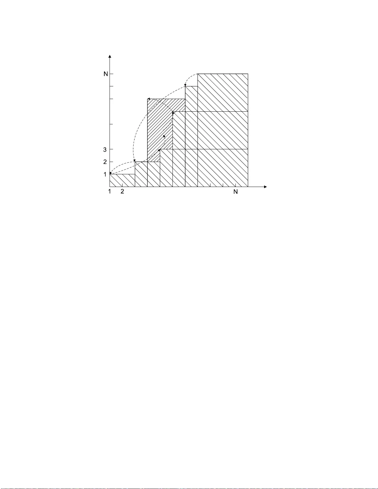
Side-informati on Scalable Source Coding Chao T ian, Member , IEEE , Suhas N. Diggavi, Member , IEEE Abstract The problem of side -informatio n scalable (SI-scalable) sourc e codin g is consid ered in this work, wh ere the encoder constru cts a pr ogressive description , such that the receiver with high quality side info rmation will be able to tru ncate the bitstream and reconstru ct in the rate distor tion sense, while the receiver with low quality side infor mation will have to receive fur ther data in o rder to deco de. W e pr ovide inner an d outer bo unds for general d iscrete m emoryless sour ces. The achievable region is shown to be tight for the ca se that eithe r o f the decoder s requires a lo ssless reconstructio n, as well a s th e case with d egraded dete rministic d istortion measures. Furthermo re we show that th e gap b etween the achievable r egion and the ou ter b ounds c an be boun ded by a constant when squ are error distortion measure is used . The notio n o f per fectly scalable coding is introd uced as both the stages op erate on the W yn er-Zi v b ound, and necessary and sufﬁcient co nditions a re giv en fo r sour ces satisfying a mild sup port condition . Using SI-scalable c oding and successi ve reﬁnem ent W yner-Ziv coding as basic building blocks, a co mplete characterization is provided fo r the impor tant q uadratic Gaussian sour ce with multiple jointly Gaussian side-in formation s, wher e th e side inform ation quality does no t h a ve to b e m onoton ic along the scalable coding o rder . Partial result is p rovided for the dou bly symmetric b inary sour ce with Hamm ing distortion wh en the worse side inform ation is a constan t, for which one of the o uter boun d is strictly tighter th an the oth er one. I . I N T R O D U C T I O N Consider the follo wing s cenario w here a se rver is to b roadcast multimedia d ata to multiple use rs with different side informations, howe ver the side informations are no t av a ilable a t the se rver . A user may h av e such strong side information that only minimal a dditional information is required from the server to satisfy a ﬁdelity criterion, or a user may have b arely any side information and expec t the server to provide virtually everything to satisfy a (possibly dif feren t) ﬁdelity criterion. A naive s trategy is to form a single des cription and broa dcast it to all the users, who can decod e only after receiving it completely re gardless o f the qua lity of their indi v idual s ide informations. Howe ver , for the use rs with good-qua lity side information (who will simply be referred to a s the good use rs), mo st of the information receiv ed is redu ndant, which introdu ces a delay cause d simply by the existence of use rs with poor-quality side informations (referred to as the bad u sers) in the network. It is natural to ask whe ther an o pportunistic method exists, i.e., whethe r it is possible to co nstruct a two-layer de scription, suc h that the go od use rs can decode with only the ﬁrst laye r , a nd the bad us ers receive both the ﬁrst and the seco nd layer to reconstruct. Moreover , it is of importanc e to in ves tigate wh ether such a coding o rder introduce s any performance loss . W e c all this c oding strategy side-information s calable (SI-sca lable) source coding, sinc e the scalable coding direction is from the 1 Encoder Decoder X 1 R 2 R 1 Y 2 Y 1 ˆ X 2 ˆ X Encoder Decoder 1 1 R 2 R 1 Y 2 Y 1 ˆ X 2 ˆ X Decoder 2 X Encoder Decoder 1 1 R 2 R 1 Y 2 Y 1 ˆ X 2 ˆ X Decoder 2 X 1 2 Y Y X l l 2 1 Y Y X l l Fig. 1. The SR-WZ system vs. the SI-scalable system. good us ers to the bad use rs. In this work, we c onsider mostly two-layer sys tems, except the quadratic Ga ussian source for wh ich the solution to the g eneral multi-layer prob lem is giv en. This work is related to the succe ssiv e reﬁnement prob lem, where a so urce is to b e encode d in a sca lable manner to satisfy different distortion requirement at e ach ind i vidu al s tage. T his problem was studied b y Koshelev [1], a nd by Equ itz an d C over [2]; a complete cha racterization of the rate-distortion region can be found in [3]. Ano ther related prob lem is the rate-distortion for sou rce coding with s ide information at the de coder [4], for wh ich W yn er and Ziv provided conc lusi ve result (now widely k nown as the W yn er -Ziv problem). Steinberg and Merhav [5] recently exten ded the succes siv e reﬁnemen t problem in the W yner -Zi v s etting (SR-WZ), wh en the s econd stage side information Y 2 is better than that of the ﬁrst stage Y 1 , in the s ense that X ↔ Y 2 ↔ Y 1 forms a Markov string. The extens ion to mu ltistage systems with degraded side informations in suc h a direction was recently completed in [6]. Also relevant is the work by Heegard a nd Berger [7] (see also [8]), wh ere the problem of source c oding when side information may be present a t the decod er was cons idered; the res ult was extended to the multistage case when the s ide informations a re degraded. T his is quite similar to the p roblem being conside red here an d in [5][6], howe ver without the scalable c oding requirement. Both the SR-WZ [5][6] and SI-sca lable problems can b e thought as spec ial ca ses of the problem of scalable source c oding w ith no s peciﬁc s tructure imposed on the de coder SI; this general problem appea rs to be q uite dif ﬁ cult, since even without the s calable req uirement, a complete solution to the problem has no t bee n found [7]. Here we e mphasize that the SR-WZ and the SI-scalable problem a re quite diff erent in terms o f their applications, though they seem similar since only the order of SI qu ality that is reversed. Roug hly s peaking, in the SI-scalab le 2 problem, the side information Y 2 at the later s tage is worse than the side information Y 1 at the early stag e, while in the SR-WZ problem, the order is rev ersed. In more ma thematically p recise terms, for the SI-scalable problem, the side informations are d egraded as X ↔ Y 1 ↔ Y 2 , in con trast to the S R-WZ problem where the reversed order is spe ciﬁed as X ↔ Y 2 ↔ Y 1 . The two problems are also different in terms of their p ossible app lications. The SR-WZ problem is more a pplicable for a sing le s erver -use r pair , when the u ser is receiving s ide information through an other c hannel, and a t the same time rec eivi ng the description(s) from the server; for this scen ario, two decode rs can be extracted to provide a simpliﬁed model. On the o ther hand, the SI-sca lable problem is more applicable when multiple use rs exist in the ne twork, and the server wants to provide a scalable de scription, s uch that the good us er is not jeopardize d unnece ssarily (se e Fig. 1). It is also worth pointing o ut that He egard and Berger showed whe n the s calable cod ing requirement is removed, the optimal encoding b y itself is in fact naturally prog ressiv e from the bad us er to the good one; as such, the SI- scalable problem is expected to b e more dif ﬁc ult tha n the SR-WZ problem, since the en coding orde r is reversed from the natural on e. This dif ﬁ culty is en capsulated by the fact that in the SR-WZ ordering the dec oder with better SI is able to deco de wha te ver message was meant for the dec oder with worse S I and henc e the ﬁrst stage can be max imally use ful. However , in the SI-sca lable p roblem an additional tension exists in the sense that the second -stage decode r will ne ed extra information to disambigua te the information of the ﬁrst stage . The problem is well understood for the lossless case. Th e key dif ference from t he lossy case is that the quality of the side informations can be n aturally determined by the value of H ( X | Y ) . By the seminal work of Slepian an d W olf [9], H ( X | Y ) is the minimum rate of en coding X losslessly with side information Y at the decode r , thus in a sen se a lar ger H ( X | Y ) c orresponds to weaker side information. If H ( X | Y 1 ) < H ( X | Y 2 ) , then the rate ( R 1 , R 2 ) = ( H ( X | Y 1 ) , H ( X | Y 2 ) − H ( X | Y 1 )) is achievable, a s noticed by Feder and Shulman [10]. Extending this obse rv a tion a nd a coding scheme in [11], Draper [12] propose d a uni versal incremental Slepian-W olf coding scheme when the distributi on is unkn own, wh ich inspired Eck ford and Y u [13 ] to d esign rateless Slep ian-W olf LDPC c ode. For the loss less case , the re is no loss of optimality by using a scalab le coding approach ; an immediate ques tion is to ask whether the sa me is true for the lossy cas e in terms of rate distortion, which we will show to b e n ot so in general. In this rate-distortion setting, the order of good ness b y the value of H ( X | Y ) is not suf ﬁcient b ecause of the presenc e of the distortion constraints. This moti vates the Markov condition X ↔ Y 1 ↔ Y 2 introduced for the SI-scalable coding problem. Going further alon g this point of view , the SI-sca lable problem is also app licable in the single user setting, when the source en coder does no t know exactly which side information the receiver has within a g i ven s et. The refore it c an be viewed as a s pecial case of the side-information universal rate d istortion cod ing. In this work, we formulate the problem of side information sc alable source coding, and provide two inner bounds a nd two outer bound s for the rate-distortion region. One of the inner- bounds has the sa me distortion and rate expressions as one of the ou ter bo unds, and they differ in the domain of optimization only by a Markov string requirement. Th ough the inner and the outer b ounds do no t co incide in gen eral, the inner boun ds are indeed tight for the ca se when either the ﬁrst stage or the sec ond sta ge requires a los sless reconstruction, as well as for the 3 case whe n certain deterministic distortion mea sures are taken. Furthermore, a c onclusive result is given for the quadratic Gaussian sou rce with any ﬁnite number o f stag es and arbitrary correlated Ga ussian side informations. W ith this s et o f inner and outer b ounds, the problem o f pe rfect scalability is in vestigated, deﬁned as when both of the layers can achieve the c orresponding W y ner -Zi v boun ds; this is s imilar t o the notion of (str ict) succe ssiv e reﬁna bility in the SR-WZ problem [5][6] 1 . Nece ssary and s uf ﬁ cient con ditions a re deriv ed for g eneral discrete memoryless s ources to be perfectly sc alable un der a mild s upport condition. By using the tool of rate- loss introduced by Zamir [14], we further s how that the gap betwee n the inner bounds and the outer boun ds are bound ed by a co nstant when squared error distortion measu re is us ed, and thus the inner bound s are “n early sufﬁcient”, in the s ense as giv e n in [15]. In addition to the result for the Gaussian so urce, partial result is p rovided for the dou bly symmetric binary source (DSBS) with Ha mming distortion mea sure when the seco nd s tage does n ot have side information, for which the inner bounds and outer bo unds co incide in certain dis tortion regimes. It is sh own one of the o uter bound c an be strictly better than the other for this s ource. The rest of the paper is organized as follows. In Section II we deﬁne the problem and establish the notation. In Section III, we provide inne r and outer bo unds to the rate-distortion region and s how tha t the boun ds co incide in certain s pecial case s. The n otion of perfectly sca lable is introduced in Section IV together with the example of a binary sou rce. The rate los s metho d is applied in Section V to show the gap between the inner bound and the outer bounds is bounde d. In VI, the G aussian so urce is treated within a more gene ral se tting. W e c onclude the paper in Sec tion VII. I I . N OTA T I O N A N D P R E L I M I N A R I E S Let X be a ﬁnite set and let X n be the s et of all n -vectors with compone nts in X . Den ote an a rbitrary me mber of X n as x n = ( x 1 , x 2 , . . . , x n ) , or a lternati vely a s x . Upper c ase is used for rand om variables and vectors. A discrete memoryles s source (DMS) ( X , P X ) is an inﬁn ite sequ ence { X i } ∞ i =1 of indep endent c opies of a random variable X in X wit h a gene ric distribution P X with P X ( x n ) = Q n i =1 P X ( x i ) . Similarly , let ( X , Y 1 , Y 2 , P X Y 1 Y 2 ) be a discrete memoryles s three-source with g eneric distribution P X Y 1 Y 2 ; the s ubscript will be dropped when it is clear from the con text as P ( X , Y 1 , Y 2 ) . Let ˆ X 1 and ˆ X 2 be ﬁnite reconstruction alph abets. L et d j : X × ˆ X j → [0 , ∞ ) , j = 1 , 2 be tw o distortion measures . The s ingle-letter distortion extension o f d j to vec tors is deﬁne d a s d j ( x , ˆ x ) = 1 n n X i =1 d j ( x i , ˆ x i ) , ∀ x ∈ X n , ˆ x ∈ ˆ X n j , j = 1 , 2 . (1) Deﬁnition 1: An ( n, M 1 , M 2 , D 1 , D 2 ) rate distortion (RD) SI-scalable code f or source X with side information 1 In the rest of the paper , decoder one, respectiv ely decoder two, will also be referred to as the ﬁrst stage decoder , respectiv el y second stage decoder , depending on the context. 4 ( Y 1 , Y 2 ) consis ts of two encod ing functions φ i and two dec oding functions ψ i , i = 1 , 2 : φ 1 : X n → I M 1 , φ 2 : X n → I M 2 , (2) ψ 1 : I M 1 × Y n 1 → ˆ X n 1 , ψ 2 : I M 1 × I M 2 × Y n 2 → ˆ X n 2 , (3) where I k = { 1 , 2 , . . . , k } , su ch that E d 1 ( X n , ψ 1 ( φ 1 ( X n ) , Y n 1 )) ≤ D 1 , (4) E d 2 ( X n , ψ 2 ( φ 1 ( X n ) , φ 2 ( X n ) , Y n 2 )) ≤ D 2 , (5) where E is the expec tation operation. Deﬁnition 2: A rate pair ( R 1 , R 2 ) is said to b e ( D 1 , D 2 ) -achiev ab le for SI-scalable encod ing with side information ( Y 1 , Y 2 ) , if for any ǫ > 0 and sufﬁciently large n , t here exist an ( n , M 1 , M 2 , D 1 + ǫ, D 2 + ǫ ) RD SI-scalable code, s uch that R 1 + ǫ ≥ 1 n log( M 1 ) a nd R 2 + ǫ ≥ 1 n log( M 2 ) . Denote the collection of all the ( D 1 , D 2 ) -achiev ab le rate p air ( R 1 , R 2 ) for SI-scalable enc oding a s R ( D 1 , D 2 ) , and we seek to charac terize this region whe n X ↔ Y 1 ↔ Y 2 forms a Ma rko v string (se e s imilar b ut dif fere nt degradedness cond itions in [5], [6]). Th e Mark ov co ndition in effect s peciﬁes t he goodness of the side informations . The ra te-distortion function for degraded side -informations was establishe d in [7] for the non-sca lable c oding problem. In light of the discus sion in Sec tion I, it gi ves a lower bound on the sum-rate for any RD SI-scalable code. More precisely , in order to ac hiev e d istortion D 1 with side information Y 1 , a nd ach ie ve dis tortion D 2 with side information Y 2 , when X ↔ Y 1 ↔ Y 2 , the rate-distortion func tion is R H B ( D 1 , D 2 ) = min p ( D 1 ,D 2 ) [ I ( X ; W 2 | Y 2 ) + I ( X ; W 1 | W 2 , Y 1 )] , (6) where p ( D 1 , D 2 ) is the set of all random variable ( W 1 , W 2 ) ∈ W 1 × W 2 jointly distributed with the generic random variables ( X , Y 1 , Y 2 ) , s uch that the follo wing conditions a re sa tisﬁed 2 : ( i ) ( W 1 , W 2 ) ↔ X ↔ Y 1 ↔ Y 2 is a Markov s tring; ( ii ) ˆ X 1 = f 1 ( W 1 , Y 1 ) a nd ˆ X 2 = f 2 ( W 2 , Y 2 ) s atisfy the distortion cons traints. Notice that the rate d istortion func tion R ( D 1 , D 2 ) giv e n above s uggests an en coding and decod ing o rder from the bad user to the good us er . W yner and Ziv [4] showed tha t un der the followi ng q uite gen eral ass umption tha t the distortion meas ure is chosen in the se t Γ d deﬁned as Γ d ∆ = { d ( · , · ) : d ( x, x ) = 0 , a nd d ( x, ˆ x ) > 0 if ˆ x 6 = x } , (7) then the rate distortion function satisﬁe s R ∗ X | Y (0) = H ( X | Y ) , where R ∗ X | Y ( D ) is the well-known W y ner- Z i v rate d istortion func tion with side information Y . If the s ame ass umption is made on the distortion measure 2 This form is slightly different from the one in [7] where f 1 was deﬁned as f 1 ( W 1 , W 2 , Y ) , but it is straightforwardly to verify that they are equiv alent. The cardinality bound is also ignored, which i s not essential here. 5 d 1 ( · , · ) ∈ Γ d , then we can eas ily show (using an a r g ument similar to the remark (3) in [4]) that R H B (0 , D 2 ) = min p ( D 2 ) [ I ( X ; W 2 | Y 2 ) + H ( X | W 2 , Y 1 )] , (8) where p ( D 2 ) is the s et of all ran dom variable W 2 such that W 2 ↔ X ↔ Y 1 ↔ Y 2 is a Markov string, and ˆ X 2 = f 2 ( W 2 , Y 2 ) s atisﬁes the distortion cons traint. I I I . I N N E R A N D O U T E R B O U N D S T o provide intuition into the the SI-sca lable problem, we ﬁrst examine a simple Gaus sian source under the mean squared e rror (MSE) distortion measu re, and describe the c oding sche mes informally . Let X ∼ N (0 , σ 2 x ) a nd Y 1 = Y = X + N , where N ∼ N (0 , σ 2 N ) is indepen dent of X ; Y 2 is simply a constan t, i.e., no side information at the sec ond dec oder . X ↔ Y 1 ↔ Y 2 is ind eed a Markov string. T o avoid lengthy discuss ion on dege nerate regimes, assume σ 2 N ≈ σ 2 x , and con sider only the following extreme case s. • σ 2 x ≫ D 1 ≫ D 2 : It is k nown binning with a Gau ssian c odebook, gene rated using a single-letter mech anism ( i.e., as an i.i.d. produ ct distributi on of the single-letter form) as W 1 = X + Z 1 , where Z 1 is a zero-mean Gaussian random variable ind ependen t of X su ch that D 1 = E [ X − E ( X | Y , W 1 )] 2 , is optimal for W yn er -Ziv coding. Th is coding scheme can still be us ed for the ﬁrst stage . In the secon d sta ge, by direct enu meration in the list of p ossible c odew ords in the p articular b in speciﬁed in the ﬁrst s tage, the exac t cod ew ord can be recovered by de coder two, who does not h av e any side information. Since σ 2 x ≫ D 1 ≫ D 2 , W 1 alone is not sufﬁcient to guarantee a distorti on D 2 , i.e., D 2 ≪ E [ X − E ( X | W 1 )] 2 . Thus a successive reﬁnement codebook, say us ing a Gaussian rand om variable W 2 conditioned on W 1 such that D 2 = E [ X − E ( X | W 1 , W 2 )] 2 , is needed . This lea ds to the achievable rates: R 1 ≥ I ( X ; W 1 | Y ) , R 1 + R 2 ≥ I ( X ; W 1 | Y ) + I ( W 1 ; Y ) + I ( X ; W 2 | W 1 ) = I ( X ; W 1 , W 2 ) . (9) • σ 2 x ≫ D 2 ≫ D 1 : If we choo se W 1 = X + Z 1 such that D 1 = E [ X − E ( X | Y , W 1 )] 2 and use the coding method in the previous case , then since D 2 ≫ D 1 , W 1 is su f ﬁc ient to achieve distortion D 2 , i.e., D 2 ≫ E [ X − E ( X | W 1 )] 2 . The rate ne eded for the e numeration is I ( W 1 ; Y ) , and it is rather wasteful sinc e W 1 is more than we need. T o solve this problem, we construct a coarser description using random vari able W 2 = X + Z 1 + Z 2 , such that D 2 = E [ X − E ( X | W 2 )] 2 . The enco ding proce ss has three e f fective layers for the nee ded two stage s: ( i ) the ﬁrst laye r use s W yner-Zi v coding with codewords gen erated by P W 2 ( ii ) the secon d layer uses s uccess i ve reﬁnement W yner-Zi v cod ing with P W 1 | W 2 ( iii ) the third lay er e numerates the spec iﬁc W 2 codeword within the ﬁrst laye r b in. Note that the ﬁrst two layers form a SR-WZ s cheme with identical side information Y at the de coder . For decoding, decode r one deco des the ﬁrst two laye rs with side information Y , while de coder two d ecodes the ﬁrst and the third layer without s ide information. 6 By the Markov s tring X ↔ W 1 ↔ W 2 , this s cheme gives the following rates: R 1 ≥ I ( X ; W 1 , W 2 | Y ) = I ( X ; W 1 | Y ) R 1 + R 2 ≥ I ( X ; W 1 | Y ) + I ( W 2 ; Y ) = I ( X ; W 2 ) + I ( X ; W 1 | Y , W 2 ) . (10) It is see n in the a bove discussion the speciﬁc coding sc hemes dep end on the d istortion values, which is not desirable since this usually sugges ts difﬁculty in proving the conv erse. T he two coding s chemes can be uniﬁed into a s ingle one by introducing an auxiliary ran dom variable, as will be shown in the se quel, however , it appe ars the con verse is indee d quite dif ﬁ cult to prove. In the rest of this s ection, inne r a nd outer b ounds for R ( D 1 , D 2 ) are provided. T he coding sche mes for the above Gaussia n example a re naturally generalized to give the inner bounds. It is further shown that the inner bounds are in fact tight for c ertain s pecial case s. A. T wo inn er bo unds Deﬁne the region R in ( D 1 , D 2 ) to be the se t of all rate pairs ( R 1 , R 2 ) for which the re exist random variables ( W 1 , W 2 , V ) in ﬁnite alphabets W 1 , W 2 , V such tha t the follo wing condition are satisﬁed. 1) ( W 1 , W 2 , V ) ↔ X ↔ Y 1 ↔ Y 2 is a Markov string. 2) There exist deterministic maps f j : W j × Y j → ˆ X j such tha t E d j ( X, f j ( W j , Y j )) ≤ D j , j = 1 , 2 . (11) 3) The non-negative rate pa irs sa tisfy: R 1 ≥ I ( X ; V , W 1 | Y 1 ) , R 1 + R 2 ≥ I ( X ; V , W 2 | Y 2 ) + I ( X ; W 1 | Y 1 , V ) . (12) 4) W 1 ↔ ( X, V ) ↔ W 2 is a Markov string. 5) The alphabe ts V , W 1 and W 2 satisfy |V | ≤ |X | + 3 , |W 1 | ≤ |X | ( |X | + 3) + 1 , |W 2 | ≤ |X | ( |X | + 3) + 1 . (13) The last two conditions can b e removed without ca using essential dif ference to the region R in ( D 1 , D 2 ) ; with them removed, n o spec iﬁc s tructure is requ ired on the joint distribution of ( X, V , W 1 , W 2 ) . T o see the last two conditions indee d d o not c ause loss of generality , a pply the s upport lemma [11] as follows. For a n arbitrary joint distrib u tion of ( X , V , W 1 , W 2 ) satisfying the ﬁrst three conditions, we ﬁrst red uce the cardinality of V . T o preserve P X and the two d istortions and two mutual information values, |X | + 3 letters are need ed. W ith this red uced alphabet, observe tha t b oth the distortion an d rate expressions depen d only on the marginal of ( X, V , W 1 ) and ( X, V , W 2 ) , respectively , hence requiring W 1 ↔ ( X, V ) ↔ W 2 being a Markov string does not c ause any loss of g enerality . Next to reduc e the c ardinality of W 1 , it is seen |X ||V | − 1 letters a re nee ded to p reserve the joint distrib u tion of ( X , V ) , o ne more is need ed to pres erve D 1 and another is nee ded to p reserve I ( X ; W 1 | Y 1 , V ) . 7 Fig. 2. An illustration of the codewo r ds in the nested binning structure. Thus |X | ( |X | + 3) + 1 letters sufﬁce. Note that we do not ne ed to prese rve the value of D 2 and the value of the other mutual information term bec ause of the aforementioned Markov s tring. A similar a r g ument holds for |W 2 | . The following the orem as serts that R in ( D 1 , D 2 ) is an ach ie vable region. Theore m 1: For any disc rete me moryless stochas tic source with s ide informations under the Markov co ndition X ↔ Y 1 ↔ Y 2 , R ( D 1 , D 2 ) ⊇ R in ( D 1 , D 2 ) . This theorem is proved in App endix II, and he re we o utline the c oding sc heme for this ac hiev able region in an intuiti ve mann er . The e ncoder ﬁ rst encod es using a V codebook with a “coarse ” binning, suc h tha t decod er one is able to dec ode it with s ide information Y 1 . A W yner-Zi v succ essive reﬁn ement c oding (with s ide information Y 1 ) is the n added co nditioned on the codeword V also for decode r one using W 1 . The en coder then enume rates the binn ing of V up to a level suc h that V is decoda ble by decod er two us ing the wea ker s ide information Y 2 . By doing so, decod er two is able to red uce the number of poss ible codewords in the (co arse) b in to a smaller number , which es sentially forms a “ ﬁner” b in; with the weaker side information Y 2 , the V code word is then decode d correctly with high probability . Another W yn er -Zi v succe ssiv e reﬁnemen t cod ing (with side information Y 2 ) is ﬁna lly ad ded cond itioned on the c odeword V for de coder two u sing a random code book of W 2 . As se en in the ab ove ar gument, in order to reduce the nu mber of po ssible V cod ew ords from the ﬁ rst stage to the se cond stage, the key idea is to c onstruct a nes ted binn ing structure as illustrated in F ig. 2. Note tha t this is a fundamen tally different from the code s tructure in SR-WZ, where no nested binn ing is nee ded. Each of the coarser bin contains the same numbe r of ﬁner bins; eac h ﬁn er bin holds ce rtain n umber o f codewords. They are constructed in such a way tha t g i ven the speciﬁc coa rser bin index, the ﬁrst stage deco der ca n decod e in it with the strong side information; at the s econd stage, a dditional bitstream is received b y the decode r , which further speciﬁes one of the ﬁner bin in the coarser bin, su ch that the se cond stag e dec oder can deco de in this ﬁner bin using the we aker side information. If we assign eac h c odew ord to a ﬁner bin independe ntly , then its co arser b in index is also ind ependen t o f that of the other codewords. W e note that the c oding sc heme d oes n ot explicitly require that side informations are degrad ed. Indeed as long as the chos en rand om variable V satisﬁes I ( V ; Y 1 ) ≥ I ( V ; Y 2 ) as well as the Markov co ndition, the region is 8 indeed ac hiev able. More precis ely , the following c orollary is straightforward. Corollary 1: For any d iscrete memoryless stoch astically so urce with side informations Y 1 and Y 2 (without the Markov structure), e R in ( D 1 , D 2 ) ⊆ R ( D 1 , D 2 ) , where e R in ( D 1 , D 2 ) is R in ( D 1 , D 2 ) with the additional condition that I ( V ; Y 1 ) ≥ I ( V ; Y 2 ) . W e c an sp ecialize the region R in ( D 1 , D 2 ) to giv e another inner bound. Let ˆ R in ( D 1 , D 2 ) be the se t of all rate pairs ( R 1 , R 2 ) for which there exist rand om variables ( W 1 , W 2 ) in ﬁ nite alphab ets W 1 , W 2 such tha t the follo wing c ondition are satisﬁed . 1) W 1 ↔ W 2 ↔ X ↔ Y 1 ↔ Y 2 or W 2 ↔ W 1 ↔ X ↔ Y 1 ↔ Y 2 is a Markov string. 2) There exist deterministic maps f j : W j × Y j → ˆ X j such tha t E d j ( X, f j ( W j , Y j )) ≤ D j , j = 1 , 2 . (14) 3) The non-negative rate pa irs sa tisfy: R 1 ≥ I ( X ; W 1 | Y 1 ) , R 1 + R 2 ≥ I ( X ; W 2 | Y 2 ) + I ( X ; W 1 | Y 1 , W 2 ) . (15) 4) The alphabe ts W 1 and W 2 satisfy |W 1 | ≤ ( |X | + 3)( |X | ( |X | + 3) + 1) , |W 1 | ≤ ( |X | + 3)( |X | ( |X | + 3) + 1) . (16) Corollary 2: For any discrete memoryless stoch astically source with side informations und er the Marko v condition X ↔ Y 1 ↔ Y 2 , R in ( D 1 , D 2 ) ⊇ ˆ R in ( D 1 , D 2 ) . The region ˆ R in ( D 1 , D 2 ) is particular interesting for the follo wing reasons . Firstly , it can be explicitly ma tched back to the coding scheme for the simple Ga ussian example. Sec ondly , it will be shown tha t one of t he outer bound s h as the same rate and distortion expres sions as ˆ R in ( D 1 , D 2 ) , only with a relaxed Markov s tring requirement. W e now prove this corollary . Pr oof of Cor ollary 2 When W 1 ↔ W 2 ↔ X , let V = W 1 . Then the rate express ions in Th eorem 1 giv es R 1 ≥ I ( X ; W 1 | Y 1 ) , R 1 + R 2 ≥ I ( X ; V , W 2 | Y 2 ) + I ( X ; W 1 | V , Y 1 ) = I ( X ; W 2 | Y 2 ) , (17) and therefore R in ( D 1 , D 2 ) ⊇ ˆ R in ( D 1 , D 2 ) for this c ase. When W 2 ↔ W 1 ↔ X , let V = W 2 . The n the rate expressions in Theorem 1 gi ves R 1 ≥ I ( X ; V , W 1 | Y 1 ) = I ( X ; W 1 | Y 1 ) R 1 + R 2 ≥ I ( X ; V , W 2 | Y 2 ) + I ( X ; W 1 | V , Y 1 ) = I ( X ; W 2 | Y 2 ) + I ( X ; W 1 | W 2 , Y 1 ) , and therefore R in ( D 1 , D 2 ) ⊇ ˆ R in ( D 1 , D 2 ) for this c ase. 9 The c ardinality b ound here is larger than that in Theorem 1 be cause of the req uirement to preserve the Markov conditions. B. T wo o uter bo unds Deﬁne the follo wing two regions, which will be sh own to be two o uter bounds . An obvious outer bound is giv e n by the intersection of the W yner- Zi v rate distortion function and the rate-distortion func tion for the problem considered by He egard an d Berger [7] with degrade d s ide information X ↔ Y 1 ↔ Y 2 R ∩ ( D 1 , D 2 ) = { ( R 1 , R 2 ) : R 1 ≥ R ∗ X | Y 1 ( D 1 ) , R 1 + R 2 ≥ R H B ( D 1 , D 2 ) } . (18) A tighter o uter b ound is now given as follows: deﬁne the region R out ( D 1 , D 2 ) to be the set of all rate pairs ( R 1 , R 2 ) for which there exist random variables ( W 1 , W 2 ) in ﬁ nite alphab ets W 1 , W 2 such tha t the following conditions are s atisﬁed. 1) ( W 1 , W 2 ) ↔ X ↔ Y 1 ↔ Y 2 . 2) There exist deterministic maps f j : W j × Y j → ˆ X j such tha t E d j ( X, f j ( W j , Y j )) ≤ D j , j = 1 , 2 . (19) 3) |W 1 | ≤ |X | ( |X | + 3) + 2 , |W 2 | ≤ |X | + 3 . 4) The non-negative rate vectors satisﬁes : R 1 ≥ I ( X ; W 1 | Y 1 ) , R 1 + R 2 ≥ I ( X ; W 2 | Y 2 ) + I ( X ; W 1 | Y 1 , W 2 ) . (20) The ma in res ult of this subs ection is the following the orem. Theore m 2: For a ny discrete memoryless stoc hastically sou rce with side informations under the Markov condition X ↔ Y 1 ↔ Y 2 , R ∩ ( D 1 , D 2 ) ⊇ R out ( D 1 , D 2 ) ⊇ R ( D 1 , D 2 ) . The ﬁrst inclusion of R ∩ ( D 1 , D 2 ) ⊇ R out ( D 1 , D 2 ) is obvious, s ince R out ( D 1 , D 2 ) takes the same form as R ∗ X | Y 1 ( D 1 ) and R H B ( D 1 , D 2 ) wh en the rates R 1 and R 1 + R 2 are co nsidered individually . T hus we will focus on the latter inclusion, whos e proof is gi ven in Appendix III . Note that the inne r bou nd ˆ R in ( D 1 , D 2 ) a nd R out ( D 1 , D 2 ) h av e the same rate an d distortion expressions an d they differ only by a Markov string req uirement (ignoring the non-ess ential cardinality bounds). Be cause of the dif fere nce in the d omain of optimizations, the two bounds may not produc e the same rate-regions. This is qu ite similar to the cas e of distrib uted loss y source cod ing p roblem, for wh ich the Berger -T ung inne r bound requ ires a long Markov string and the Berger -T u ng outer boun d requ ires only two short Markov s trings [16], but the ir rate and distortion expres sions are the s ame. 10 C. Loss less reconstruction a t one dec oder Since de coder one has better qu ality side inf ormation, it is reas onable for it to require a highe r quality reconstruction. Alternati vely , from the point of view of uni versal coding, when the encoder does not know the qua lity of the side information, it might as sume the be tter quality on e exists at the decode r and aim to reconstruct with a higher q uality , co mparing with the case when the poorer quality side information is av ailable. In the extreme case , deco der one might require a lossless reconstruction. In this subsec tion, we consider the setting where e ither decode r on e or deco der two re quires lossless rec onstruction. W e have the follo wing theorem. Theore m 3: If D 1 = 0 with d 1 ( · , · ) ∈ Γ d , or D 2 = 0 with d 2 ( · , · ) ∈ Γ d (see 7 for Γ d ), then R ( D 1 , D 2 ) = R in ( D 1 , D 2 ) . Mo re prec isely , for the former c ase, R (0 , D 2 ) = [ P W 2 ( D 2 ) { ( R 1 , R 2 ) : R 1 ≥ H ( X | Y 1 ) , R 1 + R 2 ≥ I ( X ; W 2 | Y 2 ) + H ( X | Y 1 , W 2 ) . } , (21) where P W 1 ( D 2 ) is the set of rando m vari ables s atisfying the Markov string W 2 ↔ X ↔ Y 1 ↔ Y 2 , and having a deterministic function f 2 satisfying E d ( f 2 ( W 2 , Y 2 ) , X ) ≤ D 2 . For the latter case , R ( D 1 , 0) = [ P W 1 ( D 1 ) { ( R 1 , R 2 ) : R 1 ≥ I ( X ; W 1 | Y 1 ) , R 1 + R 2 ≥ H ( X | Y 2 ) } , (22) where P W 1 ( D 1 ) is the set of rando m vari ables s atisfying the Markov string W 1 ↔ X ↔ Y 1 ↔ Y 2 , and having a deterministic function f 1 satisfying E d ( f 1 ( W 1 , Y 1 ) , X ) ≤ D 1 . Pr oof of T heorem 3: For D 1 = 0 , let W 1 = X and V = W 2 . The achievable rate vector implied by Theorem 1 is gi ven by R 1 ≥ H ( X | Y 1 ) , R 1 + R 2 ≥ I ( X ; W 2 | Y 2 ) + H ( X | Y 1 , W 2 ) . (23) It is seen that this rate region is tight by the c on verse of S lepian-W olf c oding for rate R 1 , and by (8) of Heegard- Berger coding for rate R 1 + R 2 . For D 2 = 0 , let W 1 = V and W 2 = X . The ac hiev able rate vector implied by Theorem 1 is giv en by R 1 ≥ I ( X ; W 1 | Y 1 ) , R 1 + R 2 ≥ H ( X | Y 2 ) . (24) It is eas ily seen that this rate region is tight by the con verse of W y ner- Zi v coding for rate R 1 , and the co n verse of Slepian-W o lf coding (or more precisely , W yner- Z i v rate d istortion function R X | Y 2 (0) with d 2 ( · , · ) ∈ Γ d as giv e n in [4]) for rate R 1 + R 2 . Zero distortion under a distortion me asure d ∈ Γ d can be i nterpreted as los sless , howev er , it is a we aker requirement than that the bloc k error proba bility is arbitrarily sma ll. Nevert heless, R (0 , D 2 ) and R ( D 1 , 0) in (21) and (22) still provide valid outer bounds for the more stringent loss less deﬁnition. On the othe r ha nd, it is rather s traightforw ard to spe cialize the c oding sche me for thes e cases , a nd show that the same conclusion is true for loss less cod ing in the this case . Thu s we have the following c orollary . 11 Corollary 3: The rate region, when the ﬁrst stage, and respec ti vely the secon d stage, requ ires los sless in terms of a rbitrary small block error probab ility is g i ven b y (21), res pectiv e ly (22), The key diff erence from the g eneral case whe n both stag es are loss y is the elimination of the need to gene rate one of code books using an auxiliary random variables, which s impliﬁes the matter tremendou sly . For exa mple when D 2 = 0 , sinc e the ﬁrst stage en coder gu arantees that w 1 and x are jointly typical, the secon d stage only needs to construct a c odebook o f x b y b inning the a pproximately 2 H ( X | W 1 ) such x vec tor directly . Subsequ ently the sec ond stage e ncoder does not se arch for a vector x ∗ to be jointly typical with bo th w 1 and x , but instead just sen ds the bin index of the ob served source vector x directly . Alternati vely , it ca n be understood as bo th the encode r and deco der at the s econd s tage have a ccess to a side information vector w 1 , and thus a conditional Slepian-W olf coding with decode r s ide information Y 2 sufﬁces. D. Deterministic distor tion measu r e Another ca se of interes t is wh en some fun ctions of the sou rce X is req uired to be recon structed with arbitrary small d istortion in terms of Hamming distortion; see [17 ] for the co rresponding cas e for the multiple description problem. More p recisely , let Q i : X → Z i , i = 1 , 2 be two deterministic functions and d enote Z i = Q i ( X ) . Consider the case that decoder i se eks to r econs truct Z i with arbitrarily small Hamming distorti on 3 . Th e achiev able region R in is tight when the functions satisfy certain degraded ness condition as stated in the follo wing theorem. Theore m 4: Let the distortion measure be H amming distortion d H : Z i × Z i → { 0 , 1 } for i = 1 , 2 . 1) If there exists a de terministic function Q ′ : Z 1 → Z 2 such that Q 2 = Q ′ · Q 1 , then R (0 , 0) = R in (0 , 0) . More precisely R (0 , 0) = { ( R 1 , R 2 ) : R 1 ≥ H ( Z 1 | Y 1 ) , R 1 + R 2 ≥ H ( Z 2 | Y 2 ) + H ( Z 1 | Y 1 Z 2 ) } . (25) 2) If there exists a de terministic function Q ′ : Z 2 → Z 1 such that Q 1 = Q ′ · Q 2 , then R (0 , 0) = R in (0 , 0) . More precisely R (0 , 0) = { ( R 1 , R 2 ) : R 1 ≥ H ( Z 1 | Y 1 ) , R 1 + R 2 ≥ H ( Z 2 | Y 2 ) } . (26) Pr oof of Theorem 4: T o prove (25), ﬁrst obs erve that b y letting W 1 = Z 1 and V = W 2 = Z 2 , R in clearly redu ces to the given expression. For the con verse, we start from the ou ter bou nd R out (0 , 0) , which implies that Z 1 is a function of W 1 and Y 1 , a nd Z 2 is a func tion of W 2 and Y 2 . For the ﬁrst stage rate R 1 , we have the following chain of e qualities R 1 ≥ I ( X ; W 1 | Y 1 ) = I ( X ; W 1 Z 1 | Y 1 ) ≥ I ( X ; Z 1 | Y 1 ) = H ( Z 1 | Y 1 ) − H ( Z 1 | X, Y 1 ) = H ( Z 1 | Y 1 ) . (27) 3 By a simil ar argument as i n the last subsection, the same result holds if block error probability is made arbitrarily small. 12 For the sum rate, we have R 1 + R 2 ≥ I ( X ; W 2 | Y 2 ) + I ( X ; W 1 | W 2 Y 1 ) = I ( X ; W 2 Z 2 | Y 2 ) + I ( X ; W 1 | W 2 Y 1 ) = I ( X ; Z 2 | Y 2 ) + I ( X ; W 2 | Y 2 Z 2 ) + I ( X ; W 1 | W 2 Y 1 ) = H ( Z 2 | Y 2 ) + I ( X ; W 2 | Y 2 Z 2 ) + I ( X ; W 1 | W 2 Y 1 ) ( a ) ≥ H ( Z 2 | Y 2 ) + I ( X ; W 2 | Y 1 Y 2 Z 2 ) + I ( X ; W 1 | W 2 Y 1 ) ( b ) = H ( Z 2 | Y 2 ) + I ( X ; W 2 | Y 1 Y 2 Z 2 ) + I ( X ; W 1 | W 2 Y 1 Y 2 ) = H ( Z 2 | Y 2 ) + I ( X ; W 2 | Y 1 Y 2 Z 2 ) + I ( X ; W 1 | W 2 Y 1 Y 2 Z 2 ) = H ( Z 2 | Y 2 ) + I ( X ; W 1 W 2 | Y 1 Y 2 Z 2 ) ≥ H ( Z 2 | Y 2 ) + I ( X ; Z 1 | Y 1 Y 2 Z 2 ) = H ( Z 2 | Y 2 ) + H ( Z 1 | Y 1 Y 2 Z 2 ) ( c ) = H ( Z 2 | Y 2 ) + H ( Z 1 | Y 1 Z 2 ) , where (a) is d ue to the Markov string W 2 ↔ X ↔ ( Y 1 Y 2 ) an d Z 2 is func tion of X ; (b) is du e to the Markov string ( W 1 W 2 ) ↔ X ↔ Y 1 ↔ Y 2 ; (c) is d ue to the Markov string ( Z 1 , Z 2 ) ↔ Y 1 ↔ Y 2 . Proof of p art 2) ( i.e., (26) relations hip) is straightforward an d is omitted. Clearly in the co n verse proof, t he requirement that the functions Q 1 and Q 2 are de graded is not need ed. Indeed this o uter bound ho lds for any general functions, however the degradednes s is needed for e stablishing the achiev ability of the region. If the c oding is not neces sarily sca lable, then it can be seen the sum rate is indeed achiev able, and the result above c an be used to establish a non-trivial special result in the context of the problem treated by He egard a nd Berger [7]. Corollary 4: Let the two function Q 1 and Q 2 be arbitrary , an d l et the distortion measure be Hamming distortion d H : Z i × Z i → { 0 , 1 } for i = 1 , 2 , then we h av e R H B (0 , 0) = H ( Z 2 | Y 2 ) + H ( Z 1 | Y 1 Z 2 ) . (28) I V . P E R F E C T S C A L A B I L I T Y A N D A B I N A RY S O U R C E In this sec tion we introduc e the notion of pe rfect scalab ility , which is deﬁned as whe n both the stag es operate at the W yner-Zi v rates. W e further examine the dou bly symmetric binary source and pro v ide a partial characterization and in vestigate its sca lability . The quadratic Gaus sian source with jointly Gaussian side informations is treated in S ection VI in a more general setting. A. P e rfect Sca lability The notion of the (strict) succ essive reﬁna bility deﬁned in [5] for the SR -WZ problem with forward degradation in the side-informations (SI) can b e applied to the reversely degrade d c ase cons idered in this pap er . This is done 13 by introduc ing the notion of perfect scalab ility for the SI-sca lable problem deﬁne d below . Deﬁnition 3: A s ource X is s aid to be per fectly scalable for distortion pair ( D 1 , D 2 ) , with side informations under the Markov string X ↔ Y 1 ↔ Y 2 , if ( R ∗ X | Y 1 ( D 1 ) , R ∗ X | Y 2 ( D 2 ) − R ∗ X | Y 1 ( D 1 )) ∈ R ( D 1 , D 2 ) . Theore m 5: A s ource X with side informations under the Markov string X ↔ Y 1 ↔ Y 2 , for which ∃ y 1 ∈ Y 1 such tha t P X Y 1 ( x, y 1 ) > 0 for e ach x ∈ X , is perfectly sc alable for distortion pair ( D 1 , D 2 ) if and only if there exist random variables ( W 1 , W 2 ) a nd deterministic maps f j : W j × Y j → ˆ X j such tha t the following conditions hold s imultaneously: 1) R ∗ X | Y j ( D j ) = I ( X ; W j | Y j ) a nd E d j ( X, f j ( W 1 , Y j )) ≤ D j , for j = 1 , 2 . 2) W 1 ↔ W 2 ↔ X ↔ Y 1 ↔ Y 2 forms a Markov string. 3) The alphabe t W 1 and W 2 satisfy |W 1 | ≤ |X | ( |X | + 3) + 2 , an d |W 2 | ≤ |X | + 3 . The Markov string is the most crucial condition, and the subs tring W 1 ↔ W 2 ↔ X is the same as one of the condition for succes si ve reﬁ nability without side information [2][3]. The support co ndition essen tially requ ires the existence of a worst letter y 1 in the a lphabet Y 1 such that it has no n-zero prob ability mass for each ( x, y 1 ) pair , x ∈ X . Pr oof of Theorem 5 The s uf ﬁ ciency being trivial, we only p rove the ne cessity . W ithou t loss of generality , ass ume P X ( x ) > 0 for all x ∈ X . By Theorem 2, if ( R ∗ X | Y 1 ( D 1 ) , R ∗ X | Y 2 ( D 2 ) − R ∗ X | Y 1 ( D 1 ) is ac hiev able for ( D 1 , D 2 ) , then using the tighter outer bou nd R out ( D 1 , D 2 ) of Theorem 2, there exist rando m variable W 1 , W 2 in ﬁn ite alphab et, whose sizes is bounded a s |W 1 | ≤ |X | ( |X | + 3) + 2 and |W 2 | ≤ |X | + 3 , and functions f 1 , f 2 such that ( W 1 , W 2 ) ↔ X ↔ Y 1 ↔ Y 2 is a Markov string, E d j ( X, f j ( W j , Y j )) ≤ D j for j = 1 , 2 and R ∗ X | Y 1 ( D 1 ) ≥ I ( X ; W 1 | Y 1 ) , R ∗ X | Y 2 ( D 2 ) ≥ I ( X ; W 2 | Y 2 ) + I ( X ; W 1 | Y 1 , W 2 ) . (29) It follo ws R ∗ X | Y 2 ( D 2 ) ≥ I ( X ; W 2 | Y 2 ) + I ( X ; W 1 | Y 1 , W 2 ) ≥ I ( X ; W 2 | Y 2 ) ( a ) ≥ R ∗ X | Y 2 ( D 2 ) , (30) where (a) follows t he con verse o f rate -distortion theorem for W yner-Zi v coding . Since the leftmost and the rightmost qua ntities are the same, all the inequa lities must be equa lities in (30), and it follows I ( X ; W 1 | Y 1 , W 2 ) = 0 . Similarly we h av e R ∗ X | Y 1 ( D 1 ) ≥ I ( X ; W 1 | Y 1 ) ≥ R ∗ X | Y 1 ( D 1 ) , (31) thus (31 ) also holds with equa lity . Notice that if W 1 ↔ W 2 ↔ X is a Markov string, then we ca n use Co rollary 2 to claim the sufﬁciency and complete the proof. Howe ver , this Markov c ondition is not true in gene ral. This is where the s upport condition is needed . 14 For conv enience, deﬁne the set F ( w 2 ) = { x ∈ X : P ( x, w 2 ) > 0 } . (32) By the Markov string ( W 1 , W 2 ) ↔ X ↔ Y 1 , the joint distrib u tion of ( w 1 , w 2 , x, y 1 ) ca n be factorized as follo ws P ( w 1 , w 2 , x, y 1 ) = P ( x, y 1 ) P ( w 2 | x ) P ( w 1 | x, w 2 ) . (33) Furthermore, I ( X ; W 1 | Y 1 , W 2 ) = 0 implies the Markov string X ↔ ( W 2 , Y 1 ) ↔ W 1 , and thus the joint distrib u tion o f ( w 1 , w 2 , x, y 1 ) c an also be factorized as follows P ( w 1 , w 2 , x, y 1 ) = P ( x, y 1 , w 2 ) p ( w 1 | y 1 , w 2 ) ( a ) = P ( x, y 1 ) P ( w 2 | x ) P ( w 1 | y 1 , w 2 ) , (34) where (a) follows by the Markov substring W 2 ↔ X ↔ Y 1 ↔ Y 2 . Fix an arbitrary ( w ∗ 1 , w ∗ 2 ) pair , by the assumption tha t P ( x, y 1 ) > 0 for a ny x ∈ X , we have P ( w ∗ 2 | x ) P ( w ∗ 1 | x, w ∗ 2 ) = P ( w ∗ 2 | x ) P ( w ∗ 1 | y 1 , w ∗ 2 ) (35) for any x ∈ X . Thus for any x ∈ F ( w ∗ 2 ) (se e deﬁnition in (32)) such that P ( w 1 | x, w ∗ 2 ) is we ll deﬁned , we have p ( w ∗ 1 | y 1 , w ∗ 2 ) = p ( w ∗ 1 | x, w ∗ 2 ) (36) and it further implies p ( w ∗ 1 | w ∗ 2 ) = P x P ( x, w ∗ 1 , w ∗ 2 ) P x P ( x, w ∗ 2 ) = P x ∈ F ( w ∗ 2 ) P ( x, w ∗ 2 ) P ( w ∗ 1 | y 1 , w ∗ 2 ) P x P ( x, w ∗ 2 ) = p ( w ∗ 1 | y 1 , w ∗ 2 ) = p ( w ∗ 1 | x, w ∗ 2 ) (37) for any x ∈ F ( w ∗ 2 ) . This indeed implies W 1 ↔ W 2 ↔ X is a Markov string, which completes the p roof. B. The Doubly Symmetric Binary Source with Hamming Distortion Measure Consider the following s ource: X is a me moryless b inary s ource X ∈ { 0 , 1 } and P ( X = 0) = 0 . 5 . The ﬁrst stage side information Y can be taken as the output of a bina ry symmetric chann el with input X , and cross over probability p < 0 . 5 . Th e sec ond stag e does not have side information. This source clearly satisﬁes the suppo rt condition in Theorem 5. It will be sh own that for some distortion pairs, this source is perfectly s calable, while for othe rs this is not poss ible. W e next ﬁrst provide partial results using ˆ R in and R ∩ previously gi ven . An explicit calculation of R H B ( D 1 , D 2 ) , together with the op timal forward tes t cha nnel s tructure, was given in a recent work [6]. W ith this explicit calculation, it c an be shown that in the sha ded region in Fig. 3, the outer bound R ∩ ( D 1 , D 2 ) is in fact achiev able (as we ll as in Region II, III and IV ; howe ver these three regions a re degenerate ca ses, and will be igno red in wh at follows). Re call the de ﬁnition of the critical distortion d c in the W yner-Zi v problem for the DSBS source in [4] G ( d c ) d c − p = G ′ ( d c ) , where G ( u ) = h b ( p ∗ u ) − h b ( u ) , h b ( u ) is the binary e ntropy function h b ( u ) = − u log u − (1 − u ) log (1 − u ) , 15 Region I-A 1 D 2 D c D c D Region I-D Fig. 3. The partition of the distortion region, where d c is the critical distorti on in [4] belo w which time sharing is not necessary . BSC BSC BSC Y X 1 W 2 W Fig. 4. The forward test channel in Region I-D. The crossov er probability for the BS C between X and W 1 is D 1 , while the crossov er probability η for the BSC between W 1 and W 2 is such that D 1 ∗ η = D 2 . and u ∗ v is the binary c on volution for 0 ≤ u, v ≤ 1 as u ∗ v = u (1 − v ) + v (1 − u ) . It was s hown in [4] that if D ≤ d c , then R ∗ X | Y ( D ) = G ( D ) . W e will use the following res ult from [6]. Theore m 6: For d istortion pairs ( D 1 , D 2 ) such that 0 ≤ D 2 ≤ 0 . 5 and 0 ≤ D 1 ≤ m in( d c , D 2 ) ( i.e., Region I-D), R H B ( D 1 , D 2 ) = 1 − h b ( D 2 ∗ p ) + G ( D 1 ) . This resu lt implies that for the shaded region I-D, the forward test cha nnel to a chieve this lower bound is in fact a cas cade of two BSC c hannels depicted in Fig. 4 . This choice clea rly s atisﬁes the cond ition in Co rollary 2 with the rates given by the outer bo und R ∩ ( D 1 , D 2 ) , which shows that this outer bound is indee d achievable. Note the following ineq uality R H B ( D 1 , D 2 ) = 1 − h b ( D 2 ∗ p ) + h b ( p ∗ D 1 ) − h b ( D 1 ) ≥ 1 − h b ( D 2 ) = R ( D 2 ) , (38) where the inequa lity is due to the mono tonicity of G ( u ) in 0 ≤ u ≤ 0 . 5 , we conclude that in this regime the source is no t pe rfectly scalable. T o s ee R ∩ ( D 1 , D 2 ) is also achiev a ble in region I-C, recall the res ult in [4] that the optimal forward test channe l to achieve R ∗ X | Y ( D ) ha s the following structure: it is the time-sharing between z ero-rate coding and a BSC with cros sover p robability d c if D ≥ d c , or a single BSC with crossover probability D o therwise. Thus it is straightforward to verify that R ∩ ( D 1 , D 2 ) is achiev able by time sharing the two forward test channels in Fig. 5; 16 BSC BSC BSC Y X 2 W 1 W (a) BSC BSC Y X 2 W (b) Fig. 5. The forward test channels in Region I-C . The crossov er probability for the BSC between X and W 2 is D 2 in both the channels, while the crossover probability η for the BSC between W 2 and W 1 in (a) is such that D 2 ≤ D 1 ∗ η = η ′ ≤ d c . Note for (b), W 1 can be taken as a constant. 0.1 0.105 0.11 0.115 0.12 0.125 0.11 0.115 0.12 0.125 0.13 0.135 0.14 0.145 0.15 R 1 R 2 R out (D 1 ,D 2 ) R ∩ (D 1 ,D 2 ) Fig. 6. The rate outer bounds f or a particular choice of D 1 , D 2 in Region I-B of Figure 3. furthermore, a n e quiv alent forward tes t channe l can b e found such that the Markov condition W ′ 1 ↔ W 2 ↔ X is satisﬁed, which s atisﬁes the c onditions giv en in The orem 5. Thus in this regime, the source is in fact pe rfectly scalable. Unfortunately , we were not a ble to ﬁnd the complete c haracterization for the regime I-A and I-B. Us ing an approa ch s imilar to [6], an explicit outer b ound can be d eri ved from R out ( D 1 , D 2 ) . It c an then be s hown numerically tha t for certain distortion pairs in this regime, R out ( D 1 , D 2 ) is strictly tighter than R ∩ ( D 1 , D 2 ) . This ca lculation ca n b e found in [18] and is omitted here. An example is g i ven in Fig. 6 for the two o uter boun ds with a n on-zero gap in between for a sp eciﬁc distortion pair in Region I-B. V . A N E A R S U FFI C I E N C Y R E S U L T By using the tool of rate loss introduced by Zamir [14], which was further developed in [15], [19]–[21 ], it can be shown tha t whe n both the sou rce an d recon struction alph abets are reals, and the distortion measure is 17 ) , ( 2 1 D D   ) , ( 2 1 D D out  ) , ( 2 1 D D in  1 R 2 R Fig. 7. An illustration of the gap between the inner bound and the outer bounds when MSE is the distortion measure. The two regions R in ( D 1 , D 2 ) and R out ( D 1 , D 2 ) are giv en in dashed lines, si nce it is unkno wn whether they are indeed the same. MSE, the g ap between the achievable region a nd the out bounds are bo unded by a cons tant. Thu s the inner and outer bound s a re nearly su f ﬁc ient in the sens e d eﬁned in [15]. T o show this res ult, we distinguish the two case s D 1 ≥ D 2 and D 1 ≤ D 2 . The s ource X is as sumed to have ﬁnite variance σ 2 x and ﬁnite (differential) entropy . The re sult of this sec tion is s ummarized in Fig. 7. A. The case D 1 ≥ D 2 Construct two random variable W ′ 1 = X + N 1 + N 2 and W ′ 2 = X + N 2 , whe re N 1 and N 2 are z ero mean independ ent Ga ussian random v ariables , i ndepen dent of everything els e, with v a riance σ 2 1 and σ 2 2 such that σ 2 1 + σ 2 2 = D 1 and σ 2 2 = D 2 . By letti ng V ′ = W ′ 1 , it is obvious that the follo wing rates are achiev ab le for distortion ( D 1 , D 2 ) from T heorem 1 R 1 = I ( X ; X + N 1 + N 2 | Y 1 ) , R 1 + R 2 = I ( X ; X + N 2 | Y 2 ) . (39) Let U be optimal rando m vari able to achiev e the W yner -Ziv rate at distortion D 1 giv e n decoder side information 18 Y 1 . Then it is clear that the dif ference between R 1 and the W y ner -Zi v rate c an be bou nded as, I ( X ; X + N 1 + N 2 | Y 1 ) − I ( X ; U | Y 1 ) ( a ) = I ( X ; X + N 1 + N 2 | U Y 1 ) − I ( X ; U | Y 1 , X + N 1 + N 2 ) ≤ I ( X ; X + N 1 + N 2 | U Y 1 ) = I ( X − ˆ X 1 ; X − ˆ X 1 + N 1 + N 2 | U Y 1 ) ≤ I ( X − ˆ X 1 , U, Y 1 ; X − ˆ X 1 + N 1 + N 2 ) = I ( X − ˆ X 1 ; X − ˆ X 1 + N 1 + N 2 ) + I ( U, Y 1 ; X − ˆ X 1 + N 1 + N 2 | X − ˆ X 1 ) = I ( X − ˆ X 1 ; X − ˆ X 1 + N 1 + N 2 ) ( b ) ≤ 1 2 log 2 D 1 + D 1 D 1 = 0 . 5 (40) where ( a ) is by applying chain rule to I ( X ; X + N 1 + N 2 , U | Y 1 ) in two diff erent ways; ( b ) is true becau se ˆ X 1 is the decoding function g i ven ( U, Y 1 ) , the distortion between X and ˆ X 1 is boun ded by D 1 , and X − ˆ X 1 is independ ent of ( N 1 , N 2 ) . Now we turn to bo und the g ap for the sum rate R 1 + R 2 . Le t W 1 and W 2 be the two random vari ables to achieve the rate d istortion function R H B ( D 1 , D 2 ) . First n otice the follo wing two identities d ue to the Markov string ( W 1 , W 2 ) ↔ X ↔ Y 1 ↔ Y 2 and ( N 1 , N 2 ) are ind ependen t of ( X , Y 1 , Y 2 ) I ( X ; W 2 | Y 2 ) + I ( X ; W 1 | W 2 Y 1 ) = I ( X ; W 1 W 2 | Y 1 ) + I ( Y 1 ; W 2 | Y 2 ) (41) I ( X ; X + N 2 | Y 2 ) = I ( X ; X + N 2 | Y 1 ) + I ( Y 1 ; X + N 2 | Y 2 ) . (42) Next we ca n bound the difference between the sum-rate R 1 + R 2 (as given in (39)) and the Heegard-Berger sum rate as follows. I ( X ; X + N 2 | Y 2 ) − I ( X ; W 2 | Y 2 ) − I ( X ; W 1 | W 2 Y 1 ) = { I ( X ; X + N 2 | Y 1 ) − I ( X ; W 1 W 2 | Y 1 ) } + { I ( Y 1 ; X + N 2 | Y 2 ) − I ( Y 1 ; W 2 | Y 2 ) } . ( 4 3) 19 T o bound the ﬁrs t bracket, notice that I ( X ; X + N 2 | Y 1 ) − I ( X ; W 1 W 2 | Y 1 ) = I ( X ; X + N 2 | W 1 W 2 Y 1 ) − I ( X ; W 1 W 2 | Y 1 , X + N 2 ) ≤ I ( X ; X + N 2 | W 1 W 2 Y 1 ) ( a ) = I ( X ; X + N 2 | W 1 W 2 Y 1 Y 2 ) = I ( X − ˆ X 2 ; X − ˆ X 2 + N 2 | W 1 W 2 Y 1 Y 2 ) ≤ I ( X − ˆ X 2 , W 1 , W 2 , Y 1 , Y 2 ; X − ˆ X 2 + N 2 ) = I ( X − ˆ X 2 ; X − ˆ X 2 + N 2 ) + I ( W 1 , W 2 , Y 1 , Y 2 ; X − ˆ X 2 + N 2 | X − ˆ X 2 ) = I ( X − ˆ X 2 ; X − ˆ X 2 + N 2 ) ≤ 1 2 log 2 D 2 + D 2 D 2 = 0 . 5 (44) where (a) is due to the Markov string ( W 1 , W 2 ) ↔ X ↔ Y 1 ↔ Y 2 , ˆ X 2 is the deco ding function given ( W 2 , Y 2 ) , and the o ther ineq ualities follow similar ar guments as in Eqn. (40). T o bound the sec ond brac ket, we write the follo wing I ( Y 1 ; X + N 2 | Y 2 ) − I ( Y 1 ; W 2 | Y 2 ) = I ( Y 1 ; X + N 2 | W 2 Y 2 ) − I ( Y 1 ; W 2 | Y 2 , X + N 2 ) ≤ I ( Y 1 ; X + N 2 | W 2 Y 2 ) ≤ I ( X Y 1 ; X + N 2 | W 2 Y 2 ) = I ( X ; X + N 2 | W 2 Y 2 ) ≤ 1 2 log 2 D 2 + D 2 D 2 = 0 . 5 (45) Thus w e have shown that for D 1 ≥ D 2 , the gap b etween the outer bound R ∩ ( D 1 , D 2 ) an d the inne r boun d R in ( D 1 , D 2 ) is bou nded. More precisely , the gap for R 1 is boun ded by 0.5 bit, while the ga p for the sum rate is bounded by 1 .0 bit. B. The case D 1 ≤ D 2 Construct random variable W ′ 1 = X + N 1 and W ′ 2 = X + N 1 + N 2 , where N 1 and N 2 are zero mea n independen t Gaussian rando m variables, independ ent of ev erything e lse, with v ariance σ 2 1 and σ 2 2 such that σ 2 1 = D 1 and σ 2 1 + σ 2 2 = D 2 . By letting V ′ = W ′ 2 = X + N 1 + N 2 , it is easily se en that the following rates are achiev able for distortion ( D 1 , D 2 ) R 1 = I ( X ; X + N 1 | Y 1 ) R 1 + R 2 = I ( X ; X + N 1 + N 2 | Y 2 ) + I ( X ; X + N 1 | Y 1 , X + N 1 + N 2 ) . Clearly , the argument for the ﬁrst s tage R 1 still holds with mino r c hanges. T o bound the s um-rate gap, notice 20 the follo wing identity I ( X ; X + N 1 + N 2 | Y 2 ) + I ( X ; X + N 1 | Y 1 , X + N 1 + N 2 ) = I ( X ; X + N 1 + N 2 | Y 1 ) + I ( Y 1 ; X + N 1 + N 2 | Y 2 ) + I ( X ; X + N 1 | Y 1 , X + N 1 + N 2 ) (46) = I ( Y 1 ; X + N 1 + N 2 | Y 2 ) + I ( X ; X + N 1 | Y 1 ) . (47) Next we see k to u pper bo und the following quantity I ( X ; X + N 1 + N 2 | Y 2 ) + I ( X ; X + N 1 | Y 1 , X + N 1 + N 2 ) − I ( X ; W 2 | Y 2 ) − I ( X ; W 1 | W 2 Y 1 ) = { I ( X ; X + N 1 | Y 1 ) − I ( X ; W 1 W 2 | Y 1 ) } + { I ( Y 1 ; X + N 1 + N 2 | Y 2 ) − I ( Y 1 ; W 2 | Y 2 ) } , ( 4 8) where a gain W 1 , W 2 are the R-D optimal ran dom variables for R H B ( D 1 , D 2 ) . For the ﬁrst bracket, we have I ( X ; X + N 1 | Y 1 ) − I ( X ; W 1 W 2 | Y 1 ) = I ( X ; X + N 1 | W 1 W 2 Y 1 ) − I ( X ; W 1 W 2 | Y 1 , X + N 1 ) ≤ I ( X ; X + N 1 | W 1 W 2 Y 1 ) = I ( X − ˆ X 1 ; X − ˆ X 1 + N 2 | W 1 W 2 Y 1 ) ≤ I ( X − ˆ X 1 , W 1 , W 2 , Y 1 ; X − ˆ X 1 + N 2 ) = I ( X − ˆ X 1 ; X − ˆ X 1 + N 1 ) + I ( W 1 , W 2 , Y 1 ; X − ˆ X 1 + N 1 | X − ˆ X 1 ) = I ( X − ˆ X 1 ; X − ˆ X 1 + N 1 ) ≤ 1 2 log D 1 + D 1 D 1 = 0 . 5 , (49) where ˆ X 1 is the decod ing function gi ven ( W 1 , Y 1 ) . For the second bracket, following a s imilar approach as (45), we have I ( Y 1 ; X + N 1 + N 2 | Y 2 ) − I ( Y 1 ; W 2 | Y 2 ) ≤ I ( X ; X + N 1 + N 2 | W 2 Y 2 ) ≤ I ( X − ˆ X 2 , W 2 , Y 2 ; X − ˆ X 2 + N 1 + N 2 ) = I ( X − ˆ X 2 ; X − ˆ X 2 + N 1 + N 2 ) ≤ 0 . 5 Thus we co nclude that for both c ases the gap between the inn er bound and the o uter bound is bo unded. Fig. 7 illustrates the inn er boun d and outer bounds , as we ll as the gap in be tween. V I . T H E Q U A D R AT I C G AU S S I A N S O U R C E W I T H J O I N T LY G AU S S I A N S I D E I N F O R M A T I O N S The degraded side information a ssumption, either X ↔ Y 1 ↔ Y 2 or X ↔ Y 2 ↔ Y 1 , for the quad ratic jointly Gaussian case is es pecially interesting, since phys ically degrade dness and stoc hastic degraded ness [22] do not cause essential difference in terms of the rate-distortion region for the problem being c onsidered [5]. Moreover , 21 jointly Gaussian so urce-side information is alw ays s tatistically degraded , the se forwardly a nd reversely degraded cases together p rovide a complete s olution to the jointly Gaussian case with two decode rs. In this section we in fact cons ider a more general setting with an arbitrary number of d ecoders for jointly Gaussian source and multiple side informations. Though the source and side informations c an hav e arbitrary correlation, in light o f the discus sion a bove, we will treat only physica lly degraded side informations. Note that since a speciﬁc enco ding order is spec iﬁed, thou gh the side informations are degraded as an un ordered set, the quality of s ide informations may not be monotonic along the scalab le coding order . Clearly the solution for the two stage cas e c an be red uced in a straightforward manne r from the gene ral solution. Recall from Theorem 2 (see (18)) that R ∩ ( D 1 , D 2 ) is an outer bo und derived from the interse ction of the Heegard-Berger and W yn er -Zi v bounds . T he generalization of the outer boun d R ∩ ( D 1 , D 2 ) to N dec oders plays a n important role, and the refore we take a detour in Section VI-A to start with the ch aracterization of R H B ( D 1 , D 2 , . . . , D N ) for the jointly Gaussian case. A. R H B ( D 1 , D 2 , . . . , D N ) for the jointly Gau ssian cas e Consider the following source X ∼ N (0 , σ 2 x ) , and side informations Y k = X + P k i =1 N i , whe re N i ∼ N (0 , σ 2 i ) are mutua lly indep endent an d independ ent of X . The result by Heegard and B er g er [7] gi ves R H B ( D 1 , D 2 , . . . , D N ) = min p ( D 1 ,D 2 ,...,D N ) N X k =1 I ( X ; W k | Y k , W k +1 , W k +2 , . . . , W N ) , (50) where p ( D 1 , D 2 , . . . , D N ) is the set of all ran dom variable with the Markov string ( W 1 , W 2 , . . . , W N ) ↔ X ↔ ( Y 1 , Y 2 , . . . , Y N ) , such that d eterministic functions f k ( Y k , W k , W k +1 , . . . , W N ) , k = 1 , . . . , N exist which satisfy the distortion cons traints. In [6], the cas e N = 2 was calculated explicitly , however such an explicit c alculation appears quite in volv ed for gene ral N due to the dis cussion of v a rious cases when some of the distortion constraints are not tight. In the sequel we approach the problem by showing a jointly Gaussian forw ard test channe l is optimal. Note that if we choo se to enforce only a subset of the distortion constraints, the rate for such a restriction gives a lower bound on R H B ( D 1 , D 2 , . . . , D N ) . By taking a ll the non-empty subs ets of the distortion co nstraints, labe led by eleme nts of I N = { 1 , 2 , . . . , N } , a total of 2 N − 1 lower bound s are av ailable and clearly the max imum of them is also a lower bound . More precis ely , we are interes ted in max R ∗ H B ( A D ) , where A D ⊆ I N and R ∗ H B ( A D ) is deﬁn ed in the se quel explicitly in terms of the distortion c onstraints on ly; note that if i ∈ A D , D i is still the distortion co nstraint for the de coder with s ide information Y i . W e next deriv e one of thes e lower b ounds using all the cons traints ( D 1 , D 2 , . . . , D N ) , i.e. A D = I N ; a s imilar de ri vation applies to the case with a ny subse t 22 A D ⊂ I N . Using (50) we have, N X k =1 I ( X ; W k | Y k , W k +1 , W k +2 , . . . , W N ) = h ( X | Y N ) − h ( X | Y 1 W N 1 ) − h ( X | Y N W N ) + h ( X | Y N − 1 W N ) − h ( X | Y N − 1 W N N − 1 ) + . . . + h ( X | Y 1 W N 2 ) ( a ) = h ( X | Y N ) − h ( X | Y 1 W N 1 ) − [ h ( X | Y N W N ) − h ( X | Y N − 1 Y N W N )] − . . . − [ h ( X | Y 2 W N 2 ) − h ( X | Y 1 Y 2 W N 2 )] = h ( X | Y N ) − h ( X | Y 1 W N 1 ) − I ( X ; Y N − 1 | Y N W N ) − I ( X ; Y N − 2 | Y N − 1 W N N − 1 ) − . . . − I ( X ; Y 1 | Y 2 W N 2 ) ( b ) = h ( X | Y N ) − h ( X | Y 1 W N 1 ) − [ h ( Y N − 1 | Y N W N ) − h ( Y N − 1 | X Y N )] − . . . − [ h ( Y 1 | Y 2 W N 2 ) − h ( Y 1 | Y 2 X )] = h ( X | Y N ) + N X k =2 h ( Y k − 1 | X Y k ) − N X k =2 h ( Y k − 1 | Y k W N k ) − h ( X | Y 1 , W N 1 ) , where (a) is bec ause of the Markov string X ↔ ( Y k − 1 W N k ) ↔ Y k , and (b) is becau se o f the Marko v string W N k ↔ ( X Y k ) ↔ Y k − 1 , both of which a re cons equenc es of W N k ↔ X ↔ Y k − 1 ↔ Y k . The ﬁrst two terms depend o nly on the source and distrib u tion P X Y 1 ...Y N , and w e now see k to boun d the latter two terms, for which we have h ( X | Y 1 W N 1 ) = h ( X − E ( X | Y W N 1 ) | Y W N 1 ) ≤ h ( X − E ( X | Y W N 1 )) ≤ h ( N (0 , D 1 )) = 1 2 log(2 π eD 1 ) , (51) where the sec ond ine quality is becaus e Gaus sian distribut ion maximizes the entropy for a gi ven second mo ment, and E ( X − E ( X | Y W N 1 )) 2 ≤ D 1 by the existen ce of the de coding function f 1 . Next deﬁne γ k = P k − 1 i =1 σ 2 i P k i =1 σ 2 i , k = 2 , 3 , ..., N . (52) and write the following Y k − 1 = X + k − 1 X i =1 N i = X + k − 1 X i =1 N i + γ k k X i =1 N i − γ k k X i =1 N i (53) = γ k ( X + k X i =1 N i ) + (1 − γ k ) X + [ k − 1 X i =1 N i − γ k k X i =1 N i ] (54) = γ k Y k + (1 − γ k ) X + [ k − 1 X i =1 N i − γ k k X i =1 N i ] (55) 23 Notice that E [ Y k ( k − 1 X i =1 N i − γ k k X i =1 N i )] = k − 1 X i =1 σ 2 i − γ k k X i =1 σ 2 i = 0 , (56) and Y k and ( P k − 1 i =1 N i − γ i P k i =1 N i ) a re jointly Gauss ian, which implies tha t they a re inde pendent. Fu rther - more b ecause ( P k − 1 i =1 N i − γ i P k i =1 N i ) is independ ent of X , the Marko v string ( Y 1 , Y 2 , . . . Y N ) ↔ X ↔ ( W 1 , W 2 , . . . , W N ) implies that it is also indepe ndent of ( W 1 , W 2 , . . . , W N ) . It follows h ( Y k − 1 | Y k W N k ) = h γ k Y k + (1 − γ k ) X + k − 1 X i =1 N i − γ k k X i =1 N i | Y k W N k ! (57) = h (1 − γ k ) X + k − 1 X i =1 N i − γ k k X i =1 N i | Y k W N k ! (58) = h (1 − γ k )( X − E ( X | Y k W N k )) + k − 1 X i =1 N i − γ k k X i =1 N i | Y k W N k ! (59) ≤ h (1 − γ k )( X − E ( X | Y k W N k )) + k − 1 X i =1 N i − γ k k X i =1 N i ! . (60) By the a forementioned indepe ndence relation, the variance of term in the brac ket is bou nded ab ove by ˆ D k ∆ = (1 − γ k ) 2 D k + (1 − γ k ) 2 k − 1 X i =1 σ 2 i + γ 2 k σ 2 k . (61) Deﬁne the following qu antities K 1 ∆ = h ( X | Y N ) = 1 2 log 2 π eσ 4 x σ 2 x + P N i =1 σ 2 i , (62) K k ∆ = h ( Y k − 1 | X Y k ) = 1 2 log 2 π eσ 4 k P k i =1 σ 2 i , k = 2 , 3 , . . . , N (63) Summarizing the b ounds in (51) and (60), we hav e R H B ( D 1 , D 2 , . . . D N ) ≥ 1 2 log Q N i =1 K i Q N i =1 ˆ D i ∆ = R ∗ H B ( I N ) , (64) where for con venienc e we deﬁne ˆ D 1 = D 1 . T o sho w that max A D ⊆{ D 1 ,D 2 ,...,D N } R ∗ H B ( A D ) is indeed a chiev ab le, construct the random variables ( W ∗ 1 , W ∗ 2 , . . . , W ∗ N ) as follo w s. Ass ume that D k ≤ E [ X − E ( X | Y k )] 2 for each k = 1 , 2 , . . . , N , beca use otherwise this distortion req uirement can be ignored completely . [Construction o f ( W ∗ 1 , W ∗ 2 , . . . , W ∗ N ) ] 1) For each k = 1 , 2 , . . . , N , determine the variance σ 2 Z k of a Ga ussian random variable Z k such that D k = E [ X − E ( X | Y k , X + Z k )] 2 . 2) Rank the variance o f σ 2 Z k in a n increa sing order , and let ω ( k ) de note the rank of σ 2 Z k . 24 3) Calculate σ 2 Z ′ 1 = σ 2 Z ω − 1 (1) , and σ 2 Z ′ k = σ 2 Z ω − 1 ( k ) − σ 2 Z ω − 1 ( k − 1) for k = 2 , 3 , . . . , N . 4) Construct a set of inde pendent zero-mean Gauss ian rand om variables ( Z ′ 1 , Z ′ 2 , . . . , Z ′ N ) to have vari ance σ 2 Z ′ k . 5) Construct a set o f rando m variables ( W ∗ 1 , W ∗ 2 , . . . , W ∗ N ) as W ∗ k = X + ω ( k ) X i =1 Z ′ k . (65) Next we show that this c onstruction of ( W ∗ 1 , W ∗ 2 , . . . , W ∗ N ) ac hiev e s one o f aforemen tioned lo wer boun ds and thus is an optimal forward test c hannel. Choose the se t A ∗ D = { k : ω ( k ) < ω ( j ) for all j > k } , and d enote the rank (in inc reasing order) of its element k as r ( k ) . Clearly by the c onstruction we have N X k =1 I ( X ; W ∗ k | Y k , W ∗ k +1 , W ∗ k +2 , . . . , W ∗ N ) = X k ∈ A ∗ D I ( X ; W ∗ k | Y k , W ∗ k +1 , W ∗ k +2 , . . . , W ∗ N ) = | A ∗ D | X j =1 I ( X ; W ∗ r − 1 ( j ) | Y r − 1 ( j ) , W ∗ r − 1 ( j +1) ) = h ( X | Y r − 1 ( | A ∗ D | ) ) − h ( X | W ∗ r − 1 ( | A ∗ D | ) Y r − 1 ( | A ∗ D | ) ) + h ( X | Y r − 1 ( | A ∗ D |− 1) W ∗ r − 1 ( | A ∗ D | ) ) − h ( X | Y r − 1 ( | A ∗ D |− 1) W ∗ r − 1 ( | A ∗ D |− 1) ) + . . . + h ( X | Y r − 1 (1) W ∗ r − 1 (2 ) − h ( X | Y r − 1 (1) W ∗ r − 1 (1) ) = h ( X | Y r − 1 ( | A ∗ D | ) ) − h ( X | Y r − 1 (1) W ∗ r − 1 (1) ) − [ h ( Y r − 1 ( | A ∗ D |− 1) | Y r − 1 ( | A ∗ D | ) W ∗ r − 1 ( | A ∗ D | ) ) − h ( Y r − 1 ( | A ∗ D |− 1) | X Y r − 1 ( | A ∗ D | ) )] − . . . − [ h ( Y r − 1 (1) | Y r − 1 (2) W ∗ r − 1 (2) ) − h ( Y r − 1 (1) | X Y r − 1 (2) )] = R ∗ H B ( A ∗ D ) becaus e of the construction of ( W ∗ 1 , W ∗ 2 , . . . , W ∗ N ) and the fact that they a re jointly Gaus sian with ( X, Y 1 , Y 2 , . . . , Y N ) . T hus, we have proved the following theorem. Theore m 7: The au xiliary ran dom variable ( W ∗ 1 , W ∗ 2 , . . . , W ∗ N ) con structed above achieves the minimum in the Heegard and Ber ger rate distortion fun ction for the jointly Ga ussian s ource a nd side informations. It is clear that we can determine the set A ∗ D before co nstructing ( W ∗ 1 , W ∗ 2 , . . . , W ∗ N ) us ing the aforementioned procedure, which can simplify the cons truction. Howe ver , the current construction has the advantage that eac h W ∗ k is a lmost individually determined by D k , a nd doe s not s ubstantially dep end on the othe r distortion constraints. This will p rov e to be useful for the general sca lable co ding problem. It is worth no ting that it seeming ly requ ires comparing 2 N − 1 values of R ∗ H B ( A D ) to determine R H B ( D 1 , D 2 , . . . , D 2 ) , ho wev er , from t he forw a rd calculation we se e that in fact O ( N ) complexity su f ﬁc es. This result can be interpreted us ing Fig. 8 . On the horizontal axis, the N marks stand for t he N random 25 N Y 1  N Y 2  N Y 3  N Y 1 Y 2 Y 3 Y k Y * ) ( 1 k W  Z j i R , Fig. 8. An illustration of the sum-rate for t he Gaussian case. variable ( W ∗ ω − 1 (1) , W ∗ ω − 1 (2) , . . . , W ∗ ω − 1 ( N ) ) , an d the on the vertical axis, the N marks stan d for the N levels o f side informations ( Y 1 , Y 2 , . . . , Y N ) . The ran dom variable pairs ( W k , Y k ) are then the points o f interest on the plane, since if the k -th dec oder has ( Y k , W k ) the desired distortion can be achieved; the ( W k , Y k ) pairs are in one-to-one c orresponden ce to the ( ω ( k ) , k ) pairs. Next we assoc iate the unit squa re be lo w and to the right of each integer point ( i, j ) is associate d with a rate of value R i,j = I ( W ω − 1 ( i ) ; Y j − 1 | Y j W ω − 1 ( i +1) ) (66) where we deﬁne W ω − 1 ( N +1) = ∅ , and Y 0 = X . For eac h k = 1 , 2 , . . . , N , if we cover the rectan gle below a nd to the right of ( ω ( k ) , k ) , then the sum rate a ssociated with the covered a rea is exactly R H B ( D 1 , D 2 , . . . , D N ) . W ith Fig. 8, the coding scheme can b e u nderstood as foll ows. The coding proceed s from Y N to Y 1 , i.e., from high to lo w on the vertical axis; the k -th step ( k -th dec oder) speciﬁe s an integer point ( ω ( k ) , k ) , which correspond s to a ( W k , Y k ) pair , on the ﬁgure, an d additional rate is req uired if the area below and to the right of this p oint indu ces new area to cover . This order is illustrated in Fig. 8 along the arrows. Note that k X j =1 R i,j = k X j =1 I ( W ω − 1 ( i ) ; Y j − 1 | Y j W ω − 1 ( i +1) ) (67) = k X j =1 [ I ( W ω − 1 ( i ) ; Y j − 1 | W ω − 1 ( i +1) ) − I ( W ω − 1 ( i ) ; Y j | W ω − 1 ( i +1) )] (68) = I ( W ω − 1 ( i ) ; X | W ω − 1 ( i +1) ) − I ( W ω − 1 ( i ) ; Y k | W ω − 1 ( i +1) )] (69) = I ( W ω − 1 ( i ) ; X | Y k W ω − 1 ( i +1) ) , (70) 26 and it is the rate for a vertical slice of h ight k be tween ho rizontal po sition i and i + 1 , which is in a quite similar form as (66). In this example ﬁgure, the decoders with side information Y N − 3 and Y 3 do not req uire additional rates. More generally , if ( ω ( k ) , k ) is ins ide the a rea already covered by the pre v ious coding step s ( N , N − 1 , . . . , k + 1) , then this stage do es not require a dditional rates. In fact, the c orners of the ﬁnal c overed area s peciﬁes the set A ∗ D . The follo wing obse rv ations are essen tial for the general Gaussian scalab le coding problem: each unit squa re in Fig. 8 is n ot me rely ass ociated with rate R i,j , it is in fact asso ciated with a fraction of cod e C i,j with the follo wing p roperties 1) The rate of C i,j is (asymptotically) R i,j ; 2) If the fractions of co de associated with the area be lo w and to the right of ( ω ( k ) , k ) are av ailable, then the decode r with side information Y k can decode within dis tortion D k ; 3) The same s et of code C i,j can b e use d to fulﬁll only subse t of the cons traints, the rate calculated by the covering area metho d is the quadratic Gaussian Heegard and Be r g er rate distortion function. The ﬁrst and s econd o bservations are straightforward by constructing the n ested b inning toge ther with conditional codebo oks as d escribed in Section III, i.e., N − 1 conditioning s tage from W ∗ ω − 1 (1) to W ∗ ω − 1 ( N ) and each conditioned codeb ook has N nested le vels from c oarse for Y 1 to ﬁne for Y N . In fact, it is not necess ary to use N nes ted level for ea ch codeboo k, but we do so for simplicity of un derstanding. The last prope rty is d ue to the inherent Ma rko v string amon g W ∗ 1 , W ∗ 2 , . . . , W ∗ N and X . B. Scalab le coding with joint Ga ussian side informations Now co nsider the sc alable coding problem whe re side informations and distortions are given by a permutation π ( · ) of that in the last sub section, i.e., Y ′ i = Y π ( i ) and D ′ i = D π ( i ) . W e next show that the identically permuted set of rand om variable ( W ∗ 1 , W ∗ 2 , . . . , W ∗ N ) achieves the Heegard-Berger rate distortion function for a ny ﬁrst k stages, thus optimal. In light of pictorial interpretation in Fig. 8, this reduce s to rearranging the co ded stream o f C i,j . Fig. 9 sh ows the effect of changing the scalable coding order . More precisely , for a certain s ide information Y ′ i = Y π ( i ) , deﬁ ne the followi ng sets: C ( k ) = { π ( i ) : i < k , π ( i ) > π ( k ) } (71) E − ( k ) = { π ( i ) : i < k , π ( i ) < π ( k ) , ω ( π ( i )) > ω ( π ( k )) } , (72) and the following function E ( k ) = max [ { π ( i ) : i < k , π ( i ) < π ( k ) , ω ( π ( i )) < ω ( π ( k )) } ∪ { 0 } ] , (73) and let Y 0 = X . Let the set of integers E − ( k ) b e o rdered inc reasingly , an d the rank of its eleme nt j be r ( j ) . Denote the set of random variables { W j : j ∈ C } as W ∗ C for an integer set C . T he follo wing k -th stage rate is 27 N Y 1  N Y 2  N Y 3  N Y 1 Y 2 Y 3 Y k Y * ) ( 1 k W  Z Fig. 9. An illustration of incremental rate for scalable coding. The denser shaded region gi ves the i ncremental rate R k for the stage with side information Y k . achiev able for k = 1 , 2 , . . . , N R k = | E − ( k ) | X i =1 I ( Y r − 1 ( i ) ; W ∗ r − 1 ( i ) | Y π ( k ) W ∗ r − 1 ( i +1) W ∗ r − 1 ( i +2) , . . . , W ∗ r − 1 ( | E − ( k ) | ) W ∗ C ( k ) ) + I ( Y E ( k ) ; W ∗ π ( k ) | Y π ( k ) W ∗ E − ( k ) W ∗ C ( k ) ) . It is clea rly this rate correspo nds to exa ctly the de nse sha ded region in Fig. 9, which is the s um of rates of fraction of c odes C ( i, j ) a s des cribed above. The property of this fraction co de C ( i, j ) thus implies the follo wing . Theore m 8: The Gaussian scalable coding ac hiev able rate region for distortion vector ( D π (1) , D π (2) , . . . , D π ( N ) ) is the rate vectors ( R 1 , R 2 , . . . , R N ) s atisﬁes k X i =1 R i ≥ R H B ( D π (1) , D π (2) , . . . , D π ( k ) ) , k = 1 , 2 , ..., N (74) where the side informations are ( Y π (1) , Y π (2) , . . . , Y π ( k ) ) . Fu rthermore, it is achievable by a jointly Gaussian codebo ok with ne sted binn ing. An immediate c onseque nce of this result is the following c orollary . Corollary 5: A d istortion vector ( D π (1) , D π (2) , . . . , D π ( N ) ) is perfectly scalab le along side informations ( Y π (1) , Y π (2) , . . . , Y π ( k ) ) for the jointly Gaussian source if an d on ly if R H B ( D π (1) , D π (2) , . . . , D π ( k ) ) = R ∗ X | Y π ( k ) ( D π ( k ) ) for e ach k = 1 , 2 , . . . , N . This corollary applies to one of the important sp ecial case s where D 1 = D 2 = . . . = D N and π ( k ) = N − k + 1 for eac h k , i.e., when all the deco ders have the same distortion requirement, and the scalable orde r is along a 28 decreas ing orde r of side information qua lity . Th is implies that at leas t for the Gaussia n ca se, an oppo rtunistic coding strategy does exist when the distortion req uirement is the same for all the users. V I I . C O N C L U S I O N W e s tudied the p roblem o f scalable source coding with reversely degraded side-information and gave two inn er bounds as well a s two outer boun ds. Th ese b ounds are tight for s pecial case s suc h as o ne lossless dec oder and under certain d eterministic distortion mea sures. Furthermore we provided a complete solution to the Gauss ian source with qu adratic distortion mea sure with any number of jointly Gaus sian side informations . The problem of perfect scalab ility is in ves tigated and the gap between the inne r and outer bounds are shown to be bounded . For the dou bly s ymmetric bina ry source with Ha mming distortion, we provided pa rtial results of the rate-distortion region. The res ult illustrates the diff erence b etween the lossless and the lossy so urce coding: thou gh a u ni versal approach exists with uncertain side informations at the dec oder for the lossles s case , such un certainty gen erally cause s los s of performance in the lossy case. A P P E N D I X I N O T AT I O N A N D B A S I C P RO P E RT I E S O F T Y P I C A L S E Q U E N C E S W e will f o llo w the deﬁnition of typica lity in [11], but use a slightly dif ferent n otation to make the small positiv e qua ntity δ explicit (see [5]). Deﬁnition 4: A se quence x ∈ X n is said to be δ -strongly-typical with res pect to a distrib ution P X ( x ) on X if 1) For a ll a ∈ X wi th P X ( a ) > 0     1 n N ( a | x ) − P X ( a )     < δ, (75) 2) For a ll a ∈ X wi th P X ( a ) = 0 , N ( a | x ) =0, where N ( a | x ) is the nu mber of occ urrences of the symbo l a in the s equenc e x . The set of seq uences x ∈ X n that is δ -strongly-typical is c alled the δ -strongly-typical se t and denoted as T δ [ X ] , where the dimens ion n is dropped. The following p roperties are well-known an d will be used in the proo f: 1) Giv en a x ∈ T δ [ X ] , for a y whose c omponent is drawn i.i.d a ccording to P Y and any δ ′ > δ , we have 2 − n ( I ( X ; Y )+ λ 1 ) ≤ P [( x , y ) ∈ T δ ′ [ X Y ] ] ≤ 2 − n ( I ( X ; Y ) − λ 1 ) (76) where λ 1 is a sma ll positive qua ntity λ 1 → 0 a s n → ∞ an d both δ, δ ′ → 0 . 2) Similarly , giv en ( x , y ) ∈ T δ ′ [ X Y ] , for any δ ′′ > δ ′ , let the co mponent o f z be drawn i.i.d according to the conditional mar ginal P Z i | Y i ( y i ) , the n 2 − n ( I ( X ; Z | Y )+ λ 2 ) ≤ P [( x , y , z ) ∈ T δ ′′ [ X Y Z ] ] ≤ 2 − n ( I ( X ; Z | Y ) − λ 2 ) (77) where λ 2 is a sma ll positive qua ntity λ 2 → 0 a s n → ∞ an d both δ ′ , δ ′′ → 0 . 29 3) Markov Lemma [16] : If X ↔ Y ↔ Z is a Markov string, a nd X and Y are s uch that their co mponent is drawn indepe ndently according to P X Y . Then for all δ > 0 lim n →∞ P [( X , z ) ∈ T |Y | δ [ X Z ] | ( Y , z ) ∈ T δ [ Y Z ] ] → 1 . (78) furthermore, lim n →∞ P [( X , Y , z ) ∈ T δ [ X Y Z ] | ( Y , z ) ∈ T δ [ Y Z ] ] → 1 . (79) A P P E N D I X I I P R O O F O F T H E O R E M 1 Codeboo k gene ration: Let a probability distribution P W 1 W 2 X Y 1 Y 2 = P X V W 1 W 2 P Y 1 | X P Y 2 | Y 1 , an d two reconstruction functions f 1 ( Y 1 , W 1 ) and f 2 ( Y 2 , W 2 ) be gi ven. First construct 2 nR A coarser bins and 2 nR A + R ′ A ﬁner bins, where R A and R ′ A are to be spec iﬁed later . Generate 2 R V length- n cod ew ords according to P V ( · ) , denote this set of codewords as C v ; as sign each of the m into o ne of the ﬁner bins indepen dently . For each c odeword v ∈ C v , generate 2 nR W 1 length- n codewords ac cording to P W 1 | V ( w 1 | v ) = Q n k =1 P W 1 | V ( w 1 ,k | v k ) , denote this set of codewords as C W 1 ( v ) ; ind ependen tly assign each codeword to o ne of the 2 nR B bins. Again for each V codeword, independ ently g enerate 2 nR W 2 length- n codewords ac cording to P W 2 | V ( w 2 | v ) = Q n k =1 P W 2 | V ( w 2 ,k | v k ) , denote this s et of c odew ords as C W 2 ( v ) ; independently assign eac h codeword to one of the 2 nR C bins. Reveal this codebo ok to the e ncoders and deco ders. Encoding: For a giv en x , ﬁn d in C v a codeword v ∗ such that ( x , v ∗ ) ∈ T 2 δ [ X V ] ; calculate the coarse r bin index i ( v ∗ ) , and the ﬁner bin index within the coarse r bin j ( v ∗ ) . Then in the C w 1 ( v ∗ ) codebook , ﬁnd a codew o rd w ∗ 1 such that ( w ∗ 1 , v ∗ , x ∗ ) ∈ T 3 δ [ W 1 V X ] , an d c alculate its corresp onding bin index k . In C w 2 ( v ∗ ) cod ebook, ﬁnd a co dew o rd w ∗ 2 such that ( w ∗ 2 , v ∗ , x ) ∈ T 3 δ [ W 2 V X ] , and calcu late its corresponding bin index l . The ﬁ rst-stage encode r se nds i and k , a nd the s econd-stag e encode r se nds j a nd l . In the ab ove p rocedure, if the re is more than one joint-typical se quence , ch oose the least; if there is no ne, choo se a d efault codeword and declare an error . Decoding: Th e ﬁrst stage decode r ﬁn ds ˆ v in the coa rser bin i , suc h that ( ˆ v , y 1 ) ∈ T 3 |X | δ [ V Y 1 ] ; the n in the C w 1 ( ˆ v ) codebo ok, ﬁnd ˆ w 1 such that ( ˆ w 1 , ˆ v , y 1 ) ∈ T 4 |X | δ [ W 1 V Y 1 ] . In the sec ond sta ge, the decod er ﬁn ds ˆ v in the ﬁne r b in speciﬁed by ( i, j ) such that ( ˆ v , y 2 ) ∈ T 3 |X | δ [ V Y 2 ] ; then in the C w 2 ( ˆ v ) co debook, ﬁnd ˆ w 2 such that ( ˆ w 2 , ˆ v , y 2 ) ∈ T 4 |X | δ [ W 2 V Y 2 ] . In the above procedure, if there is non e or there a re more than one, an error is declared and the deco ding stops. The ﬁrst d ecoder reco nstructs as ˆ x 1 ,k = f 1 ( ˆ w 1 ,k , y 1 ,k ) a nd the se cond decod er as ˆ x 2 ,k = f 2 ( ˆ w 2 ,k , y 2 ,k ) . Pr oba bility of e rr or: First d eﬁne the encod ing errors: E 0 = { X / ∈ T δ [ X ] } ∪ { Y 1 / ∈ T δ [ Y 1 ] } ∪ { Y 2 / ∈ T δ [ Y 2 ] } E 1 = E c 0 ∩ {∀ v ∈ C v , ( X , v ) / ∈ T 2 δ [ X V ] } E 2 = E c 0 ∩ E c 1 ∩ {∀ w 1 ∈ C w 1 ( v ∗ ) , ( w 1 , v ∗ , X ) / ∈ T 3 δ [ W 1 V X ] } E 3 = E c 0 ∩ E c 1 ∩ {∀ w 2 ∈ C w 2 ( v ∗ ) , ( w 2 , v ∗ , X ) / ∈ T 3 δ [ W 2 V X ] } . 30 Next deﬁne the decod ing errors: E 4 = E c 0 ∩ E c 1 ∩ { ( v ∗ , X , Y 1 ) / ∈ T 2 δ [ V X Y 1 ] } E 5 = E c 0 ∩ E c 1 ∩ { ( v ∗ , X , Y 2 ) / ∈ T 2 δ [ V X Y 2 ] } E 6 = E c 0 ∩ E c 1 ∩ {∃ v ′ 6 = v ∗ : i ( v ′ ) = i ( v ∗ ) a nd ( v ′ , Y 1 ) ∈ T 3 |X | δ [ V Y 1 ] } E 7 = E c 0 ∩ E c 1 ∩ {∃ v ′ 6 = v ∗ : i ( v ′ ) = i ( v ∗ ) a nd j ( v ′ ) = j ( v ∗ ) and ( v ′ , Y 2 ) ∈ T 3 |X | δ [ V Y 2 ] } E 8 = E c 0 ∩ E c 1 ∩ E c 2 ∩ E c 4 ∩ E c 6 ∩ { ( w ∗ 1 , v ∗ , X , Y 1 ) / ∈ T 3 δ [ W 1 V X Y 1 ] } E 9 = E c 0 ∩ E c 1 ∩ E c 3 ∩ E c 5 ∩ E c 7 ∩ { ( w ∗ 2 , v ∗ , X , Y 2 ) / ∈ T 3 δ [ W 2 V X Y 2 ] } E 10 = E c 0 ∩ E c 1 ∩ E c 2 ∩ E c 4 ∩ E c 6 ∩ {∃ w ′ 1 6 = w ∗ 1 : l ( w ′ 1 ) = l ( w ∗ 1 ) and ( w ′ 1 , v ∗ , Y 1 ) ∈ T 4 |X | δ [ W 1 V Y 1 ] } E 11 = E c 0 ∩ E c 1 ∩ E c 3 ∩ E c 5 ∩ E c 7 ∩ {∃ w ′ 2 6 = w ∗ 2 : l ( w ′ 2 ) = l ( w ∗ 2 ) and ( w ′ 2 , v ∗ , Y 2 ) ∈ T 4 |X | δ [ W 2 V Y 2 ] } Apparently , for any ǫ ′ , for n > n 1 ( ǫ ′ , δ ) , P ( E 0 ) ≤ ǫ ′ . W e h av e also P ( E 1 ) ≤ P ( X ∈ T δ [ X ] ) P ( {∀ v ∈ C v , ( X , v ) / ∈ T 2 δ [ X V ] }| X ∈ T δ [ X ] ) ≤ X x ∈ T δ [ X ] P X ( x )(1 − 2 − n ( I ( X ; V )+ λ ) ) nR 1 ≤ exp( − 2 − n ( I ( X ; V )+ λ − R V ) ) , (80) where Property 1 ) of the typical sequen ces and (1 − x ) y < e − xy are used. Th us P ( E 1 ) → 0 , provided tha t R V > I ( X ; V ) + λ . P ( E 4 ) and P ( E 5 ) both tends to zero due to the Markov lemma; it req uires the con dition ( v ∗ , X ) ∈ T 2 δ [ V X ] to ho ld, wh ich is indeed so giv en E 1 does not happen . Similarly , both P ( E 8 ) an d P ( E 9 ) tend s to ze ro for the same reas on. Notice that if ( v ∗ , X , Y 1 ) ∈ T 2 δ [ V X Y 1 ] , then ( v ∗ , Y 1 ) ∈ T 3 |X | δ [ V Y 1 ] , thus v ∗ can be c orrectly deco ded if there is no othe r codewords in the sa me bin satisfying the typ icality test. Conditioned on E c 1 , we have ( X , v ) ∈ T 2 δ [ X V ] . Thus P ( E 2 ) ≤ X ( x , v ) ∈ T 2 δ [ X V ] P r ( x , v )(1 − 2 − n ( I ( X ; W 1 | V )+ λ ) ) nR 2 ≤ exp( − 2 − n ( I ( X ; W 1 | V )+ λ 2 − R 2 ) ) (81) where property 2) o f the typic al sequ ences is used . Thus P ( E 2 ) ten ds to ze ro provided R W 1 > I ( X ; W 1 | V ) + λ 1 . Similarly P ( E ′ 3 ) ten ds to zero provided R W 2 > I ( X ; W 2 | V ) + λ 2 . Conditioned on E c 1 , y 1 ∈ T δ [ Y 1 ] , since codeword in C v are generated independ ently ac cording to P U ( · ) P ( E 6 ) ≤ X v ∈C v 2 − nR A 2 − n ( I ( Y 1 ; V ) − λ 1 ) = 2 n ( R V − R A − I ( Y 1 ; V )+ λ 1 ) (82) where we hav e used property 2) of the typical sequences and the fact the bin to which v is assigned is independe nt. 31 Thus P ( E 6 ) → 0 provided tha t R A > R V − I ( Y 1 ; V ) + λ 3 . Similarly P ( E 7 ) → 0 provided that R A + R ′ A > R V − I ( Y 2 ; V ) + λ 4 . Conditioned on E c 4 , ( v ∗ , Y 1 ) ∈ T 2 |X | δ [ V Y 1 ] . Thus P ( E 10 ) ≤ 2 nR W 1 2 − nR B 2 − n ( I ( Y 1 ; W 1 | V ) − λ 3 ) = 2 n ( R W 1 − R B − I ( Y 1 ; W 1 | V )+ λ 3 ) (83) where property 3) of the typical seque nces is used. Thus P ( E 10 ) tends to z ero provided R B > R W 1 − I ( Y 1 ; W 1 | V ) + λ 5 . Similarly , P ( E 11 ) te nds to zero provided R C > R W 2 − I ( Y 2 ; W 2 | V ) + λ 6 . Thus the rates only ne ed to sa tisfy R 1 = R A + R B > I ( X ; V W 1 | Y 1 ) + λ ′ (84) R 1 + R 2 = R A + R ′ A + R B + R C > I ( X ; V W 2 | Y 2 ) + I ( X ; W 2 | V Y 1 ) + λ ′′ (85) where λ ′ and λ ′′ are both sma ll po siti ve quantities and vanish as δ → 0 and n → ∞ ; then P e ≤ P 11 i =0 P ( E i ) → 0 . I t only remains to show that the distortions cons traints are sa tisﬁed as well. When no error o ccurs, the n ( ˆ W 1 , X , Y 1 ) ∈ T 3 |V | δ [ W 1 X Y ] and ( ˆ W 2 , X , Y 1 ) ∈ T 3 |V | δ [ W 2 X Y ] . By standard ar gument using the deﬁn ition of the typical sequen ces, it c an be shown that d ( x , ˆ x 1 ) ≤ E d [ X, f 1 ( W 1 , Y 1 )] + ǫ ′ (86) where ǫ ′ = max( d ( x, ˆ x ))(3 |V × W 1 × X × Y 1 | δ + P e ) . Th us the distortion can b e made arbitrarily small by choosing sufﬁciently small δ and s uf ﬁciently large n . Similar a r gu ments holds for the second s tage decod er . This completes the p roof. A P P E N D I X I I I P R O O F O F T H E T H E O R E M 2 Assume the existence of ( n, M 1 , M 2 , D 1 , D 2 ) RD SI-scalable code, there exist encoding and decod ing functions φ i and ψ i for 1 = 1 , 2 . Denote φ i ( X n ) as T i . X − k will b e use d to d enote the vector ( X 1 , X 2 , . . . , X k − 1 ) a nd X + k to de note ( X k +1 , X k +2 , . . . , X n ) ; the s ubscript k will be droppe d when it is c lear from the context. The proof follo ws the same line as the con verse proof in [7]. The follo wing chain of inequa lities is stand ard (see pa ge 440 32 of [22 ]). Here we omit the small positi ve quan tity ǫ for simplicity . nR 1 ≥ H ( T 1 ) ≥ H ( T 1 | Y 1 ) = I ( X ; T 1 | Y 1 ) = n X k =1 I ( X k ; T 1 | Y 1 X − k ) = n X k =1 H ( X k | Y 1 X − k ) − H ( X k | T 1 Y 1 X − k ) = n X k =1 H ( X k | Y 1 ,k ) − H ( X k | T 1 Y 1 X − k ) ≥ n X k =1 I ( X k ; T 1 Y − 1 Y + 1 | Y k ) . (87) Next we boun d the sum rate a s follows n ( R 1 + R 2 ) ≥ H ( T 1 T 2 ) ≥ H ( T 1 T 2 | Y 2 ) = I ( X ; T 1 T 2 | Y 2 ) = I ( X ; T 1 T 2 Y 1 | Y 2 ) − I ( X ; Y 1 | T 1 T 2 Y 2 ) = n X k =1 [ I ( X k ; T 1 T 2 Y 1 | Y 2 X − ) − I ( X ; Y 1 ,k | T 1 T 2 Y 2 Y − 1 )] . Since ( X k , Y 2 ,k ) is inde pendent of ( X − , Y − 2 , Y + 2 ) , we have I ( X k ; T 1 T 2 Y 1 | Y 2 X − ) = I ( X k ; T 1 T 2 Y 1 Y − 2 Y + 2 X − | Y 2 ,k ) ≥ I ( X k ; T 1 T 2 Y 1 Y − 2 Y + 2 | Y 2 ,k ) (88) The Ma rkov c ondition Y 1 ,k ↔ ( X k , Y 2 ,k ) ↔ ( X − X + T 1 T 2 Y − 1 Y − 2 Y + 2 ) giv es I ( X ; Y 1 ,k | T 1 T 2 Y 2 Y − 1 ) = I ( X k ; Y 1 ,k | T 1 T 2 Y 2 Y − 1 ) . (89) Thus we have n ( R 1 + R 2 ) ≥ n X k =1 [ I ( X k ; T 1 T 2 Y 1 Y − 2 Y + 2 | Y 2 ,k ) − I ( X k ; Y 1 ,k | T 1 T 2 Y 2 Y − 1 )] = n X k =1 [ I ( X k ; T 1 T 2 Y − 1 Y 2 − Y + 2 | Y 2 ,k ) + I ( X k ; Y + 1 | T 1 T 2 Y 2 Y − 1 Y 1 ,k )] . (90) The d egradedness giv es Y 2 ,k ↔ Y 1 ,k ↔ ( X k , T 1 T 2 , Y − 1 Y − 2 Y + 2 ) , wh ich implies n ( R 1 + R 2 ) ≥ n X k =1 [ I ( X k ; T 1 T 2 Y − 2 Y + 2 Y − 1 | Y 2 ,k ) + I ( X k ; Y + 1 | T 1 T 2 Y − 2 Y + 2 Y − 1 Y 1 ,k )] . (91) Deﬁne W 1 ,k = ( T 1 Y − 1 Y + 1 ) a nd W 2 ,k = ( T 1 T 2 Y − 2 Y + 2 Y − 1 ) , b y which we have nR 1 ≥ n X k =1 I ( X k ; W 1 ,k | Y 1 ,k ) (92) n ( R 1 + R 2 ) ≥ n X k =1 [ I ( X k ; W 2 ,k | Y 2 ,k ) + I ( X k ; W 1 ,k | W 2 ,k Y 1 ,k )] . (93) 33 Therefore the Marko v condition ( W 1 ,k , W 2 ,k ) ↔ X k ↔ Y 1 ,k ↔ Y 2 ,k is true. Next introduce the time sharing random variable Q , which is indep endent o f the multisource, and un iformly distrib uted over I n . Deﬁ ne W j = ( W j,Q , Q ) , j = 1 , 2 . The existence of function f j follo ws by de ﬁning f 1 ( W 1 , Y 1 ) = ψ 1 ,Q ( φ 1 ( X ) , Y 1 ) (94) f 2 ( W 2 , Y 2 ) = ψ 2 ,Q ( φ 1 ( X ) , φ 2 ( X ) , Y 2 ) (95) which leads the fulﬁllment of the distortion c onstraints. It only remains to show both the bound can be written in s ingle letter form in W 1 , W 2 , which is straightforward follo wing the ap proach in (page 4 35 of) [22]. This completes the p roof for R out ( D 1 , D 2 ) ⊇ R ( D 1 , D 2 ) .  A C K N O W L E D G E M E N T The d iscussion with Emre T elatar is gratefully ackn owl edged. R E F E R E N C E S [1] V . N. Koshe lev , “Hierarchical coding of discrete sources, ” P r obl. P er ed. Inform. , vol. 16, no. 3, pp. 31–49, 1980. [2] W . H. R. Equitz and T . M. Cov er , “Successiv e reﬁnement of information, ” IEEE T rans. Information Theory , vol. 37, no. 2, pp. 269–27 5, Mar . 1991. [3] B. Ri moldi, “S uccessi ve reﬁ nement of information: Characterization of achiev able rates, ” IEEE T rans. I nformation Theory , vol. 40, no. 1, pp. 253–259, Jan. 1994. [4] A. D. W yner and J. Zi v , “The rate-distortion function for source cod ing with side information at the decoder , ” IEEE T rans. Information Theory , vol. 22, no. 1, pp. 1–10, Jan. 1976. [5] Y . Steinberg and N. Merhav , “On successiv e r eﬁnement for t he W yner-Zi v problem, ” IEEE Tr ans. Information Theory , vol. 50, no. 8, pp. 1636–1654, Aug. 2004. [6] C. Tian and S. Diggavi, “On multistage successiv e reﬁ nement for Wyner-Zi v source coding with degraded side information, ” in EPFL T ech nical Report , Jan. 2006. [7] C. Heegard and T . Berger , “Rate distortion when side information may be absent, ” IEE E T rans. Information Theory , vol. 31, no. 6, pp. 727–734, Nov . 1985. [8] A. Kaspi, “Rate-distortion when side-information may be present at the decoder , ” IEEE T rans. Information Theory , vol. 40, no. 6, pp. 2031–2034, Nov . 1994. [9] D. Slepian and J. K. W olf, “Noiseless coding of correlated information source, ” IEEE Tr ans. Information Theory , vol. 19, no. 4, pp. 471–48 0, Jul. 1973. [10] M. Feder and N. Shulman, “Source broadcasting with unkno wn amount of receiver side information, ” in Pro c. IE EE Information Theory W orkshop , Oct. 2002, pp. 127–130. [11] I. Csiszar and J. K orner , Information theory: coding theor ems for discr ete memoryless systems . Academic Press, New Y ork, 1981. [12] S. C. Draper , “Univ ersal incremental S lepian-Wolf coding, ” in Pr oc. 43rd Annual Allerton Confer ence on communication, contro l and computing , Sep. 2002. [13] A. Eckford and W . Y u, “Rateless Slepian-Wolf codes, ” in Pr oc. Asil omar confer ence on signals, systems and computers , Oct.-Nov . 2005. [14] R. Zamir , “The rate loss in the Wyner-Ziv problem, ” IEEE T rans. Information Theory , vol. 42, no. 6, pp. 2073–2084 , N ov . 1996. [15] L. A. Lastras and V . C astelli, “Near sufﬁcienc y of random coding for two descriptions, ” IEEE T rans. Information T heory , vol. 52, no. 2, pp. 618–695, Feb . 2006. 34 [16] T . Berger , “Multiterminal source coding, ” in Lectur e notes at CISM summer school o n the information theory appr oach to communications , 1977. [17] A. E. Gamal and T . M. Cover , “ Achie vable rates for multiple descriptions, ” IEE E Tr ans. Information Theory , vol. 28, no. 6, pp. 851–85 7, Nov . 1982. [18] C. T i an and S. Diggavi, “Si de information scalable source coding, ” in E PFL T echnical Report , Sep. 2006. [19] L. L astras and T . Berger , “ All sources are nearly successi vely reﬁ nable, ” IEEE Tr ans. Information T heory , vol. 47, no. 3, pp. 918–926, Mar . 2001. [20] H. Feng and M. Effros, “Improved bounds for the rate loss of multiresolution source codes, ” I EEE T rans. Information Theory , vol. 49, no. 4, pp. 809–82 1, Apr . 2003. [21] H. Feng and Q. Z hao, “On the rate loss of multiresolution source codes in t he W yner-Ziv setting, ” IE EE T rans. on Information Theory , vol. 52, no. 3, pp. 1164-1171 , Mar . 2006. [22] T . M. Cov er and J. A. Thomas, Elements of information theory . New Y ork: Wile y , 1991.

Side-information Scalable Source Coding

Original Paper

Comments & Academic Discussion

Leave a Comment

Original Paper

Related Papers

Comments & Academic Discussion

Leave a Comment