Degree Optimization and Stability Condition for the Min-Sum Decoder
The min-sum (MS) algorithm is arguably the second most fundamental algorithm in the realm of message passing due to its optimality (for a tree code) with respect to the {\em block error} probability \cite{Wiberg}. There also seems to be a fundamental…
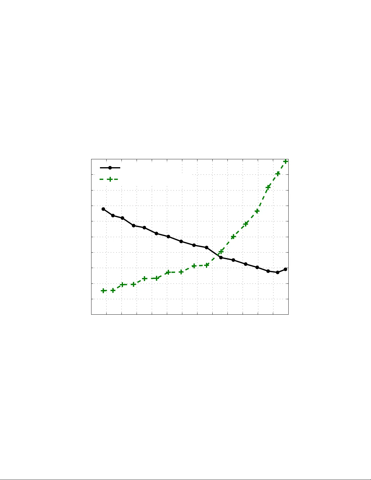
Authors: Refer to original PDF
De gree Optimizati on and Stability Condition for the Min-Sum Decoder Kapil Bhattad ECE Departmen t T exas A&M Uni versity College Station, TX 77843 kbhattad@ece. tamu.edu V ishwambhar Rathi School of Computer and Communica tion Sciences, EPFL Email: vishwambhar .rathi@epfl.ch Ruediger Urbanke School of Computer and Communica tion Sciences, EPFL Email: ruedig er .u rbanke@epfl.ch Abstract — The min-sum (MS) algorithm is ar guably the second most fundamental algorithm in the realm of message passing due to its optimality (for a tree code) with respect to the block error probability [1]. There also seems to be a fundamental relationship of MS decoding with the linear pr ogramming decoder [2]. Despite its importance, i ts fu ndamental properties ha ve not nearly been studied as well as those of the sum-product (also k nown as BP ) algorithm. W e address two questions related to the MS rule. First, we characterize the stability condition under MS decoding. It turns out to be essenti ally the same condition as under BP decoding. Second, we perfo rm a degree distribution opt imization. Contrary to the case of BP decoding, u nder MS decodin g th e th resholds of the best degree distributions f or standard irregular LDPC ensembles are significantly bounded away from the Shannon threshold. More precisely , on the A WGN channel, for the best codes that we find, the gap to capacity is 1 dB for a rate 0 . 3 code and it is 0 . 4 dB when the rate is 0 . 9 (the gap decrea ses monotonically as we in crease th e rate). W e also used the optimization p rocedure to design codes fo r modified M S algorithm wh ere the outpu t of the ch eck node is scaled by a constant 1 / α . For α = 1 . 25 , we observ ed th at the gap to capacity was lesser for th e modified MS algorithm wh en compared with th e MS algorithm. Howev er , it was still quite large, varying from 0.75 dB to 0.2 dB f or rates between 0.3 and 0.9. W e conclud e by p osing what we consider to be the most important open questions related to the M S algorithm. I . I N T RO D U C T I O N The min-sum (MS) decod er is perhap s th e second most fundam ental message passing decoder after Belief Prop agation (BP) decoder for two main reason s. Firstly , the MS de coder is optimal with respect to block erro r pro bability on a tree cod e [1]. Secondly , it is widely believed that the MS decoder is closely related to the linear p rogra mming (LP) b ased decoder propo sed in [12]. In [2], a complete characterization of the decodin g region of th e LP decoder h as bee n provide d with respect to the p seudocod ew ord s o f the underlying bipa rtite graph. The r esults in [13 ] suggest that the d ecoding region of the LP decoder is id entical to th at of the MS d ecoder (ind eed, this is the case fo r tree co des). In addition, the MS decoder is of practical interest becau se of its low implem entation complexity . In [11] , the asymptotic perform ance of th e MS deco der using density ev olution was ev aluated. Not much is kn own, howe ver , ana lytically abou t the den sity ev olution behavior of the MS d ecoder as co mpared to BP . W e first address the issue of stability of the MS decod er . In par ticular , we der iv e a co ndition which guaran tees that the densities correspon ding to the MS decoder which one observes in den sity ev olution co n verge to an “error-free” density . This condition turn s out to b e essentially the same as the stability condition fo r BP . Recall th at for the BP decode r the sp ace of de nsities wh ich arise in the context of d ensity evolution is the space of symmetric den sities. Unde r MS decod ing, on th e contr ary , no equiv alent condition is known. Empirically , one observes that for y ≥ 0 the d ensities fulfill the in equality a ( y ) e − y ≤ a ( − y ) ≤ a ( y ) . W e show that such a b ound indeed stays preserved unde r MS processing at the c heck n odes. The equiv alent question at the variable nodes is a n open question. What are the fundamental p erform ance limits und er M S decodin g? Un der BP deco ding an explicit optimization o f the degree distribution shows that we can seeming ly get arbitra rily close to capa city b y a p roper ch oice of the degree d istribution. Is the same behavior true under MS decoding or are the fundam ental limits which can not b e surpassed? In o rder to address this question we implemented an optimization tool based on EXIT charts. W e fo und th at the gap be tween th e best code an d Sh annon limit is r ather large. In [7] some simple improvements are proposed to the MS dec oder . For som e examp les, it is demon strated that by a simple scaling o f the output at the c heck nodes, the perfor mance of the MS decod er can be brough t closer to that of th e BP decoder . Using the LDPC co de d esign pro cedure, we also study how close we can get to the Sh annon capacity limit by using this m odified M S algorithm. The paper is organized as follows. In Section I I, we give relev ant definitio ns an d b riefly revie w the MS decod ing al- gorithm and its d ensity ev olutio n analy sis. In Section III, we derive a sufficient condition for stability and also discu ss some properties o f density which a rise in d ensity e volution. In Section IV, we discuss the optim ization procedu re. W e then present the op timization r esults in Section V and finally conclud e in Section VI . I I . D E FI N I T I O N S A N D P R E L I M I N A R I E S The LDPC ensemble is specified by specifyin g λ ( x ) = ∑ λ i x i − 1 and ρ ( x ) = ∑ ρ i x i − 1 which represent the degree d is- tribution ( dd) of the bit node s an d check nodes in the edge perspective, i.e., λ i ( ρ i ) is the fraction of edges connected to a degree i b it (ch eck) nod e. The design ra te of an LDPC ensemble is giv en b y 1 − ∑ ρ i i / ∑ λ i i . W e consider transm ission over a bin ary-inp ut, memory less, and symmetric (BMS) ch annel. Let L ch , u be the log- likelihood ratio ( LLR) of bit u obtained fr om the channel o bservation correspo nding to bit u . Le t L ( t ) cb , u , v and L ( t ) bc , u , v be the check to bit and bit to check m essage at iteration t correspondin g to edge ( u , v ) . W e will sometimes specifically refer to the binary input A WGN (biA WGN) chann el, Y = ( 1 − 2 X ) + N , where X ∈ { 0 , 1 } is th e input bit an d N has a Gaussian distribution with 0 m ean and variance σ 2 . In this case L ch is given by 2 Y / σ 2 and its distribution under the all zero co de word assumption is Gaussian with me an 2 / σ 2 and variance 4 / σ 2 . Finally , we denote th e Bhattacharyya constant as sociated to d ensity a b y B ( a ) = R ∞ − ∞ a ( x ) e − x 2 d x an d error p robab ility by P e ( a ) = R 0 − − ∞ a ( x ) d x + 1 2 R 0 + 0 − a ( x ) d x . W e now discuss the m essage passing rules f or the MS decoder . In MS d ecoder the bit to check message update is giv en by L ( t ) bc , u , v = L ch , u + ∑ v ′ : ( u , v ′ ) ∈ E , v ′ 6 = v L ( t − 1 ) cb , u , v ′ , (1) where E is the set of edges. The check to bit m essage update equation is L ( t ) cb , u , v = 1 α ∏ u ′ : ( u ′ , v ) ∈ E , u ′ 6 = u sgn ( L ( t ) bc , u ′ , v ) · min u ′ : ( u ′ , v ) ∈ E , u ′ 6 = u | L ( t ) bc , u ′ , v | . (2) For th e MS decode r α = 1 , but we will also co nsider modified MS decoder s with α > 1. The asymptotic per forman ce of LDPC co des u nder MS decodin g can be ch aracterized by stu dying the e volution of th e density o f the messages with iteratio ns (see [9]). Let a ch ( l ) , b t ( l ) , and a t ( l ) be the probability density functio n (pd f) of channel lo g-likelihood ratio, the me ssage fro m check to bit and bit to check node r espectively in t th iteration un der the all zero codeword assump tion. The den sity e volution equation for th e bit no de (correspo nd- ing to (1)) is gi ven by a t ( l ) = a ch ( l ) ⊛ ∑ λ i ( b t − 1 ( l )) ⊛ ( i − 1 ) (3) where a ⊛ i denotes conv olution o f a with itself i times. Sim- ilarly the check node side operation on densities is denoted by ⊠ . The pdf of the message at th e ou tput of ch eck nod es employing MS (corresp onding to (2)) has b een derived in [7 ], [11]. It is g iv en by 1 α b t l α , ρ ( a t ( l )) = ∑ ρ i i − 1 2 " ( a t ( l ) + a t ( − l )) Z ∞ | l | ( a t ( x ) + a t ( − x )) d x i − 2 + ( a t ( l ) − a t ( − l )) Z ∞ | l | ( a t ( x ) − a t ( − x )) d x i − 2 # . The den sity evolution pr ocess is started with b 0 ( l ) = δ 0 ( l ) and iterativ e decodin g is succe ssful if the densities ev entu ally ten d to δ ∞ ( l ) . I I I . S TA B I L I T Y C O N D I T I O N A N D S O M E P RO P E RT I E S O F T H E D E N S I T I E S In this section we de riv e the stability condition under MS decodin g. The stability cond ition gu arantees that if the den sity in density e volution r eaches “close” to error free d ensity ( δ ∞ ( l ) ) then it conv erges to it. W e derive th e stability conditio n by upper bo undin g the ev olution o f the Bhattach aryya parame- ter in den sity e volution. Note that the Bhattachar yya parameter appears n aturally in the context of BP wher e de nsities are symmetric. I n th is c ase the Bhattach aryya par ameter has a very concrete meaning: it is equal to − lim n → ∞ 1 n log ( P e ( a ⊛ n )) , where a is a symmetric d ensity . For g eneral densities which are not symmetric this is n o lo nger true but we can always com- pute B ( a ) = R ∞ − ∞ a ( x ) e − x 2 d x . Th e r eason we use Bha ttacharyy a parameter is to have a one dim ensional representation of densities and b ecause o f its p roper ty of being m ultiplicative on the variable node sid e. In the follo wing lem ma we g iv e a suf ficient co ndition for stability of δ ∞ ( l ) . This co ndition turns out to be same as the stability co ndition for BP (Theor em 5, [ 10]). Lemma 1 : Assume we are g iv en a degree distribution pair ( λ , ρ ) an d that transmission takes place over a BMS channel chara cterized by its L -density a ch . Define a 0 = a ch , and fo r t ≥ 1, defin e a t . = a ch ⊛ λ ( ρ ( a t − 1 )) = a ch ⊛ ∑ j λ j ∑ k ρ k ( a t − 1 ) ⊠ ( k − 1 ) ⊛ ( j − 1 ) . If B ( a ch ) λ ′ ( 0 ) ρ ′ ( 1 ) < 1 , (4) then there exists a strictly po siti ve c onstant ξ = ξ ( λ , ρ , a ch ) such that if , for some t ∈ N , B ( a t ) ≤ ξ , then B ( a t + n ) as well as P e ( a t + n ) conver ge to zero as n tends to infinity . Conversely , if B ( a ch ) λ ′ ( 0 ) ρ ′ ( 1 ) > 1 then lim inf t → ∞ P e ( a t ) > 0 with a 0 = a ch . Pr o of: By Lemma 3 in App endix we k now that B a ⊠ ( k − 1 ) t ≤ ( k − 1 ) B ( a t ) . Thus B ( a t + 1 ) = B ( a ch ) λ B ∑ k ρ k ( a t ) ⊠ ( k − 1 ) !! , ≤ B ( a ch ) λ ρ ′ ( 1 ) B ( a t ) . Expand ing the last eq uation around zero, we get = B ( a ch ) λ ′ ( 0 ) ρ ′ ( 1 ) B ( a t ) + O B ( a t ) 2 . Since B ( a ch ) λ ′ ( 0 ) ρ ′ ( 1 ) is assumed to be a constant less than 1, we can cho ose a sufficiently small ξ = ξ ( λ , ρ , a ch ) such that if B ( a t ) ≤ ξ , then B ( a ch ) λ ′ ( 0 ) ρ ′ ( 1 ) + O ( a t ) ≤ ε < 1. T herefor e if for some t ∈ N , B ( a t ) ≤ ξ , then B ( a t + n ) ≤ ε n B ( a t ) , wh ich conv erges to ze ro as n tends to infin ity . As P e ( a t + n ) = Z 0 − − ∞ a ( x ) d x + 1 2 Z 0 + 0 − a ( x ) d x ≤ Z 0 + − ∞ a ( x ) e − x 2 d x ≤ B ( a t + n ) , so P e ( a t + n ) also con verges to zer o. For the converse statement, the stability condition in Eqn (4) is a nece ssary cond ition f or BP deco ding to be successfu l. Hence by the optim ality of BP decodin g o n a tree it is also a necessary condition f or MS d ecoding to be successful. In proving th e sufficiency of the stability condition we used the Bhattachary ya p arameter as the fu nctional to project densities to on e dimen sion. However we could have u sed any other function al of the for m B α ( a ) = E e − α X , α > 0 which is m ultiplicative on th e variable no de side. Lemma 3 stays valid fo r a ny such fun ctional. Theref ore, we get a general stability condition that reads B α ( a ch ) λ ′ ( 0 ) ρ ′ ( 1 ) < 1. Howe ver , as a ch ( x ) is a symmetric density , B α ( a ch ) ≥ B ( a ch ) . This imp lies that th e sufficient co ndition fo r α 6 = 1 2 is we aker than the condition cor respond ing to Bha ttacharyya parame ter . Note that the co n verse in Lemma 1 is partial. It do es not say that the condition in Eqn (4) is necessary f or the den sity to con verge to δ ∞ ( l ) if f or some t the density a t is “close” to δ ∞ ( l ) . Howe ver the following ob servation sugg ests th at this indeed shou ld be the necessary conditio n. Su ppose we ev olve the density 2 εδ 0 ( l ) + ( 1 − 2 ε ) δ ∞ ( l ) und er th e MS decod er . Then it again f ollows by the a rguments of Theorem 5 in [10]) that for the density to con verge to δ ∞ ( l ) the necessary condition is B ( a ch ) λ ′ ( 0 ) ρ ′ ( 1 ) < 1. For the BP deco der we know th at 2 εδ 0 ( l ) + ( 1 − 2 ε ) δ ∞ ( l ) is the “best” d ensity (in the sense of d egradation) with erro r probab ility ε . Howe ver for th e MS deco der this is not the case. Hence we can not conclu de that Eqn(4) is a necessary con dition. The BP densities satisfy the symmetr y co ndition a ( x ) = a ( − x ) e x . The densities which arise in MS d ecoder do not satisfy the symmetry proper ty . Howe ver , we hav e ob served empirically tha t th e den sities satisfy the p roperty that a ( x ) ≥ a ( − x ) and a ( x ) ≤ a ( − x ) e x , x > 0. In th e following lemma we prove that these properties remain preserved on the check node side. Lemma 2 : Let a ( x ) and b ( x ) be two densities which satisfy the p roper ty that a ( x ) ≥ a ( − x ) , b ( x ) ≥ b ( − x ) and a ( x ) ≤ e x a ( − x ) , b ( x ) ≤ e x b ( − x ) for ∀ x > 0. Let c ( x ) = ( a ⊠ b )( x ) . Then c ( x ) ≥ c ( − x ) and c ( x ) ≤ e x c ( − x ) . Pr o of: L et A and B be random variables having d ensity a and b respectively . Th en c ( x ) = a ( x ) P ( B > | x | ) + b ( x ) P ( A > | x | ) + a ( − x ) P ( B < −| x | ) + b ( − x ) P ( A < −| x | ) . Thus c ( x ) − c ( − x ) = ( a ( x ) − a ( − x )) ( P ( B > x ) − P ( B < − x )) + ( b ( x ) − b ( − x )) ( P ( A > x ) − P ( A < − x )) , ≥ 0 . Similarly , c ( − x ) − e − x c ( x ) = a ( − x ) − e − x a ( x ) P ( B > x ) + b ( − x ) − e − x b ( x ) P ( A > x ) + a ( x ) − e − x a ( − x ) P ( B < − x ) + b ( x ) − e − x b ( − x ) P ( A < − x ) , which is g reater than or equal to zero by the assump tion. Proving L emma 2 for the variable node side is still an o pen question. I V . O P T I M I Z AT I O N P RO C E D U R E A. EXIT Charts EXIT charts [8 ] we re p roposed as a low comp lexity al- ternative to design and analy ze L DPC codes. T ypica lly b y assuming that the density of the messages exchang ed durin g iterativ e decod ing is Gaussian, the p roblem of code design can be red uced to a cur ve fitting prob lem which can b e done using linear programming . If the Gaussian assumption is exact, this technique is shown to be optimal in [6 ]. I n [ 3], a fast proced ure is p ropo sed th at uses a combin ation o f EXIT cha rts and d ensity evolution to design LDPC codes. The b asic id ea is to perform the design in steps, where, in each step, the LDPC co de en semble is optimize d using EXIT ch arts using the densities o f the messages ob tained from density ev olutio n of the ensem ble obtained in the pr evious step. In this paper , we u se a similar idea to design L DPC codes f or MS decod ing. An EXIT curve of a compo nent d ecoder is a p lot of the mutual in formatio n cor respond ing to the extrinsic o utput expressed as a f unction of the mutual infor mation co rrespon d- ing to the a priori input (message co ming fr om the o ther compon ent d ecoder) . Usually , it is assumed that the a priori informa tion is fro m an A WGN channel of signal-to- noise ratio 1 / σ 2 and the EXIT curve is obtaine d by calcu lating the input and output mutual information for σ 2 varying fro m 0 to ∞ . In an EXI T chart, the EXIT curves of one co mpon ent code and the flippe d EXIT cur ve of the o ther com ponen t code are plotted. Using this chart, we can pred ict the path taken by the iterativ e deco der as shown in Fig. 1. It has been observed that the actual path taken and the path predicted from EXIT charts are qu ite close. Based on this ob servation, LD PC cod es can be d esigned a s follows. Let I b ( I A , i ) ( I c ( I A , i ) ) b e mutual inform ation corresp onding to the extrinsic o utput of bit (check ) nod e of d egree i when the a pr iori mutual in formation is I A . The mu tual info rmation I can be calculated fro m the c ondition al distribution f ( l ) using I = Z ∞ − ∞ f ( l ) log 2 2 f ( l ) f ( l ) + f ( − l ) d l . (5) The EXIT curve o f the bit nodes a nd the check nodes is giv en b y I b = ∑ λ i I b ( I A , i ) and I c = ∑ ρ i I c ( I A , i ) respecti vely . Usually both I b and I c are increa sing fu nction o f I A . The con- vergence cond ition, based on the assumptio n o n th e message density , states th at the EXIT curve of the bit nodes should lie above that of the check n odes fo r the iterative decoder to con verge to the correc t co deword, i.e ., I b ( I A ) > I − 1 c ( I A ) or equiv alently I − 1 b ( I A ) < I c ( I A ) f or all I A where I c ( I − 1 c ( I A )) = I A . 0 0.1 0.2 0.3 0.4 0.5 0.6 0.7 0.8 0.9 1 0 0.1 0.2 0.3 0.4 0.5 0.6 0.7 0.8 0.9 1 I A in I E out I E in I A out EXIT chart (3,6) LDPC code Inner Decoder Outer Decoder 1.3dB Fig. 1: E XIT curves of the two componen t codes corresp onding to the (3,6) L DPC code transmitted over an A WGN chann el with E b / N 0 = 1 . 3 dB For a fixed ρ ( x ) , the pro blem of code design can th en be stated as the following linear prog ram max ∑ λ i / i subject to: ∑ λ i = 1 , λ i ≥ 0 , ∑ λ i I b ( I A , i ) > I − 1 c ( I A ) ∀ I A ∈ [ 0 , 1 ) . (6) Note th at maximizing the objective function corr esponds to maximizing the r ate. A similar linear pro gram can be written for optimizing ρ ( x ) for a giv en λ ( x ) . B. F ixed Chann el W e consider the problem of find ing LDPC co des for a given BMS channel such that reliable communication is possible with th e M S d ecoding algorithm. W e are in terested here in the perfor mance when the block length g oes to infinity . Our goa l is to maximize the r ate o f transmission. T owards achieving this goal we fir st pick an LDPC co de such tha t it conver ges to error free d ensity for the spe cified chann el. Starting from the in itial ensemble, the L DPC code ensem ble is optimized in several steps. In each step , the basic idea is to design the co des using EXIT ch arts. Howe ver , instead of usin g the Gaussian assumptio n on the inpu t d ensities, the inpu t den- sity in a p articular step of the o ptimization pr ocess is assume d to be the same as the d ensity ob tained by using the density ev olution proc edure for th e ensemble ob tained in the previous step. The inherent assumptio n is that the input den sities do not change muc h in one step of the optimiza tion procedure and the refore the approx imate EXIT cu rves obtain ed using the previous d ensities are close to the ac tual EXIT cur ves. No te that this assumption is different from the assumption that the density at iteratio n i for a particular o ptimization step is same as the density a t iteration i in the next op timization step. If we denote the densities at iteration i by a i and consider a family of densities that includes { γ a i + ( 1 − γ ) a i + 1 , γ ∈ [ 0 , 1 ] } then the assumption m ade is that the family of densities d oes not change much in on e step of the o ptimization. W e could sample many points in this f amily to enforce the condition in th e linear progr am th at the EXIT cur ves d o no t intersect. However , we sample only at p oints a i . This is u sually sufficient since if the old E XIT curves are close to each other , th en we get many samples ther e and at other points we have m ore leeway so we can sample fewer times. In each step of the optimization pr ocedur e, we gen erate a new d d pair from the p revious d d pair in two sub- steps. In the first sub-step we chang e λ ( x ) keeping ρ ( x ) constant and in the next sub-step we ch ange ρ ( x ) while keep ing λ ( x ) the same. The first sub-step is as follows. W e ch oose ρ ( x ) = ρ ol d ( x ) and o ptimize λ ( x ) as fo llows. W e perform den sity ev olutio n with the d d pa ir ( λ ol d , ρ ol d ) and at the end of each iteration store I l b ( d ) which is th e mutual inf ormation correspo nding to the e xtrin sic o utput of a bit node o f degree d at the end of iteration l . The optimizatio n th en reduces to the fo llowing linear progra m. max ∑ λ i / i ∑ λ i = 1 , λ i ≥ 0 , ∑ λ i i ≥ ∑ ρ i i , ∑ λ i I l b ( i ) > ∑ λ ol d , i I l − 1 b ( i ) + β ∑ λ ol d , i ( I l b ( i ) − I l − 1 b ( i )) β ∈ [ 0 , 1 ) ∀ l , (7) − δ ≤ λ i − λ ol d , i ≤ δ ∀ i , (8) λ 2 ≤ 1 B ( a ch ) ρ ′ ( 1 ) (from (4)) . (9) Before we explain the constraints, we note that the cost function cor respond s to maximizing the r ate and that the old dd pair satisfies the con straints a nd theref ore th e re sulting rate is a lways larger than the old rate. The Constraint (7) basically represents the condition that the EXIT curve correspo nding to the bit nodes should lie above that of the check nod es. The q uantity ∑ λ ol d , i ( I l b ( i ) − I l − 1 b ( i )) is the gap between the two EXIT curves cor respond ing to the old dd p air . The constant β determines how mu ch change in the ga p is allowed. If β is cho sen to be 0 the gap between the curves can beco me zer o w hile if β is cho sen to be one the gap is kept the same. By choosing a smaller β we weaken the con straints and therefor e get a larger rate. Howe ver , since the dd p air ch anges, the inpu t densities also change and therefo re the ac tual EXIT curves chang e. Since the g ap between the ap proxim ate EXIT curves (one obtained using the previous d ensities) is smaller with smaller β , the chances of the actual E XIT curves in- tersecting increa ses. W e cho ose some value o f β , perfor m the density ev olutio n with the new d d pair and chec k if it conv erges. If it d oes, we accept the new en semble an d g o to the second sub-step. If it does not con verge, we in crease β and repeat this sub-step. The Con straint (8 ) is introd uced so that th e degree distri- butions do not change much in an iteratio n whic h in turn will ensure that the input den sities and the resulting EXIT cu rves do not c hange significantly . The Constraint (9) is the stability condition. For the mod - ified MS algorithm with α > 1, we replace the stability condition by the co ndition λ 2 ρ ′ ( 1 ) < 1. In the seco nd sub-step we per form the density ev olu tion with the dd pair obtained in the previous sub-step and store I l c ( d ) wh ich is the mutual info rmation cor respond ing to the extrinsic output of a de gree d check node at the end of it eratio n l . A line ar pr ogram , similar to that d iscussed b efore, can th en be used to optimize the rate. As mentioned before , the r ate keeps increasin g with eac h step of the optimization process. W e stop th e optimization when the increa se in r ate become s insignificant. The linear program discussed above can be easily modified for the case wh en we have a fixed rate and we w ant to fin d a code with better threshold. This optim ization pro cedure is av ailable o n-line a t [5]. V . O P T I M I Z A T I O N R E S U LT S W e u sed the optimization procedu re discussed in this paper to design LDPC codes for MS. For fixed rate optimization scheme the gap to capacity varied significantly depen ding on the average right degree chosen. For the fixed channel optimization procedu re, the final gap to cap acity d epende d on the initial profile with wh ich th e optim ization pro cedure was started h owe ver the variations were observed to be lesser th an that in fixed rate op timization. In Fig. 2 we show the g ap to capa city an d the a verage right degre e c orrespo nding to LDPC codes o ptimized for MS decodin g and modified MS d ecoding with α = 1 . 25. The fixed ch annel optimization proced ure was used to ob tain these points. W e ob serve that th e g ap decreases as th e r ate increases but it is still quite far fr om the Sha nnon capacity limit. Comparison of the threshold of LDPC c odes designed for BP but used with MS and the thr eshold of codes designed fo r MS shows that sign ificant gain s are obtained by u sing co des specifically d esigned fo r MS. F or examp le, the b est rate 0.5 code designed for BP fr om [4] has a thr eshold of 1.91 dB with MS which is 0 .97 d B worse than the best threshold we obtained for LDPC c odes that were o ptimized for MS [ 5]. V I . C O N C L U S I O N W e derived a sufficient condition for the stability of the fixed point δ ∞ ( l ) which is also a nece ssary co ndition for the den sity ev olution to con verge to δ ∞ ( l ) when initiated with channel log- likelihood ratio density . I t remain s an o pen question whethe r this con dition is also nec essary for the stability of fixed poin t δ ∞ ( l ) subjected to local pertu rbation. W e have discussed some pro perties of densities which are ob served to be em pirically true. W e p roved that these proper ties remain preserved on th e ch eck nod e side. It remains to be seen if the same thing can be proved f or the v ariable node side . 0.2 0.3 0.4 0.5 0.6 0.7 0.8 0.9 1 0 0.2 0.4 0.6 0.8 1 1.2 1.4 1.6 Gap to Capacity for Min−Sum and Modified Min−Sum with α = 1.25 Rate Gap To Capacity in dB 0.2 0.3 0.4 0.5 0.6 0.7 0.8 0.9 1 0 10 20 30 0.2 0.3 0.4 0.5 0.6 0.7 0.8 0.9 1 5 10 15 20 25 30 35 40 45 Average Right Degree Min−Sum Modified Min−Sum Gap Fig. 2: Gap to capacity of some optimized pr ofiles W e presented a simple procedu re to optimize LDPC cod es for MS d ecoding . T o the best of our knowledge, th e obtain ed codes are the best codes reported so far for MS decodin g and they perform significantly better than cod es that were design ed for BP but are d ecoded using MS. However , their p erform ance is quite far f rom th e capacity limit and it remains to be seen if the gap is due to the sub -optimality of the design p rocedu re. On the othe r han d if the gap is due to the inh erent sub- optimality of MS, it will b e an in teresting r esearch direction to explain the gap by inform ation theoretic reasoning. A P P E N D I X Lemma 3 : Let a and b b e two densities and c = a ⊠ b . Then B ( c ) ≤ B ( a ) + B ( b ) . Pr o of: For the sake o f simp licity , in the p roof we assume that densities a a nd b are ab solutely contin uous. Howev er the proof also work s in the genera l case. Let X and Y be two random variables with den sities a and b respectively and Z = sign ( X ) sign ( Y ) min ( | X | , | Y | ) . Th en B ( c ) = E h e − Z 2 i , B ( c ) = Z ∞ − ∞ Z ∞ − ∞ e − sign ( x ) sign ( y ) min ( | x | , | y | ) 2 a ( x ) b ( y ) d yd x , = Z ∞ 0 Z ∞ 0 ( a ( x ) b ( y ) + a ( − x ) b ( − y )) e − min ( x , y ) 2 d yd x + Z ∞ 0 Z ∞ 0 ( a ( x ) b ( − y ) + a ( − x ) b ( y )) e min ( x , y ) 2 d yd x , ( a ) = Z ∞ 0 Z x 0 g ( x , y ) g ( x , y ) n ( a ( x ) b ( y ) + a ( − x ) b ( − y )) e − y 2 + ( a ( x ) b ( − y ) + a ( − x ) b ( y )) e y 2 o d yd x + Z ∞ 0 Z ∞ x g ( x , y ) g ( x , y ) n ( a ( x ) b ( y ) + a ( − x ) b ( − y )) e − x 2 + ( a ( x ) b ( − y ) + a ( − x ) b ( y )) e x 2 o d yd x + = I 1 + I 2 . (10) In ( a ) we multiply and divide by g ( x , y ) = ( a ( x ) + a ( − x ))( b ( y ) + b ( − y )) . Note that all the d ensities which arise in density evolution satisfy th e proper ty that a ( x ) = 0 if and only if a ( − x ) is zero. Thus if a ( x ) or b ( y ) are equal to zero then the integran d itself is zero and those values of x an d y do not contribute to the in tegral. Hen ce with out lose o f ge nerality we can assume that a ( x ) and b ( y ) are not zero. Now , B ( a ) = Z ∞ 0 a ( x ) e − x 2 + a ( − x ) e x 2 d x , ( a ) = Z ∞ 0 Z ∞ 0 ( b ( y ) + b ( − y )) a ( x ) e − x 2 + a ( − x ) e x 2 d yd x , ( b ) = Z ∞ 0 Z x 0 ( a ( x ) + a ( − x )) ( a ( x ) + a ( − x )) ( b ( y ) + b ( − y )) a ( x ) e − x 2 + a ( − x ) e x 2 d yd x + Z ∞ 0 Z ∞ x ( a ( x ) + a ( − x )) ( a ( x ) + a ( − x )) ( b ( y ) + b ( − y )) a ( x ) e − x 2 + a ( − x ) e x 2 d yd x . = I a 1 + I a 2 . (11) In ( a ) we u sed the fact that R ∞ 0 ( b ( y ) + b ( − y ) ) d y = 1 and in ( b ) we multiply an d divide by ( a ( x ) + a ( − x )) . Similarly , B ( b ) = Z ∞ 0 Z x 0 ( b ( y ) + b ( − y )) ( b ( y ) + b ( − y )) ( a ( x ) + a ( − x )) b ( y ) e − y 2 + b ( − y ) e y 2 d yd x + Z ∞ 0 Z ∞ x ( b ( y ) + b ( − y )) ( b ( y ) + b ( − y )) ( a ( x ) + a ( − x )) b ( y ) e − y 2 + b ( − y ) e y 2 d yd x . = I b 1 + I b 2 . (12) Note tha t by Eqn(1 0 , 11, 1 2), B ( c ) − B ( a ) − B ( b ) = I 1 − I a 1 − I b 1 + I 2 − I a 2 − I b 2 . W e first consider I 1 − I a 1 − I b 1 . W e prove that the integrand of I 1 − I a 1 − I b 1 is po intwise non positive. As ( a ( x ) + a ( − x ))( b ( x ) + b ( − x )) is a comm on non negati ve factor in the integrand s of I 1 , I a 1 and I b 1 , we will n ot consider it. Then the r emaining integrand of I 1 − I a 1 − I b 1 is: a ( x ) b ( y ) e − y 2 + a ( x ) b ( − y ) e y 2 + a ( − x ) b ( y ) e y 2 + a ( − x ) b ( − y ) e − y 2 ( a ( x ) + a ( − x ))( b ( y ) + b ( − y )) − a ( x ) e − x 2 + a ( − x ) e x 2 a ( x ) + a ( − x ) − b ( y ) e − y 2 + b ( − y ) e y 2 b ( y ) + b ( − y ) . (13) Define q = b ( − y ) b ( y )+ b ( − y ) , p = a ( − x ) a ( x )+ a ( − x ) . Now we c an wr ite Eqn (13) a s (( 1 − p )( 1 − q ) + p q ) e − y 2 + ( p ( 1 − q ) + q ( 1 − p )) e y 2 − ( 1 − q ) e − y 2 − qe y 2 − ( 1 − p ) e − x 2 − pe x 2 = p ( 1 − 2 q ) e y 2 − e − y 2 − pe x 2 − ( 1 − p ) e − x 2 . (14) The Eqn(14) is exactly the Eqn( 15) in Lemma 4 w hich is proved to be n on p ositiv e. Also note that as req uired by Lemma 4, y ≤ x and y is associated with q . Th e integrand of I 2 − I a 2 − I b 2 can also b e reduced to Eqn(1 5) in Le mma 4. Hence we prove th at B ( c ) ≤ B ( a ) + B ( b ) . W e define a Gener alized BSC den sity by , a gbsc ( p , x ) ( z ) = p δ − x ( z ) + ( 1 − p ) δ x ( z ) . Lemma 4 : Consider a gbsc ( p , x ) ( z ) , a gbsc ( q , y ) ( z ) and c ( z ) = a gbsc ( p , x ) ( z ) ⊠ a gbsc ( q , y ) ( z ) . T hen B ( c ) − B a gbsc ( p , x ) − B b gbsc ( q , y ) ≤ 0 . Pr o of: W ith ou t loss o f gen erality we can assume that y ≤ x . Then c ( z ) = ( p ( 1 − q ) + q ( 1 − p )) δ − y ( z ) + ( pq + ( 1 − p )( 1 − q )) δ y ( z ) . Now , B ( c ) − B a gbsc ( p , x ) − B b gbsc ( q , y ) = ( p ( 1 − q ) + q ( 1 − p )) e y 2 + ( pq + ( 1 − p )( 1 − q )) e − y 2 − pe x 2 − ( 1 − p ) e − x 2 − qe y 2 − ( 1 − q ) e − y 2 . = p ( 1 − 2 q ) e y 2 − e − y 2 − pe x 2 − ( 1 − p ) e − x 2 , ≤ 0 , (15) because 1 − 2 q ≤ 1 and y ≤ x , we h av e p ( 1 − 2 q ) e y 2 − e − y 2 − pe x 2 ≤ 0. T hus we hav e prove the desired statement. R E F E R E N C E S [1] N. W iberg, “Codes and Deco ding on General Graphs, ” PhD the sis, Linkopi ng Univ ersity , Sweden, 1996. [2] R. Jotter and P . O . V ontobel, “Graph-co vers and iterat iv e decod ing of finite lengt h codes, ” in Proc. 3rd Internationa l Symposium on T urbo Codes , September 2003. [3] A. Amraoui, “ Asymptotic and finite-length optimiza tion of LDPC codes, ” Ph.d. Thesis, EPFL , June 2006. [4] A. Amraoui and R. L. Urbanke, LPDCopt, av ailabl e at http:// lthcwww . epfl.ch/ resear ch/ldpcopt/ [5] K. Bhatt ad and R. L. Urbank e, LPDCopt for Min -Sum, av ailable at http:// lthcwww . epfl.ch/ resear ch/bhattad/ [6] K. Bhatt ad and K. R. Naraya nan, “ An MSE based transfer chart to analyz e and design iter ati ve deco ding sche mes unde r the Gaussian assumption” , to appear in IEEE T rans. on Inf. Theory . [7] J. Chen and M. Fossorie r, “Near optimum uni versal belief propagation based decoding of low-d ensity parity -check codes, ” IEEE T rans. Com- mun. , vol. 50, pp. 406414, Mar . 2002. [8] S. ten Bri nk, “Con ver gence beha viour of iterati vely decode d parall el concat enated codes, ” IEEE T rans. Commun. , vol. 49, pp. 1727- 1737, Oct 2001. [9] T . J. Richardso n and R. L. Urbank e, “The capacity of low-densit y parit y- check codes under m essage passing decoding , ” IEEE T rans. Inf. Theory , vol. 47, no. 2, pp. 599-618, Feb . 2001. [10] T . Richa rdson, A. Shokrollahi, and R. Urbanke, “Design of capacity approac hing irre gular low-de nsity parity-chec k codes”, IEEE T rans. Inf. Theory , vol. 47, no. 2, pp. 619-637, Feb . 2001. [11] A. Anastasopoul os, “ A compariso n between the sum-product and the min-sum iterati ve detect ion algorithms based on density e voluti on, ” in Pr oc. Globec om 2001 , San Antonio, T X, Nov . 2001. [12] J. Feldman, D. R. Karger , and M. J. W ainwright, “Using linear pro- gramming to decode linear codes, ” in Pr oc. 37th annual Confer ence on Information Scien ces and Systems (CISS ’03) , Baltimore, MD, Mar . 12-14 2003. [13] P .O. V ontobe l and R. Koet ter , “On the relationshi p between linear programming decoding and min-sum algori thm decoding, ” in Pro c. ISIT A 2004 , Parma, Italy , pp. 991-996, Oct. 10-13, 2004. 0.25 0.3 0.35 0.4 0.45 0.5 0.55 0.6 0.65 0.7 0.75 0.8 0.85 0.9 0 0.15 0.3 0.45 0.6 0.75 0.9 1.05 1.2 1.35 1.5 Gap to Capacity and Average Right Degree vs Rate Gap to Capacity 0.3 0.4 0.5 0.6 0.7 0.8 0.9 0 3 6 9 12 15 18 21 24 27 30 Averate Right Degree Rate Gap to Capacity Average Right Degree
Original Paper
Loading high-quality paper...
Comments & Academic Discussion
Loading comments...
Leave a Comment