Model Selection Through Sparse Maximum Likelihood Estimation

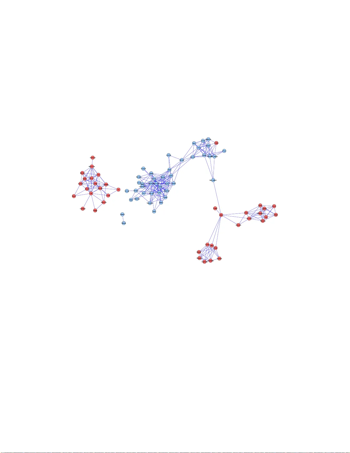
Model Selection Thr ough Sp arse Max Likelihood Estima tion Mo del Selection Through Sparse Maxim um Lik eliho o d Estimation for Multiv aria te G a ussian or Binary Data On ureena Banerjee onureena@eecs.berkeley.edu Lauren t El Ghaoui elghaoui@eec s.berkeley.edu EECS Dep artment University of California, Berkeley Berkeley, CA 94720 US A Alexandre d’Aspremon t aspremon@princeton.edu ORFE Dep artment Princ eton Un i versity Princ eton, NJ 08544 U SA Editor: Leslie P ack Kaelbling Abstract W e consider the problem of estimating the par ameters of a Gaussian or binary distr ib ution in such a wa y that the resulting undirec t ed g raphical mo del is spa rse. Our approach is to so lve a maximum lik eliho od pr o blem with an added ℓ 1 -norm p enalt y term. The problem as for m ulated is co n vex but the memory requir emen ts and complex it y of existing int erior point methods are prohibitiv e for problems with more than tens of no des. W e present t w o new algor ithms for solving problems with at least a thousand nodes in the Gaussian case. Our fir st algo rithm uses blo c k co ordinate descent, and can b e interpreted as r ecursiv e ℓ 1 -norm pena lized regr ession. O ur seco nd algo rithm, ba sed on Nesterov’s firs t order metho d, yields a c o mplexit y estimate with a better dependence on proble m size than existing interior po int metho ds. Using a log determinant relaxa t ion o f the lo g partition function (W ain wr igh t and Jo rdan [2006]), we sho w that these same algorithms can be used to solve an approximate sparse maximum likelihoo d problem for the binary cas e. W e tes t our a lgorithms on synthetic data, as well a s o n gene expressio n and senate voting records data. Keyw ords: Mo del Selection, Maxim um Likelihoo d Estimation, Con vex Optimization, Gaussian Graphica l Model, Binary Data 1 Banerjee, El Ghaoui, and d’Aspremont 1. In tr oduction Undirected graphical mo dels offer a wa y to describ e and explain the relationships among a set of v ariables, a cen tral elemen t of m ultiv ariate data analysis. Th e principle of parsimony dictates that w e should select the simplest graph i cal mod e l that adequately explains the data. In this pap er weconsider practical w a ys of implement ing the follo wing approac h to finding such a mo del: giv en a set of data, w e solv e a maxim um lik eliho o d pr o blem with an added ℓ 1 -norm p enalt y to mak e the resulting graph as sparse as p ossible. Man y authors h a v e studied a v ariety of related ideas. In th e Gaussian case, mo del selection in v olv es fin ding the pattern of zeros in the in v erse co v ariance matrix, since th ese zeros corresp ond to conditional ind ep endencies among the v ariables. T raditionally , a greedy forw ard-bac kw ard searc h al gorithm is used to determine the zero pattern [e.g., Laur i tzen, 1996]. Ho w ever, this is computationally infeasible for d a ta w ith ev en a mo derate num b er of v ariables. Li and Gui [2005] introd uce a gradient descent algorithm in whic h th e y account for the sparsit y of the in v ers e co v ariance matrix b y definin g a loss function that is the negativ e of the log likelihoo d function. Recen tly , Huang et al. [2005] considered p enalized maxim um lik eliho od estimation, and Dahl et al. [2006] prop osed a set of large scale metho ds for pr o blems where a sparsit y pattern for the inv erse co v ariance is giv en and one must estimate the nonzero elemen ts of the m a trix. Another wa y to estimate the graph i cal mo del is to find the set of n e igh b ors of eac h node in the graph b y regressing that v ariable aga inst th e r e maining v ariables. In this v ein, Dobra and W est [2004] employ a sto c hastic algorithm to manage tens of thousand s of v ari- ables. There has also b een a great deal of in terest in u sing ℓ 1 -norm p enalties in statistical applications. d’Aspr e mon t et al. [2004] apply an ℓ 1 norm p enalt y to s parse principle comp o- nen t analysis. Directly r e lated to our problem is the use of the Lasso of Tibshirani [1996] to obtain a v ery short list of neigh b ors for eac h n ode in the graph. Meinshausen and B ¨ uhlmann [2006] study this appr o ac h in detail, and sho w that th e resulting estimator is consistent, ev en for high-dimensional graphs. The problem formulati on for Gaussian d a ta, therefore, is simp le . The difficulty lies in its computation. Although the pr o blem is con v ex, it is non-smo oth and has an un b ounded constrain t set. As w e shall see, the resulting complexit y for existing in terior p oin t metho ds is O ( p 6 ), wher e p is the num b er of v ariables in the distribu tion. In add it ion, interior p oin t metho ds require that at eac h step w e compute and store a Hessian of size O ( p 2 ). The memory requirements and c omplexit y are thus prohib i tiv e for O ( p ) h igher than the te ns. Sp ecializ ed algorithms are n e eded to h a ndle larger problems. The remainder of the pap er is organized as follo ws. W e b egin by considering Gaussian data. I n Section 2 w e set u p the pr o blem, d e riv e its d u a l, d i scuss prop erties of the solution and how hea vily to w eigh t the ℓ 1 -norm p enalt y in our pr o blem. In Section 3 we present a pro v ably con v ergen t blo c k co ordinate descen t algorithm that can b e in terpreted as recursiv e ℓ 1 -norm p enaliz ed regression. In Sect ion ?? w e presen t a second, alternativ e algorithm based 2 Model Selection Through Sp arse Max L ikelihood Estima tion on Ne stero v’s recen t wo rk on non-smo oth optimization, and giv e a rigorous complexit y analysis with b etter dep endence on problem s i ze than interior p oin t metho ds. In Section ?? w e s h o w that the algorithms we dev elop ed for the Gaussian case can also b e used to solv e an app r o ximate sp a rse maximum lik eliho od problem for multiv ariate b i nary data, usin g a log determinan t r e laxation f o r th e log partition function giv en by W ainwrigh t and Jordan [2006]. In Section 6, we test our metho ds on synthet ic as w ell as gene expression and senate v oting records data. 2. Problem F orm ulation In this section w e set up the sp a rse maximum lik eliho od problem for Gaussian data, derive its du a l, and discu ss some of its prop erties. 2.1 Problem setup. Supp ose w e are giv en n samples ind e p enden tly dra w n from a p -v ariate Gaussian distribution: y (1) , . . . , y ( n ) ∼ N (Σ p , µ ), wh er e the co v ariance m atrix Σ is to b e estimated. L et S denote the second momen t matrix ab out the mean: S := 1 n n X k =1 ( y ( k ) − µ )( y ( k ) − µ ) T . Let ˆ Σ − 1 denote our estimate of the inv erse co v ariance matrix. Our estimato r tak es the form: ˆ Σ − 1 = arg ma x X ≻ 0 log det X − trace( S X ) − λ k X k 1 . (1) Here, k X k 1 denotes the su m of the absolute v alues of the elemen ts of the p ositiv e defin ite matrix X . The scalar paramet er λ control s the size of the p enalt y . Th e p enalt y term is a pro xy for the n um b er of nonzero elemen ts in X , and is often us e d – a lbiet with v ector, not matrix, v ariables – in regression tec hniques, s u c h as the Lasso. In the case wh er e S ≻ 0, the classical maxim um lik eliho o d estimate is r e co vered for λ = 0. Ho wev er, when the num b er of samples n is small compared to the num b er of v ariables p , the second moment matrix ma y n o t b e inv ertible. In s uc h cases, for λ > 0, our estimator p erforms some regularization so that o ur estimate ˆ Σ is alw a ys inv ertible, n o matter ho w small the r a tio of s amp le s to v ariables is. 3 Banerjee, El Ghaoui, and d’Aspremont Ev en in ca ses wh er e w e ha ve enough samples so that S ≻ 0, the in verse S − 1 ma y not b e sp a rse, even if there are man y cond itional ind e p endencies amo ng the v ariables in the distribution. By trading off maximalit y of the log likel iho od for sparsity , w e hop e to find a v ery s p a rse solution that s till ad equ a tely explains the data. A larger v alue of λ corresp onds to a sparser solution that fi t s the data less well . A smaller λ corresp onds to a solution that fits the data we ll but is less s parse. The c hoice of λ is therefore an imp ortan t issue that will b e examined in detail in S ection 2.3. 2.2 The dual problem and b ounds on the solution. W e can write (1 ) as max X ≻ 0 min k U k ∞ ≤ λ log det X + trace( X , S + U ) where k U k ∞ denotes the maxim um absolute v alue elemen t of the symmetric matrix U . This corresp onds to seeking an estimate with the m aximum w orst-case log lik eliho od , o ver a ll additiv e p erturbations of the second momen t matrix S . A similar robustness int erpretation can b e made f or a n um b er of estimation p roblems, such as su p port vec tor mac h in e s f o r classification. W e can obtain the d ual p roblem by exc hanging the max and the min . The resulting in n er problem in X can b e solv ed analytically b y setting the gradient of the ob jectiv e to zero and solving for X . The result is min k U k ∞ ≤ λ − log d e t( S + U ) − p where the prim al and du a l v ariables are related as: X = ( S + U ) − 1 . Not e that the log determinan t fu nct ion acts a log b a rrier, creating an implicit constrain t that S + U ≻ 0. T o write things neatly , let W = S + U . Then the du a l of our sparse m aximum lik eliho od problem is ˆ Σ := max { log det W : k W − S k ∞ ≤ λ } . (2) Observe that the d ual problem (1) estimates the co v ariance matrix wh il e the primal p r o blem estimates its inv erse. W e also observe that the diagonal elemen ts of the solution are Σ k k = S k k + λ for all k . The follo wing theorem sho ws that adding the ℓ 1 -norm p enalt y regularlizes the solution. Theorem 1 F or every λ > 0 , the optimal solution to (1) is unique, with b ounde d eigenval- ues: p λ ≥ k ˆ Σ − 1 k 2 ≥ ( k S k 2 + λp ) − 1 . Here, k A k 2 denotes the m a xim um eigenv alue of a symmetric matrix A . 4 Model Selection Through Sp arse Max L ikelihood Estima tion The dual p roblem (2) is sm ooth and con v ex. When p ( p + 1) / 2 is in the lo w h undreds, the problem can b e solv ed by existing soft w are that uses an inte rior p oin t metho d [e.g., V andenberghe et al., 199 8]. The complexit y to compu t e an ǫ -sub optimal solution using suc h s e cond-order metho ds, ho wev er, is O ( p 6 log(1 /ǫ )), making them infeasible when p is larger than th e tens. A relat ed problem, solv ed by Dahl et al. [200 6], is t o co mpute a maximum lik eliho od es- timate of the co v ariance matrix when the sparsit y structure of the inv erse is kno wn in adv ance. This is a ccomplished b y adding c onstrain ts to (1) of the form: X ij = 0 for all pairs ( i, j ) in some s pecified s e t. Our constrain t set is un b ounded as w e h o p e to unco v er the sp a rsit y structure automatically , starting with a dense s econd momen t matrix S . 2.3 Choice of p enalt y parameter. Consider the true, unknown graphical mo del for a give n distribution. This graph has p no des, and an edge b et wee n no des k and j is missin g if v ariables k and j are indep enden t conditional on the rest of the v ariables. F or a giv en no de k , let C k denote its connectivit y comp onen t: the set of all no des that are connected to no de k through some c h a in of edges. In particular, if no de j 6∈ C k , then v ariables j a nd k are indep endent . W e w ould lik e to c h oose the p enalt y parameter λ so that, for fi nite samp les, the probabilit y of error in estimating the graph ical mo del is controll ed. T o this en d, we can adapt the work of Meinshausen and B ¨ uhlmann [2006] as follo ws. Let ˆ C λ k denote our estimate of the connec- tivit y comp onen t of n ode k . In the con text of our optimizatio n pr o blem, this corr esp onds to the en tries of row k in ˆ Σ that are nonzero. Let α b e a give n level in [0 , 1]. Consid er the follo win g c hoice for the p enalt y parameter in (1): λ ( α ) := (max i>j ˆ σ i ˆ σ j ) t n − 2 ( α/ 2 p 2 ) q n − 2 + t 2 n − 2 ( α/ 2 p 2 ) (3) where t n − 2 ( α ) d e notes the (100 − α )% p oint of the Stu den t’s t-distribu t ion for n − 2 degrees of fr eedom, and ˆ σ i is the empirical v ariance of v ariable i . Then we can pr o v e the follo win g theorem: Theorem 2 Using λ ( α ) the p enalty p ar ameter in (1), for any fixe d level α , P ( ∃ k ∈ { 1 , . . . , p } : ˆ C λ k 6⊆ C k ) ≤ α. Observe that, for a fix ed prob lem size p , as the num b er of samples n incr eases to infi nit y , the p e nalt y parameter λ ( α ) decrea ses to zero. Thus, asymp totically w e reco v er the clas- 5 Banerjee, El Ghaoui, and d’Aspremont sical maximum like liho od estimate, S , whic h in turn conv erges in pr o babilit y t o the true co v ariance Σ. 3. Blo c k Co ordin ate Descen t Algorit hm In this section we pr esen t an algorithm for solving (2) that uses b lo c k co ordin ate descen t. 3.1 Algorithm description. W e b egin b y detail ing the al gorithm. F or a n y symmetric matrix A , let A \ j \ k denote the matrix p ro du ced by remo ving ro w k and column j . Let A j denote column j w ith the diagonal ele men t A j j remo v ed. T he plan is to optimize o ver one r o w and column of the v ariable matrix W at a time, and to rep eatedly sweep through all columns until we ac h iev e con vergence. Initialize: W (0) := S + λI F or k ≥ 0 1. F or j = 1 , . . . , p (a) Let W ( j − 1) denote the cur ren t iterate. Solve the quadratic pr ogram ˆ y := arg min y { y T ( W ( j − 1) \ j \ j ) − 1 y : k y − S j k ∞ ≤ λ } (4) (b) Up d ate rule: W ( j ) is W ( j − 1) with column/row W j replaced by ˆ y . 2. Let ˆ W (0) := W ( p ) . 3. After eac h sw eep thr ough all columns, c hec k the conv ergence condition. Conv ergence o ccurs wh en trace(( ˆ W (0) ) − 1 S ) − p + λ k ( ˆ W (0) ) − 1 k 1 ≤ ǫ. (5) 3.2 Con v e rgence and prop erty of solution. Using Sch u r complements, we can pr o ve con v ergence: Theorem 3 The blo ck c o or dinate desc ent algorithm describ e d ab ove c onver ges, acheiving an ǫ -su b optima l solution to (2). In p articular, the i ter ates pr o duc e d by the algorithm ar e strictly p ositive definite: e ach time we swe ep thr ough the c olumns, W ( j ) ≻ 0 for al l j . 6 Model Selection Through Sp arse Max L ikelihood Estima tion The pro of of Theorem 3 sheds so me in teresting ligh t on th e solution to problem (1). In particular, we can use this metho d to sh o w that th e solution has the follo wing prop ert y: Theorem 4 Fix any k ∈ { 1 , . . . , p } . If λ ≥ | S k j | for al l j 6 = k , th en c olumn and r ow k of the solution ˆ Σ to (2) ar e zer o, excluding the diagonal element. This means that, for a give n s econd momen t matrix S , if λ is c h osen su c h th at the condition in Theorem 4 is met for some column k , then the sparse maximum likel iho o d metho d esti- mates v ariable k to b e indep endent of all other v ariables in the distribu tion. In particular, Theorem 4 imp lies that if λ ≥ | S k j | for all k > j , then (1) estimates all v ariables in the distribution to b e pairwise indep endent. Using the work of Lu o and Tsen g [1992], it may b e p ossib le to sho w that the lo cal conv er- gence r ate of this metho d is at least linear. In practice w e ha v e found that a s m all n um b er of sweeps through all columns, indep endent of p roblem size p , is sufficient to ac hiev e co n- v ergence. F or a fixed num b er of K sweeps, the cost of the metho d is O ( K p 4 ), since eac h iteration costs O ( p 3 ). 3.3 In terpretation as recursiv e penalized regression. The du al of (4) is min x x T W ( j − 1) \ j \ j x − S T j x + λ k x k 1 . (6) Strong d ualit y obtains so that pr oblems (6) and (4) are equiv alen t. If w e let Q denote the square ro ot of W ( j − 1) \ j \ j , and b := 1 2 Q − 1 S j , then w e can wr ite (6) as min x k Qx − b k 2 2 + λ k x k 1 . (7) The pr oblem (7) is a p enalized least-squares p roblems, kn own as th e Lasso. If W ( j − 1) \ j \ j w ere the j -th pr incipal minor of the sample co v ariance S , then (7) w ould b e equiv alen t to a p enalized regression of v ariable j ag ainst all others. T h us, the appr oac h is reminiscen t of the appr oac h explored by Meinshau s en and B ¨ uhlmann [2006], bu t there are t wo differences. First, w e b egin w ith some regularization and, as a consequence, eac h p en alized regression problem has a u nique solution. Second, and more imp ortan tly , w e up date the problem data after eac h regression: except at the ve ry fir st up date, W ( j − 1) \ j \ j is n ev er a minor of S . In this sense, the coord inate descent metho d can b e in terpreted as a recurs ive Lasso. 7 Banerjee, El Ghaoui, and d’Aspremont 4. Nestero v’s First Order Metho d In this section we apply the recen t results d ue to Nesterov [2005] to obtain a first order algo- rithm for solving (1) with lo wer memory requ iremen ts and a rigorous complexit y estimate with a b etter dep endence on pr oblem size th an those offered by in terior p oin t metho ds. Our pur p ose is not to obtain another algorithm, as we ha v e found that the blo c k co ordin ate descen t is fairly efficien t; rather, w e seek to use Nestero v’s formalism to derive a r igorous complexit y estimate for the problem, imp r o v ed o v er that offered by in terior-p oin t metho ds. As we will see, Nestero v’s framewo rk allo ws us to obtain an algorithm that has a complexit y of O ( p 4 . 5 /ǫ ), where ǫ > 0 is the desired accuracy on the ob jectiv e of problem (1). This is in c on trast to the complexit y of interio r-p oint metho d s, O ( p 6 log(1 /ǫ )). Th us, Nest ero v’s metho d provides a muc h b etter dep endence on problem size and lo w er m emory r equiremen ts at the exp ense of a degraded dep end ence on accuracy . 4.1 Idea of Nesterov’s metho d. Nestero v’s method applies to a class of non-smooth, con ve x optimization problems of the form min x { f ( x ) : x ∈ Q 1 } (8) where the ob jectiv e fu nction can b e written as f ( x ) = ˆ f ( x ) + max u {h Ax, u i 2 : u ∈ Q 2 } . Here, Q 1 and Q 2 are b ounded, closed, con v ex sets, ˆ f ( x ) is d ifferen tiable (with a Lipsc hitz- con tinuous gradien t) and con v ex on Q 1 , and A is a linear op erator. The c h allenge is to write our problem in the appropriate form and choose asso ciated fu n ctions and parameters in suc h a wa y as to obtain the b est p ossible complexit y estimate, by applying general r esults obtained by Nesterov [2005]. Observe that w e ca n wr ite (1) in the form (8) if we imp ose b oun ds on the e igen v alues of the solution, X . T o this end , we let Q 1 := { x : aI  X  bI } Q 2 := { u : k u k ∞ ≤ λ } (9) where the constants a, b are giv en suc h that b > a > 0. By Theorem 1, we kn ow that suc h b oun d s alwa ys exist. W e also define ˆ f ( x ) := − log det x + h S, x i , and A := λI . T o Q 1 and Q 2 , w e asso ciate norm s and cont in uous, strongly con v ex fu nctions, called pro x- functions, d 1 ( x ) and d 2 ( u ). F or Q 1 w e c ho ose the F rob enius n orm, and a prox-function 8 Model Selection Through Sp arse Max L ikelihood Estima tion d 1 ( x ) = − log det x + log b . F or Q 2 , w e choose the F rob enius norm agai n, and a p r o x- function d 2 ( x ) = k u k 2 F / 2. The metho d applies a s m o othing tec hn ique to the non-smo oth prob lem (8), which replaces the ob jectiv e of th e original problem, f ( x ), by a p enalized function inv olving the p ro x- function d 2 ( u ): ˜ f ( x ) = ˆ f ( x ) + max u ∈ Q 2 {h Ax, u i − µd 2 ( u ) } . (10) The ab o v e fu nction tur n s out to b e a smo oth un iform appr oximati on to f ev erywhere. It is d ifferentiable, conv ex on Q 1 , and a has a Lipsc hitz-con tinuous gradien t, with a constan t L that can b e computed as detailed b elo w. A s p ecific gradien t scheme is then applied to this smo oth appro ximation, w ith con v ergence rate O ( L/ǫ ). 4.2 Algorithm and complexity estimate. T o detail the algo rithm and compute the complexit y , we m u st first calc ulate some pa- rameters corresp onding to our definitions a nd c h oices ab ov e. First, the strong con ve xit y parameter for d 1 ( x ) on Q 1 is σ 1 = 1 /b 2 , in the sense that ∇ 2 d 1 ( X )[ H, H ] = trace( X − 1 H X − 1 H ) ≥ b − 2 k H k 2 F for every symmetric H . F ur th ermore, the cen ter of th e set Q 1 is x 0 := arg min x ∈ Q 1 d 1 ( x ) = bI , and satisfies d 1 ( x 0 ) = 0. With our c hoice, we h a v e D 1 := max x ∈ Q 1 d 1 ( x ) = p log ( b/a ). Similarly , th e strong conv exit y parameter for d 2 ( u ) on Q 2 is σ 2 := 1, and w e hav e D 2 := m ax u ∈ Q 2 d 2 ( U ) = p 2 / 2 . With this c h oice, the cen ter of the s et Q 2 is u 0 := arg min u ∈ Q 2 d 2 ( u ) = 0. F or a desired accuracy ǫ , w e set the sm o othness parameter µ := ǫ/ 2 D 2 , and s et x 0 = bI . The algorithm p ro ceeds as follo w s: F or k ≥ 0 do 1. Compute ∇ ˜ f ( x k ) = − x − 1 + S + u ∗ ( x k ), wher e u ∗ ( x ) solv es (10 ). 2. Find y k = arg min y {h∇ ˜ f ( x k ) , y − x k i + 1 2 L ( ǫ ) k y − x k k 2 F : y ∈ Q 1 } . 3. Find z k = arg min x { L ( ǫ ) σ 1 d 1 ( X ) + P k i =0 i +1 2 h∇ ˜ f ( x i ) , x − x i i : x ∈ Q 1 } . 9 Banerjee, El Ghaoui, and d’Aspremont 4. Up d ate x k = 2 k +3 z k + k +1 k +3 y k . In our case, the Lipsc h itz constan t for the gradien t of our smo oth app ro ximation to the ob jectiv e fu nction is L ( ǫ ) := M + D 2 k A k 2 / (2 σ 2 ǫ ) where M := 1 /a 2 is the Lip sc hitz constan t for th e gradien t of ˜ f , and the norm k A k is induced by the F rob enius norm , and is equal to λ . The algorithm is guarante ed to pr o duce an ǫ -su b optimal solution after a n um b er of steps not exceeding N ( ǫ ) := 4 k A k r D 1 D 2 σ 1 σ 2 · 1 ǫ + q M D 1 σ 1 ǫ = ( κ p (log κ ) )(4 p 1 . 5 aλ/ √ 2 + √ ǫp ) /ǫ. (11) where κ = b/a is a b oun d on the condition num b er of the solution. No w we are ready to estimate the complexit y of the algorithm. F or Step 1, the gradien t of the smo oth a pproxima tion is c omputed in closed form b y taking the in verse of x . Step 2 essen tially amoun ts to pro jecting on Q 1 , and r equires that w e solv e an eigen v alue problem. The same is true for Step 3. In fact, eac h iteratio n costs O ( p 3 ). T he num b er of iterations necessary to ac hiev e an ob jectiv e with absolute accuracy less than ǫ is give n in (11 ) by N ( ǫ ) = O ( p 1 . 5 /ǫ ). Th us, if the condition num b er κ is fixed in adv ance, th e complexit y of the algorithm is O ( p 4 . 5 /ǫ ). 5. Binary V aria bles: Appro ximate Sparse Ma xim um Likelihoo d Estimation In this section, we consid er the problem of estimating a n undirected g raphical mo del fo r m ultiv ariate binary d ata. Recently , W ain wright et al. [2006] applied an ℓ 1 -norm p enalt y to the logistic regression problem to obtain a binary v ers ion of the h igh-dimensional consistency results of Meinshausen and B ¨ uhlmann [2006 ]. W e apply the log determinant r elaxation of W ain wrigh t and Jordan [2006] to form ulate an appro ximate sparse maxim um likel iho o d (ASML) problem for estimating the parameters in a m ultiv ariate binary distr ib ution. W e sho w that the r esu lting problem is the same as the Gaussian sparse maxim um lik eliho o d (SML) problem, and that we can therefore apply our previously-dev elop ed algorithms to sparse mo d el selection in a bin ary setting. 10 Model Selection Through Sp arse Max L ikelihood Estima tion Consider a distribu tion made up of p binary rand om v ariables. Usin g n data s amples, w e wish to estimate th e stru cture of the distribution. T he logistic mo d el of this d istr ibution is p ( x ; θ ) = exp { p X i =1 θ i x i + p − 1 X i =1 p X j = i +1 θ ij x i x j − A ( θ ) } (12) where A ( θ ) = log X x ∈X p exp { p X i =1 θ i x i + p − 1 X i =1 p X j = i +1 θ ij x i x j } (13) is the log partition fu nction. The sparse maxim um lik elihoo d problem in this case is to maximize (12) with an add ed ℓ 1 -norm p enalt y on terms θ k j . Sp ecifically , in the undirected graph ical mo del, an edge b et w een no des k and j is missing if θ k j = 0. A w ell-kno wn difficult y is that the lo g partition function has to o man y terms in its outer sum to compute. Ho w ev er, if we use the log determinan t relaxation for the log partition function d ev eloped by W ain wrigh t and Jordan [2006], w e can obtain an approxi mate sp arse maxim um lik eliho o d (ASML) estimate. W e s hall set up the problem in the next section. 5.1 Problem form ulation. Let’s b egin with some notation. Letting d := p ( p + 1) / 2, d efine the m ap R : R d → S p +1 as follo ws: R ( θ ) =      0 θ 1 θ 2 . . . θ p θ 1 0 θ 12 . . . θ 1 p . . . θ p θ 1 p θ 2 p . . . 0      Supp ose that our n samples are z (1 ) , . . . , z ( n ) ∈ {− 1 , +1 } p . Let ¯ z i and ¯ z ij denote sample mean and second moments. The sparse maximum likel iho o d pr oblem is ˆ θ exact := arg max θ 1 2 h R ( θ ) , R ( ¯ z ) i − A ( θ ) − λ k θ k 1 . (14) Finally d efine the constant v ector m = (1 , 4 3 , . . . , 4 3 ) ∈ R p +1 . W ainwrigh t and Jordan [2006] giv e an upp er b oun d on the log p artition function as the solution to th e follo wing v ariational problem: A ( θ ) ≤ max µ 1 2 log det( R ( µ ) + diag( m )) + h θ , µ i = 1 2 · max µ log det( R ( µ ) + diag( m )) + h R ( θ ) , R ( µ ) i . (15) 11 Banerjee, El Ghaoui, and d’Aspremont If we use the b ound (15) in our sparse m axim um lik eliho o d p roblem (14), w e won’t b e able to extract an optimizing argument ˆ θ . O ur first step, therefore, will b e to rewrite the b ound in a form that will allo w this. Lemma 5 We c an r ewrite the b ound (15) as A ( θ ) ≤ p 2 log( eπ 2 ) − 1 2 ( p + 1) − 1 2 · { max ν ν T m + log det( − ( R ( θ ) + diag ( ν ))) . (16) Using this v ersion of the b ound (15), we h a v e the follo wing th eorem. Theorem 6 Using the upp er b ound on the lo g p artition function given in (16), the appr ox- imate sp arse maximum likeliho o d pr oblem has the fol lowing solution: ˆ θ k = ¯ µ k ˆ θ k j = − ( ˆ Γ) − 1 k j (17) wher e the matrix ˆ Γ is the solution to the fol lowing pr oblem, r elate d to (2): ˆ Γ := arg max { log d et W : W k k = S k k + 1 3 , | W k j − S k j | ≤ λ } . (18) Here, S is defin ed as b efore: S = 1 n n X k =1 ( z ( k ) − ¯ µ )( z ( k ) − ¯ µ ) T where ¯ µ is the v ector of samp le means ¯ z i . In particular, this mea ns that w e can reu se the algorithms devel op ed in Sections 3 and ?? for prob lems with binary v ariables. The relaxation (15) is the simp lest one offered by W ain wrigh t and Jordan [2006]. The relaxation can b e tightened by adding linear constrain ts on the v ariable µ . 5.2 P e nalt y parameter c hoice for binary v ariables. F or the c hoice of the p enalt y p arameter λ , w e can derive a formula analogo us to (3). Consider the c h oice λ ( α ) bin := ( χ 2 ( α/ 2 p 2 , 1)) 1 2 (min i>j ˆ σ i ˆ σ j ) √ n (19) 12 Model Selection Through Sp arse Max L ikelihood Estima tion where χ 2 ( α, 1) is the (1 00 − α )% p oint of the c h i-square distribution for one d egree of freedom. Since our v ariables take on v alues in {− 1 , 1 } , the empirical v ariances are o f the form: ˆ σ 2 i = 1 − ¯ µ 2 i . Using (19), w e ha v e th e follo wing b inary version of Theorem 2: Theorem 7 With (19) chosen a s the p enalty p ar ameter in the appr oximate sp arse maxi- mum likeliho o d pr oblem, for a fixe d level α , P ( ∃ k ∈ { 1 , . . . , p } : ˆ C λ k 6⊆ C k ) ≤ α. 6. Numerical Results In th is section w e p r esen t the resu lts of some numerical exp er im ents, b oth on syn thetic and real data. 6.1 Syn thetic exp eriments. Synt hetic exp eriments require that w e generate un derlying sparse inv erse co v ariance matri- ces. T o this end, w e first rand omly choose a diagonal matrix w ith p ositiv e d iagonal en tries. A giv en num b er of nonzeros are in serted in th e matrix at ran d om lo cations sym metrically . P ositiv e definiteness is ensur ed by adding a m ultiple of the iden tit y to the matrix if needed. The multiple is c hosen to b e only as large as necessary for inv ersion with n o errors . 6.1.1 Sp arsity and thresh olding. A v ery simple app roac h to obtaining a sparse estimate of the inv erse co v ariance matrix w ould b e to apply a thresh old to the inv erse empirical co v ariance matrix, S − 1 . Ho w ev er , ev en when S is easily in v ertib le, it can b e difficult to select a thr eshold lev el. W e solv ed a syn thetic problem of size p = 100 where the true concen tration matrix d ensit y was set to δ = 0 . 1. Dra wing n = 200 samples, we plot in Figure (1) the sorted absolute v alue elemen ts of S − 1 on the left and ˆ Σ − 1 on the righ t. It is clearly easier to choose a threshold lev el for the S ML estimate. Applying a thr esh old to either S − 1 or ˆ Σ − 1 w ould decrease the log lik eliho o d of the estimate by an unkn own amoun t. W e only observ e th at to preserve p ositiv e d efiniteness, the threshold lev el t must satisfy the b oun d t ≤ min k v k 1 ≤ 1 v T S − 1 v . 13 Banerjee, El Ghaoui, and d’Aspremont 0 2000 4000 6000 8000 10000 0 2 4 6 8 10 (A) 0 2000 4000 6000 8000 10000 0 2 4 6 8 10 (B) Figure 1: S orted ab s olute v alue of elemen ts of (A) S − 1 and (B) ˆ Σ − 1 . T he s olution ˆ Σ − 1 to (1) is un-thresholded. 6.1.2 Recovering s tructure. W e b egin with a small exp eriment to test the a bilit y of th e metho d to reco v er the sparse structure of an un derlying co v ariance matrix. Figure 2 (A) sho ws a sparse inv erse co v ariance matrix of size p = 30. Figure 2 (B) displa ys a c orresp ond ing S − 1 , u s ing n = 60 sa mples. Figure 2 (C) displa ys the solution to (1) f or λ = 0 . 1. The v alue of the p enalt y p arameter here is c hosen arbitrarily , and the solution is not t hresholded. Neverthele ss, w e can still pic k out features that were present in the tru e underlyin g in v erse co v ariance matrix. A 10 20 30 5 10 15 20 25 30 B 10 20 30 5 10 15 20 25 30 C 10 20 30 5 10 15 20 25 30 Figure 2: R eco v ering th e sparsit y pattern. W e plot (A) the original inv erse co v ariance matrix Σ − 1 , (B) the noisy sample in v erse S − 1 , and (C) the solution to pr oblem (1) for λ = 0 . 1. Using the same underlying in v erse co v ariance matrix, w e rep eat th e exp eriment using smaller sample sizes. W e solve (1 ) for n = 30 and n = 20 using the same arbitrarily c h osen p enalt y parameter v alue λ = 0 . 1, and displa y the sol utions in Figure (3). As ex- p ected, our abilit y to pic k out features of the true inv erse co v ariance matrix d iminishes with the num b er of samples. This is an added r eason to c ho ose a larger v alue of λ wh en w e ha v e few er samples, as in (3 ). 14 Model Selection Through Sp arse Max L ikelihood Estima tion A 10 20 30 5 10 15 20 25 30 B 10 20 30 5 10 15 20 25 30 C 10 20 30 5 10 15 20 25 30 Figure 3: R eco v ering the sp arsit y p attern for small sample size. W e p lot (A) the original in v erse cov ariance matrix Σ − 1 , (B ) the solution to problem (1) for n = 30 and (C) the solution for n = 20. A p enalt y parameter of λ = 0 . 1 is used for (B) and (C). 0 0.1 0.2 0.3 0.4 0.5 0.6 0.7 −0.4 −0.2 0 0.2 0.4 0.6 0.8 1 P S f r a g r e p l a c e m e n t s ˆ Σ − 1 ij λ 0 0.05 0.1 0.15 0.2 0.25 0.3 0.35 0.4 0.45 0.5 −0.7 −0.6 −0.5 −0.4 −0.3 −0.2 −0.1 0 0.1 0.2 0.3 P S f r a g r e p l a c e m e n t s ˆ Σ − 1 i j λ λ ˆ Σ − 1 ij Figure 4: Path f ollo wing: elemen ts of solution to (1) as λ increases. Red lines corresp ond to elemen ts that are zero in the true inv erse cov ariance matrix; blue lines corresp ond to tru e nonzeros. V ertical lines mark a r ange of λ v alues us ing which w e reco v er the sp arsit y pattern exactly . 6.1.3 P a th following ex periments . Figure (4) shows t wo path follo w in g examples. W e solve t w o r andomly generated pr oblems of size p = 5 and n = 100 samples. T he red lines corresp ond to elemen ts of the solution that are zero in the tr ue underlying in v erse co v ariance matrix. The blu e lines corresp ond to true n onzeros. The v ertical lines mark r anges of λ for whic h w e reco v er the correct sparsit y pattern exactly . Note that, by Theorem 4, for λ v alues greater than those sh o w n, the solution will b e diagonal. 15 Banerjee, El Ghaoui, and d’Aspremont −0.5 0 0.5 1 0 1 2 3 4 5 6 7 P S f r a g r e p l a c e m e n t s Error (in %) log( λ/σ ) Figure 5: R eco v ering sp arsit y p attern in a matrix with add ed un if orm noise of size σ = 0 . 1. W e plot the a verage p ercen tage or m isclassified entries as a function of log ( λ/σ ). On a related note, w e obs erv e that (1) also works well in r eco vering the sparsity pattern of a matrix mask ed by noise. The follo wing exp eriment illustrates this observ ation. W e generate a sp arse in v erse co v ariance matrix of size p = 50 as describ ed ab o v e. Th en, instead of u sing an empirical co v ariance S as input to (1), we u se S = (Σ − 1 + V ) − 1 , wh ere V is a r andomly generated u niform noise of size σ = 0 . 1. W e th en solv e (1) f or v arious v alues of the p enalt y parameter λ . In figure 5, for a eac h of v alue of λ sh o wn, w e randomly selected 10 s ample co v ariance ma- trices S of size p = 50 and computed the n um b er of misclassified zeros and nonzero elemen ts in t he solution to (1). W e plot the av erage p ercenta ge of error s (n um b er of misclassified zeros plus misclassified nonzeros d ivided by p 2 ), as w ell as error bars corresp onding to one standard deviation. As sh o w n, the err or r ate is nearly zero on av erage w h en the p enalt y is set to equ al the n oise lev el σ . 6.1.4 CPU times ve rsus problem size. F or a sense of the practical p erformance of the Nestero v metho d and the blo ck co ordinate descen t metho d , we randomly selected 10 sample co v ariance matrices S for problem s izes p ranging fr om 400 to 1000.In eac h case, the n umber of samples n wa s chosen to b e ab out a third of p . In figur e 6 w e plot the av erage CPU time to ac hiev e a d ualit y gap of ǫ = 1. CPU times were computed using an AMD Athlo n 64 2.20Ghz pro cessor with 1.96GB of RAM. 16 Model Selection Through Sp arse Max L ikelihood Estima tion 400 500 600 700 800 900 1000 0 1000 2000 3000 4000 5000 6000 7000 8000 9000 Problem size p Average CPU times in seconds Figure 6: Average CPU times vs. prob lem s ize us ing blo c k co ord inate d escen t. W e plot the a verage CPU time (in seconds) to reac h a gap of ǫ = 0 . 1 v ersus problem size p . As sho wn, we are typicall y able to solv e a problem of size p = 1000 in ab out tw o and half hours. 6.1.5 Performance a s a binar y classifier. In th is section we numerically examine the abilit y of the sparse maxim um likel iho o d (SML) metho d to correctly classify elemen ts of the in v erse cov ariance matrix as zero or nonzero. F or comparision, w e will use th e Lasso estimate of Meinshausen and B ¨ uhlmann [200 6], whic h has b een sh o wn to p erform extremely w ell. The Lasso regresses eac h v ariable a gainst a ll others one at a time. Up on obtaining a solution θ ( k ) for eac h v ariable k , one can estimate sparsit y in one of tw o w ays: either b y declaring an elemen t ˆ Σ ij nonzero if b oth θ ( k ) i 6 = 0 and θ ( k ) j 6 = 0 (Lasso-AND ) or, less conserv ativ ely , if either o f those quan tities is nonzero (Lasso-OR). As noted previously , Meinshausen and B ¨ u h lmann [2006] ha v e also d eriv ed a formula for c h o osing their p enalt y parameter. Both the SML and Lasso p enalt y paramet er form ulas dep end on a chosen lev el α , which is a b ound on the same error probabilit y for eac h metho d . F or these exp er im ents, w e set α = 0 . 05. In the follo wing experiments, w e fi xed the problem size p at 30 and generated sparse un- derlying inv ers e cov ariance matrices as d escrib ed ab ov e. W e v aried the num b er of samples n from 10 to 310. F or eac h v alue of n shown, w e ran 30 trials in whic h we estimated the sparsit y p attern of the inv erse co v ariance matrix using th e S ML, Lasso-OR, and Lasso-AND 17 Banerjee, El Ghaoui, and d’Aspremont 1 2 3 4 5 6 7 8 9 10 11 0.2 0.3 0.4 0.5 0.6 0.7 0.8 0.9 1 Positive predictive value Ratio of samples to variables: n/p SML LASSO−V LASSO−& 1 2 3 4 5 6 7 8 9 10 11 0 0.05 0.1 0.15 0.2 0.25 0.3 0.35 Power Ratio of samples to variables: n/p SML LASSO−V LASSO−& 1 2 3 4 5 6 7 8 9 10 11 0 0.005 0.01 0.015 0.02 0.025 0.03 0.035 0.04 0.045 0.05 Density of solution Ratio of samples to variables: n/p SML LASSO−V LASSO−& True Figure 7: C lassifying zeros and nonzeros for a true density of δ = 0 . 05. W e plot the p ositiv e predictiv e v alue, the p ow er, and the estimated densit y u sing S ML, Lasso-OR and Lasso-AND. metho ds. W e th en recorded the a v erage num b er of n onzeros estimated b y e ac h metho d, and the av erage num b er of entries correctly iden tified as n onzero (true p ositiv es). W e sho w t w o sets of plots. Figure (7) corresp ond s to exp eriments where the true density w as set to b e lo w , δ = 0 . 05. W e plot the p ow er (prop ortion of correctly id en tified nonzeros), p ositiv e predictiv e v alue (prop ortion of estimated nonzeros that are correct), and the den s it y estimated b y eac h metho d. Figure (8) corresp onds to exp erimen ts wh ere the true densit y w as set to b e high, δ = 0 . 40, an d we p lot the same three quantiti es. 18 Model Selection Through Sp arse Max L ikelihood Estima tion 0 1 2 3 4 5 6 7 8 9 10 11 0.5 0.55 0.6 0.65 0.7 0.75 0.8 0.85 0.9 0.95 1 Positive predictive value Ratio of samples to variables: n/p SML LASSO−V LASSO−& 0 1 2 3 4 5 6 7 8 9 10 11 0 0.02 0.04 0.06 0.08 0.1 0.12 0.14 Power Ratio of samples to variables: n/p SML LASSO−V LASSO−& 0 1 2 3 4 5 6 7 8 9 10 11 −0.05 0 0.05 0.1 0.15 0.2 0.25 0.3 0.35 0.4 0.45 Density of solution Ratio of samples to variables: n/p SML LASSO−V LASSO−& True Figure 8: C lassifying zeros and nonzeros for a true density of δ = 0 . 40. W e plot the p ositiv e predictiv e v alue, the p ow er, and the estimated densit y u sing S ML, Lasso-OR and Lasso-AND. Meinshausen and B ¨ uh lmann [2006] rep ort that, asymptotically , Lasso-AND and Lasso-OR yield the same estimate of the sparsit y pattern of the inv erse co v ariance m atrix. At a fin ite n um b er of samp les, the S ML metho d seems to fall in in b etw een the t w o metho ds in terms of p o w er, p ositiv e predictiv e v alue, and the density of the estimate. It typica lly offers, on a verage , the lo w est total num b er of errors, tied with either Lasso-AND or Lasso-OR. Among the tw o Lasso metho d s , it would seem that if the true densit y is very lo w, it is sligh tly b etter to u se the more conserv ativ e Lasso-AND. If the densit y is higher, it m ay b e b etter to use Lasso-OR. Wh en the true densit y is un kno wn, we can ac hieve an accuracy comparable to 19 Banerjee, El Ghaoui, and d’Aspremont the b etter choice among the Lasso metho ds by computing the SML estimate. Figure (9) sho ws one example of sp ars it y pattern reco v ery w hen the tr ue density is lo w. A B C D Figure 9: C omparing sparsit y p attern reco v er y to the Lasso. (A) true co v ariance (B) L asso- OR (C) Lasso-AND (D) SML. The Lasso and SML metho d s hav e a comparable compu tational complexit y . Ho wev er, unlik e the Lasso, the SML metho d is not p arallelizable. P aralleliz ation w ould render the Lasso a more computationally attractiv e choi ce, since eac h v ariable can regressed against all other separately , at an individual cost of O ( p 3 ). In exchange, SML can offer a more accurate estimate of the sparsit y pattern, as w ell a s a w ell-conditioned estimate of the co v ariance matrix itself. 6.2 Gene expression and U.S. Se nate v oting records data. W e tested our algorithms on three s ets o f data: tw o ge ne expression data sets, as w ell as US Senate vot ing records. In this section w e br iefly explore the resulting graph ical mo dels. 20 Model Selection Through Sp arse Max L ikelihood Estima tion 6.2.1 Rosett a Inpha rma tics comp endium. W e applied our algorithms to the Roset ta Inpharm atics C omp end iu m of gene expression profiles describ ed by Hughes et al. [2000]. The 300 exp er im ent comp endiu m con tains n = 253 samples with p = 6136 v ariables. With a view to w ards obtaining a v ery sparse graph, w e replaced α/ 2 p 2 in (3) by α , and set α = 0 . 05. T he resu lting p enalt y paramete r is λ = 0 . 0313. This is a large p enalt y for this data set, and by applying Theorem 4 w e find that all b u t 270 of the v ariables are estimated to b e indep endent from all the rest, clearly a v ery conserv ativ e estimate. Figure (10) d ispla ys the r esulting graph . Figure 10: App lication to Hu ghes comp end iu m. T h e ab ov e graph r esults f r om solving (1) for th is data set with a p enalty parameter of λ = 0 . 0313 . Figure (11) closes in on a region of Figure (10), a cl uster of genes that is un connected to the remaining genes in this estimate. Acc ording to Gene Ontolo gy [see Consortium, 2000], these genes are asso ciated with iron h omeostasis. The probabilit y that a gene h as b een false included in this cluster is at most 0 . 05. As a second example, in Figure (12), we sh o w a su b graph of genes asso ciated w ith cellular mem brane fusion. All thr ee graphs were rendered using Cytoscap e. 21 Banerjee, El Ghaoui, and d’Aspremont Figure 11: App lication to Hughes dataset (closeup of Figur e (10). These genes are asso ci- ated w ith iron h omeostasis. Figure 12: App lication to Hughes dataset (subgrap h of Figure (10). T h ese genes are asso- ciated with cellular mem brane fusion. 22 Model Selection Through Sp arse Max L ikelihood Estima tion T able 1: Pred ictor genes f or LDL receptor. Accession Gene BF553500 Cbp/p300-intera cting transactiv a tor BF387347 EST BF405996 calcium ch annel, vol t age dependent NM 017158 cytochrome P450, 2c39 K03249 enoyl-CoA, hydra t ase/3-hydro x y a cyl Co A dehydrog. BE100965 EST AI411979 Carnitine O-acetyl transferase AI410548 3-hydro xy isobutyr yl-Co A hydrolase NM 017288 sodium channel, vol t age-ga ted Y00102 estr ogen receptor 1 NM 0 13200 carnitine p almitoyl transferase 1b 6.2.2 Iconix microarra y d a t a. Next we analyzed a s u bset of a 10 , 000 gene microarra y dataset from 160 drug treated rat liv er s Natsoulis et al. [2005]. In this study , r ats were treated with a v ariet y of fi brate, statin, or estrogen receptor agonist comp oun ds. T aking th e 500 genes w ith the highest v ariance, we once again replaced α/ 2 p 2 in (3) by α , and set α = 0 . 05. The resulting p enalty p arameter is λ = 0 . 0853 . By applying Theorem 4 we fin d that all bu t 339 of the v ariables are estimated to b e inde- p end en t from the rest. This estimate is less conserv ativ e than that obtained in the Hughes case since th e ratio of samples to v ariables is 160 to 500 in s tead of 253 to 6136. The first order neig h b ors of any no de in a Ga ussian graphical model form the set of pre- dictors for that v ariable. In the estimated obtained by solving (1), w e f ou n d that LDL receptor had one of the largest num b er of fi r st-order neigh b ors in th e Gaussian graphical mo del. T he LDL receptor is b eliev ed to b e one of the k ey med iators o f the effect of b oth statins and estrogenic comp ound s on L DL c holesterol. T able 1 lists s ome of the fi rst order neigh b ors of LDL receptor. It is p erhaps not su rprising that several of these genes are directly in v olve d in either lipid or steroid metab olism (K0324 9, AI4119 79, AI410548 , NM 01320 0, Y0010 2). Other genes suc h as Cbp/p300 are kn o wn to b e global transcriptional r egulators. Finally , some are un- annotated E S Ts. Their connection to th e LDL receptor in this analysis ma y provide clues to their function. 23 Banerjee, El Ghaoui, and d’Aspremont 6.2.3 Sena te voting re cords d a t a. W e conclud e our numerical exp erimen ts by testing our approximat e sparse maxim um like li- ho o d estimation metho d on b inary data. The d ata s et consists of US senate v oting records data f rom th e 109th congress (2004 - 2006). There are one hundred v ariables, corresp ond- ing to 100 s en ators. Eac h of the 542 samples is bill that wa s put to a v ote. Th e v otes are recorded as -1 for n o and 1 for yes. There a re ma n y m issing v alues in this d ataset, corresp onding to missed v otes. S ince our analysis dep end s on data v alues tak en solely f rom {− 1 , 1 } , it w as necessary to impu te v alues to these. F or this exp erimen t, w e replaced all missing v otes with no es (-1). W e c hose the p enalt y parameter λ ( α ) ac cording to (19), using a signifi cance lev el of α = 0 . 05. Figure (13) sh o ws the resulting graphical mo d el, r endered using Cytoscap e. Red no des corresp ond to Repub lican senators, and blue no des corresp ond to Demo cratic senators. W e can mak e some tent ativ e observ ations by browsing the net w ork of senators. As neigh b ors most Demo crats ha v e only other Demo crats and Rep ublicans ha v e only other Repub licans. Senator Ch afee (R, RI) h as only demo crats as h is neighbors, an observ ation that s upp orts media statemen ts made by and ab out Ch afee du ring those years. S enator Allen (R, V A) unites t wo otherw ise separate groups of Repu blicans and also pro vides a co nnection to the large clus ter of Demo crats through Ben Nelson (D, NE). S enator Lieb erman (D, CT) is connected to other Demo crats only through Kerr y (D, MA), his run ning mate in th e 2004 p resident ial election. Th ese observ ations also matc h media statemen ts made b y b oth pund its and p oliticians. Thus, although we obtained this graphical mo d el via a relaxation of th e log partition function, the resulting p icture is largely supp orted by con v en tional wisdom. Figure (14) sho ws a subgraph consisting of n eigh b ors of degree thr ee or lo w er of Senator Allen. Ac kno wledgmen ts W e are indebted to Georges Natsoulis for his interpretatio n of the Iconix dataset analysis and for gathering the senate v oting records. W e also thank Martin W ain wright, Bin Y u, P eter Bartlett, and Mic hael J ordan for man y enligh tening con versations. References D. Bertsek as. Nonline ar Pr o gr amming . A thena Scien tific, 1998. Gene On tology C onsortium. Gene on tology: to ol for the unifi cation of biology . N atur e Genet. , 25:25–29, 2000. 24 Model Selection Through Sp arse Max L ikelihood Estima tion Figure 13: US Senate, 109th Congress (2004 -2006) . The graph d ispla ys th e solution to (14) obtained using the log determinan t relaxation to the log partition fun ction of W ain wr igh t and Jordan [200 6]. Demo cratic senators are colored blue and Republican senators are colored red. 25 Banerjee, El Ghaoui, and d’Aspremont Figure 14: US Senate, 109th Congress. Neigh b ors of Senator Allen (degree th ree or low er). J. Dahl, V. Ro yc h o w dhury , and L. V andenb erghe. Co v ariance selection for non-c hordal graphs via c hordal embedd ing. Submitte d to Optimization Metho ds and Softwar e , 2006. Alexandre d’Aspremont, Laur en t El Gh aoui, M.I. Jord an, and G. R. G. Lanc kriet. A direct form ulation for sparse PC A usin g semidefin ite programming. A dvanc es i n Neu r al Information Pr o c essing Systems , 17, 2004. A. Dobra and M. W est. Ba y esian cov ariance selecti on. Working p ap er, ISDS, Duke Uni- versity , 2004. J. Z . Huang, N. Liu, and M. P ourahmadi. Cov ariance selection and estimattion via p enalized normal lik eliho o d. W harton Pr eprint , 2005. T. R . Hughes, M. J. Marton, A. R. Jones, C. J. Rob erts, R. Stoughto n, C. D. Armour, H. A. Bennett, E. Coffey , H. Dai, Y. D. He, M. J. Kid d, A. M. King, M. R. Mey er, D. Slade, P . Y. Lum, S. B. Stepanian ts, D. D. Sho emaker, D. Gac hotte, K. Chakraburtty , J. Simon, M. Bard, and S. H. F riend. F unctional disco v ery via a comp endiu m of expression p rofiles. Cel l , 102(1):10 9–126 , 20 00. S. Lauritzen. Gr aphic al Mo dels . Spr inger V erlag, 1996. H. Li and J. Gui. Gradient directed r egularization for sparse gaussian concen tration graphs, with applications to inf erence of genetic n etw orks. Unive rsity of Pennsylvania T e chnic al R ep ort , 2005. Z. Q . Lu o and P . Tseng. On the con v ergence of the co ordin ate d escen t metho d for con v ex differen tiable minimizat ion. Journal of Optimization The ory and Applic ations , 72(1): 7–35, 1992. 26 Model Selection Through Sp arse Max L ikelihood Estima tion N. Meinshausen and P . B ¨ uhlmann . High dimensional graphs and v ariable selection with the lasso. Annals of statistics , 34:1436–1 462, 2006. G. Natsoulis, L. El Ghaoui, G. Lanc kriet, A. T olley , F. Lero y , S. Du n lea, B. Eynon, C. Pe ar- son, S. T ugendreich, and K. Jarnagin. Classification of a large microarray data set: al- gorithm comparison and analysis of drug signatures. Genome R ese ar ch , 15:724 –736, 2005. Y. Nestero v. Smo oth minimization of non-smo oth f u nctions. M ath. Pr o g. , 103(1):127 –152, 2005. R. Tibshirani. Regression shr ink age and select ion via the lasso. Journal of the Royal statistic al so ciety, series B , 58(267-2 88), 1996 . Liev en V andenb erghe, Stephen Bo yd, and Shao-P o W u. Determinan t maximiza tion with linear matrix inequalit y constraints. SIAM Journal on Matrix Analysis and Applic ations , 19(4): 499 – 533, 1998. M. W a in wrigh t and M. Jordan . Log-determinant r elaxation for appr o x im ate inference in discrete marko v random fields . IEEE T r ansactions on Signal Pr o c essing , 2006. M. J. W ainwrigh t, P . Ra viku mar, and J . D. Laffert y . High-dimensional graph ical mo del selection using ℓ 1 -regularized logistic r egression. Pr o c e e dings of A dvanc es in Neur al In- formation Pr o c essing Systems , 2006. App endix A. Pro of of solution properties and blo c k co ordinate descen t con v ergence In this section, w e giv e short proofs of the tw o theorems o n prop erties of the solution to (1), as well as the con v er gence of the b lo c k co ordin ate descen t metho d . Pro of of Theorem 1: Since ˆ Σ satisfies ˆ Σ = S + ˆ U , where k U k ∞ ≤ λ , we ha v e: k ˆ Σ k 2 = k S + ˆ U k 2 ≤ k S k 2 + k U k 2 ≤ k S k 2 + k U k ∞ ≤ k S k 2 + λp whic h yields the lo w er b ound on k ˆ Σ − 1 k 2 . Lik ewise, w e can sho w that k ˆ Σ − 1 k 2 is b ound ed ab o v e. A t the optim um, the primal du al gap is zero: − log d et ˆ Σ − 1 + trace( S ˆ Σ − 1 ) + λ k ˆ Σ − 1 k 1 − log det ˆ Σ − p = trace( S ˆ Σ − 1 ) + λ k ˆ Σ − 1 k 1 − p = 0 27 Banerjee, El Ghaoui, and d’Aspremont W e therefore ha v e k ˆ Σ − 1 k 2 ≤ k ˆ Σ − 1 k F ≤ k ˆ Σ − 1 k 1 = p/λ − trace( S ˆ Σ − 1 ) /λ ≤ p/λ where the last inequality f ollo ws from trace( S ˆ Σ − 1 ) ≥ 0, since S  0 and ˆ Σ − 1 ≻ 0. Next we p ro v e the con v ergence of blo c k co ordin ate descent : Pro of of Theorem 3: T o s ee that optimizing ov er one ro w and column of W in (2) yields the qu adratic program (4), let all b ut the last row and column of W b e fi xed. Since w e know the diagonal en tries of the s olution, we can fix th e remaining diagonal en try as wel l: W =  W \ p \ p w p w T p W pp  Then, us ing Sc h ur complemen ts, w e hav e that det W = det W \ p \ p · ( W pp − w T p ( W \ p \ p ) − 1 w p ) whic h giv es rise to (4). By general results on blo c k co ordinate descent algorithms [e.g., Bertsek as, 1998], th e algo- rithms con v erges if and only if (4) has a uniqu e solution at eac h iteratio n. Thus it suffices to sho w th at, at ev er y swee p, W ( j ) ≻ 0 for all columns j . Prior to the first sweep, the in itial v alue of the v ariable is p ositiv e definite: W (0) ≻ 0 since W (0) := S + λI , and w e ha v e S  0 and λ > 0 by assump tion. No w supp ose that W ( j ) ≻ 0. T h is implies that th e follo win g Sch ur complemen t is p ositiv e: w j j − W T j ( W ( j ) \ j \ j ) − 1 W j > 0 By the up date rule we hav e that the c orresp ond ing S c hur complement for W ( j + 1) is ev en greater: w j j − W T j ( W ( j + 1) \ j \ j ) − 1 W j > w j j − W T j ( W ( j ) \ j \ j ) − 1 W j > 0 so that W ( j + 1) ≻ 0. Finally , w e apply T heorem 3 to prov e th e second prop erty of th e solution. Pro of of Theorem 4: 28 Model Selection Through Sp arse Max L ikelihood Estima tion Supp ose that column j of the second momen t matrix satisfies | S ij | ≤ λ for all i 6 = j . Th is means th at the zero v ector is in the co nstrain t set of (4) for that column. E ac h time we return to column j , the ob jectiv e fu nction will b e different, but alw a ys of the form y T Ay for A ≻ 0. S ince the constrain t set will not c hange, the solution for column j w ill alw a ys b e zero. By T heorem 3 , the blo c k co ordinate descen t algorithm con v erges to a solution, and so therefore th e solution m ust ha v e ˆ Σ j = 0. App endix B. Pro of of error bounds. Next we shall sho w that the p enalty p arameter c hoice give n in (3) yields the error pr ob ab ility b oun d of T heorem 2. The pro of is nearly identica l to that of [Meinshausen and B ¨ uh lmann, 2006,Theorem 3]. T he differences stem from a differen t ob jectiv e function, and the fact that our v ariable is a matrix of size p rather than a vec tor of size p . Our p r o of is only an adaptation of their p ro of to our problem. B.1 Preliminaries Before we b egin, consider problem (1), for a matrix S of an y size: ˆ X = arg min − log det X + trace( S X ) + λ k X k 1 where we hav e dr op p ed the constrain t X ≻ 0 since it is implicit, due to th e log determinant function. Since the problem is unconstrained, the solution ˆ X must corresp ond to setting the su bgradien t of the ob jectiv e to zero: S ij − X − 1 ij = − λ f or X ij > 0 S ij − X − 1 ij = λ for X ij < 0 | S ij − X − 1 ij | ≤ λ for X ij = 0 (20) Recall that b y Theorem 1 , the s olution is u nique for λ p ositiv e. B.2 Pro of of error b ound for Gaussian data. No w we are ready to prov e T heorem 2. Pro of of Theorem 2: Sort columns of the cov ariance matrix so that v ariables in the same connectivit y comp onent are group ed together. The correct zero p attern for the co v ariance matrix is then blo c k diagonal. Define Σ correct := blk diag( C 1 , . . . , C ℓ ) (21) 29 Banerjee, El Ghaoui, and d’Aspremont The inv erse (Σ correct ) − 1 m ust also b e blo c k d iagonal, with p ossib le additional zeros ins ide the blo c ks. If w e constrain the solution to (1) to ha ve th is stru cture, then b y the form of the ob jectiv e, w e c an optimize o v er eac h blo c k separately . F or eac h bloc k, th e sol ution is c h aracterized by (20). No w, sup p ose that λ > max i ∈ N ,j ∈ N \ C i | S ij − Σ correct ij | (22) Then, b y the subgradien t c haracterizatio n of the solution noted ab o ve, and the fact that the solution is u nique for λ > 0, it must b e the case that ˆ Σ = Σ correct . By the definition of Σ correct , this implies that, for ˆ Σ, we h av e ˆ C k = C k for all k ∈ N . T aking th e cont rap ositiv e of this statemen t, we can wr ite: P ( ∃ k ∈ N : ˆ C k 6⊆ C k ) ≤ P (max i ∈ N ,j ∈ N \ C i | S ij − Σ correct ij | ≥ λ ) ≤ p 2 ( n ) · max i ∈ N ,j ∈ N \ C i P ( | S ij − Σ correct ij | ≥ λ ) = p 2 ( n ) · max i ∈ N ,j ∈ N \ C i P ( | S ij | ≥ λ ) (23) The equalit y at the end f ollo ws since, by d efinition, Σ correct ij = 0 for j ∈ N \ C i . It remains to b ound P ( | S ij | ≥ λ ). The statemen t | S k j | ≥ λ can b e written as: | R k j | (1 − R 2 k j ) − 1 2 ≥ λ ( s k k s j j − λ 2 ) − 1 2 where R k j is the correlation b et w een v ariables k and j , since | R k j | (1 − R 2 k j ) − 1 2 = | S k j | ( S k k S j j − S 2 k j ) − 1 2 F urthermore, the condition j ∈ N \ C k is equiv alen t to sa ying that v ariables k and j are indep en den t: Σ k j = 0. Cond itional on this, the statistic R k j (1 − R 2 k j ) − 1 2 ( n − 2) 1 2 has a S tudent’s t-distribution for n − 2 degrees of freedom. Ther efore, f or all j ∈ N \ C k , P ( | S k j | ≥ λ | S k k = s k k , S j j = s j j ) = 2 P ( T n − 2 ≥ λ ( s k k s j j − λ 2 ) − 1 2 ( n − 2) 1 2 | S k k = s k k , S j j = s j j ) ≤ 2 ˜ F n − 2 ( λ ( ˆ σ 2 k ˆ σ 2 j − λ 2 ) − 1 2 ( n − 2) 1 2 ) (24) 30 Model Selection Through Sp arse Max L ikelihood Estima tion where ˆ σ 2 k is the sample v ariance of v ariable k , and ˜ F n − 2 = 1 − F n − 2 is the CDF of the Student’s t-distribu tion with n − 2 d egree of f reedom. T his implies th at, for all j ∈ N \ C k , P ( | S k j | ≥ λ ) ≤ 2 ˜ F n − 2 ( λ ( ˆ σ 2 k ˆ σ 2 j − λ 2 ) − 1 2 ( n − 2) 1 2 ) since P ( A ) = R P ( A | B ) P ( B ) dB ≤ K R P ( B ) dB = K . Pu tting the inequalities together, w e hav e that: P ( ∃ k : ˆ C λ k 6⊆ C k ) ≤ p 2 · max k ,j ∈ N \ C k 2 ˜ F n − 2 ( λ ( ˆ σ 2 k ˆ σ 2 j − λ 2 ) − 1 2 ( n − 2) 1 2 ) = 2 p 2 ˜ F n − 2 ( λ (( n − 2) / (( max i>j ˆ σ k ˆ σ j ) 2 − λ 2 )) 1 2 ) F or any fixed α , our requir ed condition on λ is therefore ˜ F n − 2 ( λ (( n − 2) / (( max i>j ˆ σ k ˆ σ j ) 2 − λ 2 )) 1 2 ) = α/ 2 p 2 whic h is satisfied by choosing λ according to (3). B.3 Pro of of bound for binary dat a. W e can reuse muc h of the pr evious p r o of to d eriv e a corresp onding formula for the binary case. Pro of of Theorem 7: The pro of of T heorem 7 is identic al to th e p ro of of Theorem 2, except that w e h a v e a differen t null d istribution for | S k j | . The null distr ib ution of nR 2 k j is c hi-squared with one degree of fr eedom. Analogous to (24 ), we hav e: P ( | S k j | ≥ λ | S k k = s k k , S j j = s j j ) = 2 P ( nR 2 k j ≥ nλ 2 s k k s j j | S k k = s k k , S j j = s j j ) ≤ 2 ˜ G ( nλ 2 ˆ σ 2 k ˆ σ 2 j ) where ˆ σ 2 k is the sample v ariance of v ariable k , and ˜ G = 1 − G is the CDF of the c hi-squared distribution w ith one degree of fr eedom. Th is implies that, for all j ∈ N \ C k , P ( | S k j | ≥ λ ) ≤ 2 ˜ G (( λ ˆ σ k ˆ σ j √ n ) 2 ) 31 Banerjee, El Ghaoui, and d’Aspremont Putting the inequalities together, we h av e that: P ( ∃ k : ˆ C λ k 6⊆ C k ) ≤ p 2 · max k ,j ∈ N \ C k 2 ˜ G (( λ ˆ σ k ˆ σ j √ n ) 2 ) = 2 p 2 ˜ G ((min i>j ˆ σ k ˆ σ j ) 2 nλ 2 ) so that, for an y fi xed α , w e can ac hiev e our desired b ound by choosing λ ( α ) according to (19). App endix C. Pro of of connection betw een Gaussia n SML and binary ASML W e end with a pro of of Theorem 6, whic h connects the exac t Gaussian sp arse maxim um lik eliho o d pr oblem with the appro ximate sparse maximum lik eliho o d p roblem ob tained by using the log determinant relaxatio n of W ainwrigh t and Jordan [2006]. First we must pro v e Lemma 5. Pro of of Lemma 5: The conjugate fu nction for the con v ex n ormalization A ( θ ) is d efined as A ∗ ( µ ) := su p θ {h µ, θ i − A ( θ ) } (25) W ain wrigh t and Jordan derive a low er b ound on this conjugate function u sing an entrop y b oun d : A ∗ ( µ ) ≥ B ∗ ( µ ) (26) Since our original v ariables are spin v ariables x {− 1 , +1 } , the b ound giv en in the pap er is B ∗ ( µ ) := − 1 2 log det( R ( µ ) + diag( m )) − p 2 log( eπ 2 ) (27) where m := (1 , 4 3 , . . . , 4 3 ). The du al of this lo wer b ound is B ( θ ): B ∗ ( µ ) := max θ h θ , µ i − B ( θ ) ≤ max θ h θ , µ i − A ( θ ) = : A ∗ ( µ ) (28) 32 Model Selection Through Sp arse Max L ikelihood Estima tion This means that, for all µ, θ , h θ , µ i − B ( θ ) ≤ A ∗ ( µ ) (29) or B ( θ ) ≥ h θ , µ i − A ∗ ( µ ) (30) so that in particular B ( θ ) ≥ max µ h θ , µ i − A ∗ ( µ ) =: A ( θ ) (31) Using the d efinition of B ( θ ) and its d ual B ∗ ( µ ), we can write B ( θ ) := max µ h θ , µ i − B ∗ ( µ ) = p 2 log( eπ 2 ) + max µ 1 2 h R ( θ ) , R ( µ ) i + 1 2 log det( R ( µ ) + diag( m )) = p 2 log( eπ 2 ) + 1 2 · max {h R ( θ ) , X − diag( m ) i + log det( X ) : X ≻ 0 , diag( X ) = m } = p 2 log( eπ 2 ) + 1 2 · { max X ≻ 0 min ν h R ( θ ) , X − diag( m ) i + log det( X ) + ν T (diag( X ) − m ) } = p 2 log( eπ 2 ) + 1 2 · { max X ≻ 0 min ν h R ( θ ) + diag( ν ) , X i + log det( X ) − ν T m } = p 2 log( eπ 2 ) + 1 2 · { min ν − ν T m + m ax X ≻ 0 h R ( θ ) + diag( ν ) , X i + log det( X ) } = p 2 log( eπ 2 ) + 1 2 · { min ν − ν T m − log det( − ( R ( θ ) + diag( ν ))) − ( p + 1) } = p 2 log( eπ 2 ) − 1 2 ( p + 1) + 1 2 · { min ν − ν T m − log det( − ( R ( θ ) + diag( ν ))) } = p 2 log( eπ 2 ) − 1 2 ( p + 1) − 1 2 · { max ν ν T m + log det( − ( R ( θ ) + diag( ν λ ) } (32) No w we use lemma 5 to pro v e the main result of section 5.1. Ha ving expressed the upp er b oun d on th e log partition function as a constan t minus a maximization problem will h elp when we formulate the sp ars e approxi mate m axim um lik eliho o d problem. Pro of of Theorem 6: 33 Banerjee, El Ghaoui, and d’Aspremont The appr o ximate sparse maximum lik elihoo d problem is obtained by replacing the log p ar- tition fun ction A ( θ ) w ith its upp er b ound B ( θ ), as derived in lemma 5 : n · { max θ 1 2 h R ( θ ) , R ( ¯ z ) i − B ( θ ) − λ k θ k 1 } = n · { max θ 1 2 h R ( θ ) , R ( ¯ z ) i − λ k θ k 1 + 1 2 ( p + 1) − p 2 log( eπ 2 ) + 1 2 · { max ν ν T m + log d et( − ( R ( θ ) + diag( ν ))) } } = n 2 ( p + 1) − np 2 log( eπ 2 ) + n 2 · max θ , ν { ν T m + h R ( θ ) , R ( ¯ z ) i + log d et( − ( R ( θ ) + d iag( ν ))) − 2 λ k θ k 1 } (33) W e can collect the v ariables θ and ν into an unconstrained s y m metric matrix v ariable Y := − ( R ( θ ) + diag( ν )). Observe that h R ( θ ) , R ( ¯ z ) i = h− Y − diag( ν ) , R ( ¯ z ) i = −h Y , R ( ¯ z ) i − h diag( ν ) , R ( ¯ z ) i = −h Y , R ( ¯ z ) i (34) and that ν T m = h diag( ν ) , diag( ν ) i = h− Y − R ( θ ) , diag( m ) i = −h Y , d iag( m ) i − h R ( θ ) , diag( m ) i = −h Y , diag( m ) i (35) The appr o xim ate sparse maximum lik eliho o d problem can then b e written in terms of Y : n 2 ( p + 1) − np 2 log( eπ 2 ) + n 2 · max θ , ν { ν T m + h R ( θ ) , R ( ¯ z ) i + log d et( − ( R ( θ ) + d iag( ν ))) − 2 λ k θ k 1 } = n 2 ( p + 1) − np 2 log( eπ 2 ) + n 2 · max { log det Y − h Y , R ( ¯ z ) + diag( m ) i − 2 λ P p i =2 P p +1 j = i +1 | Y ij |} (36) If we let M := R ( ¯ z ) + diag( m ), then: M =  1 ¯ µ T ¯ µ Z + 1 3 I  where ¯ µ is the sample mean and Z = 1 n n X k =1 z ( k ) ( z ( k ) ) T 34 Model Selection Through Sp arse Max L ikelihood Estima tion Due to the added 1 3 I term, w e hav e that M ≻ 0 for any data set. The pr ob lem can no w b e written as: ˆ Y := arg max { log det Y − h Y , M i − 2 λ p X i =2 p +1 X j = i +1 | Y ij | : Y ≻ 0 } (37) Since we are only p enalizing certain elemen ts of the v ariable Y , the solution ˆ X of th e dual problem to (37) will b e of the form: ˆ X =  1 ¯ µ T ¯ µ ˜ X  where ˜ X := arg max { log det V : V k k = Z k k + 1 3 , | V k j − Z k j | ≤ λ } . W e can write an equiv alent problem for estimating the co v ariance matrix. Define a new v ariable: Γ = V − ¯ µ ¯ µ T Using this v ariable, and the fact that the second m omen t matrix ab out the mean, defined as b efore, can b e written S = 1 n n X k =1 z ( k ) ( z ( k ) ) T − ¯ µ ¯ µ T = Z − ¯ µ ¯ µ T w e obtain the formulation (18 ). Using Sc h ur complement s, we see that our pr imal v ariable is of th e form: Y =  ∗ ∗ ∗ ˆ Γ − 1  F rom our defi n ition of th e v ariable Y , we see that the paramet ers w e are estimating, ˆ θ k j , are the n egativ es of the off-diagonal elemen ts of ˆ Γ − 1 , whic h giv es us (17). 35