Polynomial functors and opetopes

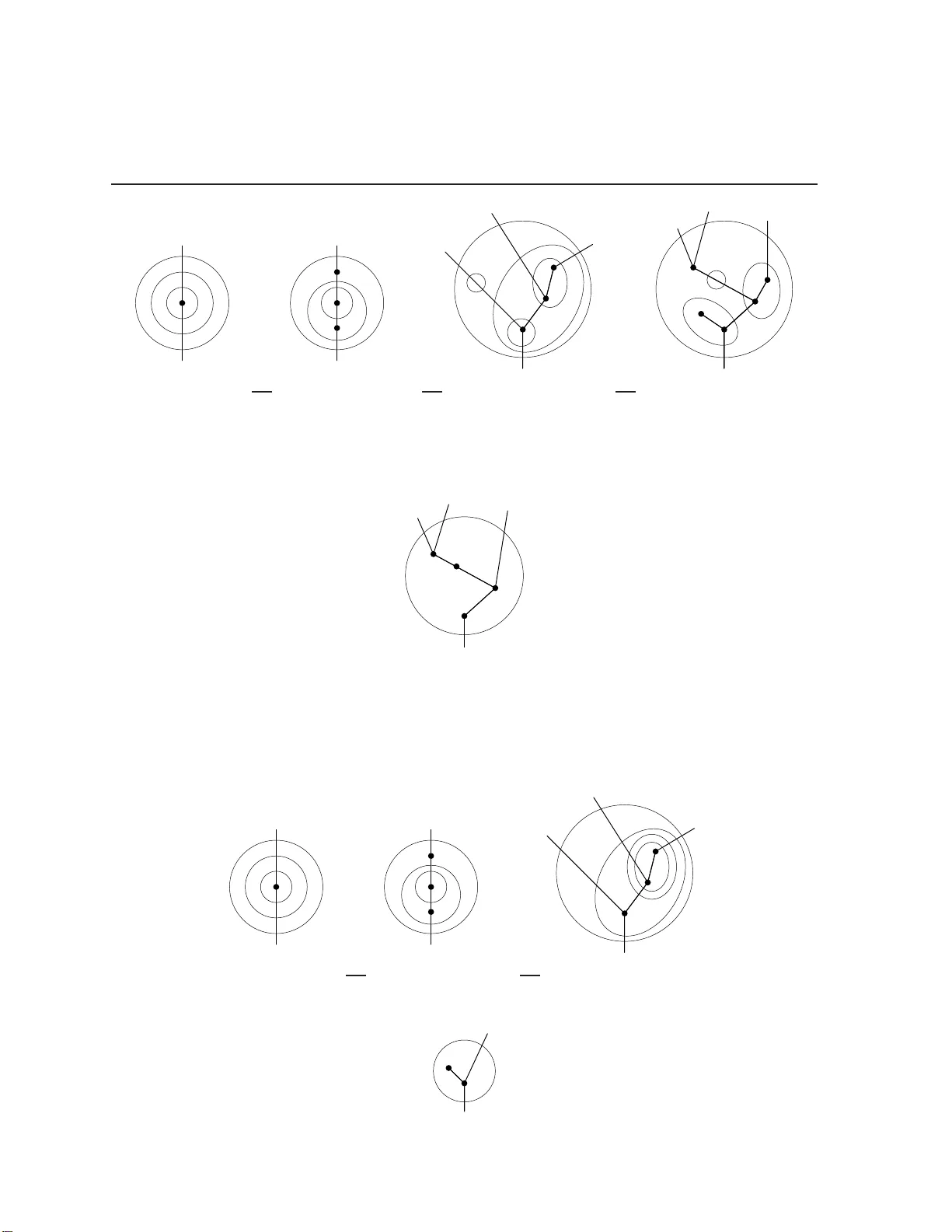
zoom. tex 2010- 02-20 00:59 [1/54] Polynomial functors and op etopes J O A C H I M K O C K , A N D R É J O YA L , M I C H A E L B A TA N I N , and J E A N - F R A N Ç O I S M A S C A R I Abstract W e give an e lementary and direct combinatorial deﬁnition of op etope s in ter ms of trees, well-suited for graphical manipulation and explicit computation. T o rela te our deﬁnition to t he classical d eﬁnition, we recast the Baez-D olan s lice construc- tion for operads in terms of po lynomial monads: our opetopes appear naturally as types for polynomial monads o btained by iterating the Baez- Dolan c onstruction, starting with t h e tr ivial monad. W e show that our notion of o p etope agrees with Leinster ’s. Next we observe a s uspens ion operation for opet opes, and de ﬁne a no - tion of stable o petope s. Stable opetop es form a least ﬁxpoint for the Baez-Dolan construction. A ﬁnal section is devote d t o example computations, and indicates also how the calc ulus of opetop es is well-suited for machine implementation. Introduc t ion Among a dozen or so existing deﬁnitions of weak higher categories, the opetopic ap- pr oach is one of the most intriguing, since it is based on a collection of ‘shapes’ that had not previous ly been studied: the opetopes. Opetopes are combinatorial struct ur es parametrising higher -dimensional many-in/one-out operations, and can be seen as higher -dimensional generalisations of trees. They are important combinatorial struc- tur es on their own, ‘as pervasive in higher -dimensional algebra as simplices ar e in geometry’, according to Leinster [14, p.2 16]. Opetopes and opetopic higher categories wer e introduced by Baez and Dolan in the seminal paper [1], and the theory has been developed further by Hermida-Makkai-Power [9], Leinster [14], Cheng [2], [3], [4], [5], and others. It is in a sense a theory fr om scratch, compared to several other theories of higher categories which build on large bodies of preexisting machinery and experi- ence, e.g. simplicial methods. The full potential of the opetopic approach may depend on a deepe r understanding of the combinatorics of opetopes. At the confer ence on n-categories: Founda tions and applications at the IMA in Min- neapolis, June 2004, much time was de dicated to opetopes, but it be came clear that a concise and direct deﬁnition of opetopes was lacking, and that ther e was no practical way to repr esent higher-dimensional opetopes on the blackboar d. In fact, ther e did not seem to exist a general m e thod to repr esent concr ete opetopes in any way , algebraic, zoom. tex 2010- 02-20 00:59 [2/54] graphical, or by machine. 1 The best deﬁnitions are very abstract and not very hands- on: e.g. Leinster ’s deﬁnition in terms of iterated fr ee cartesian monads [14], or the Hermida-Makkai-Power [9] deﬁnition of opetopic sets (there called multitopic sets), followed by a theor em that this category is a presheaf category , hence characterising a category of opetopes (there called multitopes). As to graphical r epresent ations of opetopes in low dimensions, the current method is based on a polytope interpretation of opetopes (which is at the origin of the ter- minology: the wor d ‘opetope’ comes fro m ‘operation’ and ‘polytope’). Leinster [14, § 7.4] has constructed a geometric realisation functor which pro vides support for this interpr etation, although the p olytopes in general cannot be piece-wise linear objects in Euclidean space. Mor eover , geometrical objects in dime nsion higher than 3 are inher- ently difﬁc ult to repr esent graphically , and curr ently one reso rts to Lego-like drawings in which the individual faces of the polytopes are drawn separately , with small arrows as a recipe to indicate how they are supposed to ﬁt together . The goal of this pape r is to come closer to the combinatorics. Our initial idea was to r epr esent an opetope as a tr ee with some circles, which we now call constell ations . This works in dimension 4 (cf. 1.11 below), but it does not seem to be suf ﬁcient to captur e the possible opetopes in dimension 5 and higher . Pursuing the idea, what we eventually found was a r epresent ation in terms of a seq ue nce of trees with cir cles, and in fact it is basically the notion of metatree originally proposed by Baez and Dolan. That notion was never really developed, though: in the original p a per [1] the claim that metatrees could express opetopes was not really substantiated, a nd in the subsequent literatur e ther e seems to be no mention of the metatr ee notion. The presence of cir cles makes a conceptual differ ence, and it also reveals a certain shortcoming in the original notion of metatree, r elated to units (cf. 1.21). W e hasten to point out that our notion of opetope coincides with the notion due to Leinster [14] (cf. the e xplicit comparison culminating in Theorem 3.1 6 ), not with the original Bae z-Dolan deﬁnition: we work consistently with non-planar trees, which means our opetopes are ‘un-order ed’ like a bstract geometric objects, whereas the orig- inal Baez -Dolan opetopes come equipped with an ordering of their faces. In our ver- sion, the plana r aspect is only a particular featur e of low dimensional opetopes. While our opeto pes agr ee with Leinster ’s, the description we provide is completely elementary and does not even make refer ence to category theory . W e think that our 1 In f act a method d oes e xist for algebraic/mechanical representation: Hermida-M akkai-Power [9, ﬁnal section] explain how any opetope (there called multitope) in arbitrary dimension can be serialised into a string of hash signs a nd stars, with two sorts of brackets. W e shall not go any further into that notation, but jus t to illustrate its ﬂavour , here is the representation of the 3- opetope in 1.9: pp # qp # qp # q [ ⋆ ] qpp # qp # q [ ⋆ ] qpp # q [ ⋆ ] q [ # ] [ # ] p [ ⋆ ] qpp # q [ ⋆ ] q [ # ] W e refer to [9] for instructions on how to parse this. zoom. tex 2010- 02-20 00:59 [3/54] description can serve as the famous ‘5-minute de ﬁnition’ that was previo usly missing, and that it can provide a convenient tool for communicating opetopical ideas. W e also indicate how our approach is well-suited for machine manipulation. Opetopes were intro duced to parametrise higher-dimensional substitutio n oper- ations. Surprisingly , opetopes arise also in another way , name ly from computads and higher-dimensional pasting theory , and we wish to mention that a very differ - ent combinatorial approach ha s been developed in this setting by Palm [15]. A com- putad is a strict ω -category which is dimension-wise free. This notion was devised by Str eet [18] as a tool for describing higher -dimensional compositions in strict n - categories. In the works of Johnson [10] a nd Power [16], [17], differ ent combinatorial and topological repr esentat ions of computads (called pasting schemes) were given, starting fro m Bénabou’s p a sting diagrams for 2-categories a n d the dual graphical lan- guage of string diagrams. The subtleties encounter ed are related with the fact that the category of computads is not a presheaf category . A computad is called many-to-one if the codomain of every indeterminate in dimension k + 1 is itself an indeterminate (in d im e nsion k ). Harnik, Makkai and Zawadowski [8] e stablished an equivalence of categories between many-to-one computads and multitopic sets. In particular , the cat- egory of many-to-one computads is a presheaf category . Palm [15 ] ha s given a purely combinatorial de scription of this presheaf category . He introduces a notion of den- droto pes , certain decorated Ha sse diagrams, and shows that dendroto pic sets (their pr esheaves) are equivalent to many-to-one computads. Hence, by the theorems of Harnik-Makkai-Zawadows ki and Hermida-Makkai-Power , dendrot opes should cor - r espond to opetopes. However , a direct combinatorial comparison has not been given at this time. Let us brieﬂy outline the or ganisation of the exposition. In the ﬁrst section we give the deﬁnition of opetopes in a direct combinatorial way , without refer ence to cate- gory theory . The crucial ingr edient is the corr espondence between non-planar tr ees and nestings of circles: an opetope is merely a sequence of such corr espondences, with an initial condition. W e give the deﬁnition in two steps: ﬁrst the elementary ‘5 -minute deﬁnition’ with example s, then we develop the involved notions of trees a nd constel- lations mor e formally and compare with Baez -Dolan metatr ees. It is possible to jump dir ectly fro m the ‘5-minute deﬁnition’ to Section 5, wher e the same elementary and hands-on approach is pursued to describe in detail how to compute sources and tar- gets of opetopes, and how to compose them. However , such a reading would ignore the theoretical justiﬁcation for the de ﬁnitions and constructio ns. In Section 2 we review some basic facts about polynomial functors, notably their graphical interpretation which is the key point to relate the formal constructio ns with explicit combinatoric s. Section 3 forms the theoretical he a rt of this work: we give an easy account of the Baez-Dolan slice constr uction in the sett ing of polynomial monads. From the graphical zoom. tex 2010- 02-20 00:59 [4/54] description of polynomial functors we see that the Baez-Dolan constructio n is about certain decorated tr ees. The double Baez-Dolan constructio n gives trees decorated with trees, subject to complicated compatibility conditions. W e show that these com- patibility conditions are completely encoded by drawing circles in trees. Iterating the Baez-Dolan constr uction involves the corr espondence between trees and nestings, and it readily follows (Theorem 3.13) that the opetopes de ﬁned in Section 1 arise precisely as types for the polynomial monads produced by iterating the Baez-Dolan construc - tion, starting from the trivial monad. W e compar e the polynomial B a ez-Dolan con- stru ction with Leinster ’s version of the Bae z-Dolan constructio n, and conclude (Theo- r em 3 .16) that our notion of opetope agrees with Leinster ’s [14]. In the short Section 4, we observe a suspension operat ion for opetopes, and deﬁne a notion of stable opetopes. The stable opetopes also form a polynomial monad, and we show this is the le ast ﬁxpoint for the Baez-Dolan constructio n (for pointed monads). In Section 5, we show by way of examples how the calculus of opetopes works in practice: we are concerned with computing sources and targ et of opetopes, and with composing them. In the Appendix we brieﬂy describe a machine implementation of the ‘calculus of opetopes’ based on XML, including a mechanism for automated graphical output. Acknowledgements. W e are grateful to John Baez and Peter May for organising the very inspiring workshop in Minneapolis, and to Eugenia Che ng and Michael Makkai for patiently telling us about opetopes at that occasion. W e are grateful to editors and r efer ees for their attentiveness. W e thank our respective ﬁnancing institutions: the r esearc h of A . J. was supported by the NSERC ; M. B. was supported by the Australian Research Council; J.-F . M. was supported by a grant fr om the CNR in the framewor k of an IMA-CNR collaboration; J. K., curr ently supported by grants MTM2006-11391 and MTM2007-63277 of the Spanish Ministry of Ed ucation and Science, was previous ly supported by a grant fro m the C I RGET at the U QAM a nd insisted on including this opetope drawing, as expression of his gratitude and admiration: zoom. tex 2010- 02-20 00:59 [5/54] 1 Opetope s W e ﬁrst give the quick deﬁnition of opetope, thro ugh the notions of tree, constellation, and zoom. Afterwar ds we develop these notions mor e carefully . The ‘5-minute deﬁnition’ of opetope 1.1 T rees. The fundamental concept is that of a tree. Our tr ees are non-planar ﬁnite r ooted tr ees with boundary: they have any number of input edges (called leaves), and have precisely one output edge (called the r oot edge) always drawn at the bottom. Ther e is a partial or der in which the root is the maximal element and the leaves a re minimal elements. The following d rawings should sufﬁce to exemplify tr ees, but be- war e that the planar aspect inher ent in a drawing should be disregar ded: A formal deﬁnition of tree is given in 1.14. An alternative formalism is developed in [12]. 1.2 Nestings. A nother graphical repr esentat ion of the same structur e is given in terms of nested cir cles in the plane. W e prefer to talk about nested sphe res in space to avoid any idea of planarity when in a moment we combine the notion with tr ees. A nesting is a ﬁnite collection of non-inters ecting spher es and dots, which either consists of a single dot (and no spher es) or has one out er spher e, cont aining all the other spheres and dots. The dots of a nesting correspond to the leaves of the tr ee. The outer sphere cor - r esponds to the root edge of the tr ee, and the special case of a nesting which consists solely of one dot corr esponds to the dotless tr ee. The partial or der is simply inclusion. The following d rawings of nestings corr espond exactly to the ﬁve tr ees drawn above. 1.3 Correspondences. A correspondence between a nesting S and a tr ee T consists of speciﬁed bijections dots ( S ) ↔ leaves ( T ) spher es ( S ) ↔ dots ( T ) zoom. tex 2010- 02-20 00:59 [6/54] r especting the partial or ders. He r e is a typical pictur e: a b c d e f g a e b f c d g The bijections are indicated by the labels a , b , c , d , e , f , g . 1.4 Constellations. A constellation is a superposition of a tr ee with a nesting with com- mon set of dots, and such that each sphe r e cuts a subtr ee. Here is an example: Mor e pr ecisely , it is a conﬁgurat ion C of edges, dots, and spheres, such that (i) edges and dots form a tr ee (called the underlying tree of C ), (ii) dots and spheres form a nesting (the underly ing nes ti ng of C ), (iii) for each sphere, the e dges and dots contained in it form a tree again. A pur ely combinatorial deﬁnition of constellation is given in 1.18. Let us brieﬂy take a look at some de generate examples. In a constellation without a sphere, the underlying nesting is necessarily a single dot. Hence the possibilities in this case are exhausted by the set of tr ees with only one dot: etc. In a constellation without dots, the underlying tr ee must be a single e dge. There must be an outer spher e, so such constellations may look like these examples: zoom. tex 2010- 02-20 00:59 [7/54] Note that every sphere must contain a segment of a line, since there is no such thing as the emp ty tr ee. Finally , we draw a few examples of constellations without leaves: In 3.6 it is shown that constellations repr esent, in a precise sense, trees of tr ees, which is the reason for their importance. W e want to iterate the idea of tr ees of trees by r epeating the step of drawing spheres. T o do this, we shift the nesting to a tree and iterate. In our terminology , we zoom: 1.5 Zooms. A zoom from constellation A to constellation B , written A ❞ s B , is a corr espondence between the underlying nesting of A and the underlying tree of B . In other words, there are speciﬁed two bijections: dots ( A ) ↔ leaves ( B ) spher es ( A ) ↔ dots ( B ) r especting the partial or ders. Here is a n example: 7 6 5 4 2 1 3 8 11 9 10 12 13 14 A B ❞ s 1 2 3 4 5 7 6 9 8 10 14 11 13 12 The bijections are indicated with numbe rs. W e also wish to exhibit the two most degenerate zooms: zoom. tex 2010- 02-20 00:59 [8/54] x ❞ s x x ❞ s x 1.6 Zoom complexes. A zoom complex of d e gr ee n ≥ 0 is a sequence of zooms X 0 ❞ s X 1 ❞ s X 2 ❞ s X 3 ❞ s . . . ❞ s X n . 1.7 Opetopes. An opetope of dimension n ≥ 0 is deﬁned to be a zoom complex X of degr ee n starting like this: X 0 ❞ s X 1 ❞ s X 2 (1) Here, X 0 and X 1 ar e exactly as drawn, while X 2 is described verbally as having one dot and one leaf (necessary in order to be in zoom relation with X 1 ), and having any ﬁnite number of linearly nested spheres. (W e consider two opetopes the same if they only diff er by the names of the involved eleme n ts.) 1.8 Rem a rk. This de ﬁnition of opetope should be attributed to Baez and Dolan [1] who intr oduced the n otion of opetope in terms of a slice constructio n for symmetric operads (a polynomial analogue of which we shall call the Baez-Dolan construction (Section 3)), and off er ed an al ternative description in terms of sequences of trees called metatrees. Deﬁnition 1.7 featur es important adjustments to the Baez-Dolan notion of me tatr ee, as we shall explain in 1.21 1.9 Exam ples. A 0-opetope is the zoom complex (ther e is only one such), and a 1- opetope is the zoom complex ❝ r (again ther e is only one such). The 2-opetopes ar e in bijection with the natural numbers, counting the linearly nested spheres in X 2 . For n ≥ 3, there are no restrictio ns on the constellations X n , except to be in zoom r elation with X n − 1 . For example, if ther e are n spheres in X 2 , then the zoom condition for ces X 3 to be a straight line with n dots on (and the bijection be tween sphe r es and dots is uniq ue ly determined since the line a r nesting of the spheres in X 2 must corre- spond to the line ar arrangement of the dots in X 3 ), and any nesting can be drawn on top of that. Here is an example: zoom. tex 2010- 02-20 00:59 [9/54] X 0 ❞ s X 1 ❞ s X 2 ❞ s X 3 Clearly the information encoded in X 0 , X 1 and X 2 is redundant, and a 3-opetope is completely speciﬁed by a X 3 of this form: a line with dots and ‘ sphe res’. This is equivalent to specifying a planar tr ee. The planarity comes about be cause ther e is a line or ganising the dots in X 3 , which in turn is a consequence of the linear nesting of the spher es in X 2 . Here is the planar tree corr esponding to the 3-opetope above: and her e is how this 3-opetope would be repr esented in the p olytope style, as in Lein- ster ’s book [14] a nd in the work of Cheng: 1.10 Rem ark. The two-step initial condition in the deﬁnition of opetope may look strange, and in any case the ﬁrst two constellations are r edundant in terms of informa- tion. (As we just saw , for n ≥ 3 also X 2 is redundant, since the conﬁguratio n of dots in X 3 completely determines X 2 .) The justiﬁcatio ns for including X 0 and X 1 ar e ﬁrst of all to cover also dimension 0 and 1 in an uniform way , and make the opetope dimension match the degree of the complex. Second, those leading will play a key role in the notion of stable opetopes in 4.1. From the theor etical viewpoint, which we take up in the next section, the point is that X 0 and X 1 r epr esent the trivial polynomial functor (the identity functor on Set ), from which iterated application of the Bae z -Dolan con- stru ction (3.1) will generate all the opetopes in higher dimension, cf. Theorem 3.13. The extra condition imposed on X 2 (the linear nesting of the spheres) is also explained by that construc tion. The fact that ther e a re no extra conditions on X n for n ≥ 3 ex- pr esses a remarkable feature of the double Baez -Dolan construction, at the heart of this paper , namely that the double Baez-Dolan construct ion generates constellations, cf. Theorem 3.6. zoom. tex 2010- 02-20 00:59 [10/5 4 ] 1.11 Exam ple. A 4-opetope is a zoom complex of d e gr ee 4 like this example: Y 0 ❞ s Y 1 ❞ s b a Y 2 ❞ s a r q b s p Y 3 ❞ s s b q r p a Y 4 As discussed, it would be enough to ind icate Y 3 ❞ s Y 4 , a nd if we furthermor e take advantage of the linear order in Y 3 and make the convention that Y 4 should be a planar tr ee, whe r e the clockwise planar order expresses the (downwards) linear or der in Y 3 , then also Y 3 is redundant, and we can repr esent the 4-opetope by the single constella- tion: s p b a q r Y 4 (While such economy can sometimes be practical, conceptually it is rather a n obfusca- tion.) 1.12 Exam ple. W e ﬁnish with an example of a 5-opetope, just to point out that ther e is no longer any na tural planar structur e on the underlying trees in d e gr ee d ≥ 5. Arg u- ing as above, to specify a 5-opetope it is enough to specify a single zoom Z 4 ❞ s Z 5 , pr ovided we unde rstand that the tr ee in Z 4 is planar (and he nce allows us to recon- stru ct the pr evious constellation). Here is an e xample of a 5-opetope r epresent ed in this economical manner: p x y b c a Z 4 ❞ s a b c p y x Z 5 zoom. tex 2010- 02-20 00:59 [11/5 4 ] Formal deﬁni t ions: trees and constellations While the p resented deﬁnition of opetopes is appealing in its simplicity , scrutiny of the deﬁnition raises some questions: what exactly is meant by tr ee? Is it a combinatorial notion? In that case, what does it mea n to draw circles on a tree? And when we say ‘tr ee’, ‘const ellation’, or ‘opetope’, do we r efer to concrete speciﬁc sets with str uctur e or do we refer to isomorphism classes of such? In this subsection we give the deﬁnitions a mor e formal treatment. W e show in particular that the notion of constellation is pur e ly combinatorial and does not depend on geometric r e a lisation. Secondly , the analysis will clarify the r elation to Baez-Dolan metatr ees (and uncover the shortcoming with these). Thir dly , the insight provided by the formal viewpoint will be helpful for understanding the constructio ns in Section 3 and the calculations in Section 5. The question of explicit-sets-with-st ructur e versus their isomorphism classes de- serves a remark before the deﬁnitions. W e want to deﬁne the various notions (trees, constellations, zoom complexes, opetopes) in terms of ﬁnite sets with some structur e, in or der to classify as combinatorial n otions. As such these objects form a pr oper class. On the other ha n d , na turally we ar e mostly interest e d in these struct ur e s up to isomor - phism. Our choice will be to stick with the e xplicit ﬁnite-sets-with-str ucture as long as the objects ma y possess non-trivial automorphisms (which is the case for tr e e s, con- stellations, and z oom complexes), but consider isomorphism classes for rigid objects like P -tr ees (trees decorated by a polynomial endofunctor P , as intr oduced in 2.8) and opetopes. Hence an opetope will be de ﬁned as a set of isomorphism classes of certain (rigid) object s (this was implicit in 1.7, and in particular there will be only a small set of them. This is in accor dance with pr evious deﬁnitions of opetopes in the literatur e — in fact this issue had not previously come up since ther e was no combinator ia l description available. 1.13 Grap hs. By a graph we understand a pair ( T 0 , T 1 ) , where T 0 is a set, and T 1 is a set of subsets of T 0 of car dinality 2. The e lements in T 0 ar e called vertices , and the elements in T 1 edges . An edge { x , y } is said to be incident to a vertex v if v ∈ { x , y } . W e say a vertex is of valence n if the set of incident edges is of cardinality n . The geometric realisation of a graph is the CW -complex with a 0-cell for each vertex, and for each edge a 1-cell attached at the points correspo nding to its two incide nt vertices. 1.14 T rees. By a ﬁ nite rooted tree with boundary we mean a ﬁnite graph T = ( T 0 , T 1 ) , connected and simply connected, equippe d with a pointed subset T . of vertices of va- lence 1, called the boundary . W e will not need other kinds of tr ees than ﬁnite r ooted tr ees with boundary , and we will simply call them trees . (An alternative tree for ma lism is de veloped in [12].) The basepoint t 0 ∈ T . is called the output verte x , and the remaining vertices in T . ar e zoom. tex 2010- 02-20 00:59 [12/5 4 ] called input vertices . Most of the time we shall not refer to the boundary vertices at all, and graphically a boundary vertex is just repr esented as a loose end of the incident edge. Edges incident to input vertices ar e called leaves or input edges of the tree, while the uniq ue edge incident to the output vertex is called the root ed g e or the output ed g e of the tr e e. The vertices in T 0 r T . ar e called nodes or dots ; we draw them as dots. A tr ee may have zero dots, in which case it is just a single edge (together with two boundary vertices, which we suppr ess); we call such a tr ee a unit tree . Not every vertex of valence 1 needs to be a boundary vertex: those which are not are called null-dots . unit tree null-dot → ← leaf root edge → The standard graphical repr esentation of tr e e s is justiﬁed by geometric realisation. Note that leaves and root ar e realised by half-open intervals, and we keep track of which are which by always drawing the ro ot at the bottom. An isom orphism of trees is an isomorphism of the underlying graphs pr e serving ro ot and leaves. A tr ee can be recov e r e d up to isomorphism by its geometric realisation. W e shall fr e quently be interested only in the isomorphism classes. This was implicit in the ‘5 -minute’ de ﬁnition. If T = ( T 0 , T 1 , T . , t 0 ) is a tr e e, the set T 0 has a natural poset struc ture a ≤ b , in which the input vertices and null-dots are minimal elements and the output vertex is the maximal eleme nt. W e say a is a child of b if a ≤ b and { a , b } is an edge. Ea ch dot has one output edge, and the remaining incide nt edges are called input edges of the dot. 1.15 Nestings and correspondences. Nestings (as in 1.2) a re just another graphical r ep- r e se ntation of an abstract tr ee ( T 0 , T 1 , T . , t 0 ) . Graphically , a nesting is a collection of non- intersecting spher e s and dots, which either consists of a single dot (and no spheres) or has one outer sphere, containing all the other spheres and dots. W e identify two nest- ings if ther e is a n isotopy between them. W e shall need some more terminology about nestings, expanding the dictionary between trees and ne stings. A sphere that does not contain any other spher es or dots is called a null-sphe re . These corr e spond exactly to the null-dots of a tree. The region bounded on the outside by a sphere S and on the inside by the dots and spheres contained in S is called a layer . The layers of a nesting corr espond to the nodes of the tree. An inner sphe re me d iates between two layers just like an inner edge in a tr ee sits between two nodes. W e will often confuse a la yer with its outside bounding sphere. 1.16 T owards a combinatorial deﬁnition of constellations. In 1.4 we d e ﬁned a con- stellation as a tree with a sphere nesting on top, more precis e ly as a conﬁguration C of edges, dots, and spheres (in 3-space), such that: (i) edges and dots form a tree, (ii) zoom. tex 2010- 02-20 00:59 [13/5 4 ] dots and spher e s form a nesting, and (iii) for ea ch sphere, the edges and dots co ntained in it form a tr ee again. This deﬁnition has a clear intuitive content, and pla ys an im- portant role as convenient tool for manipulating constellations and opetopes, just like we usually manipulate trees in terms of their geometrical aspect, not in terms of ab- stract graphs. However , the deﬁnition depends on geometric realisatio n, and it is not clear at this point of our exposition that it is a rigor ous notion at all. It is likely that the de ﬁnition can be formalised geometrically by talking about isotopy classes of such conﬁguratio ns of (progr essive) line segments, dots, and spheres in Euclidean space. W e shall not go further into this. W e wish instead to str ess that the notion can be given in purely combinatorial terms. The ide a is to captur e the struct ure by specifying some bijections between the underlying tr ee and the tree corr esponding to the nesting. For this to work it is necessary to mark the position of the null-spheres by temporarily turning them into dots. This is formalised throug h the notion of subdivision of tr e es: 1.17 Subd ivision and ke rnels. A li near tree is a tree in which every dot has exactly one input edge. The unit tree is an example of a linear tree. (Up to isomorphism) there is one linear tree for each natural number . A subdivis ion of a tree T is a tree T ′ obtained by replacing e ach e d ge by a linear tree. W e draw the new dots as white dots. Here is a pictur e of a tr e e and a subdivision: T T ′ (2) When we speak about dots of a subdivided tree we mean the union of old and new dots: dots ( T ′ ) = blackdots ( T ′ ) + whitedots ( T ′ ) (note that blackdots ( T ′ ) = dots ( T ) ). If T is a tr ee , every subset K ⊂ dots ( T ) spans a full subgraph K † , whe r e an edge of K † is a n edge of T connecting two nodes of K . W e call K a kernel if the graph K † is non-empty and connected. A kernel K spans a tree with boundary K ‡ , whose edges ar e those of T adjacent to a n element of K ; the dots of K ‡ ar e the elements of K and the boundary vertices of K ‡ ar e those vertices of K † not in K . In other wor d s, a sphere containing exactly the dots of a kernel cuts a tr ee, as in condition (iii) of 1.4. I n the following picture, K = { r , u , v } is an example of a kernel, K † is indicated with fat edges, a nd the tr ee K ‡ is what’s inside the spher e : zoom. tex 2010- 02-20 00:59 [14/5 4 ] r u v (When we speak of kernels of a subdivided tr ee we refer to all dots, black and white.) 1.18 Combinatorial deﬁnition of constellation. A constellation C : T → N between two tr ee s T a nd N is a triple ( T ′ , σ • , σ ◦ ) , whe r e T ′ is a subdivision of T , a nd σ • and σ ◦ ar e bijections σ • : blackdots ( T ′ ) ∼ → leaves ( N ) σ ◦ : whitedots ( T ′ ) ∼ → nulldots ( N ) such that the sum ma p σ : = σ • + σ ◦ satisﬁes the kernel rule : for e ach x ∈ dots ( N ) , the set { t ∈ dots ( T ′ ) | σ ( t ) ≤ x } is a kernel in T ′ . (3) An isomorphism of constellations consists of isomorphisms of the unde rlying (subdi- vided) trees compatible with the structural bijections. Here is a picture of a constellation in this sense: a b x y z T C − → p q a b x y z N (4) (The white dots are not a part of T ; they r e pr e sent the subdivision of T which is a part of the data constitut ing C .) Let us compare the deﬁnition of constellation given in 1.18 with the drawings of 1.4, justify ing that the latter constitute a faithful graphical r epresentation of the former . Given a constellation accor ding to de ﬁnition 1.18, as in Figur e (4), for each dot x in N that is not a null-dot, draw a sphe r e in T ′ ar ound those dots in T ′ corr esponding to the descendant le aves and null-dots of x in N , as in the kernel rule (3). The kernel rule tells us that this sphere cuts a tree (as in 1.4). The spher e must be drawn inside the spher e corresponding to the parent node of x (if any); this ensures that the spheres are non-intersecting and that the result ing nesting corresponds to the tr ee N . (Name the zoom. tex 2010- 02-20 00:59 [15/5 4 ] spher e s and white dots in T ′ by the corresponding dots in N .) T o ﬁnish the construc - tion, r epla ce the white dots in T ′ by null-spheres. a b x y z C T p q a b N x y z (5) It is now clear that the left-hand side of the pictur e is a constellation in the sense of 1.4. (Note that if N ha s no dots, then in particular it has no null-dots, so T = T ′ . Furthermor e in this case N must have p recisely one leaf, so T has just one dot and is ther efore a constellation even without any spher es drawn.) Conversely , given an constellation C in the sense of 1 .4, with underlying tree T , C T the pr e ceding ar guments can be r eversed to constr uct a constellation a ccording to the combinatorial deﬁnition 1.18: ﬁrst draw the tr ee N corr esponding to the unde rlying nesting of C (using the spheres as names for the dots in N ) (this gives Figure (5)), then erase all the spheres in C except the null-spheres, and draw the null-spheres so small that they look like (white) dots — they constitute now a subdivision of T . At this point we have a constellation in the sense of 1.18: the bijections σ • and σ ◦ ar e already part of the corr espondence between the underlying nesting of C and the tr ee N , and each dot x ∈ dots ( N ) corr esponds to a sphere in C , so the kernel rule (3) is just a reformulatio n of the condition that e ach sphere cuts a tree. It is clear that a constellation in the sense of 1.18 can be recover ed uniquely fr om its 1.4-interpr etation. 1.19 Zooms a nd zoom complexes, revisited. Now that the notion of constellation has been formalised, the deﬁnitions of zoom (1.5) and zoom complex (1.6) are already for - mal. L et us unravel these notions by p lugging in the combinatorial deﬁnition of con- stellation (1.1 8 ). Given a zoom zoom. tex 2010- 02-20 00:59 [16/5 4 ] a b x y z C 1 ❞ s a b x y z C 2 the formal deﬁnition of constellation (1.18) leads to this drawing: a b x y z C 1 − → a b x y z ❞ s a w v u b x y z p q C 2 − → p q x y v u w z The deﬁning pro p e rty of zoom means the two tr ees in the middle coincide (modulo the subdivision, which is rather a part of the str uctur e of C 2 ), so we can overlay the two constellations: a b x y z a w v u b x y z p q p q x y v u w z In conclusion, a zoom is a sequence of thr ee trees connected by constellations: T 0 C 1 − → T 1 C 2 − → T 2 . Similarly , a zoom complex is a sequence of trees a nd constellations T 0 C 1 − → T 1 C 2 − → T 2 · · · T n − 1 C n − → T n . (6) An is om orphism of zoom complex e s is a sequence of isomorphisms of constellations, compatible with the zoom bijections. I n the viewpoint of (6) it is a sequence of isomor- phisms of subdivided trees compatible with the str uctural bijections of 1.18. Note that zoom. tex 2010- 02-20 00:59 [17/5 4 ] a zoom complex of any degree may allow non-trivial automorphisms. For example, the following zoom complex ha s a non-trivial involution: u v ❞ s u v ❞ s u v 1.20 Opetopes, r e visited. W e deﬁned the k -opetopes to be the isomorphism classes of zoom complexes of degree k subject to an initial condition (1.7). Observe that such zoom complexes are rigid objects (i.e. have no non-trivial automorphisms). Indeed, any non-trivial automorphism of a zoom complex C induces a non-trivial automor - phism already on the underlying tree of C 0 because of the structural bijections in the deﬁnition of zoom. C learly the initial condition precludes non-trivial automorphisms in C 0 . W e saw in 1.9 that an opetope of dim e nsion 2 can be r e p resented by a linear tree, and an opetope of d imension 3 by a planar tr ee , which is the same thing as a nesting on a linear tr ee. In other words, an opetope of dimension 3 can be repr esented as a constellation T 2 → T 3 , where T 2 is a linear tree. In general, an opetope of dimension n ≥ 3 can be r e p resented by a sequence of trees and constellations T 2 C 3 − → T 3 C 4 − → · · · C n − → T n , (7) with T 2 a linear tree, or equivalently , as C 3 ❞ s C 4 ❞ s · · · ❞ s C n , (8) wher e C 3 is the constellation associated to a planar tree as in 1 . 9 . The sequence (8) is graphically redundant compared to the seque nce (7), but d rawing the redundant spher e s is very practical as they explicitly witness the validity of the kernel rule (3). 1.21 Relation with Baez-Dolan m etatrees. The viewpoint on zoom complexes given in 1.19 pr ovides an explicit comparison with the notion of metatr ee intr oduced by Bae z and Dolan [1]. There are two important differ ences. A metatree (cf. [1], pp. 176 – 177) is essentially a seque nce of tr ee s T 0 , . . . , T n not al- lowed to have null-dots, with speciﬁed bijections σ • i : dots ( T i − 1 ) ∼ → leaves ( T i ) sat- isfying the kernel rule (3). In other words , it is the special case of a zoom complex wher e the tr ees have no null-dots, and hence there is no subdivision involved in the constellations. Null-dots repr esent nullary operations of the operads or polynomial monads of the Baez-Dolan construct ion 3.1 , and nullary operations do arise. The refor e the Baez-Dolan metatrees seem to be insufﬁcient to reﬂect the Bae z-Dolan construct ion and to describe opetopes. Our zoom complexes may be what Baez and Dolan really envisaged with the notion of metatree. zoom. tex 2010- 02-20 00:59 [18/5 4 ] The second differ ence is of another natur e: Bae z and Dolan worked with planar tr ees, but intr oduced a notion of combed tree , in which the lea ves a re allowed to cr oss each other in any permutation. The trees in B a ez-Dolan metatrees are in fact combed. These artefacts come from working with symmetric operads. The effect on the deﬁ- nition of opetope is that each opetope comes equippe d with an ordering of its faces. W e work instead with non-planar trees and polynomial monads, and the result i ng opetopes (which agree with Leinster ’s, cf. 3.18) are ‘un-or dered’ like abstract geomet- ric objects. Planarity is revealed to be a special feature of dimension 3, cf. 1.9. Let us remark that we think the spheres are an important conceptual device for understanding opetopes in terms of seq ue nces of tr e e s. Baez and Dolan stressed that a key feature of the slice construct ion is that operations are pr omoted to types, and r e d uction laws are promoted to operations. This two-level correspo n d e nce comes to the for e with the notion of zoom: the types are r epresented by the leaves, the operations ar e the dots, and the reduction laws ar e express e d by the sphe res. The zoom relation shifts dots to leaves a n d spheres to dots. 2 Polynom i a l fun c tors and p o lynomial monad s 2.1 Polynomial functors. W e recall some facts about polynomial functors. (Details for the notions needed here can be found in [7]. The manuscript [13] aims at e ventually becoming a more comprehensive refer ence.) A diagram of sets and set maps like this E p ✲ B I s ✛ J t ✲ (9) gives rise to a polynomial functor P : Set / I → Set / J deﬁned by Set / I s ∗ ✲ Set / E p ∗ ✲ Set / B t ! ✲ Set / J . Here lowerstar and lowershriek denote, respectively , the right adjoint and the left ad- joint of the pullback functor upperstar . In explicit terms, the functor is given by Set / I − → Set / J [ f : X → I ] 7 − → ∑ b ∈ B ∏ e ∈ E b X s ( e ) wher e E b : = p − 1 ( b ) and X i : = f − 1 ( i ) , and wher e the last set is considered to be over J via t ! . W e will a lwa ys assume that p : E → B has ﬁnite ﬁbr es. No ﬁniteness conditions ar e imposed on the individual sets I , J , E , B , nor on the ﬁbr es of s and t . zoom. tex 2010- 02-20 00:59 [19/5 4 ] 2.2 Graph ical interpr e tation. The following graphical interpr etation links polynomial functors to the tr ee struc tures of Section 1. (This interpretat ion is not a whim: there is a deeper relationship between polynomial functors and trees, analysed mor e closely in [12].) The important aspects of an element b ∈ B are: the ﬁbre E b = p − 1 ( b ) and the element j : = t ( b ) ∈ J . W e captur e these data by picturing b as a (non-planar) bouquet (also called a cor olla) b j e . . . Hence each leaf is labelle d by an ele me nt e ∈ E b , and each element of E b occurs exactly once. In virtue of the map s : E → I , each leaf e ∈ E b acquir e s furthermor e a n implicit decoration by an element in I , namely s ( e ) . An element in E can be pictured as a bouquet of the same type, but with one of the leaves marked (this m a rk chooses the ele ment e ∈ E b , so this description is merely an expr e ssion of the natural identiﬁcation E = ∐ b ∈ B E b ). Then the map p : E → B consists in forgetting this mark, and s returns the I -decoration of the marked leaf. 2.3 Evaluation of a polynomial functor . Evaluating the polynomial functor P on a n object f : X → I has the following graphical interpretation. The eleme nts of P ( X ) are bouquets as a bove, but where each leaf is furthermor e decorated by e lements in X in a compatible way: b j e · · · x · · · · The compatibility condition for the decorations is that a leaf e ma y have decoration x only if f ( x ) = s ( e ) . The set of such X -decorated bouquets is naturally a set over J via t (return the decoration of the roo t edge). More formally , P ( X ) is the set over B (and hence over J via t ) whose ﬁbre over b ∈ B is the set of commutative triangles X ✛ E b I . s ✛ f ✲ zoom. tex 2010- 02-20 00:59 [20/5 4 ] 2.4 Composition of polynomial functors. The composition of two polynomial func- tors i s again polynomial; this is a consequence of distribut ivity and the Beck-Chevalley conditions [13]. W e are mostly inter ested in the case J = I so that we can compose P with itself. The composite polynomial functor P ◦ P can be described in terms of graft- ing of bouquets: the base set for P ◦ P , formally described as p ∗ ( B × I E ) , is the set of bouquets of bouquets (i.e. two-level trees) b e c . . . The conditions on the individual bouquets are still in for ce: each dot is decorat ed by an element in B , and for a dot with de coration b the set of incoming edges is in speciﬁed bijection with the ﬁbre E b . The compatibility condition for grafting is this: Compatibility Condition : for an edge e coming out of a dot decorated c , we have s ( e ) = t ( c ) . 2.5 Morphisms. A cartesian natural transformation u : P ′ ⇒ P be tween polynomial functors corresponds to a commutative di a gram E ′ p ′ ✲ B ′ I s ′ ✛ J t ′ ✲ E ❄ p ✲ s ✛ B ❄ t ✲ (10) whose middle squa re is cartesian, cf. [13]. In other words, giving u amounts to giving a J -map u : B ′ → B together with a n I -bijection E ′ b ′ ∼ → E u ( b ′ ) for e ach b ′ ∈ B ′ . Let Poly ( I ) denote the category whose objects ar e the polynomial e ndofunctors on Set / I a s in (9) and whose arrows are the cartesian natural transformations as in (10). This is a strict monoidal category under composition, and with the identity functor Id as unit object. Note that a polynomial functor always preserves cartesian squares, and (under the assumption E → B ﬁnite) sequential colimits [13]. 2.6 Polynomial monads. By a polynomial monad we understand a polynomial endo- functor P : Set / I → Set / I with monoid stru ctur e in Poly ( I ) . In other wor ds, there is speciﬁed a composition law µ : P ◦ P → P with unit η : Id → P , satisfying the usual zoom. tex 2010- 02-20 00:59 [21/5 4 ] associativity and unit conditions, and µ a nd η are cartesian natural transfor m a tions. Thr oughout we indicate monads by their functor part, conﬁdent that in each case it is clear what the natural-transfor ma tion part is, or e xplicitating it otherwise. The composition law is described graphically as an operation of contracting two- level tr ees (formal compositions of bouquets) to bouquets. W e shall refer to I as the set of types of P , denoted typ ( P ) , and B as the set of operations , denoted op ( P ) . Since we have a unit, we can furthermor e think of E as the set of parti al operations , i.e . operations all of whose in p uts except one are fed with a unit. The composition law can be described in terms of partial operations as a map B × I E → B , consisting in substituting one operation into one input of another operation, provided the types match: t ( b ) = s ( e ) . 2.7 The free monad on a polynomial endofunctor . (See also Gambino-Hyland [6].) Given a polynomial end ofunctor P : Set / I → Set / I , a P -set is a pair ( X , a ) whe re X is an object of Set / I a n d a : P ( X ) → X is an arro w in Set / I (not subject to any further conditions). A P -map fr om ( X , a ) to ( Y , b ) is an arr ow f : X → Y giving a commutative diagram P ( X ) P ( f ) ✲ P ( Y ) X a ❄ f ✲ Y . b ❄ Let P -Set / I de note the category of P -sets and P -maps. The forgetf ul functor U : P -Set / I → Set / I ha s a left adjoint F , the free P-se t functor . The monad P ∗ : = U ◦ F : Set / I → Set / I is the free m onad on P . This is a polynomial monad, and its set of operations is the set of P -trees, as we now explain. 2.8 P -trees. Le t P d enote a polynomial e ndofunctor given by I ← E → B → I . W e deﬁne a P -tree to be a tr ee whose edges are decorated in I , whose nodes are d ecorated in B , and with the additional struct ure of a bijection for e a ch node n (with decoration b ) between the set of input edges of n and the ﬁbre E b , subject to the compatibility condition that such an edge e ∈ E b has decoration s ( e ) , and the output edge of n has decoration t ( b ) . Note that the I -de coration of the e dges is completely d etermined by the node decorat ion together with the compatibilit y r e quir e ment, except for the case of a unit tree. zoom. tex 2010- 02-20 00:59 [22/5 4 ] Another description is useful: a P -tree is a tr ee with ed ge set A , node set N , and node-with-marked-input-edge set N ′ , together with a d ia gram A ✛ N ′ ✲ N ✲ A I α ❄ ✛ E ❄ ✲ B β ❄ ✲ I . α ❄ Then the vertical maps α and β expr ess the de corations, and the commutativity and the cartesian condition on the middle square express the bijections an d the compatibility condition. The top ro w is a polynomial functor associated to a tree, and in short, a P -tree can be seen as a cartesian morphism fr om a tr ee to P in a certain category of polynomial endofunctors [12]. An isomorphism of P -trees is an isomorphism of tr ees co mpatible with the P -decorations. It is clear that P -trees are rigid Denote by tr ( P ) the set of isomorphism classes of P - tr ees. This is the set of formal combinations of the operations of P , i.e . obtained by fr ee ly gr a fting elements of B onto the leaves of elements of B , provided the decorations match (and formally adding a unit tree for each i ∈ I ). The set tr ( P ) has a natural map to I by r e turning the root , and it can be described as a least ﬁxpoint for the polynomial endofunctor Set / I − → Set / I X 7− → I + P ( X ) ; as such it is given explicitly as the colimit tr ( P ) = [ n ∈ N ( I + P ) n ( ∅ ) . 2.9 Explicit de scription of the free monad on P . A slightly more general ﬁxpoint constr uction characterises the free P -set monad P ∗ : if A is an object of Set / I , then P ∗ ( A ) is a le a st ﬁxpoint for the endofunctor X 7 → A + P ( X ) . In e xplicit terms, P ∗ ( A ) = [ n ∈ N ( A + P ) n ( ∅ ) . It is the set of (isomorphism classes of) P -tr ees with leaves de corated in A . But this is exactly the characterisation of e valua tion of a polynomial functor (2.3) with operation set tr ( P ) : let tr ′ ( P ) denote the se t of (isomorphism classes of) P -trees with a marked leaf, then P ∗ : Set / I → Set / I is the polynomial functor given by tr ′ ( P ) ✲ tr ( P ) I ✛ I . ✲ zoom. tex 2010- 02-20 00:59 [23/5 4 ] The maps are the obv ious ones: return the ma rked leaf, for get the mark, and r eturn the r oot edge, respectively . The monad struct ure of P ∗ is d e scribed explicitly in terms of grafting of trees. I n a partial-composition description, the composition law is tr ( P ) × I tr ′ ( P ) → tr ( P ) consisting in grafting a tree onto the speciﬁed input leaf of another tree. The unit is given by I → tr ( P ) associating to i ∈ I the unit tree with ed ge de corated by i . (One can r e a dily check that this monad is cartesian.) 3 The Bae z -Dolan constru ction for polyn o mial monads Thr oughout this section, we ﬁx a polynomial monad P : Set / I → Set / I , repr esented by E ✲ B I ✛ I . ✲ W e shall associate to the p olynomial monad P : Set / I → Set / I another p olyno- mial monad P + : Set / B → Set / B . The idea of this construct ion is due to Baez and Dolan [1], who r e a lised it in the settings of symmetric operads. W e ﬁrst give a very explicit version for polynomial monads, and show how to produce the opetopes from it by iteration, recovering the elementary deﬁnition of opetopes given in 1 .7. I t is the graphical interpretation of polynomial functors that allows us to extract the combina- torics. Afterwar ds we compare with L e inster ’s deﬁnition of opetopes [14, §7.1]. This is just a que stion of comparing our version of the Baez-Dolan constru ction with Le in- ster ’s; the iterative constr uction of opetopes is exactly the same . Explicit constructi on 3.1 The Baez-Dolan construction for a polynomial monad. Starting from our poly- nomial monad P , we de scribe explicitly a ne w polynomial monad P + , the Baez-Dolan construction on P . The idea is to substitute into dots of trees instead of grafting at the leaves (so notice that this shift is like in a zoom r e la tion). Speciﬁcally , deﬁne tr • ( P ) to be the set of (isomorphism classes of) P -trees with one marked dot. There is now a polynomial functor tr • ( P ) ✲ tr ( P ) B ✛ P + B t ✲ zoom. tex 2010- 02-20 00:59 [24/5 4 ] wher e tr • ( P ) → tr ( P ) is the forgetful map, tr • ( P ) → B retur ns the bouquet around the marked dot, and t : tr ( P ) → B comes fr om the monad structur e on P : it am ounts to contracting all inner edges (or setting a new dot in a unit tr ee). Graphically: *                         P + t (11) (In this diagram as well as in the following diagrams of the same type, a symbol   is meant to designate the set of all bouquets like this (with the ap p ropriate decoration), but at the same time the speciﬁc ﬁgures r epresenting each set are chosen in such a way that they match under the structur e maps.) Note that since the for getful m a p for gets a marked d ot, the nullary operations in P + ar e precisely the unit trees , one for each i ∈ I . 3.2 Monad structure on P + . W e ﬁrst compute the value of P + on an object C → B of Set / B . Using the explicit graphical description of evaluation of a polynomial functor 2.3, we see that the result is the set of P -tr ee s with each node d ecorated by an eleme nt of C , compatibly with the arity map C → B (being a P -tree means in particular that each node already has a B -decoration; these decorations must match). W e can now compute P + ◦ P + : its set of operations is P + evaluated at t : tr ( P ) → B : that’s the set of (isomorphism classes of) P -trees with nodes decorated by P -tr e e s in such a way that the total bouquet of the decorating tree ma tches the local bouquet of the node it decorates. Similarly , the set of ‘pa rtial operations’ for P + ◦ P + is the set of P -trees-wit h-a-marked-node, the marked node being decorated with a P -tree-with-a- marked-node, and the remaining nodes being decorated by P -tr ees. Now the monad struct ure on P + is easy to de scribe: The composition law P + ◦ P + ⇒ P + consists in substituting e a ch P -tree into the node it decorates. The substitu- tion can be described in terms of a partial composition law tr ( P ) × B tr • ( P ) → tr ( P ) deﬁned by substituting a P -tr e e into the marked dot of a n element in tr • ( P ) , as indi- zoom. tex 2010- 02-20 00:59 [25/5 4 ] cated in this ﬁgur e: F x y z x f y z r e sulting in x y z (12) (The letters in the ﬁgure do not repr e sent the decorations — they are rather uniq ue labels to express the involved bijections, a nd to facilitate comparison with Figur e (13) below .) Of course the substitution makes sense only if the decorations match. This means that t ( F ) , the ‘total bouquet’ of the tree F , is the same a s the local bouquet of the node f . Formally the substitution can be described as a pushout in a category of P -trees, cf. [12]. The unit for the monad is given by the m a p B → tr ( P ) interpreting a bouquet as a tr ee with a single dot. It is readily checked directly that the monad axioms hold. (Alternatively this will follow from the proo f of Theorem 3.16 wher e P + is shown isomorphic to something which is a monad by construct ion.) 3.3 The BD construction in terms of nestings. W e have described the free-monad constr uction and the Baez -Dolan construct ion in terms of trees, but of course they can equally well be described in terms of nested spheres, a s we shall now explain. The interplay between these two descriptions will lead directly to opetopes as deﬁned in Section 1. Let us str ess again that trees and nestings are just diff e r e n t graphical expres- sions of the same combinatorial structur e. However , some fe a tur es of tr ees can be a little bit subtler to see in terms of ne stings. The basic operations, the eleme nts in B , are conﬁgurations of a spher e with dots inside: j e 1 . . . b W e call such a thing a layer . The set of dots inside the spher e is in bijection with the set E b , and via s : E → I these dots also carry an implicit decoration by elements in I , the input types. The la bel j on the outside of the sphere repr e sents t ( b ) , the output. W e put the label b on the inside of the sphere it decorates, since it mediates be tween the zoom. tex 2010- 02-20 00:59 [26/5 4 ] input devices (the dots ) and the output device (the spher e), just as the dot of a bouquet mediates between the inputs (the leaves) and the output. Next, tr ( P ) is the set of (isomorphism classes of) arbitrary P -nestings, with layers decorated in B and spheres and dots decorated in I (subject to compatibility condi- tions), and tr ′ ( P ) is the set of (isomorphism classes of) arbit rary P -ne stings (compatibly decorated) with a m a rked dot. The substitution law for the free monad on P is now described by substituting one P -nesting into a dot of another , pro vided the decorations match. (This corr esponds to grafting of tr ees.) For the Baez-Dolan construct ion (wher e we now suppose P is a monad), tr • ( P ) is the set of (isomorphism classes of) P -nestings with a marked sphere, so here is the nesting version of Figur e (11): *                                     ( ) ( ) P + s t Note that the map t consists in erasing all inner spheres, which is just the ne sting equivalent of the tr ee operation of contracting all inner edges — this is always possible for undecorated ne stings, but for this to make sense in the P -decorated case we ne ed the monad structur e on P . The ma p s consists in r e turning the layer determined by the marked spher e: this means the region delimited on the outside by the marked spher e itself and on the inside by its childr e n, so the operation can also be described as taking the ma rked sphere and contracting each sphere inside it to a dot. (This is the ne sting equivalent of the tr ee operation of returning the ‘local bouquet’ of a dot.) The substitution law is per ha ps less obvious in this nesting interpret a tion. Looking at Figure (12) we see that for tr ee s the substitution takes place at a speciﬁed dot, and consists in r e placing its ‘local bouquet’ by a mor e complicated tr ee, so the operation is about r eﬁning the tree. Correspo nd ingly for nestings, the operation is about reﬁning the ne sting by drawing some more spheres in the spe ciﬁed la yer . He r e is the ne sting zoom. tex 2010- 02-20 00:59 [27/5 4 ] version of Figur e (12): b a c a b f c giving a b f c (13) Again, the B -decorations have not be en drawn; the letters serve only to specify the bijections, and to facilitate comparison with Figure (12). 3.4 The double Baez-Dolan construction (slice-twice construction). After applying the Baez-Dolan constructio n once (in its tree interpretation) , we have a polynomial functor B ← tr • ( P ) → tr ( P ) → B which is a monad for the operation of substitut- ing one tree into a dot of another tr e e (subject to some book-keeping). Applying the constr uction a second time we get tr • ( P + ) ✲ tr ( P + ) tr ( P ) s ✛ P + + tr ( P ) t ✲ Let us spe ll out the details. Unwinding the deﬁnitions, a P + -tr ee is a tree M whose dots ar e decorated by P -trees, and whose edges are d e corated by elements in B , and with a spe ciﬁed bijection, for each node n with decorating P -tree T , between the set of input edges of n and the set of dots in T . The decoration of such an input edge must be exactly the corr esponding dot in T , interpreted as an element in B , and the output edge of a dot decorated by T must be de corated by the total bouquet of T (i.e. the ele ment of B obtained by contracting all inner edges of T using the monad structur e of P ). The description of the elements in tr • ( P + ) is similar , but with one node in M marked. The map tr • ( P + ) → tr ( P ) returns the P -tree decorating the marked node. The map tr ( P + ) → tr ( P ) involves the monad law for P + . Namely , we contrac t each inner edge of M , by composing the two P -tr ee s decorating the adjacent dots. According to the composition law for P + , this means substituting the upper decorating P -tr ee into the designated dot of the lower de corating P -tree. (The designated dot is the one corr esponding to the e d ge of M we are contracting, and the substitution makes sense because of the compatibility requir ement of the de coration of M .) In other words, this zoom. tex 2010- 02-20 00:59 [28/5 4 ] P -tree is obtained by successively subst ituting all the decorating P -trees into each other accor ding to the recipe speciﬁed by the tree M . Here is a drawing illustrating the notion of P + -tr ee: a 1 1 3 3 3 b c 5 M with 1 3 5 ∈ B , a b c ∈ tr ( P ) And here is the r e sult of applying t to it: a b c t ( M ) Here the dashed spheres are drawn to i nd icate how the original P -trees a , b , and c wer e substituted into e ach other: the inner spher e s repr esent the ‘scars’ of the two substitut i ons, a into a certain node of b , and b into a certain node of c . The outer spher e repr esents the tree c , corr esponding to the ‘roo t dot’ of M . A ltogether we see a constellation whose underlying nesting is precisely M , a nd whose underlying tree is a P -tree. This is general: the elements in tr ( P + ) are obtained by successive substitutions of P -trees into nodes of a P -tree, and if for each such substitution we keep track of the sur gery via the scar it left — that’s a sphere in the tree — we obtain a P -constellation. This is the content of the following theor em which also tells us that the P + -tr ee can be r e covered fr om the P -constellation. 3.5 The P -constellation monad. By a P-c onstell ation we me an a constellation whose underlying tr ee is a P -tr e e. Let const ( P ) denote the set of isomorphism classes of P -constellations (note that P -constellations ar e rigid objects). Similarly , let const ◦ ( P ) denote the set of isomorphism classes of P -constellations with a marked layer . Deﬁne a polynomial endofunctor by const ◦ ( P ) ✲ const ( P ) tr ( P ) ✛ tr ( P ) ✲ zoom. tex 2010- 02-20 00:59 [29/5 4 ] Graphically , *                                 s t (14) The structur e maps are: t returns the und e rlying tr ee of a constellation, and s returns the tree contained in the marked layer . The monad struc ture consists in substituting one constellation into the marked layer of a nother , provided of course their decorations match. 3.6 Theorem. There is a natural bi j ection tr ( P + ) = const ( P ) . This bijection is compatible with the structure maps describe d above, yie lding an isomorphis m of p oly nomial monads const ◦ ( P ) ✲ const ( P ) tr ( P ) ✛ tr ( P ) ✲ tr • ( P + ) w w w w w w w w w w w w ✲ ✛ tr ( P + ) w w w w w w w w w w w w ✲ (15) Proo f. From P-constellation to P + -tr ee. Given a constellation C , we ﬁrst get an abstract tr ee M by taking the tr e e corr esponding to the unde rlying nesting of C , cf. 1.3. Let L denote the set of layers, and S the set of spheres and dots. T o each layer we associate its outside sphere (the output sphere), hence a map L → S . Let L d enote the set of la yers with a ma rked child, a nd consider the for getful map to L ; ﬁnally there is the obvious map L → S retur ning the ma rked child. These maps, S ← L → L → S is the polynomial functor assoc ia ted to the tr e e M as in 2.8. W e must now d e corate this tr ee by P + , i.e., provide a diagram S ✛ L ✲ L ✲ S ( 3 ) ( 2 ) ( 1 ) B α ❄ ✛ tr • ( P ) γ ❄ ✲ tr ( P ) β ❄ ✲ B . α ❄ zoom. tex 2010- 02-20 00:59 [30/5 4 ] T o deﬁne α : to each dot of C we associate its local bouquet in the underlying P -tr ee of C . T o each sphere of C , intuitively we can just look which edges come into it and which edge goes out, and this deﬁnes the local bouquet of a sphere. Note however that this de scription involves the monad struct ur e of P , since in r e ality we are taking the P -tr ee T contained in the sphe r e and then contracting this tr e e to a single bouquet t ( T ) . The map β is deﬁned similarly: to each layer , retur n the P -tree seen in that layer . This is the P -tree contained in the output sphere of the layer but with the subtr ee s in the children contracted (here again we use the monad struct ure of P ). W ith α and β described this way , it is clear that square (1) commutes: both ways around the square amount to taking the bouquet around the output sphere of a given layer . T o deﬁne γ : L → tr • ( P ) , notice that the P -tr ee seen in a given layer h a s a node for each child sphere of the layer . So given a layer with a ma rked child, return the P -tree seen in this layer (as in the deﬁnition of β ), with the node marked that corr esponds to the child. Now (2) is commutative and cartesian by construct ion. Finally , both ways around the square (3) amount to returning the bouquet of the marked child, which is the same as the local bouquet of the node in the tr ee-with- marked-node corresponding to the layer-wit h-marked-child. Fr om P + -tr ee to P-constell ation. A P + -tr ee M is viewed a s a recipe for how to glue small P -trees together to a big P -tr ee , the small P -tr ee s being those that d e corate the nodes of M . W e refer to M as the composition tree . I n the end the gluing loci will sit a s spher e s in the result ing big P -tree. W e start with the special case where the P + -tr ee M is the unit tree , i.e., a single edge decorated by some bouquet b ∈ B . W e ne ed a P -constellation whose ne sting corr esponds to a unit tr e e. Hence this constellation ha s no spheres, and thus has just a single dot, so it amounts to giving a one-dot P -tree. Obviously we just take b itself, consider ed as a P -tr ee via the unit map for the monad. If the composition tr ee M has just one dot n , this d ot is decorated by a P -tr ee T (of a certain type). W e need to pr ovide a sphere nesting with just one sphere, and we just take T with a sphere around it. If the composition tr ee M has mor e than one dot, then it has inner edges, and e a ch inner edge a , say fro m node c down to node r repr esents a substitution: the P -tr e e T r decorating r has a node for each input e d ge of r ; by the compatibility condition, the node corr esponding to e dge a is decorated A = t ( T c ) , the output type of T c . H e nce it makes sense to substitute T c into that node of T r , cf. (12). W e should perform the substi- tutions corr esponding to all the inner e d ges of M . By associativity of the substitution law , we can ma ke the substitutions edge by edge in any order . Hence it is enough to explain what happens for a composition tr e e with a single zoom. tex 2010- 02-20 00:59 [31/5 4 ] inner e d ge, i.e., a two-dot tree. Suppose the compositio n tree looks like this: M r a c (16) wher e node c is decorated by the P -tr ee T c of output type A ∈ B , while node r is decorated by the P -tree T r one of whose nodes f is decorated by A ∈ B . Now the substitut i on goes like this (cf. (12)): T c x y z T r x f y z r e sulting in x y z (17) This P -tr ee is the underlying P -tree of the constellation we are constr ucting. Ther e should be two spheres: one outer sphere (corr esponding to the root ed ge of M ) for which ther e is no choice, and one inner sphere corr esponding to the inner ed ge in M . This inner sphe r e has to be p recisely the scar of the surgery . (The remaining edges of M are leaves and corr e spond to dots in the constellation we are construc ting.) If the composition tr ee has more inner edges, each correspo nd ing substitution will pr oduce a sphere in the ﬁnal tree, and clearly the nesting r e sulting fr om all the substi- tutions will correspond to the composition tree as requir ed. (A short remark concerning two degenerate cases: If T c is the unit tree decorated by b ∈ B , then its output type is the bouquet b = , sitting as dot f in T r . The eff e ct of the substitution in this case is simply to erase the dot f , leaving a null-spher e as scar . If T c is a one-dot tree, then we are substituting a single dot into a another dot of the same type, and the resulting tree is unchanged, but a sphere is placed around this dot, as scar of the operation. The fact that the underlying tr ee stays the same just says that one-dot trees ar e the units for the substitution law .) It is clear fr om the const ruction that we similarly get a bijection tr • ( P + ) = const ◦ ( P ) compatible with the ‘sour ce’ map and the forgetful map as in (15). Commutativity of the right-hand triangle in (15) is clear from the explicit description of the ‘tar get’ map given in 3.4. ✷ zoom. tex 2010- 02-20 00:59 [32/5 4 ] T o appreciate this result, note that a P + -tr ee is a complicated struc ture: it is a whole collection of P -trees (the decorations) satisfying a complicated set of compati- bility conditions. The theor e m shows that all these data can be encoded in a single P -constellation, where there are no compatibility conditions to check! The theor em has the following interesting cor ollary: 3.7 Corollary . For any polynomial monad P, any abstract tree admits a P + -decoration. In contrast, it is not true that any tr e e admits a decoration by a monad not of the form P + . For example, only linea r tr e e s can be de corated by the trivial monad. Proo f of the corollary . By the theorem, a P + -decoration of a tree is the same thing as a P -constellation. But every abstract nesting can a p p e ar as underlying nesting of a con- stellation. In fact for any P -tr e e , you can draw arbitrary nestings. ✷ The polynomial monads of opetopes W e shall generate all the opetopes iteratively , starting from the ide ntity monad on Set . 3.8 The opetope monads and the opetopes. Let P 0 denote the identity monad on Set , 1 ✲ 1 1 ✛ P 0 1 . ✲ Let P k denote the k th iterated Baez-Dolan construc tion on P 0 . By deﬁnition, the set of k-dimensional opetopes Z k is the set of types for P k , or equivalently , for k ≥ 1, the set of operations for P k − 1 , or for k ≥ 2, the set of (isomorphism classes of) P k − 2 -tr ees. Finally deﬁne Z k + 1 to be the set appearing in the polynomial repr e se ntation of P k like this: Z k + 1 p ✲ Z k + 1 Z k s ✛ P k Z k . t ✲ W e deﬁne the tar ge t of an opetope Z ∈ Z k + 1 to be the k -opetope t ( Z ) , and we deﬁne the sour ces of Z ∈ Z k + 1 to be the k -opetopes s ( F ) where F runs thr ough the ﬁbre p − 1 ( Z ) . (Sour ces and tar gets ar e p e r ha p s ea siest understood in terms of trees: an ( k + 1 ) - opetope Z is a P k − 1 -tr ee: this m e ans its nodes are decorated by k -opetopes (the opera- tions for P k − 1 ) . These are the sources of Z . The tar get of Z is obtained by contracting each inner e d ge of the tree, corr espondingly substituting the decorating k -opetopes into e ach other . W e shall explain this in Section 5.) zoom. tex 2010- 02-20 00:59 [33/5 4 ] Befor e e stablishing the general result reconciling this deﬁnition of opetope with the elementary combinatorial deﬁnition of 1.7, let us work out this comparison in low dimensions. 3.9 Basis for the construction. According to the deﬁnition, Z 0 and Z 1 ar e both the singleton set, in agreement with 1.7. W e write Z 0 : = { } and Z 1 : = { } , to conform with the standard graphical interpr etation (cf. 2.2) of P 0 : *         P 0 = Id 3.10 First iteration of the Baez-Dolan construction. App lying the Ba e z-Dolan con- stru ction to P 0 we get the polynomial monad P 1 : Set → Set , which is nothing but the fr ee -monoid monad X 7 → ∑ n ∈ N X n . Hence Z 2 = N , in agreement with 1.7. In graphical terms, Z 2 is the set of (isomorphism classes of) P 0 -tr ees, i.e. linear tr ees, and the pictur e is: *                         P 1 Note that Z 2 is not yet the set of P -constellations for any P . 3.11 Second iteration of the BD construction. Perfo rming the Bae z-Dolan construc- tion a second time de ﬁnes P 2 . By Theorem 3.6, this is about setting spheres in the tr e es we have got, which are the line ar trees. So P 2 looks like this: zoom. tex 2010- 02-20 00:59 [34/5 4 ] *                                                         P 2 So Z 3 = const ( P 0 ) is the set of (isomorphism classes of) constellations whose under- lying tr ee is line ar . This is also the set of (isomorphism classes of) planar trees, in agr ee ment with 1.7. 3.12 Third itera tion of the BD construction. For the next iteration — tr ee s of trees of tr e es — a new meta-device is ne e ded, so we zoom: take the tree expression of the nesting and set spheres in it like in the previous step. Mor e precisely , by Theor e m 3.6 the set Z 3 (of constellations whose underlying tr ee is line ar) is also the set of P 1 -tr ees, i.e. trees with a certain compatible decoration by linea r trees, and we know that to specify such a tree is just to d raw the tr ee corr esponding to the nesting, with a speciﬁed bijection: all the decorations can then be read of f this bijection. Applying now the Baez-Dolan constructio n a third time just amounts to fr ee ly drawing spheres in these composition tr ee s. Figure (14) serves well as illustration of P 3 , although it is not clear fr om the ﬁgur e that the underlying tree is a P 1 -tr ee — but P 1 -means planar tree. In conclusion, the set of operations Z 4 corr esponds with the 4-opetopes deﬁned in 1.7 and explained in 1.11. 3.13 Theorem. Let O k denote the set of k-opetopes in the s e nse of D e ﬁnition 1.7 (is om orphism classes of degree-k zoom compl e xes w i th an initial condition). We have for k ≥ 0 natural bijections O k = Z k . Proo f. W e already established the claim for opetopes of dimension 0, 1, 2, and 3, and pr oceed fr om here by induction. B y Deﬁnition 3.8 and Theorem 3.6 we have Z k + 3 : = typ ( P k + 3 ) = op ( P k + 2 ) = tr ( P k + 1 ) = const ( P k ) , for k ≥ 0. So the claim is O k + 3 = const ( P k ) = tr ( P k + 1 ) , and in the induction step we shall need the auxiliary statement that the spher es in the top constellation of the ( k + 3 ) -opetope corr espond to the spher es in the P k -constellation (and h e nce to the tr ee in the P k + 1 -tr ee). zoom. tex 2010- 02-20 00:59 [35/5 4 ] For k ≥ 1, suppose given a P k -constellation. That’s a P k -tr ee M with some spher e s — we for get the spheres for a short moment. By induction, M can be interpreted as a ( k + 2 ) -opetope W (i.e. a zoom complex of degree k + 2), and by the auxiliary de - tail, the top constellation of W has underlying nesting (composition tree) M . Now put back the spheres on M to form a zoom complex of d egr ee k + 3, i.e. a ( k + 3 ) -opetope. Conversely , given a ( k + 3 ) -opetope, let M denote the underlying tr ee of the top con- stellation, and for get for a moment the spher es in M . The other constellations in the zoom complex (i.e. up to degree k + 2) form a ( k + 2 ) -opetope W with composition tr ee M . By induction, W can be interpreted as a P k -tr ee, which by the auxiliary detail has underlying tr e e M . Tha t is, M is a P k -tr ee. Putt ing back the spheres on M makes it into a P k -constellation. In both directions of the arg ume nt, it is clear that spheres corr espond to spheres as requir ed in the auxiliary detail. ✷ Comparison Ther e exist in the literatur e four variations of the notion of opetope, not only in for- mulation but also in content: the original deﬁnition of Baez-Dolan [1], the multitopes of Hermida-Makkai-Power [9], the opetopes in terms of cartesian monads due to Le- inster [14], and a modiﬁcation of the Ba e z-Dolan notion due to C heng [2]. The four notions have been compared by Cheng [2], [3]. W e shall e stablish rather ea sily that our notion coincides with Leinster ’s. Our de- scription of Leinster ’ s sequence of cartesian monads str esses that all these monads ar e polynomial, and exploits the graphical calculus for polynomial functors to pr ovide the explicit combinatorial description that was p reviously lacking. 3.14 The original Baez-Dolan construction. Ba ez and Dolan [1] de scribed the con- stru ction ﬁrst for algebras for a symmetric operad, then they a pplied it to symmetric operads by observing that symmetric operad are themselves algebras for some operad. This is why they had to use symmetric operads. 3.15 Baez-Dolan construction and deﬁnition of opetopes, according to Leinster [14, 7.1]. Let E be a presheaf category , a nd let T be a ﬁnitary cartesian monad on E . (Lein- ster ’s setup is slightly more general.) Then ther e is a notion of T -operad: a T -operad is a monoid in the monoidal category E / T 1 for a ce rtain tensor pr oduct. Le inster [14, Ap - pendix D] shows that the for getful functor from T -operads to E / T 1 ha s a left adjoint, the free T -operad functor . This ad junction generates a monad which by deﬁnition is T + . It is clear that E / T 1 is again a presheaf category , and L e inster pro ves that T + is again a ﬁnitary cartesian monad, hence the constru ction can be iterated. Leinster now deﬁnes the opetopes by starting with the identity functor T 0 on Set letting T k denote the k th iterated Baez-Dolan constructio n, and deﬁning the set of opetopes in dimension k to be the set of types for T k . zoom. tex 2010- 02-20 00:59 [36/5 4 ] Our setup is a special case of Leinster ’s, where E is a slice of Set , and T is a poly- nomial monad. Note that p olynomial functors always preserve pullbacks, and our assumption that the repr esenting map E → B is ﬁnite amounts to T be ing ﬁnitary . 3.16 Theorem. If P i s a polynomial monad, the explicit polynomial Baez-Dolan construction P 7 → P + of 3.1 coincides with Leinster ’ s versi on 3.15. In partic ular , the opetopes deﬁned in 1.7 and 3.8 coinci de with Leinster ’ s ope topes. For the pr oof, we ﬁrst r eformulate Leinster ’s constr uction a nd specialise it to the polynomial case. 3.17 Ref orm ulation of Leinster ’ s description. The reformulat ion removes refer ence to operads and the tensor pro duct of collections. Let P be a cartesian monad on a pr esheaf category E . Then ther e is a natural e quivalence of categories Cart ( E ) / P ∼ → E / P 1 (18) [ Q ⇒ P ] 7→ [ Q 1 → P 1 ] , wher e Cart ( E ) denotes the category of cartesian endofunctors and cartesian natural transformatio ns. This equivalence follows readily fr om the fact that a cartesian nat- ural transformation is completely determined by its value on a terminal object. The category of e ndofunctors over P has an obvious monoidal structur e given by compo- sition, relying on the monad structur e of P : the composite of Q → P with R → P is R ◦ Q → P ◦ P → P and the unit is I d → P . One slick way to deﬁne the te nsor prod- uct of colle c tions (cf. Kelly [11]) is to transport this canonical strict monoidal struct ure on Cart ( E ) / P along the eq uivalence (18); operads are just monoids in the monoidal category of collections E / P 1. It follows that the free- P -operad monad on E / P 1 is equivalent to the free- P -monad monad on Cart ( E ) / P . This monad in turn is just a matter of applying the free-monad constructio n on Cart : on an object Q this gives Q ∗ , and if Q is over P then Q ∗ is over P ∗ which in turn is over P in virtue of the monad stru ctur e on P . In conclusion, Leinster ’s Baez-Dolan constr uction on P consists is just the transportation along the equivalence (18) of the fr ee -monad monad over P . 3.18 Specialisation to the polynomial case. Denote by Poly ( I ) the category whose ob- jects are polynomial endofunctors on Set / I a nd whose arrows ar e the cart e sian natural transformatio ns. Suppose P is a polynomial monad repr esented by I ← E → B → I . It is a ba sic fact [13] that any functor Q with a cartesian natural transformation to P is polynomial again, so the equivalence (18) reads Poly ( I ) / P ∼ → Set / B (19) [ Q ⇒ P ] 7 − → [ Q 1 → P 1 = B ] . zoom. tex 2010- 02-20 00:59 [37/5 4 ] The inverse equivalence takes an object C → B in Set / B to the object Q in Poly ( I ) / P given by the ﬁbre square E × B C ✲ C I ✛ ✛ E ❄ ✲ B ❄ ✲ I . ✲ (20) Denote by PolyMon ( I ) the category of polynomial monads on Set / I , i.e. the cate- gory of monoids in Poly ( I ) . The for getful functor PolyMon ( I ) / P → Poly ( I ) / P has a left adjoint, the free P -monad functor , hence generating a monad T P : Poly ( I ) / P → Poly ( I ) / P , which we referr ed to above as the free- P -monad monad, and which is the BD construction on P modulo equivalence (19). Proo f of Th e orem 3.16. In view of the preceding discussion, the claim of the theor em is that T P and P + corr espond to e ach other under the monoidal equivalence (19). Here P + denotes the explicit Baez-Dolan constructio n of 3.1. W e already computed the value of P + on an object C → B of Set / B : the result is the set of P -tr ees with ea ch node decorated by a n element of C , compatibly with the arity map C → B (being a P -tree means in p articular that e a ch node already ha s a B -decoration; these decorations must match). W e claim that this is the same thing as a Q -tree, where Q corr esponds to C → B under e q uivalence (19) as in diagram (20). Indeed, since the tr ee is already a P -tr e e, we already have I -decorations on edges, as well as bijections for e ach node between the input edges and the ﬁbr e E b over the decorating e le ment b ∈ B . But if c ∈ C decorates this same node, then the cartesian squar e speciﬁes a bijection between the ﬁbr e over c and the ﬁbre E b and hence also with the set of inp ut e dges. So in conclusion, P + sends C to the set of Q -tr ee s. On the other hand, T P sends the corresponding polynomial functor Q to the free monad on Q , with structur e map to P given by the monad struct ure on P . Speciﬁcally , T P pr oduces from Q the polynomial monad given by tr ′ ( Q ) ✲ tr ( Q ) tr ′ ( P ) ❄ ✲ tr ( P ) ❄ E ❄ ✲ B ❄ so the two endofunctors agree on object s. The same arg umen t works for arrow s, so the two e ndofunctors agree. zoom. tex 2010- 02-20 00:59 [38/5 4 ] T o see that the monad structur es agr e e, note that the set of operations for P + ◦ P + is the set of P -tr ees with nodes decorated by P -trees in such a wa y that the total bouquet of the de corating tree matches the local bouquet of the node it decorates. The composi- tion law P + ◦ P + ⇒ P + consists in subst ituting each tr ee into the node it decorates. On the other ha n d , to de scribe the monad T P it is enough to look at the base sets, since each top set is determined as ﬁbre product with E over B . In this optic, T P sends B to tr ( P ) , and T P ◦ T P sends B to tr ( P ∗ ) , whose elements are (isomorphism classes of) P -trees with nodes decorated by P -trees, and e dges d e corated in I , subject to the usual com- patibility conditions. Clearly the composition law T P ◦ T P ⇒ T P corr esponds p recisely to the one we d escribed for P + . For both monads, the unit is described as associating to a bouquet the corr esponding one-dot tree. In conclusion, the two constr uctions agree. ✷ 4 Suspens ion an d stabl e opetopes W e intro d uce the notion of suspension of opetopes, deﬁne stable opetopes, and show that the accompanying monad is the lea st ﬁxpoint for the Baez-Dolan constr uction (for pointed monads). 4.1 Suspension. The suspensi on S ( X ) of an n -opetope X is the ( n + 1 ) -opetope d e ﬁned by setting S ( X ) 0 : = S ( X ) k + 1 : = X k for 0 ≤ k ≤ n . In other words, just prepend a new to the zoom complex, raising the indices. The operations ‘source’, ‘ target’, and ‘composition of opetopes’ a l l commute with suspension. Indee d, these operations are deﬁned on the top constellations, and the r e p er cussions down throug h the zoom complex can never r e ach the degree-1 term in the complex. 4.2 Stable opetopes. The suspension deﬁnes a map S : Z n → Z n + 1 for each n ≥ 0. Let Z ∞ denote the colimit of this sequence of maps, Z ∞ = [ n ≥ 0 Z n . This is the set of a ll opetopes in all dimensions, wher e we identify two opetopes if one is the suspension of the other . The elements in Z ∞ ar e called stable opetopes . Note that a stable opetope has a well-deﬁned top constellation, and that therefo re the notions of sour ce, target, and composition make sense for stable opetopes. zoom. tex 2010- 02-20 00:59 [39/5 4 ] Deﬁne Z ∞ : = ∪ n ≥ 0 Z n , the set of stable opetopes with a marked input facet. Now consider the polynomial monad of stable opetopes P ∞ : Set / Z ∞ → Set / Z ∞ deﬁned by the diagram Z ∞ ✲ Z ∞ Z ∞ s ✛ Z ∞ t ✲ As usual, t returns the target, s returns the sour ce, and Z ∞ → Z ∞ is the for getful map. This polynomial functor is a least ﬁxpoint for the pointed Baez -Dolan construct ion, as we shall now explain. 4.3 The category of polynomial monads. Let PM denote the category of all polyno- mial monads [7]. The arrows in this category ar e dia grams E ′ ✲ B ′ I ′ ✛ I ′ ✲ E ❄ ✲ B α ❄ I ❄ ✛ I ❄ ✲ (21) which r espect the monad struc tur e. This is most easily expr essed in the partial-composit ion viewpoint wher e it amounts to requiring that these two squar es commute: B ′ × I ′ E ′ ✲ B ′ ✛ I ′ B × I E ❄ ✲ B ❄ ✛ I ❄ The suspension map S : Z n → Z n + 1 induces an arrow in PM : S : P n → P n + 1 zoom. tex 2010- 02-20 00:59 [40/5 4 ] In other words, there is a na tural dia gram Z n + 1 ✲ Z n + 1 Z n ✛ Z n ✲ Z n + 2 ❄ ✲ Z n + 2 ❄ Z n + 1 ❄ ✛ Z n + 1 ❄ ✲ The middle square is cartesian because marking a sphere in the top constellation is independent of suspension. It is a monad map since suspension commutes with partial composition. 4.4 Proposition. The Baez-Dolan construction is functorial: it deﬁnes a functor B D : PM → PM . Proo f. W e have to explain what B D does on arrows (and then it will be clear that com- position of arr ows and identity arr ows a re r espected). The Baez-Dolan construct ion on α given in (21) is: tr • ( P ′ ) ✲ tr ( P ′ ) B ′ ✛ B ′ ✲ tr • ( P ) ❄ ✲ tr ( P ) α ∗ ❄ B ❄ ✛ B ❄ ✲ Here α ∗ : tr ( P ′ ) → tr ( P ) is deﬁned alr eady on the level of the free-monad constr uction. The right-hand square commutes because α is a monad morphism. The rest is pure combinatorics , about setting marks in trees. Since α ∗ is de ﬁned ‘node-wise’, there is also an evident map tr • ( P ′ ) → tr • ( P ) which makes the two other squares commute, and for which the middle square is cartesian. Finally one can check that α ∗ is a monad morphism: tr ( P ′ ) × B ′ tr • ( P ′ ) ✲ tr ( P ′ ) ✛ B ′ tr ( P ) × B tr • ( P ) ❄ ✲ tr ( P ) ❄ ✛ B ❄ zoom. tex 2010- 02-20 00:59 [41/5 4 ] Again this is a purely combinatorial matter: the horizontal maps are deﬁned in terms of substituting trees into nodes of trees. Since the two row s are just two instances of this, but with diff e r e nt decorations, the diagram commutes. ✷ 4.5 Pointed polynomial monads. The Baez-Dolan functor ha s a rather boring least ﬁxpoint: it is simply the initial polynomial monad ∅ ← ∅ → ∅ → ∅ . W e are mor e inter ested in the notion of p ointed polynomial monads and the pointed analogue of the Bae z-Dolan functor . By a pointed polynomi al monad we understand a polynomial monad equipped with a monad map fr om the trivial monad 1 ✲ 1 1 ✛ Id 1 ✲ A morphism of pointed polynomial monads is one that respects the map from Id. This deﬁnes a category PM ∗ . If i : Id → M is a pointed polynomial monad, then B D ( M ) is naturally pointed again, so the Baez-Dolan constr uction deﬁnes also a functor PM ∗ → PM ∗ . T o see this, note that by functoriality we get a map B D ( Id ) B D ( i ) ✲ B D ( M ) . On the other hand we have I d = P 0 , the polynomial monad of 0-opetopes, and B D ( Id ) = P 1 , and the suspension map prov id e s Id → B D ( Id ) . (Note that P 1 : Set → Set is the fr ee -monoid monad.) Now it follows readily fro m the standard Lambek iteration argument that 4.6 Proposition. The polynomial monad P ∞ of s table opetopes is a least ﬁxp oint for the Baez- Dolan c onstruction B D : PM ∗ → PM ∗ . Indeed, P ∞ can be characterised as the colimit of Id ✲ B D ( Id ) ✲ B D 2 ( Id ) ✲ . . . 5 Calculu s of opetop e s — examp le computa t ions In this section we make explicit how to manipulate opeto pe s repr esented a s zoom com- plexes. In particular we are concerned with calculating sour ces and tar get of opetopes and the operation of gluing opetopes together . A reader who has skipped Sections 2 and 3 can take the following descriptions as deﬁnitions. In this section, by root dot we mean the dot adjacent to the root edge (if there are any dots). zoom. tex 2010- 02-20 00:59 [42/5 4 ] Faces W e follow the polytope-inspir e d terminology for opetopes, and call their input and output devices facets (i.e. codimension-1 faces): 5.1 T arget. The target facet of an n -opetope X is the ( n − 1 ) -opetope obtained by omit- ting the top constellation X n and the last zoom in the z oom complex. The tar get is also called the output facet . 5.2 Sources. Let X be an n -opetope. For each sphere s in X n , there is a source fac e t (or input facet ), which is an ( n − 1 ) -opetope. Y ou can think of it a s the part of the zoom complex you can see by looking only throug h the layer determined by s , i.e., the region in X n delimited on the outside by s itself and fr om the inside by the childr en of s . So ther e are three steps in the computation of the sour ce facet corresponding to s : (i) up in X n , consider only the layer determined by s . In other words, restr ict to the spher e s and contract a ll spheres contained in s ; (ii) pe rform certain cor responding operations on the spheres in X n − 1 and in all lower constellations, in or d e r to maintain the constellations in zoom relation; (iii) omit X n . In a moment we shall describe this in detail, but ﬁrst it is convenient to intro duce the notions of globs and drops: 5.3 Globs. A n n -opetope whose top constellation X n has precisely one spher e is calle d a glob . In this case, there is precisely one sour ce facet, and this facet is isomorphic to the target facet. For e a ch ( n − 1 ) -opetope F there is a unique n -glob whose target facet is F , obtained by drawing the tr e e correspo nd ing to the nesting underlying F n − 1 , and drawing a sphere around it all. This is called the glob over F . In a bstract terms, it is nothing but the unit operation of type F , cf. 3.1. Hence the globs in dimension n ar e in natural bijection with the ( n − 1 ) -opetopes, via the target map. The term ‘ glob’ comes fr om the polytope-style of drawing opetopes: in dimension 2 there is only one glob, which is pictur ed like this: ⇓ (22) 5.4 Drops. An opetope whose top constellation X n has no spheres is called a drop . So a dro p has no sour ces. Since a constellation without spheres necessarily has a unique dot, X n − 1 has a unique sphere. Hence the target of a drop is always a glob. In particular the set of all n -drops is in bijection with the set of all ( n − 2 ) -opetopes, via the tar get map ap p lie d twice. Again the terminology comes from the polytope-style d rawing of opetopes, wher e in dimension 2 one can draw the unique drop as zoom. tex 2010- 02-20 00:59 [43/5 4 ] ⇓ Notice that also in dimension 3 there is only one drop (since ther e is only one 1- opetope): it is the 3-opetope whose sole facet is (22). 5.5 Spher e operations. The operations involved in computing sources can be de- scribed in terms of the following sphere operations on a constellation X i : • Erase a spher e which i s not the outer sphe re. • Draw a new sphere aro und a dot or a sphere. • C ontract a sphere to a dot. • R estrict to a spher e. Each operation on X i implies certain other operations on X i − 1 , ensuring that the r e - sulting constellations are in zoom relation, and these operations in turn imply other operations on X i − 2 , and so on. (It is understood that the seq ue nce of operations starts at the top constellation and pr opagates downwards, so we will not have to worry about consequences on X i + 1 of an operation on X i .) 5.6 Erasing a sphere (not the outer sphere), or drawing a new spher e around a dot or a sphere. These operations do not have any consequences in the constellation below . 5.7 Contracting a sphere to a dot. Let s be a sphere in X i , and let T de note the tree it cuts. If there is at least one dot in T , then let r denote the roo t dot of T . Then we are contracting s down to r . In X i − 1 we must erase the spher es corr esponding to each non- r oot dot in T , and that’s all. If there are no dots in T ( T consists of just an edge), then we are contracting s down to a new d ot which we denote s • . Since T is just a single edge, the dot s • will have a unique child c (either a dot or a leaf). In X i − 1 we have to draw a new sphere aro und the sphere or dot corr esponding to c . 5.8 Restricting to a sphere. Let s be a sphere in X i . Restricting to s means erasing everything outside it. The new r oot edge will be the r oot edge of the tr ee T cut by s , and each leaf of T will be labelled by the dot (or leaf) the edge was connecting to outside s . For each dot x that is descendant of T but not in T itself, contract the corr esponding spher e x ◦ in X i − 1 . Finally , restrict to the sphere r ◦ in X i − 1 corr esponding to the root dot r of T . (If T contains no dot, i.e. is just an edge, then instead of a ro ot dot it has a unique leaf r ; in that case we are rest ricting to the corresponding dot r ◦ in X i − 1 .) 5.9 Exam ple. W e will compute the sour ces of the following 5-opetope: zoom. tex 2010- 02-20 00:59 [44/5 4 ] 1 4 3 2 X 2 ❞ s X 3 3 2 4 7 6 5 1 ❞ s X 4 5 6 7 8 9 10 4 2 3 11 12 ❞ s X 5 8 10 9 12 11 5 6 7 13 14 15 16 Ther e are sources corr esponding to the spher es 13, 14, 15, an d 16; we will denote these sour ce facets by S 1 3, S 14, S 15, and S 16. 5.10 Computation of source S 13 . Step (i): contract 14, 15, a nd 16 in X 5 : 5 6 7 14 15 12 16 13 layer ‘13’ Step (ii): perform the corr e sponding operations in the lower constellations, accor ding to the sphere operations rules. This me ans d e leting spheres 10 and 11, and drawing a new sphere around sphere 12 (corresponding to the contracted ‘empty’ sphere 16). Finally (iii), omit the top constellation. The end result is: 1 4 3 2 S 13 2 ❞ s 3 2 4 7 6 5 1 S 13 3 ❞ s 5 6 7 14 15 4 2 3 12 16 S 13 4 5.11 Computation of source S 14 . Step (i): restric t to sphere 14: 10 9 8 14 zoom. tex 2010- 02-20 00:59 [45/5 4 ] Step (ii) amounts to contracting sphere 9 in X 4 , and hence erasing sphere 6 and 7 down in X 3 . End result: 1 4 3 2 S 14 2 ❞ s 3 2 4 9 1 S 14 3 ❞ s 4 2 3 9 10 8 S 14 4 5.12 Computation of source S 15 . Step (i): restric t to sphere 15: 12 5 9 11 15 This implies (step (ii)) that in X 4 we have to restr ict to sphere 9 and contract spher e 12. Down in X 3 this means erase sphere 7. End result : 1 4 3 2 S 15 2 ❞ s 3 2 4 12 5 1 S 15 3 ❞ s 4 2 3 12 5 11 9 S 15 4 5.13 Computation of source S 16 . Step (i): restric t to sphere 16: 12 16 Step (ii): the r oot of this subtree is the leaf 1 2 , so down in X 4 we have contract sphere 12 and then r estrict to the r e sulting dot 12. The contract ion has the consequences in X 3 of e rasing sphere 7 (and we rename sphere 6 to 12). Restricting to dot 12 in X 4 means r e stricting to spher e 12 in X 3 . Since dot 4 is a descendant which is not inside sphere 1 2, we have to contract spher e 4 in X 2 . End result: 4 3 2 S 16 2 ❞ s 3 2 12 4 S 16 3 ❞ s 2 3 12 S 16 4 zoom. tex 2010- 02-20 00:59 [46/5 4 ] Composition tr ee and gluing 5.14 Composition tree. The c omposition tree of an opetope is simply the tr ee corr e- sponding to the nesting of the top constellation (with a speciﬁed corr espondence). It concisely e xpr esses the incidence relations a mong the codimension-1 faces, and h ow these faces ar e attached to e a ch other along codimension-2 faces. W e denote the com- position tree of X by ct ( X ) . In the composit ion tr ee ct ( X ) , each dot s corr esponds to an input facet S (codimension- 1 face). The last codimension-1 face of X , its tar get facet, is repr esented in the composi- tion tree as the ‘total bouquet’, i.e. the bouquet obtained by contracting all inner edges (or setting a dot in the unit tr e e, if X is a drop). The edges in ct ( X ) correspond to the codimension-2 faces of X : There is an incom- ing e dge of dot s for each input facet of S , and the output edge of s repr esen ts the output facet of S . In other words, an edge linking a dot s to its parent dot p repr esents the codimension-2 face along which S is attached to P (the face corresponding to p ): this codimension-2 face is the tar get facet of S and one spe ciﬁc source facet of P . This sour ce is easily de termined: p is a sphere in X n and s is another sphere immediately contained in p . When computing P we contract the sphere s to a dot, hence it becomes a spher e in P n − 1 , a nd so repr esents a sour ce facet of P . The leaves of ct ( X ) corr espond to the dots in the top constellation, which in turn corr espond to the spheres in X n − 1 . These ar e precisely the input facets of the tar get of X . By the preceding discussion, each of these codimension-2 faces is also the source facet of exactly one source facet of X , namely the facet S corr esponding to the pa r e nt dot s of the le af. If there is a dot in ct ( X ) (i.e. X is not a dr op), then the r oot dot d e termines a bottom sour ce , characterised also as the sour ce facet ha ving the same target as the targ e t of X (corr esponding to the output edge of ct ( X ) ). In summary we see that, except if X is a dr op, every codimension-2 face of X occurs exactly twice as a facet of a facet. In fact, more generally , if V is a codimension- ( k + 2 ) face of an opetope X , a nd F is a codimension- k face of X containing V , then the number of codimension- ( k + 1 ) faces E such that V ⊂ E ⊂ F is either 1, or 2. It is 1 if and only if F is a drop (in which case it is the dro p on E (which in turn is a glob on V )). 5.15 Exa m ple (continued from 5.9). For the opetope X of the example above, the com- position tree is zoom. tex 2010- 02-20 00:59 [47/5 4 ] 12 13 10 8 11 9 16 14 15 ct ( X ) W e see that S 13 (correspo nding to dot 13) has four input facets (corr e sponding to the four input edges of dot 13): the ﬁrst one (leaf 12) is left vacant, its three other input facets serve as gluing locus for the output facets of S 1 4, S 15, and S 16. In turn, S 14 and S 15 each has two input facets (which are not in use for gluing), while S 16 has no input facets (i.e., S 16 is a drop). Note that the root ed ge repr esents the output facet of S 13. 5.16 Gluing and ﬁlling. As explaine d in the pro of of Theorem 3.6, a decorated com- position tree serves as a recipe for gluing together n -dime nsional opetopes S i , pro- ducing one big n -dimensional opetope T , and ﬁnally ﬁlling the whole thing with an n -dimensional opetope X in such a wa y that the original opetopes S i become the input facets of X , a nd T becomes the output facet. The ﬁrst part consists in pro d ucing the ‘composite’ opetope T fr om the S i accor ding to the recipe speciﬁed by the composition tree. This can be done in steps: it is enough to explain what happ e ns when the composition tree has a single inner edge, i.e., a simple gluing. The second part (5.19) consists in constructing the ﬁlling ( n + 1 ) -opetope X . 5.17 Gluing. Given an n -opetope R with a speciﬁed source F , and another n -opetope S with tar get F , then their composite T is again an n -opetope, whose target is the tar get of R , and whose set of sour ce s is sour ces ( S ) ∪ sour ces ( R ) r { F } . The r ecipe composition tree looks something like this: R F S (23) Every such situation arises as follows. W rite down an arbitrary n -opetope R (but not a dro p ), pick one of its sour ce facets, and write down this ( n − 1 ) -opetope F . Next we need to pr ovide an n -opetope S having F as its targ e t. By de ﬁnition of the target map, S is obtained from F by drawing its composition tr ee and then drawing some arbitrary spher e s in it. zoom. tex 2010- 02-20 00:59 [48/5 4 ] 5.18 Exa m ple. Let us illustrate the situation with an example. He r e is S : . . . S n − 1 a b c m ❞ s S n a c b m ct ( S ) a b c And here comes R : . . . R n − 1 a y x m k ❞ s R n a x k b y f c m ct ( R ) a f b c Now F is the target of S a nd a t the same time the sour ce of R corr esponding to sphere f : . . . F n − 1 a b c m ct ( F ) a c b W e need to construct a new n -opetope T whose targ e t is the same as the target of R . This mea ns that it differs from R only in the top constellation, wher e the conﬁgurat ion of spheres is differ ent. The differ ence in sphere layout is e xpr essed nicely in terms of the composition tr ees of S and R . The recipe p rescribes that we should glue S onto the F -facet of R . In terms of the composition tr e e s of S a nd R this means that we must substitut e the whole tr ee ct ( S ) into the node f of ct ( R ) . Since the tar get of S is F , this will again pr oduce a valid d e corated composition tree which will be ct ( T ) . In the curr ent example, the situation is this: zoom. tex 2010- 02-20 00:59 [49/5 4 ] ct ( S ) a b c ct ( R ) a f b c r e sulting in ct ( T ) a b c (24) The new dots that appear in the composition tree of T specify that new spheres should be drawn in R n in or d e r to obtain T n . These spheres a r e drawn in the layer be- tween the sphere f an d the spher e s contained in f . The d ot substitution performed on the composition trees is not enough information though: there is an a m biguity for the spher e s correspo nd ing to the childless dots in ct ( T ) : where should those null-spheres be drawn? But the missing bit is cle a rly encoded in S n itself. I n fact, substitut ing ct ( S ) into the f node of ct ( R ) is just the composition-t ree expression of copying over the non-outer spheres fr om S n to R n : copy those four spheres, and paste them into the la yer between the sphere f and its children. The children of f (dots and spheres immediately contained in f ) are in 1–1 corr espondence with the dots in S n (since F is the targ e t of S and the f sour ce of R ). H e r e is the result , with the four new sphe res highlighted in fat black: . . . T n m a k b f c ct ( T ) a b c (25) 5.19 The ﬁller . The ﬁlling ( n + 1 ) -opetope X should have T as tar get, so X k = T k for k ≤ n . The und e rlying tree of X n + 1 must be the composition tr ee of T ; it remains to draw some spheres in this tree. These spheres are determined by the original recipe composition tree (Figur e (16)): ther e are precisely two spheres to be drawn, corr e - sponding to the two dots S and R in the composition tree: one sphere is the outer spher e (corr esponding to the r oot dot R ), the other spher e is the ‘scar ’ of the gluing op- eration (corr esponding to S ) — this sphere was already drawn dashed in Figur e (17). zoom. tex 2010- 02-20 00:59 [50/5 4 ] So her e is the ﬁnal X of our running example: . . . X n = T n m a k b f c ❞ s X n + 1 a b c ct ( T ) It is clear fr om the construction that it has S and R as sour ces and T as tar get. Appendi x: Machin e im plement ation Our description of opetopes naturally lend s itself towards machine implementation. The involved data gro w only linearly with the dimension of the opetopes, and being fundamentally a tr ee structur e, it is straightforwar d to encode in XML, as we shall now explain. A.1 T rees-only repre sen tation. For the sake of machine imple me ntation, we have adopted a variation of the trees-only repr esentation of opetopes given in 1.20: instead of having the white dots (i.e. the null-spher es) explicitly , we let e ach null-dot r efer to the unique child of the corr esponding null-sphere in the pr e vious constellation (be it a dot or a le af). Now , more than one null-sphere may sit on the same edge, in which case it is not enough for the corr esponding null-dots to refer to that edge. But the fact that these spheres sit on the same edge means there is induced an ordering among them, and this ordering can be e xpr essed on the le vel of null-dots by letting them refer to each other in a chain, with only the last null-dot referring to something in the previ- ous constellation (corr e sponding to the null-sphere farthest away from the root ). This system in turn requir es some careful book-keeping in connection with sphere opera- tions, since the r eference of null-dot x to a null-dot y becomes invalid if y is contracted. Keeping track of these refer ences is not difﬁcult, but tedious a nd unenlightening. A.2 File format. XML (Extensible Mark-up Language, cf. http:/ /www.w3.or g/XML/ ) is a lot like HTML, except that you de ﬁne your own tags to expr ess a grammar . This is done in a Document T yp e Deﬁ nition (DTD) . The opetope DTD looks like this: zoom. tex 2010- 02-20 00:59 [51/5 4 ] The ﬁrst block declares the tags for opetope , constellation , dot , and le af , spec- ifying which sort of children they can have. In the second block it is speciﬁed that ea ch tag must ha ve a name attribute, and that the d ot tag is also allowed a n optional ref attribute, used only for null-dots. Here is an XML repr esentation of the zoom complex in Example 1.12 interpr eted as a 5-opetope: (The indentation is only for the bene ﬁt of the human reader; the XML parser ignor es whitespace between the tags.) N otice how the null-dots x and w are provided with a refer ence to dots in the previous constellations, in d icating where the corresponding spher e s belong. zoom. tex 2010- 02-20 00:59 [52/5 4 ] A.3 Scripts. The algorithms for sphere operations have been implemented in the scripting language T cl, using the tDOM extension (cf. htt p://www.td om.org/ ) for parsing and manipulating XML. Ther e are among other things procedur es for comput- ing sourc e s, target s, and compositions, and writing the result s back to new XML ﬁles. These scripts can be run from the unix prompt, pro vided T cl and the tDOM extension ar e available on the system. The script comp uteAllFace ts takes as arg ument the name of an opetope XML ﬁle, and computes all its codimension-1 faces, writing the r e sulting opetopes to separate XML ﬁles. The script glueOn to takes thr ee ar guments: the bottom opetope (name of XML ﬁle), the name of the gluing locus, and the top opetope (as XML ﬁle). The result is written to a new XML ﬁle. Pr ecise instruc tion for installation and usage can be found in the r e adme ﬁle and manual pages accompanying the scripts. XML ﬁles for all the examples of this paper ar e also included, together with the XML repr esentation of a 10-opetope with 15 input facets. A.4 A utomatic generation of graphical representation. DOT 2 is a language for spec- ifying a bstract graphs in terms of node-edge incidences, and generate a graphical rep- r e se ntation of the graph, for example in PDF format. W e pr ovide a short T cl script opetope2pd f which pro duces a dot ﬁle from an opetope XML ﬁle, and, if the dot interpr eter is present on the system, also generates a pdf ﬁle. This can be helpful to get an overview of a complicated opetope and its faces, but unfortunately the output is not quite as nice as the drawings in this pape r (hand-coded L A T E X); speciﬁcally , ther e is no support for drawing the spheres. Here is what the output looks like when the script is run on the XML ﬁle listed above: Z4 b Z5 p ct(Z) s 1 2 3 a c a b c x b y p x y w a 2 See E . G A N S N E R , E . K O U T S O FI O S , and S . N O RT H , Drawing g raphs with DOT , http://www.r esearch.att. com/sw/tools/graphviz/dotguide.pdf . zoom. tex 2010- 02-20 00:59 [53/5 4 ] Referenc es [1] J O H N C . B A E Z and J A M E S D O L A N . H igher-dime nsional algebra. III. n-c ategories and the algebra of opetopes . Ad v . Math. 135 (1998 ), 145– 2 06. (q-alg/9702014). [2] E U G E N I A C H E N G . Weak n-categories: opetopic and multitopic foundations . J. Pure Appl. A lgebra 186 (2004), 1 0 9–137. (math.CT/030427 7). [3] E U G E N I A C H E N G . Weak n-categorie s : comparing opetopic foundations . J. Pure Appl. Algebra 1 86 (2004), 219–231. (math.CT/030 4 279). [4] E U G E N I A C H E N G . The category of opetopes and the category of opetopic sets . The ory Appl. C a teg. 11 (2003), No. 1 6 , 353–374 (electro nic). (math.CT/0304 284). [5] E U G E N I A C H E N G . A relationship betwee n trees and Kelly-Mac Lane graphs . Math. Pr oc. Ca m bridge Philos. Soc. 14 1 (2006), 33–56. ArXiv:math/0304287. [6] N I C O L A G A M B I N O and M A RT I N H Y L A N D . Wellfounded trees and de pendent polyno- mial functors . In S. Be rar di, M. Coppo, and F . Damiani, editors, TYPES 2003 , vol. 3085 of Lecture Notes in Computer Science, pp. 210–225. Springer V erlag, H e idel- ber g, 2004. [7] N I C O L A G A M B I N O and J O A C H I M K O C K . Polynomial functors and polynomial monads. Preprint, [8] V I C T O R H A R N I K , M I C H A E L M A K K A I , and M A R E K Z A WAD O W S K I . Computads and multitopic s ets . Preprint , [9] C L A U D I O H E R M I D A , M I C H A E L M A K K A I , and J O H N P O W E R . On weak hig h er di- mensional categories. I. 1 – 2–3 . J. Pure A ppl. Algebra 1 5 4 (2000), 221–246; 157 (2001), 247–277; 166 (2002), 83–104. [10] M I C H A E L J O H N S O N . The combinatorics of n-c ategorical pasting . J. Pure Appl. Alge- bra 62 (1989), 211–225. [11] G . M A X K E L L Y . On the ope r ads of J. P. May . Repr . Theory Appl. Categ. 13 (2005), 1–13 (electronic). (Reprint of manuscript fr om 197 2.) [12] J O A C H I M K O C K . P olynomial functors and trees . Pr e print, [13] J O A C H I M K O C K . Notes on polynomial functors . Rough draft, 42 0 pp. A vailable fr om http://mat .uab.cat/~ kock/cat/polynomial.html . [14] T O M L E I N S T E R . Higher O perads, Hig h er Categories . London Math. Soc. Lectur e Note Series. Cambridge University Pr ess, C ambridge, 2004. (math.CT/0305049). zoom. tex 2010- 02-20 00:59 [54/5 4 ] [15] T H O R S T E N P A L M . D e ndro topi c sets . In Galois the ory , Hopf algebr as, and semi abel ian categories , Fields I nst. Commun. vol. 4 3 (2004), 411–46 1. Amer . Math. Soc., Prov i- dence, RI . [16] A . J O H N P O W E R . A 2 -categorical pasting theorem . J. Algebra 129 (1990), 439–44 5. [17] A . J O H N P O W E R . An n-categoric al p asting theorem . In Category theory (Como, 1990) , vol. 1488 of Lectur e Notes in Math., pp. 326–358. Springer , Be rlin, 1991. [18] R O S S S T R E E T . Limits indexed by category-val ued 2 -functors . J. Pure Appl. Algebra 8 (1976), 149– 1 81. D E P A RTA M E N T D E M AT E M ÀT I Q U E S – U N I V E R S I TAT A U T Ò N O M A D E B A R C E L O NA – 0 81 9 3 B E L L AT E R R A ( B A R C E L O N A ) – S P A I N D É P A RT E M E N T D E M AT H É M AT I Q U E S – U N I V E R S I T É D U Q U É B E C À M O N T R É A L – C A S E P O S TA L E 8 8 8 8 , S U C C U R S A L E C E N T R E - V I L L E – M O N T R É A L ( Q U É B E C ) , H 3 C 3 P 8 – C A N A D A D E P A RT M E N T O F M AT H E M AT I C S , D I V I S I O N O F I C S – M A C Q U A R I E U N I V E R S I T Y – N S W 2 1 0 9 – A U S T R A L I A I S T I T U T O P E R L E A P P L I C A Z I O N I D E L C A L C O L O A N D I N S T I T U T E O F C O M P L E X S Y S T E M S – N AT I O N A L R E S E A R C H C O U N C I L O F I TA LY – V I A D E I T A U R I N I 1 9 , 0 0 1 85 R O M E – I TA LY

Polynomial functors and opetopes

Original Paper

Comments & Academic Discussion

Leave a Comment

Original Paper

Related Papers

Comments & Academic Discussion

Leave a Comment