Exact solutions of semiclassical non-characteristic Cauchy problems for the sine-Gordon equation

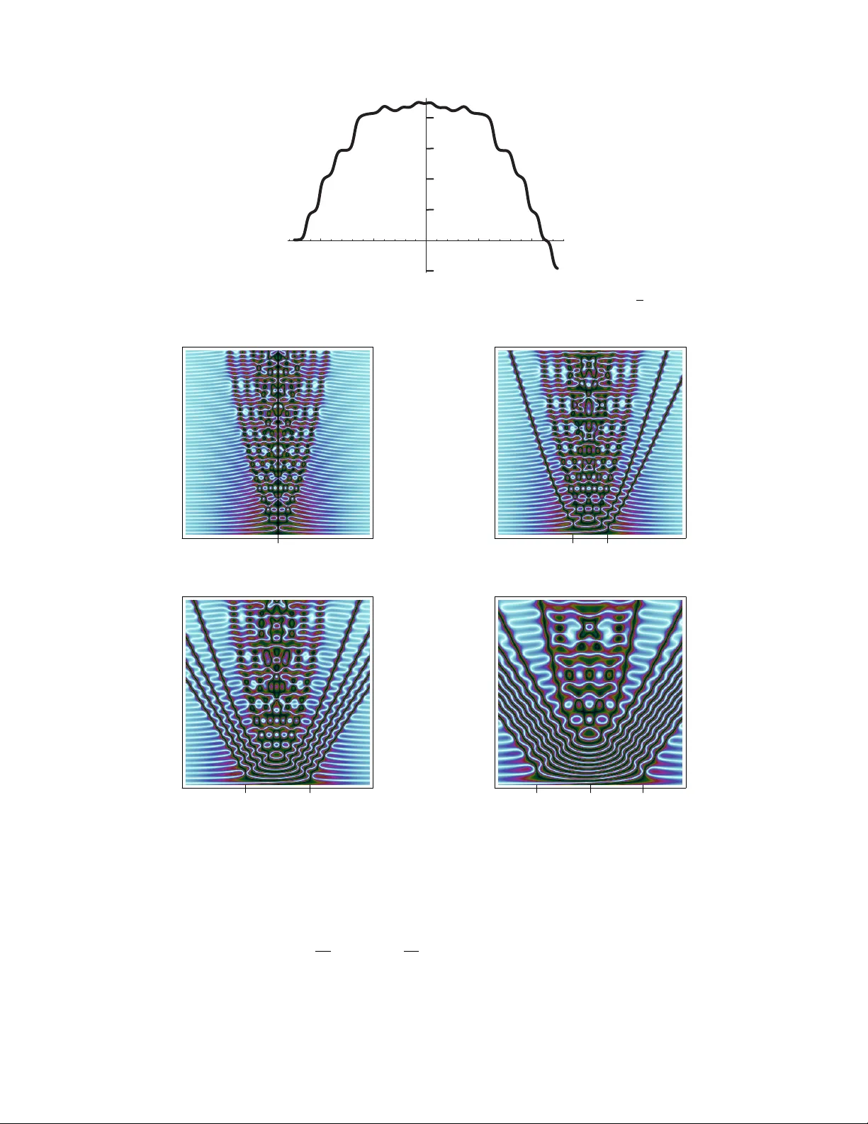
EXA CT SOLUTIONS OF SEMICLASSICAL NON-CHARA CTERISTIC CA UCHY PR OBLEMS F OR THE SINE-GORDON EQUA TION ROBER T BUCKINGHAM AND PETER D. MILLER Abstract. The use of the sine-Gordon equation as a mo del of magnetic ﬂux propagation in Josephson junctions motiv ates studying the initial-v alue problem for this equation in the semiclassical limit in whic h the dispersion parameter ε tends to zero. Assuming natural initial data having the proﬁle of a mo ving − 2 π kink at time zero, we analytically calculate the scattering data of this completely in tegrable Cauc hy problem for all ε > 0 suﬃciently small, and further we inv ert the scattering transform to calculate the solution for a sequence of arbitrarily small ε . This sequence of exact solutions is analogous to that of the well-kno wn N -soliton (or higher-order soliton) solutions of the fo cusing nonlinear Schr¨ odinger equation. Plots of exact solutions for small ε rev eal certain features that emerge in the semiclassical limit. F or example, in the limit  → 0 one observ es the appearance of nonlinear caustics, i.e. curves in space-time that are independent of ε but v ary with the initial data and that separate regions in which the solution is exp ected to hav e diﬀerent num b ers of nonlinear phases. In the app endices w e giv e a self contained accoun t of the Cauc h y problem from the p erspectives of b oth inv erse scattering and classical analysis (Picard iteration). Speciﬁcally , App endix A con tains a complete formulation of the in v erse-scattering method for generic L 1 -Sobolev initial data, and App endix B establishes the well-posedness for L p -Sobolev initial data (which in particular completely justiﬁes the in verse-scattering analysis in Appendix A). 1. Introduction The sine-Gordon equation (1) ε 2 u tt − ε 2 u xx + sin( u ) = 0 describ es a broad arra y of physical and mathematical phenomena. The partial diﬀerential equation (1) may b e regarded as the con tinuum limit of a chain of p endula sub ject to an external (gra vity) force and coupled to their nearest neighbors via Ho ok e’s la w. In nonlinear optics, the sine-Gordon equation is a sp ecial case of the Maxwell-Bloch equations and describ es self-induced transparency in the sharp-line limit [16]. In biology , the sine-Gordon equation models transcription and denaturation in DNA molecules [18]. B¨ ac klund sho w ed a corresp ondence b et w een solutions of the sine-Gordon equation and surfaces of constan t negative curv ature [9]. In solid-state physics, the sine-Gordon equation mo dels idealized magnetic ﬂux propagation along the insulating barrier b etw een t w o sup erconductors in a Josephson junction . Here the length ` 0 of the transmission line corresp onds to a length of 1 in terms of the dimensionless co ordinate x measuring distance along the junction. Let L b e the inductance p er unit length and C b e the capacitance p er unit length. Then v := ( LC ) − 1 / 2 is the typical v elo cit y parameter, and the macroscopic time scale t measures one dimensionless unit when ` 0 /v seconds ha v e passed. The parameter ε is the ratio of the Josephson length ` J to the transmission line length ` 0 . The Josephson length ` J is in turn prop ortional to Φ 1 / 2 0 , where Φ 0 := h/ (2 ε ) ≈ 2 . 064 × 10 − 15 V sec is the quantum unit of magnetic ﬂux. Laboratory exp erimen ts by Scott, Ch u, and Reible [20] analyzed ﬂux propagation in Josephson junctions of length ` 0 = 35 cm for which ` J w as appro ximately 10 − 4 to 10 − 3 m. Therefore, in these exp eriments, ε := ` J /` 0 ≈ 0 . 0005. The p erio d of a signal input to the transmission line in these exp erimen ts was typically on the order of 10 − 9 seconds, which is approximately one dimensionless time unit on the t -scale. T ogether with ε b eing small, this motiv ates the study of the semiclassic al (or zero-disp ersion) limit as ε ↓ 0. F or analytical conv enience w e c ho ose to study the Cauch y initial-v alue problem on the real line x ∈ R . F ormulating a semiclassic al Cauchy pr oblem means ﬁxing functions f and g indep enden t of ε , and then, for all ε > 0 suﬃciently small, p osing the Cauch y problem for (1) with initial data of the form u ( x, 0; ε ) = f ( x ), εu t ( x, 0; ε ) = g ( x ). See Appendix B for an accoun t of the w ell-posedness theory of this Cauc hy problem for ε > 0 ﬁxed. Solving the semiclassical Cauc h y 1 problem means obtaining the one-parameter family of solutions u ( x, t ; ε ). W e are usually most interested in the asymptotic b eha vior of the solution as ε ↓ 0. In this pap er, we consider the sine-Gordon equation (1) for all ε > 0 suﬃciently small with the initial condition (2) sin  f 2  := sec h( x ) , cos  f 2  := tanh( x ) , g := 2 µ sech( x ) , x ∈ R where µ ∈ R is a parameter. W e refer to the solution of the Cauc h y problem as u ( x, t ; ε, µ ). The top olo gic al char ge (or winding n umber) of solutions satisfying (2) is a constan t of motion given by (3) w [ u ] := 1 2 π Z + ∞ −∞ u x dx = − 1 . F rom one p oint of view, the initial data (2) are natural to study , b ecause u ( x, t ; p µ 2 + 1 , µ ) is an exact mathematical antikink solution of the sine-Gordon equation explicitly given by cos( u ( x, t ; p µ 2 + 1 , µ )) = 1 − 2 sech 2  1 εw ( x − v t )  , sin( u ( x, t ; p µ 2 + 1 , µ )) = 2 sech  1 εw ( x − v t )  tanh  1 εw ( x − v t )  (4) with velocity v and width parameter w giv en by (5) v = 1 µ 2 + 1 − µ p µ 2 + 1 − 1 , w = − 1 2 p 1 − v 2 . F rom these formulae w e see that u is a tra v eling w av e with v elo city v b ounded by 1 (the light sp eed), demonstrating the hyperb olicit y of the sine-Gordon equation. This solution admits a natural relativistic in terpretation since the relationship betw een v and w corresponds to Loren tz con traction in sp ecial relativit y . F or ε 6 = p µ 2 + 1, the initial data (2) no longer corresponds to simply one soliton, but in general excites a nonlinear sup erposition of kinks, an tikinks, breathers, and radiation. It is interesting to observ e that the initial data (2) satisﬁes the advection equation u t + vu x = 0 with constant velocity v = µ/ε . In this sense, we ma y consider the initial data as b eing in uniform motion to the right with v elocity v . Note, ho wev er, that if µ 6 = 0, then for ε > 0 suﬃcien tly small, the v elo cit y v of the initial data exceeds the constrain t | v | ≤ 1 imp osed by the hyperb olic nature of the sine-Gordon equation (1). In this situation, one migh t exp ect the sine-Gordon equation to regularize the sup erluminal velocity of the initial data for t > 0 by some kind of catastrophic eﬀect that destroys the proﬁle of the initial data. In fact, we will show (see ﬁgures 6 and 8) that the regularization of the v elo cit y takes place via the emission of a large n um b er (inv ersely prop ortional to ε ) of kink-an tikink pairs. The family of solutions corresp onding to the initial data (2) ma y b e view ed as an analogue for the sine-Gordon equation of the N -soliton (or higher-order soliton) solution to the cubic fo cusing nonlinear Sc hr¨ odinger (NLS) equation (6) iq t + 1 2 q xx + | q | 2 q = 0 . Satsuma and Y a jima [19] found that with initial data q ( x, 0; N )= N sec h( x ) the scattering data relev ant for the fo cusing NLS equation can b e found in closed form for any N ∈ R . F urthermore, if N ∈ Z then the scattering data are reﬂectionless and so the solution q ( x, t ; N ) can b e found more-or-less explicitly . In [17] it w as noted that, with ε = c/ N and τ = N t/c , the function φ ( x, τ ; ε ) = cq ( x, t ; N ) / N satisﬁes the initial-v alue problem (7) iεφ τ + ε 2 2 φ xx + | φ | 2 φ = 0 , φ ( x, 0; ε ) = c sech( x ) . The functions φ ( x, τ ; ε ) therefore solv e a semiclassical Cauch y problem since φ ( x, 0; ε ) is indep endent of ε . Numerical reconstruction of the in v erse-scattering solution for ε = ε N = c/ N , N = 1 , 2 , 3 , . . . in [17] rev ealed a spatio-temporal pattern for φ emerging as ε ↓ 0 consisting of a ﬁxed macrostructure with nonline ar c austics (phase transition b oundaries or breaking curves) separating regions of the space-time plane consisting of oscillations of diﬀerent lo cal genus (num b er of nonlinear phases). At least tw o caustic curv es app ear in the dynamics (a primary c austic t = t 1 ( x ) and a se c ondary c austic t = t 2 ( x ) > t 1 ( x )). The semiclassical 2 asymptotics for times t up to and just b ey ond the primary caustic were obtained in [12] and these results w ere extended to times t just b eyond the secondary caustic (requiring a substantial mo diﬁcation of the metho d that captures the primary caustic) in [15]. In a related result, T ovbis and V enakides [21] generalized the calculation of Satsuma and Y a jima by computing the scattering data asso ciated with the semiclassically- scaled fo cusing NLS equation (7) explicitly for all suﬃciently small ε > 0 when the initial data is given in the form (8) φ ( x, 0; µ ) = A ( x ) e iS ( x ) /ε , S 0 ( x ) = − µ tanh( x ) , A = c sech( x ) . Subsequen tly , the Cauch y problem for (7) with this initial data has been studied b y T o vbis, V enakides, and Zhou [22, 23]. In this pap er, we presen t a calculation of the scattering data for (1)–(2) analogous to the w ork in [19] and [21], and w e also presen t an explicit computation of u ( x, t ; ε, µ ) as ε ↓ 0 analogous to [17]. The asymptotic analysis of the semiclassical Cauc h y problem for sine-Gordon corresp onding to the w ork in [12, 15, 22, 23] will b e carried out in a later work. The sine-Gordon equation (1) is an integrable system, p ossessing a Lax pair (see (123) and (124)) and admitting all the b eneﬁts thereof, including the existence of inv erse-scattering transforms for solving Cauc hy problems in v arious co ordinate systems. W e consider the Cauch y problem in lab oratory co ordinates and we use the Riemann-Hilbert form ulation of inv erse scattering. F or the sine-Gordon equation in char- acteristic coordinates, the inv erse-scattering metho d was ﬁrst given in [1] and [25]. The in v erse-scattering metho d corresponding to the (nonc haracteristic) Cauc h y problem for the sine-Gordon equation in lab oratory co ordinates was work ed out by Kaup [13]. An accoun t of the Riemann-Hilbert method for carrying out the in verse step in lab oratory co ordinates can b e found in the text of F addeev and T akh ta jan [8], and further dev elopments to the theory were made b y Zhou [26] and Cheng et al. [4]. In our paper, w e add to this lit- erature by giving in Appendix A a complete description of the Riemann-Hilbert form ulation of the solution of the Cauc h y problem in lab oratory co ordinates assuming that at each instan t of time the solution u has L 1 -Sob olev regularit y . That the sine-Gordon equation (1) preserv es this degree of regularity if it is present at t = 0 is established b y indep endent arguments in App endix B. Brieﬂy , the in verse-scattering method proceeds as follows. Cauch y data for the sine-Gordon equation c haracterize a set of scattering data, which consist of the r eﬂe ction c o eﬃcient ρ : R → C , the eigenvalues { z n } , and the mo diﬁe d pr op ortionality c onstants { c n } . The scattering data are used to formulate a Riemann- Hilb ert problem with an explicit, elementary dependence on x and t . While it is not in general p ossible to solv e a Riemann-Hilbert problem in closed form, for r eﬂe ctionless Cauc h y data (i.e. for which ρ ( z ) ≡ 0) the Riemann-Hilb ert problem can b e reduced to the solution of a system of linear algebraic equations. In Section 2, we explicitly calculate the scattering data corresponding to viewing the initial data (2) as a kind of potential in the linear scattering problem (123) asso ciated with the Cauch y problem for the sine-Gordon equation (1). Our analysis will b e v alid for all µ ∈ R and ε > 0 suﬃcien tly small. F urthermore, w e sho w that if ε lies in the sequence (9) ε = ε N ( µ ) := p µ 2 + 1 2 N + 1 , N ∈ Z + := { 0 , 1 , 2 , . . . } (note that this sequence conv erges to zero as N → ∞ ), then the scattering data are reﬂectionless ultimately implying via inv erse-scattering theory that u can be computed explicitly (that is, u can b e expressed b y a ﬁnite num b er of arithmetic operations). The inv erse step is carried out for ε in the sequence (9) corresp onding to reﬂectionless initial data in Section 3, where cos( u ) and sin( u ) are extracted b y considering an appropriate limit of the solution to the Riemann-Hilb ert problem. As ε ↓ 0 through this sequence, a pattern emerges in whic h u consists of modulated wa ve trains of w av e n umber and frequency inv ersely prop ortional to ε with one or more nonlinear phases. The spatio-temp oral scale of the mo dulation is ﬁxed as ε ↓ 0. Regions of space-time containing wa v es with diﬀeren t num b ers of nonlinear phases are separated b y nonlinear caustics that are independent of ε for ﬁxed µ . See ﬁgures 5, 6, and 8 for plots of cos( u ) exhibiting these features for v arious v alues of ε and µ . At a qualitativ e lev el, these features resem ble those observed for solutions of the semiclassical Cauch y problem for the fo cusing NLS equation. Section 4 discusses the limitations inheren t in an approach to the semiclassical limit based upon calculations of complexit y and sensitivity increasing with N ∼ ε − 1 , and explores p ossible extensions. 3 R emark 1 . Under the scalings x = εX and t = εT and the choice ε = ε N ( µ ) (see (9)), equations (1) and (2) b ecome (10) U T T − U X X + sin( U ) = 0 , sin  1 2 U ( X , 0; N , µ )  = sec h ( ε N ( µ ) X ) , cos  1 2 U ( X , 0; N , µ )  = tanh ( ε N ( µ ) X ) , U T ( X, 0; N , µ ) = 2 µ sec h ( ε N ( µ ) X ) , (11) where U ( X , T ; N , µ ) = u ( x, t ; ε, µ ). This is a ﬁxed-disp ersion Cauch y problem with a sequence of diﬀerent initial conditions dep ending on N , just as in the problem for the NLS equation studied b y Satsuma and Y a jima. The initial conditions all ha v e topological charge w [ U ] = − 1 but U ( X, 0; N , µ ) and U T ( X, 0; N , µ ) b ecome more dilated in X (slo wly-v arying) as N increases. Therefore, an alternate wa y of viewing our result is that we can ﬁnd exact solutions to the ﬁxed-disp ersion initial-v alue problem (10)–(11) for N ∈ Z + . As an example of an explicit solution of (10) obtained in this wa y , when N = 1 and µ = 0 we hav e (12) cos( U ( X , T ; 1 , 0)) = 1 − 2 n ( X, T ) 2 d ( X, T ) 2 , where n ( X, T ) := 11 + cos 4 √ 2 3 T ! + 8 cosh  2 3 X  + 4 cos 2 √ 2 3 T !  2 cosh  2 3 X  + cosh  4 3 X  d ( X, T ) := 4 " 2 + 3 cos 2 √ 2 3 T !# cosh  1 3 X  + " 9 + cos 4 √ 2 3 T !# cosh( X ) + 2 cosh  5 3 X  . (13) The fo cusing NLS equation (6) admits a scaling symmetry in which scaling the independent v ariable x is equiv alent to scaling the dep endent v ariable (amplitude) q and the time t . Th us, the N -soliton (or higher- order soliton) solutions of the fo cusing NLS equation that w ere originally obtained by Satsuma and Y a jima [19] by considering a ﬁxed-width pulse with v ariable amplitude can just as easily b e viewed as a ﬁxed- amplitude pulse with v ariable width. F rom the p oin t of view of semiclassical asymptotics, dilation in x is the more natural in terpretation of the higher-order solitons as the presence of the parameter ε in (7) amounts to rescaling x and t , and th us the v ariable width of the pulse is absorbed into the semiclassical parameter ε as in [17, 12]. Of course, the sine-Gordon equation do es not admit the amplitude/dilation symmetry enjoy ed b y the focusing NLS equation, so we are not free to in terpret the family of exact solutions w e obtain in this pap er in terms of scaling of amplitude. It seems that p erhaps a more generally fruitful approac h to seeking analogues of the higher-order soliton in other integrable systems is to consider pulse width dilation as being more fundamental than amplitude dilation. As more evidence of the utility of this approach (b eyond the sine-Gordon example), the mo diﬁed NLS equation (which includes an additional term in (6) that breaks the scaling symmetry needed to exc hange amplitude for width) do es not hav e higher-order solitons in the sense of Satsuma and Y a jima, but it do es ha v e exact solutions corresp onding to arbitrarily width-dilated pulses that are useful in semiclassical analysis [5]. R emark 2 . In c haracteristic or light-cone co ordinates χ and τ deﬁned by x = χ + τ and t = χ − τ , the sine-Gordon equation (1) is ε 2 v χτ = sin( v ), where v ( χ, τ ; ε ) = u ( x, t ; ε ). The asso ciated χ evolution equation in the Lax pair is the Zakharo v-Shabat eigenv alue equation, which is the same eigenv alue equation as for the fo cusing NLS equation [24]. Thus it is p ossible to solv e a semiclassical characteristic Cauc h y problem with sp ecial initial data v ( χ, 0; ε ) = c sech( χ ) using the Satsuma-Y a jima higher-order soliton solution. How ev er, in man y applications (as in Josephson junction theory), the correct problem is the non-characteristic Cauc h y problem with tw o indep enden t initial conditions: u ( x, 0; ε ) = f ( x ), εu t ( x, 0; ε ) = g ( x ). The Satsuma-Y a jima solution to the semiclassical problem p osed along a c haracteristic τ = 0 or x = t will ha ve a v ery complicated and unwieldy form and an undesired dep endence on ε up on restriction to t = 0, and therefore is probably not relev an t to the non-c haracteristic semiclassical Cauch y problem w e wish to consider. On notation . As will b e explained in detail in Section 2 and App endix A, w e will use three diﬀerent gauges for the eigenv alue problem. Ob jects asso ciated with the inﬁnity gauge will b e denoted b y an ov erline ( J ). Ob jects asso ciated with the zer o gauge will b e denoted b y an underline ( J ). Finally , ob jects asso ciated with 4 the symmetric gauge will not hav e a bar ( J ). The complex conjugate of a is denoted b y a ∗ . W e use the notation f ( a, b ; c ) to emphasize that c is a parameter. The dep endence on parameters may b e suppressed by writing f ( a, b ) in place of f ( a, b ; c ). W e also make frequen t use of the standard P auli matrices deﬁned as (14) σ 1 :=  0 1 1 0  , σ 2 :=  0 − i i 0  , σ 3 :=  1 0 0 − 1  . V ectors will be denoted b y b old lo wer-case letters and matrices b y b old upper-case letters, with the exception of the Pauli matrices. The transp ose of a vector v is denoted by v T , and the conjugate-transp ose of a matrix A is denoted b y A † . Finally , χ S ( · ) denotes the c haracteristic function (indicator function) of a set S , that is χ S ( x ) = 1 if x ∈ S and χ S ( x ) = 0 otherwise. 2. Sca ttering Theor y for the Special Initial Da t a The quan tities z ± z − 1 app ear throughout the scattering and in verse-scattering theory of the sine- Gordon equation (1), and so for con venience w e deﬁne (15) D ( z ) := 1 4  z + 1 z  , E ( z ) := 1 4  z − 1 z  . Fix the initial condition (2). T o ﬁnd the scattering data it is necessary to solv e the following generalized eigen v alue problem for J ( x ; z , t, ε, µ ) (see, for example, [13]): (16) 4 iε J x =  4 E + z − 1 (1 − cos( u )) − z − 1 sin( u ) − iε ( u x + u t ) − z − 1 sin( u ) + iε ( u x + u t ) − 4 E − z − 1 (1 − cos( u ))  J . This formulation of the eigenv alue problem is useful in the study of solutions J when z is b ounded aw ay from 0 (see [13] and Prop osition A.1 b elo w), and for this reason, w e say that (16) is written in the inﬁnity gauge . The use of alternate gauges pro v es to b e b eneﬁcial. F or example, the gauge transformation (139) (see App endix A) casts the eigen v alue problem (16) into an alternate form that is useful in the analysis of solutions corresponding to bounded z , and in particular near z = 0 (see [13] and Proposition A.2). Therefore, w e refer to the co ordinate system arrived at via the transformation (139) as the zer o gauge . While the inﬁnity gauge and the zero gauge are useful in the analysis of the scattering problem required to form ulate an in verse- scattering theory , to calculate the scattering data corresp onding to (2) we found it to b e useful to introduce a gauge transformation that symmetrizes the appearance of z and z − 1 in the eigenv alue problem and at the same time also remov es the function u x from the co eﬃcients. It is in this third, symmetric gauge that it is easiest to see the eigen v alue problem is in fact h ypergeometric for the initial data (2). Once it is clear from w orking in the symmetric gauge that the eigen v alue problem has exactly three regular singular points, it is p ossible to use the theory of Euler transforms to analyze the asymptotic b ehavior of the Jost solutions and th us obtain the scattering data. 2.1. T ransformation to a h yp ergeometric equation. The ﬁrst step in transforming (16) in to a hyper- geometric equation is to introduce an appropriate gauge transformation. If J satisﬁes equation (16), then the inv ertible transformation (ha ving an interpretation as a rotation at each x b y an angle − u/ 4) (17) J ( x ; z , t, ε, µ ) = AJ :=     cos  u 4  sin  u 4  − sin  u 4  cos  u 4      J yields a solution J of the eigen v alue problem written in the symmetric gauge : (18) 4 iε J x =     4 E cos  u 2  − 4 D sin  u 2  − iεu t − 4 D sin  u 2  + iεu t − 4 E cos  u 2      J . W ritten in this form 1 , the eigenv alue problem app ears similar to one used by F addeev and T akhta jan (see [8] part 2, c hapter 2, equation 4.1). The Jost solutions J ± in the symmetric gauge are deﬁned to be the 1 The absence of u x in the symmetrized form (18) of the eigen value problem pro vides an alternate framew ork in which to consider discontin uous initial data without the use of delta functions ( cf. [11]). 5 fundamen tal solution matrices of the linear problem (18) for r e al v alues of z , normalized b y the conditions J − =  e iE x/ε 0 0 − e − iE x/ε  + o (1) as x → −∞ for z ∈ R , J + =  e − iE x/ε 0 0 e iE x/ε  + o (1) as x → + ∞ for z ∈ R . (19) W e denote the columns in this wa y: J ± =: [ j ± 1 , j ± 2 ]. They are related to the Jost solutions for the inﬁnity gauge (see (125)) by (20) j − 1 = Aj − 2 , j − 2 = Aj − 1 , j + 1 = Aj + 1 , j + 2 = Aj + 2 . F or the choice of initial condition (2), the eigen v alue equation (18) takes the form (21) 2 iε J x =  2 E tanh( x ) ( − 2 D − iµ ) sech( x ) ( − 2 D + iµ ) sech( x ) − 2 E tanh( x )  J . With the c hange of indep enden t v ariable (22) y = tanh( x ) , the eigenv alue problem (21) becomes (23) 2 iε (1 − y 2 ) J y =  2 E y ( − 2 D − iµ ) (1 − y 2 ) 1 / 2 ( − 2 D + iµ ) (1 − y 2 ) 1 / 2 − 2 E y  J . Here − 1 < y < 1 and the p ositiv e square root is chosen. There are t w o wa ys to eliminate the square ro ots in the co eﬃcien t matrix. The ﬁrst is to introduce the linear transformation (24) j + 1 =  1 0 0 (1 − y 2 ) 1 / 2  g , whic h results in a diﬀerential equation satisﬁed b y g ( y ; z , ε, µ ): (25) 2 iε (1 − y 2 ) g y =  2 E y ( − 2 D − iµ ) (1 − y 2 ) − 2 D + iµ ( − 2 E + 2 iε ) y  g . This equation has exactly three regular singular p oin ts y ∈ {− 1 , 1 , ∞} and can b e written in hypergeometric form. W e will use (25) to ﬁnd expressions for j + 1 and j − 1 . R emark . If w e had taken (16) instead of (18) as our starting p oin t and follow ed analogous steps, namely (i) substitution of the initial data using double-angle formulae, (ii) the indep enden t v ariable transformation y = tanh( x ), and (iii) the use of the gauge transformation (24) to reduce the problem to rational form, w e w ould ha ve arrived at (26) 2 iε (1 − y 2 ) g y =  2 E + z − 1 (1 − y 2 ) − z − 1 (1 − y 2 ) y + iε (1 − y 2 ) − z − 1 y − iε − 2 E − z − 1 (1 − y 2 ) + 2 iεy  g instead of (25). Let v = y − 1 . Then near v = 0, (26) has the leading-order form g v = O ( v − 3 ) · g , whereas (25) has the leading-order form g v = O ( v − 2 ) · g . After some calculation it is p ossible to see that the metho d of F rob enius still applies to (26) near v = 0 even with the additional growth at y = ∞ due to sp ecial iden tities holding among the entries of the matrix co eﬃcien ts of the leading-order terms. Ho w ever, the lo cal (F rob enius) analysis of (25) is more straightforw ard with only a double p ole at v = 0. Later we will also see that it is more diﬃcult to obtain integral representations for solutions of (26) than for (25). An alternative to the linear transformation (24) is (27) j + 2 =  1 0 0 (1 − y 2 ) − 1 / 2  h , whic h after substitution in to (23) yields the diﬀerential equation for h ( y ; z , ε, µ ): (28) 2 iε (1 − y 2 ) h y =  2 E y − 2 D − iµ ( − 2 D + iµ ) (1 − y 2 ) ( − 2 E − 2 iε ) y  h . 6 This equation also has exactly three regular singular p oints y ∈ {− 1 , 1 , ∞} . It will b e used to ﬁnd expressions for j + 2 and j − 2 . 2.2. In tegral representations for Jost solutions. W e no w use the theory of Euler transforms [10] to deriv e in tegral represen tations for the four Jost solutions, starting with j + 1 and j − 1 . Deﬁne (29) γ = γ ( µ ) := p µ 2 + 1 . Prop osition 2.1. Cho ose the princip al br anches of the functions ( s ± 1) − 1 / 2+ γ / 2 ε with br anch cuts on the r e al s -axis fr om ∓ 1 to −∞ . Also cho ose the princip al br anch of ( s − y ) − iE /ε − γ / 2 ε − 1 with br anch cut on the r e al s -axis fr om y to −∞ . T ake Σ + to b e a close d c ontour in the s -plane p assing thr ough the br anch p oint s = − 1 and encir cling s = 1 onc e in the c ounter clo ckwise dir e ction (se e ﬁgur e 1(a)). Then, for z ∈ R \{ 0 } , s = y s = 1 s = − 1 Σ + (a) The contour Σ + . Σ − s = y s = − 1 s = 1 (b) The contour Σ − . Figure 1. The in tegration con tours and branch cuts for the Jost functions. j + 1 =: [ J + 11 , J + 21 ] T is given by (30) J + 11 = C 1 (1 − y 2 ) iE / 2 ε Z Σ + ( s − 1) − 1 / 2+ γ / 2 ε ( s + 1) − 1 / 2+ γ / 2 ε ( s − y ) − iE /ε − γ / 2 ε ds (31) J + 21 = C 1 (1 − y 2 ) iE / 2 ε +1 / 2  z − ( γ + µ ) i z + ( γ + µ ) i  Z Σ + ( s − 1) − 1 / 2+ γ / 2 ε ( s + 1) − 1 / 2+ γ / 2 ε ( s − y ) − iE /ε − γ / 2 ε − 1 ds with (32) C 1 = C 1 ( z , ε, µ ) := Γ  1 2 + iE ε  Γ  1 + γ 2 ε − iE ε  2 1+ γ / 2 ε iπ Γ  1 2 + γ 2 ε  . Pr o of. W e b egin by computing the F rob enius exponents of (25). Assume that, for some n um ber p + ∈ C , g has a F rob enius series ab out y = 1 of the form (33) g ( y ) = ∞ X n =0 g + n (1 − y ) p + + n for some v ector-v alued co eﬃcien ts g + n . Substituting this series in to equation (25) and considering the leading- order terms immediately gives the (indicial) eigenv alue equation (34) − 4 iεp + g + 0 =  2 E 0 − 2 D + iµ − 2 E + 2 iε  g + 0 . Therefore, the F rob enius exp onents at y = 1 are (35) p + = iE 2 ε , − iE 2 ε − 1 2 . Similarly , substituting a series of the form (36) g ( y ) = ∞ X n =0 g − n (1 + y ) p − + n in to equation (25) and considering the leading-order terms sho ws that the F rob enius exp onen ts at y = − 1 are exactly the same: (37) p − = iE 2 ε , − iE 2 ε − 1 2 . 7 W e no w shift t w o of the exp onents to zero via the substitution (38) g ( y ) = (1 − y 2 ) iE / 2 ε f ( y ) . It follows that f ( y ; z , ε, µ ) satisﬁes the diﬀeren tial equation (39) 2 iε (1 − y 2 ) f y =  0 ( − 2 D − iµ ) (1 − y 2 ) − 2 D + iµ ( − 4 E + 2 iε ) y  f . W e attempt to express f =: [ f 1 , f 2 ] T as (40) f 1 ( y ) = Z Σ + F 1 ( s )( s − y ) α ds, f 2 ( y ) = Z Σ + F 2 ( s )( s − y ) β ds where the Euler transforms F 1 , 2 ( s ; z , ε, µ ) and the constant exp onen ts α = α ( z , ε, µ ) and β = β ( z , ε, µ ) remain to be chosen. Substituting the express ions (40) into the system (39) shows that the ﬁrst equation 2 iεf 1 y = ( − 2 D − iµ ) f 2 can b e easily solved by c ho osing (41) F 2 ( s ) = 2 iεα (2 D + iµ ) F 1 ( s ) and β = α − 1 . R emark . The fact that there is suc h a simple relationship b etw een F 1 and F 2 is related to the fact that f 2 could b e easily eliminated to write a second-order diﬀeren tial equation for f 1 that is essentially the Gauss h yp ergeometric equation. On the other hand, if w e had work ed from the beginning in the inﬁnity gauge, the elimination of f 2 using the ﬁrst ro w of (26) would hav e resulted in a second-order equation that is not ob viously of hypergeometric form. This, in turn, w ould lead to further complications in the follo wing analysis leading from (43) to (49). It remains to satisfy the second equation of the system (39): (42) 2 iε (1 − y 2 ) f 2 y = ( − 2 D + iµ ) f 1 + ( − 4 E + 2 iε ) y f 2 . W riting y = s − ( s − y ) and 1 − y 2 = (1 − s 2 ) + 2 s ( s − y ) − ( s − y ) 2 and using equations (41) giv es − 2 iε 2 α ( α − 1) (2 D + iµ ) Z Σ + F 1 ( s )  (1 − s 2 )( s − y ) α − 2 + 2 s ( s − y ) α − 1 − ( s − y ) α  ds =  iD + µ 2  Z Σ + F 1 ( s )( s − y ) α ds (43) + (2 iE + ε ) 2 iεα (2 D + iµ ) Z Σ + F 1 ( s )  s ( s − y ) α − 1 − ( s − y ) α  ds. If we now choose α to satisfy the quadratic equation (44) 2 iε 2 α ( α − 1) (2 D + iµ ) =  iD + µ 2  − (2 iE + ε ) 2 iεα (2 D + iµ ) then the ( s − y ) α terms will cancel in equation (43). Sp eciﬁcally , w e choose (45) α = − iE ε − γ 2 ε . Using integration by parts to eliminate the ( s − y ) α − 2 term yields − ε Z Σ + d ds  F 1 ( s )(1 − s 2 )  ( s − y ) α − 1 ds + 2 ε ( α − 1) Z Σ + F 1 ( s ) s ( s − y ) α − 1 ds = ( − 2 iE − ε ) Z Σ + F 1 ( s ) s ( s − y ) α − 1 ds. (46) Setting the in tegrands equal and using equation (45) for α gives the ﬁrst-order linear diﬀe ren tial equation (47) ε (1 − s 2 ) d ds F 1 ( s ) = ( ε − γ ) sF 1 ( s ) or (48) d ds log F 1 ( s ) =  γ 2 ε − 1 2  1 s − 1 +  γ 2 ε − 1 2  1 s + 1 8 for F 1 ( s ). The general solution (49) F 1 ( s ) = C 1 ( s − 1) − 1 / 2+ γ / 2 ε ( s + 1) − 1 / 2+ γ / 2 ε , where C 1 is an in tegration constan t, giv es equations (30) and (31) up to the c hoice of the constan t C 1 . The constant C 1 is to b e chosen so that j + 1 is normalized as required in equation (19). Consider equation (30) for J + 11 as y → 1. Now for s ∈ Σ + , (50)    ( s − 1) − 1 / 2+ γ / 2 ε ( s + 1) − 1 / 2+ γ / 2 ε ( s − y ) − iE /ε − γ / 2 ε    ≤    ( s − 1) − 1 / 2+ γ / 2 ε ( s − y ) − iE /ε − γ / 2 ε    | s + 1 | − 1 / 2+ γ / 2 ε ≤ K | s + 1 | − 1 / 2+ γ / 2 ε for some constant K > 0, as Σ + is bounded aw ay from s = y and s = 1. Since γ / 2 ε > 0, the function | s + 1 | − 1 / 2+ γ / 2 ε is integrable on Σ + . Therefore, b y Leb esgue’s dominated conv ergence theorem, (51) J + 11 = C 1 (1 − y 2 ) iE / 2 ε  Z Σ + ( s + 1) − 1 / 2+ γ / 2 ε ( s − 1) − iE /ε − 1 / 2 ds + o (1)  as y → 1 . The in tegrand is in tegrable at s = 1, so w e can collapse Σ + to the upp er and low er edges of the branc h cut [ − 1 , 1], yielding (52) Z Σ + ( s + 1) − 1 / 2+ γ / 2 ε ( s − 1) − iE /ε − 1 / 2 ds =2 i sin  π  1 2 + iE ε  Z 1 − 1 ( s + 1) − 1 / 2+ γ / 2 ε (1 − s ) − 1 / 2 − iE /ε ds = 2 iπ Γ  1 2 + iE ε  Γ  1 2 − iE ε  Z 1 − 1 ( s + 1) − 1 / 2+ γ / 2 ε (1 − s ) − 1 / 2 − iE /ε ds. In the last step w e used the reﬂection identit y (53) sin( π z ) = π Γ( z )Γ(1 − z ) . The remaining in tegral is a b eta in tegral, whic h may b e expressed in terms of gamma functions. Indeed, making the c hange of v ariables s = 2 w − 1 giv es Z 1 − 1 ( s + 1) − 1 / 2+ γ / 2 ε (1 − s ) − 1 / 2 − iE /ε ds = 2 γ / 2 ε − iE /ε Z 1 0 w − 1 / 2+ γ / 2 ε (1 − w ) − 1 / 2 − iE /ε dw = 2 γ / 2 ε − iE /ε Γ  1 2 + γ 2 ε  Γ  1 2 − iE ε  Γ  1 + γ 2 ε − iE ε  (54) using the iden tity (55) Z 1 0 w a − 1 (1 − w ) b − 1 dw = Γ( a )Γ( b ) Γ( a + b ) v alid for < ( a ) , < ( b ) > 0. Also note that, as y → 1, (56) 1 − y 2 = sec h 2 ( x ) = 2 2 e − 2 x (1 + o (1)) . Therefore, as x → + ∞ , (57) J + 11 = C 1 e − iE x/ε " 2 1+ γ / 2 ε iπ Γ  1 2 + γ 2 ε  Γ  1 2 + iE ε  Γ  1 + γ 2 ε − iE ε  + o (1) # . Comparing equations (19) and (57) gives the expression (32) for the constan t C 1 .  Prop osition 2.2. Cho ose the princip al br anches of the functions ( ± 1 − s ) − 1 / 2+ γ / 2 ε with br anch cuts on the r e al s -axis fr om ± 1 to + ∞ . Also cho ose the princip al br anch of ( y − s ) − iE /ε − γ / 2 ε − 1 with br anch cut on the r e al s -axis fr om y to + ∞ . T ake Σ − to b e a close d c ontour in the s -plane p assing thr ough the br anch p oint 9 s = 1 and encir cling s = − 1 onc e in the c ounter clo ckwise dir e ction (se e ﬁgur e 1(b)). Then, for z ∈ R \{ 0 } , j − 1 =: [ J − 11 , J − 21 ] T is given by (58) J − 11 = C 1 (1 − y 2 ) iE / 2 ε Z Σ − ( − 1 − s ) − 1 / 2+ γ / 2 ε (1 − s ) − 1 / 2+ γ / 2 ε ( y − s ) − iE /ε − γ / 2 ε ds (59) J − 21 = − C 1 (1 − y 2 ) iE / 2 ε +1 / 2  z − ( γ + µ ) i z + ( γ + µ ) i  Z Σ − ( − 1 − s ) − 1 / 2+ γ / 2 ε (1 − s ) − 1 / 2+ γ / 2 ε ( y − s ) − iE /ε − γ / 2 ε − 1 ds with C 1 given by e quation (32). Pr o of. The construction follo ws that of j + 1 , except with Σ − in place of Σ + , and c hoice of the solution (60) F 1 ( s ) = C 1 ( − 1 − s ) − 1 / 2+ γ / 2 ε (1 − s ) − 1 / 2+ γ / 2 ε to equation (48).  No w we use the system of diﬀeren tial equations in the form (28) resulting from the transformation (27) to ﬁnd expressions for the Jost solutions j + 2 and j − 2 . Prop osition 2.3. T ake ( s ± 1) − 1 / 2+ γ / 2 ε , ( s − y ) − iE /ε − γ / 2 ε − 1 , and Σ + as in Pr op osition 2.1. Then, for z ∈ R \{ 0 } , j + 2 =: [ J + 12 , J + 22 ] T is given by (61) J + 12 = − C 2 (1 − y 2 ) − iE / 2 ε +1 / 2  z + ( γ + µ ) i z − ( γ + µ ) i  Z Σ + ( s − 1) − 1 / 2+ γ / 2 ε ( s + 1) − 1 / 2+ γ / 2 ε ( s − y ) iE /ε − γ / 2 ε − 1 ds (62) J + 22 = C 2 (1 − y 2 ) − iE / 2 ε Z Σ + ( s − 1) − 1 / 2+ γ / 2 ε ( s + 1) − 1 / 2+ γ / 2 ε ( s − y ) iE /ε − γ / 2 ε ds with (63) C 2 = C 2 ( z , ε, µ ) := Γ  1 2 − iE ε  Γ  1 + γ 2 ε + iE ε  2 1+ γ / 2 ε iπ Γ  1 2 + γ 2 ε  . Pr o of. The F rob enius exp onents p − around y = − 1 and p + around y = 1 for h satisfying (28) are (64) p − = iE 2 ε , − iE 2 ε + 1 2 , p + = iE 2 ε , − iE 2 ε + 1 2 . Therefore, deﬁning f ( y ; z , ε, µ ) = [ f 1 ( y ; z , ε, µ ) , f 2 ( y ; z , ε, µ )] T in terms of h b y (65) h ( y ) = (1 − y 2 ) − iE / 2 ε +1 / 2 f ( y ) has the eﬀect of shifting one exp onent to zero near eac h of the p oints y = ± 1. By direct calculation, f satisﬁes (66) 2 iε (1 − y 2 ) f y =  (4 E + 2 iε ) y − 2 D − iµ ( − 2 D + iµ ) (1 − y 2 ) 0  f . Assume integral representations of the form (67) f 1 ( y ) = Z Σ + F 1 ( s )( s − y ) α ds, f 2 ( y ) = Z Σ + F 2 ( s )( s − y ) β ds. Pro ceeding as in Prop osition 2.1, w e obtain F 1 ( s ) = −  z + ( γ + µ ) i z − ( γ + µ ) i  F 2 ( s ) , F 2 ( s ) = C 2 ( s − 1) − 1 / 2+ γ / 2 ε ( s + 1) − 1 / 2+ γ / 2 ε , α = β − 1 , β = iE ε − γ 2 ε , (68) where C 2 is a constan t of integration. The constan t C 2 is c hosen so j + 2 is normalized as required in equation (19). Starting with equation (62) for J + 22 , for s ∈ Σ + w e ha ve (69)    ( s − 1) − 1 / 2+ γ / 2 ε ( s + 1) − 1 / 2+ γ / 2 ε ( s − y ) iE /ε − γ / 2 ε    ≤ K | s + 1 | − 1 / 2+ γ / 2 ε 10 for some constan t K > 0. By dominated con vergence, (70) J + 22 = C 2 (1 − y 2 ) − iE / 2 ε  Z Σ + ( s − 1) − 1 / 2+ γ / 2 ε ( s + 1) iE /ε − 1 / 2 ds + o (1)  as y → 1 . This is the same expression as equation (51) for J + 11 with C 1 and E replaced with C 2 and − E , resp ectiv ely . Therefore, as y → 1, J + 22 = C 2 e iE x/ε " 2 1+ γ / 2 ε i sin  π  1 2 − iE ε  Γ  1 2 + γ 2 ε  Γ  1 2 + iE ε  Γ  1 + γ 2 ε + iE ε  + o (1) # = C 2 e iE x/ε " 2 1+ γ / 2 ε iπ Γ  1 2 + γ 2 ε  Γ  1 2 − iE ε  Γ  1 + γ 2 ε + iE ε  + o (1) # (71) using the iden tity (53), which gives equation (63).  Prop osition 2.4. Deﬁne ( ± 1 − s ) − 1 / 2+ γ / 2 ε , ( y − s ) − iE /ε − γ / 2 ε − 1 , and Σ − as in Pr op osition 2.2. Then, for z ∈ R \{ 0 } , j − 2 =: [ J − 12 , J − 22 ] T is given by (72) J − 12 = − C 2 (1 − y 2 ) − iE / 2 ε +1 / 2  z + ( γ + µ ) i z − ( γ + µ ) i  Z Σ − ( − 1 − s ) − 1 / 2+ γ / 2 ε (1 − s ) − 1 / 2+ γ / 2 ε ( y − s ) iE /ε − γ / 2 ε − 1 ds (73) J − 22 = C 2 (1 − y 2 ) − iE / 2 ε Z Σ − ( − 1 − s ) − 1 / 2+ γ / 2 ε (1 − s ) − 1 / 2+ γ / 2 ε ( y − s ) iE /ε − γ / 2 ε ds with C 2 given by e quation (63). Pr o of. The integral representation for j − 2 is derived in the same wa y as the representation for j + 2 in Prop osition 2.3, with Σ − replacing Σ + and the c hoice F 2 ( s ) = C 2 ( − 1 − s ) − 1 / 2+ γ / 2 ε (1 − s ) − 1 / 2+ γ / 2 ε .  2.3. The scattering data. W e now use the in tegral form ulae from Section 2.3 to calculate the scattering matrix S , the eigenv alues { z n } , and (in certain special cases of in terest) the prop ortionality constants { η n } . Prop osition 2.5. The c o eﬃcient S 22 ( z ) = S 22 ( z ; ε, µ ) is given by (74) S 22 ( z ) = ( z − ( γ + µ ) i ) ( z + ( γ + µ ) i ) ·  Γ  1 2 − iE ε  2 Γ  1 − γ 2 ε − iE ε  Γ  γ 2 ε − iE ε  , z ∈ R . Pr o of. T ake z ∈ R \{ 0 } . By equations (167) and (20), (75) j + 2 = S 22 j − 1 + S 12 j − 2 . T o determine S 22 w e use (76) S 22 = det  j + 2 , j − 2  det  j − 1 , j − 2  = − lim x →−∞ det  j + 2 , j − 2  = lim x →−∞  J + 12 e − iE x/ε  . W e no w analyze J + 12 as x → −∞ . Consider the in tegral (77) I 1 ( y ; z , ε, µ ) := Z Σ + ( s − 1) − 1 / 2+ γ / 2 ε ( s + 1) − 1 / 2+ γ / 2 ε ( s − y ) iE /ε − γ / 2 ε − 1 ds. Making the substitution s = − 1 + ( y + 1) v gives I 1 = ( y + 1) iE /ε − 1 / 2 Z b Σ + ( − 2 + ( y + 1) v ) − 1 / 2+ γ / 2 ε v − 1 / 2+ γ / 2 ε ( v − 1) iE /ε − γ / 2 ε − 1 dv =: ( y + 1) iE /ε − 1 / 2 I 2 . (78) Here we tak e b Σ + to b e the counterclockwise-orien ted con tour starting at v = 0, following the semicircle in the lo wer half-plane of unit radius cen tered at v = 1 to v = 2, pro ceeding along the real axis to v = 2 / ( y + 1), coming bac k along the real axis to v = 2 along the top side of the branc h cut, and then returning to v = 0 along the semicircle in the upp er half-plane of unit radius centered at v = 1. See ﬁgure 2(a). Now for v ∈ b Σ + , (79) | − 2 + ( y + 1) v | = | y + 1 | ·     v − 2 y + 1     ≤ | y + 1 | · 2 | y + 1 | = 2 . 11 v = 0 v = 1 v = 2 y + 1 ! Σ + (a) The contour b Σ + . s = − 1 + i s = − 1 − i s = y s = 1 Σ 2+ Σ 1+ Σ 1+ (b) The contours Σ 1+ and Σ 2+ . Figure 2. The in tegration con tours used to calculate S 22 ( z ) and S 12 ( z ). The inequality ab ov e follo ws b ecause the contour b Σ + lies inside the circle of radius 2 / ( y + 1) centered at v = 2 / ( y + 1). Therefore, for v ∈ b Σ + with | v − 1 | = 1, (80)    ( − 2 + ( y + 1) v ) − 1 / 2+ γ / 2 ε v − 1 / 2+ γ / 2 ε ( v − 1) iE /ε − γ / 2 ε − 1    ≤ K | v | − 1 / 2+ γ / 2 ε for some constant K > 0. The right-hand side is integrable on the part of b Σ + with | v − 1 | = 1. F or the part of I 2 in volving integration ov er the upper and low er edges of the branch cut [2 , 2 / ( y + 1)], we hav e | − 2 + ( y + 1) v | ≤ | 2 y | ≤ 2 and χ [2 , 2 / ( y +1)] ( v ) ≤ χ [2 , + ∞ ) ( v ). Therefore, since − 1 + γ /ε > 0 for ε > 0 suﬃcien tly small, (81) | − 2 + ( y + 1) v | − 1 / 2+ γ / 2 ε χ [2 , 2 / ( y +1)] ( v ) ≤ 2 − 1 / 2+ γ / 2 ε χ [2 , + ∞ ] ( v ) . So, for v ∈ [2 , 2 / ( y + 1)], (82)    ( − 2 + ( y + 1) v ) − 1 / 2+ γ / 2 ε v − 1 / 2+ γ / 2 ε ( v − 1) iE /ε − γ / 2 ε − 1    ≤ 2 − 1 / 2+ γ / 2 ε v − 1 / 2+ γ / 2 ε ( v − 1) − γ / 2 ε − 1 , whic h is integrable on [2 , + ∞ ). Deﬁne Σ + LHP to be a contour going from v = 0 to v = 2 in the low er half-plane b ounded a w ay from v = 1 and then from v = 2 to v = + ∞ along the real axis. Also deﬁne Σ + UHP to b e a contour going from v = + ∞ to v = 2 along the real axis, and then from v = 2 to v = 0 in the upp er half-plane, bounded aw ay from v = 1. By dominated con vergence, w e may pass to the limit y → − 1 in the in tegrand for I 2 : I 2 ( y ; z , ε, µ ) = 2 − 1 / 2+ γ / 2 ε  Z Σ + LHP e iπ (1 / 2 − γ / 2 ε ) v − 1 / 2+ γ / 2 ε ( v − 1) iE /ε − γ / 2 ε − 1 dv + Z Σ + UHP e − iπ (1 / 2 − γ / 2 ε ) v − 1 / 2+ γ / 2 ε ( v − 1) iE /ε − γ / 2 ε − 1 dv + o (1)  (83) as y → − 1. Deforming both con tours so they lie on the negativ e real axis gives I 2 = 2 1 / 2+ γ / 2 ε i sin  π  γ 2 ε + iE ε   Z 0 −∞ ( − v ) − 1 / 2+ γ / 2 ε ( − v + 1) iE /ε − γ / 2 ε − 1 dt + o (1)  = 2 1 / 2+ γ / 2 ε iπ Γ  γ 2 ε + iE ε  Γ  1 − γ 2 ε − iE ε   Z 0 −∞ ( − v ) − 1 / 2+ γ / 2 ε ( − v + 1) iE /ε − γ / 2 ε − 1 dt + o (1)  (84) b y the identit y (53). Using the change of v ariables v = w / ( w − 1) and the iden tit y (55), Z 0 −∞ ( − v ) − 1 / 2+ γ / 2 ε ( − v + 1) iE /ε − γ / 2 ε − 1 dv = Z 1 0 w − 1 / 2+ γ / 2 ε (1 − w ) − 1 / 2 − iE /ε dw = Γ  1 2 + γ 2 ε  Γ  1 2 − iE ε  Γ  1 + γ 2 ε − iE ε  . (85) Also, as y → − 1, (86) (1 + y ) iE / 2 ε = 2 iE / 2 ε e iE x/ε (1 + o (1)) . Using equations (76), (61), (63), and (86) and the factorial iden tity (87) Γ(1 + z ) = z Γ( z ) 12 therefore gives equation (74).  Prop osition 2.6. The eigenvalues in the upp er half of the c omplex z -plane ar e 1. (Antikink) z = ( p µ 2 + 1 − µ ) i , 2. (Kink-antikink p airs) z = e b i with b ∈ R satisfying cosh( b ) = p µ 2 + 1 − 2 nε for n ∈ Z + such that 1 ≤ n ≤ ( p µ 2 + 1 − 1) / 2 ε , 3. (Br e athers) z = e iθ with sin( θ ) = p µ 2 + 1 − 2 nε for n ∈ Z + such that ( p µ 2 + 1 − 1) / 2 ε < n ≤ p µ 2 + 1 / 2 ε . Pr o of. By general scattering theory , S 22 ( z ) has an analytic extension from the real line into the upper half- plane (see Theorem A.7), and, b y deﬁnition, the eigenv alues are the zeros of this analytic contin uation in the open upp er half-plane. F or the sp ecial case of the initial data (2), the analyticit y of S 22 ( z ) can b e seen from the explicit form ula (74). Indeed, Γ( z ) has no zeros and simple p oles at z ∈ − Z + . It follows that Γ( 1 2 − iE ε ) and Γ( γ 2 ε − iE ε ) ha ve no p oles for z in the upp er half-plane. Therefore, the zeros of S 22 ( z ) are exactly ( p µ 2 + 1 − µ ) i (case 1) and the poles of Γ(1 − γ 2 ε − iE ε ) (cases 2 and 3).  Prop osition 2.7. The c o eﬃcient S 12 ( z ) = S 12 ( z ; t, ε, µ ) at t = 0 is given by (88) S 12 ( z ) = − Γ( 1 2 − iE ε )Γ( 1 2 + iE ε ) Γ( 1 2 − γ 2 ε )Γ( 1 2 + γ 2 ε ) , z ∈ R . Pr o of. Assume z ∈ R \{ 0 } . Using equations (75) and (62), S 12 ( z ) = det  j − 1 , j + 2  det  j − 1 , j − 2  = − lim x →−∞ det  j − 1 , j + 2  = − lim x →−∞ ( J + 22 e iE x/ε ) = − lim y →− 1 2 − iE /ε C 2 Z Σ + ( s − 1) − 1 / 2+ γ / 2 ε ( s + 1) − 1 / 2+ γ / 2 ε ( s − y ) iE /ε − γ / 2 ε ds. (89) T o analyze J + 22 in the limit x → −∞ , we b egin by deforming Σ + to the con tour Σ 1+ ∪ Σ 2+ , where Σ 1+ is the contour running in a vertical line from − 1 + i to − 1 − i , and Σ 2+ is a horsesho e-shap ed contour running from − 1 − i to 2 to − 1 + i , sta ying b ounded a w a y from s = 1, y , and − 1. See ﬁgure 2(b). F or s ∈ Σ 1+ , (90) | s − y | − γ / 2 ε = | ( s + 1) − ( y + 1) | − γ / 2 ε = ( | s + 1 | 2 + ( y + 1) 2 ) − γ / 4 ε ≤ | s + 1 | − γ / 2 ε b ecause γ /ε > 0. Then    ( s − 1) − 1 2 + γ 2 ε ( s + 1) − 1 2 + γ 2 ε ( s − y ) iE ε − γ 2 ε    ≤ | s − 1 | − 1 2 + γ 2 ε | s + 1 | − 1 2 + γ 2 ε    ( s − y ) iE ε − γ 2 ε    = | s − 1 | − 1 2 + γ 2 ε | s + 1 | − 1 2 + γ 2 ε | s − y | − γ 2 ε e − E Arg( s − y ) /ε ≤ K | s + 1 | − 1 2 + γ 2 ε (91) for some constant K > 0, and again, since γ /ε > 0, the in tegrand is in tegrable on Σ 1+ . Also, the integrand is b ounded and therefore in tegrable on Σ 2+ . Thus, by dominated con v ergence, (92) S 12 ( z ) = 2 − iE /ε C 2 Z Σ + ( s − 1) − 1 / 2+ γ / 2 ε ( s + 1) − 1 / 2+ iE /ε ds. Next, deform Σ + to the contour running from − 1 to 1 on the real axis along the lo w er edge of the branc h cut for ( s − 1) − 1 / 2+ γ / 2 ε and then from 1 to − 1 on the real axis along the upp er edge of the branc h cut. 13 Using the c hange of v ariables s = 2 w − 1 and equation (55), (93) Z Σ + ( s − 1) − 1 2 + γ 2 ε ( s + 1) − 1 2 + iE ε ds = Z 1 − 1 e − iπ ( − 1 2 + γ 2 ε ) (1 − s ) − 1 2 + γ 2 ε (1 + s ) − 1 2 + iE ε ds + Z − 1 1 e iπ ( − 1 2 + γ 2 ε ) (1 − s ) − 1 2 + γ 2 ε (1 + s ) − 1 2 + iE ε ds =2 i sin  π  1 2 − γ 2 ε  Z 1 − 1 (1 − s ) − 1 2 + γ 2 ε (1 + s ) − 1 2 + iE ε ds =2 1+ γ 2 ε + iE ε i sin  π  1 2 − γ 2 ε  Z 1 0 (1 − w ) − 1 2 + γ 2 ε w − 1 2 + iE ε dw =2 1+ γ 2 ε + iE ε i sin  π  1 2 − γ 2 ε  Γ  1 2 + γ 2 ε  Γ  1 2 + iE ε  Γ  1 + γ 2 ε + iE ε  . Therefore, (94) S 12 ( z ) = − 1 π Γ  1 2 − iE ε  Γ  1 2 + iE ε  sin  π  1 2 − γ 2 ε  , whic h completes the proof after the use of the reﬂection iden tity (53).  Prop osition 2.7 giv es immediately Prop osition 2.8. S 12 ( z ) ≡ 0 for ε = ε N ( µ ) (se e (9) ), wher e N ∈ Z + . The signiﬁcance of this result, combined with Proposition A.8 relating S 21 ( z ) to S 12 ( z ), is that ε = γ , γ / 3 , γ / 5 , . . . gives a sequence of v alues of ε tending to zero for which the reﬂection co eﬃcien t ρ ( z ) := S 21 ( z ) /S 22 ( z ) is identically zero, and th us the scattering data are reﬂectionless and the corresponding so- lution of the Cauch y problem can be constructed from discrete sp ectral data only . The in v erse-scattering transform may then be carried out more or less explicitly , a calculation w e will p erform in Section 3. T ogether, the formulae (74) and (88) show that ρ ( z ) = S 21 ( z ) /S 22 ( z ) admits, in this sp ecial case of the initial data (2), a meromorphic contin uation into the upp er half-plane (generally S 21 ( z ) admits no con tinuation of any kind from the real axis z ∈ R ). The meromorphic contin uation of ρ ( z ) to the upp er half-plane that is a v ailable in this case will hav e p oles not only at the zeros of S 22 ( z ) (these are, b y deﬁnition, the eigenv alues), but also at the p oles of S 21 ( z ). These latter p oles are those of Γ  1 2 + iE ε  (again using Prop osition A.8 to relate S 21 to S 12 ); in the upp er half-plane these are: • (Imaginary axis) z = e b i with b ∈ R satisfying cosh( b ) = (2 n + 1) ε for n ∈ Z + suc h that n ≥ (1 − ε ) / 2 ε . • (Unit circle) z = e iθ with sin( θ ) = (2 n + 1) ε for n ∈ Z + suc h that n < (1 − ε ) / 2 ε . These “phan tom p oles” (p oles of S 21 ( z ) in the upp er half-plane) are not (necessarily) eigenv alues. How ev er, when the reﬂection co eﬃcien t is nonzero, they will aﬀect deformations of the Riemann-Hilb ert problem that are used in asymptotic analysis. See the discussion at the end of App endix A. Next we calculate the prop ortionality constants { η n } , deﬁned b y j − 1 ( x ; z ) = η n j + 2 ( x ; z ) when z is an eigen v alue, for the reﬂectionless cases ε = ε N ( µ ). Prop osition 2.9. L et ε = ε N ( µ ) (se e (9) ) wher e N ∈ Z + . L et z b e an eigenvalue in the close d ﬁrst quadr ant and set n = ( γ + 2 iE ( z )) / 2 ε (note n ∈ N ). Then the c orr esp onding pr op ortionality c onstant is η n = ( − 1) n − 1 . Pr o of. F rom equation (180), Aj − 1 ( x ; z ) = η n Aj + 2 ( x ; z ), where z is the ab o ve eigen v alue indexed by n , and η n is its asso ciated prop ortionalit y constan t. Thus (95) j − 2 ( x ; z ) = η n j + 2 ( x ; z ) . The second entry giv es in particular J − 22 ( x ; z ) = η n J + 22 ( x ; z ). W e ev aluate equations (62) and (73) at ε = ε N ( µ ). Note that (96) iE ( z ) ε − γ 2 ε = n − 2 N − 1 and − 1 2 + γ 2 ε = N . 14 With these substitutions, equation (62) takes the form (97) J + 22 ( x ; z , ε N ( µ ) , µ ) = C 2 (1 − y 2 ) − ( n − 2 N − 1) / 2 Z Σ + ( s + 1) N ( s − 1) N ( s − y ) n − 2 N − 1 ds. Since N is a nonnegative in teger, we ma y deform the con tour Σ + a wa y from s = − 1 and s = 1 to a small circle Σ y around s = y . Th us (98) J + 22 ( x ; z , ε N ( µ ) , µ ) = C 2 (1 − y 2 ) − ( n − 2 N − 1) / 2 Z Σ y ( s + 1) N ( s − 1) N ( s − y ) n − 2 N − 1 ds. Lik ewise, equation (73) becomes J − 22 ( x ; z , ε N ( µ ) , µ ) = C 2 (1 − y 2 ) − ( n − 2 N − 1) / 2 Z Σ − ( − 1 − s ) N (1 − s ) N ( y − s ) n − 2 N − 1 ds = ( − 1) n − 1 C 2 (1 − y 2 ) − ( n − 2 N − 1) / 2 Z Σ y ( s + 1) N ( s − 1) N ( s − y ) n − 2 N − 1 ds = ( − 1) n − 1 J + 22 ( x ; z , ε N ( µ ) , µ ) , (99) and so η n = ( − 1) n − 1 b y comparison with equation (98).  The results for the scattering data are summarized in Theorem 2.10. Theorem 2.10. The sc attering data for the sine-Gor don e quation (1) at t = 0 with initial c ondition (2) ar e as fol lows. (100) S 22 ( z ) = ( z − ( γ + µ ) i ) ( z + ( γ + µ ) i ) ·  Γ  1 2 − iE ε  2 Γ  1 − γ 2 ε − iE ε  Γ  γ 2 ε − iE ε  , (101) S 12 ( z ) = − Γ( 1 2 − iE ε )Γ( 1 2 + iE ε ) Γ( 1 2 − γ 2 ε )Γ( 1 2 + γ 2 ε ) , and (102) S 11 ( z ) = S 22 ( − z ) , S 21 ( z ) = − S 12 ( − z ) . The eigenvalues in the upp er half-plane ar e 1. (Antikink) z = ( p µ 2 + 1 − µ ) i , 2. (Kink-antikink p airs) z = e b i on the imaginary axis with b ∈ R satisfying cosh( b ) = p µ 2 + 1 − 2 nε for e ach n ∈ Z + such that 1 ≤ n ≤ ( p µ 2 + 1 − 1) / 2 ε , 3. (Br e athers) z = e iθ on the unit cir cle with sin( θ ) = p µ 2 + 1 − 2 nε for e ach n ∈ Z + satisfying ( p µ 2 + 1 − 1) / 2 ε < n ≤ p µ 2 + 1 / 2 ε . The eigenvalues ar e generic al ly (with r esp e ct to µ ∈ R and ε > 0 ) al l simple. The sc attering data ar e r eﬂe ctionless for ε = ε N ( µ ) wher e N ∈ Z + . In the r eﬂe ctionless c ases, the pr op ortionality c onstants ar e η n = ( − 1) n − 1 , wher e n = ( γ + 2 iE ( z )) / 2 ε ∈ N for any eigenvalue z = z n in the upp er half-plane, and the mo diﬁe d pr op ortionality c onstants ar e c 0 n = η n /S 0 22 ( z n ) wher e (103) S 0 22 ( z n ) =        ( N !) 2 2 i ( γ + µ )(2 N )! , n = 0 ( − 1) n i 4 γ (2 N + 1) [( N − n )!] 2 ( n − 1)! (2 N − n )! z n − ( γ + µ ) i z n + ( γ + µ ) i  1 + 1 z 2 n  , n > 0 . R emark. More generally , for reﬂectionless p otentials, (104) S 0 22 ( z n ) = Y k 6 = n ( z n − z k ) Y k ( z n − z ∗ k ) − 1 , where the pro duct runs o v er all eigenv alues (presumed simple) in the upp er half-plane. F rom the p oin t of view of the n umerical in v erse-scattering metho d used in this paper, the sp ecialized formulae (103) (whic h are adapted to the initial data (2)) are especially useful b ecause many of the factors in (104) in volv e diﬀerences of nearly-equal num b ers which lead to loss of accuracy in ﬁnite precision arithmetic, while the pro ducts in (104) ha v e b een conv erted in to pro ducts of integers in (103) that can b e ev aluated with exact arithmetic. 15 On the other hand, the more general formula (104) leads to a representation of the mo diﬁed prop ortionalit y constan ts { c 0 n } as residues of a meromorphic function, and such a representation is useful in the con text of deformations in troduced to study the asymptotic ( N → ∞ ) b ehavior of the meromorphic Riemann-Hilbert problem of reﬂectionless inv erse scattering [12]. According to Theorem 2.10, the eigenv alues for the sine-Gordon problem with initial data (2) lie on the imaginary axis and the unit circle. Those on the positive imaginary axis come in pairs symmetric with resp ect to reﬂection through the unit circle, except for a single distinguished eigenv alue at ( p µ 2 + 1 − µ ) i . This eigenv alue con tributes the net topological charge − 1 of the solution u . The eigenv alues on the unit circle ha v e imaginary parts that are equally spaced. The plots in ﬁgure 3 illustrate the location of eigen v alues − 2 0 2 − 2 − 1 0 1 2 (a) µ = 1, N = 4 − 2 0 2 − 2 − 1 0 1 2 (b) µ = 1, N = 8 − 2 0 2 − 2 − 1 0 1 2 (c) µ = 1, N = 16 Figure 3. Eigenv alues for reﬂectionless cases ε = ε N ( µ ) (see (9)) with ﬁxed µ = 1 and v arying N . The gray circle is | z | = 1. for µ = 1 as ε > 0 is v aried. If µ is v aried as a parameter, pairs of eigenv alues on the unit circle in the upp er half-plane corresp onding to a single breather may collide at z = i and bifurcate oﬀ onto the imaginary axis, forming a kink-antikink pair (see ﬁgure 4). Note that this bifurcation preserves the total top ological − 1 0 1 − 1 0 1 (a) µ = 0, N = 4 − 1 0 1 − 1 0 1 (b) µ = 0 . 8, N = 4 − 1 0 1 − 1 0 1 (c) µ = 0 . 82, N = 4 Figure 4. Bifurcation of a breather quartet in to a kink-antikink pair in reﬂectionless cases with ε = ε N ( µ ) (see (9)) holding N ﬁxed and v arying µ . The gra y circle is | z | = 1. c harge of u . Note also that for ε and µ such that ( γ − 1) / 2 ε ∈ { 1 , 2 , 3 , . . . } , there exist double eigen v alues at z = ± i . The existence of eigenv alues with algebraic multiplicit y greater than one is worth noting. F or instance, the self-adjoint Schr¨ odinger eigenv alue problem asso ciated with the Korteweg-de V ries equation admits only simple eigenv alues. 16 3. Inverse-sca ttering for reflectionless initial da t a W e now reconstruct the matrix G ( z ) = G ( z ; x, t, ε, µ ) (see equation (199)) corresp onding to the sp eciﬁc initial conditions (2) from the exact scattering data giv en in Theorem 2.10 in the reﬂectionless case when ρ ( z ) := S 21 ( z ) /S 22 ( z ) ≡ 0. W e therefore ﬁx N ∈ Z + and set ε = ε N ( µ ) (see (9)). W e also assume the condition that ( γ − 1) / 2 ε / ∈ { 1 , 2 , 3 , . . . } so all the eigen v alues (poles of G ( z )) are simple. Deﬁne (105) M :=  1 2 ε ( p µ 2 + 1 − 1)  as the num b er of kink-antikink eigen v alue pairs. Lab el the eigen v alues in the closed ﬁrst quadrant as follo ws: 1. z 0 = ( p µ 2 + 1 − µ ) i 2. z n = ie b and e z n = ie − b for b = arccosh( p µ 2 + 1 − 2 nε ), 1 ≤ n ≤ M , n ∈ Z + 3. z n = e iθ for θ = arcsin( p µ 2 + 1 − 2 nε ), M + 1 ≤ n ≤ N , n ∈ Z + . Note that for the purely imaginary eigen v alues in case 2, the meaning of our notation is that | z n | > 1 while | e z n | < 1. In this case, − z n and − e z n are also eigen v alues. In case 3 on the unit circle, if z n is an eigen v alue then − z ∗ n , − z n , and z ∗ n are also eigen v alues. 3.1. Numerical linear algebra algorithm for reﬂectionless p otentials. W e use the conditions of the Riemann-Hilb ert problem of inv erse scattering (see App endix A) to determine the matrix G ( z ) for ( x, t ) ∈ R 2 . In an y reﬂectionless in v erse-scattering problem, G ( z ) has no jump discon tinuit y across the real z -axis, and is therefore a meromorphic function with p oles at the eigenv alues. With the assumption that the p oles are simple, we may therefore expand G ( z ) in partial fractions as G ( z ) = I + 1 z − z 0 K U 0 + 1 z + z 0 K L 0 + M X n =1  1 z − z n K U n + 1 z − e z n e K U n + 1 z + z n K L n + 1 z + e z n e K L n  + N X n = M +1  1 z − z n B I n + 1 z + z ∗ n B I I n + 1 z + z n B I I I n + 1 z − z ∗ n B I V n  . (106) The sup erscripts on the constant matrices K U n , e K U n , K L n , and e K L n asso ciated with the kink or antikink eigen v alues indicate if the associated eigen v alue is in the upp er or low er half-plane, and the sup erscripts on the constan t matrices B I n , B I I n , B I I I n , and B I V n asso ciated with the breather eigen v alues indicate the quadran t of the associated eigenv alue. The residue conditions (201) sho w immediately that the second columns of K U n , e K U n , B I n , and B I I n and the ﬁrst columns of K L n , e K L n , B I I I n , and B I V n v anish for all n . W rite (107) K U n =  p U n 0 q U n 0  , e K U n =  e p U n 0 e q U n 0  , K L n =  0 p L n 0 q L n  , e K L n =  0 e p L n 0 e q L n  for 1 ≤ n ≤ M and n = 0 when applicable, and (108) B I n =  p I n 0 q I n 0  , B I I n =  p I I n 0 q I I n 0  , B I I I n =  0 p I I I n 0 q I I I n  , B I V n =  0 p I V n 0 q I V n  . for M + 1 ≤ n ≤ N . F rom the symmetries of equation (181) it follo ws that K U n = − σ 2 K L n σ 2 , 0 ≤ n ≤ M e K U n = − σ 2 e K L n σ 2 , 1 ≤ n ≤ M (109) B I n = − B I I ∗ n = − σ 2 B I I I n σ 2 = σ 2 B I V ∗ n σ 2 , M + 1 ≤ n ≤ N . Note that the elemen ts of K U n , e K U n , K L n , and e K L n are all imaginary . These symmetries show that the elemen ts of the second ro w of G ( z ) can b e expressed in terms of the elemen ts of the ﬁrst ro w, so to build G ( z ) it is suﬃcien t to ﬁnd the ﬁrst row. Moreov er, according to Prop osition A.16, the p otential u ma y b e recov ered from the ﬁrst row of G ( z ), and in terms of the partial-fraction expansion (106) this results in the formulae (110) cos( u ) = 1 − 2 M X n =0 p L n z n + N X n = M +1 p I I I n z n + M X n =1 e p L n e z n + N X n = M +1 p I V n − z ∗ n ! 2 17 sin( u ) = − 2 1 + M X n =0 p U n − z n + N X n = M +1 p I n − z n + M X n =1 e p U n − e z n + N X n = M +1 p I I n z ∗ n ! · M X n =0 p L n z n + N X n = M +1 p I I I n z n + M X n =1 e p L n e z n + N X n = M +1 p I V n − z ∗ n ! . (111) Recall that each eigen v alue z n in the upp er half-plane has an asso ciated mo diﬁed prop ortionalit y constant c n whic h dep ends parametrically on x and t via an exponential factor. W e denote by { e c n } those modiﬁed prop ortionalit y constants asso ciated with the eigenv alues labeled { e z n } . Deﬁne the vectors a := [ c 0 , c 1 , . . . , c N , e c 1 , . . . , e c M , − c ∗ M +1 , . . . , − c ∗ N ] T , w := [ z 0 , z 1 , . . . , z N , e z 1 , . . . , e z M , − z ∗ M +1 , . . . , − z ∗ N ] T , p (1) := [ p U 0 , . . . , p U M , p I M +1 , . . . , p I N , e p U 1 , . . . , e p U M , p I I M +1 , . . . , p I I N ] T , p (2) := [ p L 0 , . . . , p L M , p I I I M +1 , . . . , p I I I N , e p L 1 , . . . , e p L M , p I V M +1 , . . . , p I V N ] T . (112) Applying the residue conditions (201) to the partial fraction expansion (106) yields a linear inhomogeneous system for p (1) and p (2) : (113)  I 2 N +1 F − F I 2 N +1   p (1) p (2)  =  0 2 N +1 a  , where F ij := − a i w i + w j . Here 0 2 N +1 is the vector of zeros of length 2 N + 1 and I 2 N +1 is the 2 N + 1 b y 2 N + 1 identit y matrix. The ( x, t )-dep endence of the coeﬃcient matrix and the righ t-hand side of this linear system en ters only through the mo diﬁed proportionality constants making up the vector a . Eliminating p (1) using the ﬁrst (blo c k) row giv es p (1) = − Fp (2) , and the resulting system for p (2) is (114) ( I + F 2 ) p (2) = a . With the explicit use of the discrete scattering data, all of the en tries of a and F are kno wn functions of x and t . Thus, for any c hoice of x = x 0 and t = t 0 , the system (113) can b e solved numerically , giving (via equations (110) and (111)) the v alue of u ( x 0 , t 0 ) indep endently of the v alue of u ( x, t ) at any other x or t v alues. 3.2. Numerical results. Here w e apply this pro cedure to study the solution of the Cauch y problem for the sine-Gordon equation (1) sub ject to the initial data (2) for v arious v alues of the parameters µ and ε that mak e the scattering data reﬂectionless (so that ε = ε N ( µ ) for some integer N ). W e are especially interested in the limit of large N , as this corresponds to the semiclassical limit of ε ↓ 0. F or large N , the system (114) is p o orly conditioned, and it is therefore necessary to compute I + F 2 and a with high precision at a given pair ( x, t ) ∈ R 2 to ﬁnd p (2) and hence u ( x, t ) to ev en a few decimal places of accuracy . F or instance, for N = 16, µ = 1, x = 0, and t = 5, the condition num ber of I + F 2 is appro ximately 3 . 5 × 10 125 , and it is necessary to use appro ximately 125-135 digit precision to accurately compute u . W e ﬁrst study the special case of µ = 0. Figure 5 shows plots of the square region − 2 . 5 < x < 2 . 5 and 0 < t < 5 with diﬀerent colors indicating diﬀerent v alues of cos( u ), with diﬀeren t plots corresp onding to diﬀeren t v alues of N v arying b et w een N = 0 and N = 16 ( ε = ε N (0) b et w een 1 and 1 / 33). Ligh ter colors correspond to v alues of cos( u ) closer to 1 and darker colors corresp ond to v alues of cos( u ) closer to − 1. The solutions of the sine-Gordon equation (1) illustrated in these plots consist of a “nonlinear sup erposition” of N breathers and one an tikink. As each asso ciated eigenv alue lies exactly on the unit circle in the z -plane, the velocity of each of these soliton comp onents, when considered in absence of the others, is exactly zero. In this sense, the solution may b e considered as a zero-velocity bound state of N breathers and one antikink. The most in teresting phenomena are asso ciated with the semiclassical limit ε ↓ 0 equiv alent to letting N (the num ber of breathers) tend to inﬁnity . In this limit, the plots suggest the asymptotic emergence of a ﬁxed caustic curve t = t ( x ) in the space-time plane separating regions containing diﬀeren t kinds of oscillatory behavior. Indeed, for | x | suﬃciently large (that is, outside of the caustic), one observes roll patterns c haracteristic of single-phase trav eling w a ves. The latter are simply the exact solutions of the sine-Gordon equation obtained b y substituting in to (1) the tra v eling-wa ve ansatz u ( x, t ) = f (( k x − ω t ) /ε ), 18 (a) µ = 0, N = 0 ( ε = 1) (b) µ = 0, N = 1 ( ε = 1 / 3) (c) µ = 0, N = 2 ( ε = 1 / 5) (d) µ = 0, N = 4 ( ε = 1 / 9) (e) µ = 0, N = 8 ( ε = 1 / 17) (f ) µ = 0, N = 16 ( ε = 1 / 33) Figure 5. Plots of cos( u ) for ﬁxed µ = 0 and v arying N with − 2 . 5 < x < 2 . 5 (horizontal axis) and 0 < t < 5 (vertical axis). resulting in the ordinary diﬀeren tial equation (115) ( ω 2 − k 2 ) d 2 f dξ 2 + sin( f ) = 0 , ξ := ε − 1 ( k x − ω t ) . Here k is the w a v en umber and ω is the frequency of the trav eling wa ve, and the w a v es app earing as the roll patterns in ﬁgure 5 corresp ond to phase v elo cities c := ω /k with | c | > 1 (which makes (115) a time-scaled 19 v ersion of the simple p endulum equation) 2 . The p eriodic solutions of (115) are expressed in terms of elliptic functions, and therefore we say that the roll patterns in ﬁgure 5 corresp ond to mo dulated wa ves of genus G = 1. In the con text of the phase portrait of the simple pendulum, the roll-pattern oscillations outside of the central region enclosed b y the caustic curv e corresp ond to librational motions of the p endula, i.e. orbits inside the separatrix. The sine-Gordon equation (1) also has families of exact solutions asso ciated with h yp erelliptic Riemann surfaces of arbitrarily large genus G , and these solutions are represen ted in the form u ( x, t ) = f ( θ 1 /ε, . . . , θ G /ε ) where θ n = k n x − ω n t and where f is a multiperio dic function of p erio d 2 π in eac h of its G arguments. In the case G > 1, u is no longer a trav eling wa v e, but rather is a multiphase w ave . Reasoning b y analogy with understo od semiclassical limits of other integrable equations, w e ma y exp ect that the more complicated oscillations eviden t in the plots of ﬁgure 5 for t > t ( x ) (that is, inside of the caustic curv e) are mo dulated multiphase wa ves for some G > 1. Finally , w e note that the caustic curve t = t ( x ) app ears to originate from the p oint x = t = 0. As the velocity u t is zero at t = 0 and the p endulum angle is u = − π at x = t = 0, the point x = 0 is the unique point in the initial data corresponding to a point on the separatrix of the phase p ortrait of the simple pendulum. The evolution of the initial data (2) for µ 6 = 0 is depicted in the plots sho wn in ﬁgure 6. These plots are analogous to those in ﬁgure 5, except that we set µ = 1 and considered ε = ε N (1). The main eﬀect of nonzero µ on the discrete sp ectrum is to include, along with the quartets of eigen v alues that corresp ond to breathers, an asymptotically (in the limit N → ∞ ) nonzero fraction of eigen v alues on the imaginary axis that corresp ond to kinks and antikinks. The velocities of the kinks and an tikinks asymptotically ﬁll out the entire range of v alues ( −| µ | / p µ 2 + 1 , | µ | / p µ 2 + 1). There is alwa ys one more antikink than there are kinks, and the “excess” antikink (c orresponding to the eigenv alue z 0 = ( √ 2 − 1) i ) carries the topological c harge. This excess antikink alw a ys mov es to the right (this is a consequence of µ > 0, it turns out), and the kink-an tikink pairs corresp onding to the other eigenv alues on the imaginary axis ar e shed p erio dically in time and mo v e to the left and righ t. As ε ↓ 0, the outermost kinks or an tikinks form a caustic curve separating the mo dulated single-phase wa v es outside from a region of the space-time con taining the kink/an tikink trains. As these trains propagate outw ards ov er a ﬁeld of mo dulated single-phase wa v es, it seems reasonable to supp ose that the pattern in this part of the space-time w ould b e describ ed by a mo dulated multiphase wa v e of genus G = 2 that ma y b e view ed as a nonlinear sup erposition of the single-phase wa v es ( G = 1) and a kink or antikink train (also G = 1, although via orbits of (115) in the case ω 2 /k 2 < 1 that lie outside of the separatrix). That the antikinks are moving to the right while the kinks are moving to the left (for these plots corresponding to µ = 1 > 0) can be seen from a plot of u itself reconstructed from its sine and cosine sub ject to the b oundary condition u ( −∞ , t ) = 0 as shown in ﬁgure 7. This plot corresponds to a horizontal slice of ﬁgure 6(f ) (or 8(c) b elo w), and it is completely clear that the kinks o ccup y the left-hand p ortion of the plot (in whic h from ﬁgure 6(f ) we see that the w a ves are propagating to the left) while the antikinks o ccup y the righ t-hand p ortion (and by similar observ ations are propagating to the righ t). The caustic curve simultaneously emerges at t = 0 from tw o (asymptotically) symmetric nonzero p oin ts x , and again these p oin ts admit an in terpretation in terms of the separatrix of the simple pendulum equation (see b elo w). Bet w een these G = 2 regions there is a triangular region containing pure single- phase oscillations that persists for a time indep enden t of N . In the con text of the phase p ortrait of the simple pendulum, these oscillations corresp ond to rotational motions of the pendula, i.e. orbits outside the separatrix. The collision of the t w o G = 2 regions at the top of the triangular G = 1 (rotational) region results in a region containing more complicated oscillations that resembles the region inside the caustic curv e for µ = 0 as seen in ﬁgure 5. Note, ho wev er, that the oscillations o ccupying this central region may b e exp ected to be even more complicated than those present for µ = 0 b ecause there are many kinks/an tikinks with v ery small velocities, and these will (if N is suﬃcien tly large) begin to interfere with the bound state of breathers. Finally , note that, while for µ 6 = 0 the exact solutions are not symmetric ab out x = 0, the asymptotic b ehavior evidently b ecomes symmetric as ε ↓ 0. The eﬀect of v arying µ can b e seen from the plots shown in ﬁgure 8. Here, N is ﬁxed at the v alue N = 16 and µ is v aried, with ε = ε 16 ( µ ) holding to ensure a reﬂectionless potential. Note that the base of the triangular region of the space-time containing single-phase rotational oscillations app ears to increase with µ . The ratio M / ( N − M ) of eigenv alue quartets corresp onding to kink-antikink pairs to eigenv alue 2 Of course, for these solutions of the h yperb olic sine-Gordon equation, the phase velocity exceeds the ligh t speed of | c | = 1. In a sense, this fact do es not contradict the hyperb olic nature of the equation, b ecause the tra veling w av e is certainly not spatially localized, and moreover it has inﬁnite energy . 20 (a) µ = 1, N = 0 ( ε = √ 2) (b) µ = 1, N = 1 “ ε = √ 2 / 3 ” (c) µ = 1, N = 2 “ ε = √ 2 / 5 ” (d) µ = 1, N = 4 “ ε = √ 2 / 9 ” (e) µ = 1, N = 8 “ ε = √ 2 / 17 ” (f ) µ = 1, N = 16 “ ε = √ 2 / 33 ” Figure 6. Plots of cos( u ) for ﬁxed µ = 1 and v arying N for − 2 . 5 < x < 2 . 5 (horizontal axis) and 0 < t < 5 (vertical axis). quartets corresp onding to breathers (see (105)) also increases as µ increases for ﬁxed N , an eﬀect that is clearly visible in the plots of ﬁgure 8. The plots in ﬁgure 8 also contain annotation indicating our best guesses as to the v alues of x from whic h the primary caustic curve emerges at t = 0. These x -v alues may b e predicted by the following simple argument. Let us rewrite the sine-Gordon equation (1) as a p erturb ed simple pendulum equation in 21 u x − 2 − 1 1 2 8 π 6 π 4 π 2 π − 2 π Figure 7. Plot of u for t = 2 . 5, − 2 . 5 < x < 2 . 5, N = 16, µ = 1  ε = √ 2 / 33  . 0 (a) µ = 0, N = 16 ! 0.48 0.45 (b) µ = 1 / 2, N = 16 ! 0.89 0.88 (c) µ = 1, N = 16 ! 1.47 1.44 0 (d) µ = 2, N = 16 Figure 8. Plots of cos( u ) for v arious µ with − 1 . 5 < x < 1 . 5 (horizontal axis), 0 < t < 5 (v ertical axis), and N = 16. ﬁrst-order form: (116) ε du dt = v , ε dv dt = − sin( u ) + ε 2 F ( t ; x ) with forcing term F ( t ; x ) := u xx ( x, t ). W e think of u and v as the angle and angular velocity of a p endulum indexed by a parameter x . A t the initial instan t of time t = 0, the function u is smo oth and independent of 22 ε , so the p erturbation term ε 2 F ( t ; x ) is very small, and one exp ects u ( x, t ) to evolv e nearly indep enden tly for diﬀerent v alues of x ∈ R . This situation of indep endent p endulum motions migh t b e expected to p ersist un til u develops rapidly-v arying features of c haracteristic length prop ortional to ε , for in such a situation w e would hav e u xx ∼ ε − 2 and hence the p erturbation term is no longer negligible compared with sin( u ). No w, at any ﬁxed time t , w e ma y plot the phase p oin ts ( u, v ) in the phase p ortrait of the simple pendulum (that is, of (116) with F ≡ 0), and this data will app ear as a curve parametrized by x . Figure 9 sho ws the initial data (2) plotted parametrically in the phase p ortrait of the simple p endulum for µ = 0, µ = ± 1 / 2, µ = ± 1, and µ = ± 2 (blue curves). The separatrix for the simple p endulum equation is shown with red − 3 π − 2 π − π 0 π − 2 0 2 v u Figure 9. The initial data (2) plotted for µ = 0, µ = ± 1 / 2, µ = ± 1, and µ = ± 2 in the phase p ortrait of the simple p endulum. curv es. It is clear that each blue curve intersects the separatrix at exactly t w o points, and moreov er, b y unra veling the parametrization it is easy to see that these tw o p oints corresp ond to tw o distinct v alues of x . Near these v alues of x , there are p endula undergoing librational motions as well as pendula undergoing rotational motions. This is the scenario under which the most rapid ampliﬁcation of the diﬀerence of angles u for neighboring p endula is to be exp ected. Therefore, w e may make the prediction that the mo dulated single-phase ansatz should break do wn immediately at t = 0 at exactly the t wo v alues of x at whic h the initial data meets the separatrix. These v alues of x are easily calculated. Indeed, the separatrix is giv en by the equation v = ± 2 cos( u/ 2), and the initial data satisﬁes cos( u/ 2) = tanh( x ) and v = 2 µ sech( x ). Therefore, the initial data curve (blue) in tersects the separatrix (red) at v alues x for which (117) µ = ± sinh( x ) . T o conﬁrm this reasoning, we to ok our b est guesses for the x -v alues at whic h the phase transition o ccurs at t = 0 as indicated on the plots in ﬁgure 8 and created a data set by combining these with the corresp onding v alues of µ . The ordered pairs ( x, µ ) making up this data set are plotted with blac k dots in ﬁgure 10 along with the curves (117) plotted in red. It is clear that this theory pro vides an accurate prediction of the p oints x from which the caustics emerge at time t = 0. While w e hav e only given a comparison with the theory for initial conditions of the special form (2), it seems reasonable that the principle should be the same for more general initial data. That is, one should lo cate the x -v alues at whic h the pair ( u = f ( x ) , v = g ( x )) lies on the separatrix v = ± 2 cos( u/ 2) and expect complicated oscillations to emerge from these p oin ts for t > 0 in the semiclassical limit. W e hav e only computed solutions corresponding to the initial data (2) for µ ≥ 0. That this is suﬃcien t follows from a simple symmetry b et w een µ and − µ . Indeed, write (1) and (2) in ﬁrst-order form as εu t = v εv t = ε 2 u xx − sin( u ) (118) sub ject to the initial data (119) u ( x, 0) = f ( x ) , v ( x, 0) = 2 µ sec h( x ) , where sin( f / 2) = sech( x ), cos( f / 2) = tanh( x ), and consider the substitutions (120) V = − v , U = 2 π − u, X = − x, T = t. 23 − 2 − 2 − 1 − 1 1 1 2 2 x µ Figure 10. The relation (117) and the n umerical data. The data w as collected only for µ ≥ 0, but b y a natural symmetry (see b elow) w e may include the p oint ( − x, − µ ) whenever w e measure the p oin t ( x, µ ). This plot suggests that an imp ortant role is play ed b y the separatrix of the simple p endulum in the dev elopment of caustics for the semiclassical sine- Gordon equation. Then the Cauc hy problem for U and V consists of the ﬁrst-order system εU T = V εV T = ε 2 U X X − sin( U ) (121) sub ject to the initial data (122) U ( X , 0) = F ( X ) , V ( X , 0) = − 2 µ sech( X ) , where sin( F / 2) = sec h( X ), cos( F / 2) = tanh( X ). Therefore, U satisﬁes the sine-Gordon equation with initial data of the form (2) but with µ replaced with − µ . In terms of cos( u ), replacing µ with − µ therefore simply amoun ts to replacing x with − x . 4. Concluding Remarks The main result of this pap er is the exact calculation, via the theory of hypergeometric functions, of the scattering data for the nonc haracteristic Cauc h y problem for the semiclassical sine-Gordon equation (1) sub ject to the initial data (2). That this calculation is v alid for all suﬃciently small ε means that the form ulae for the scattering data giv en in Theorem 2.10 ma y be used to formulate a corresponding inv erse-scattering problem whose solution will giv e detailed information ab out the semiclassical limit of the sine-Gordon Cauc hy problem. Moreov er, since for each v alue of the parameter µ ∈ R app earing in the initial data (2) there exists a sequence { ε = ε N ( µ ) } ∞ N =1 of v alues of ε tending to zero for whic h the scattering data are reﬂectionless, it is p ossible to approach the semiclassical limit in suc h a w ay that the in v erse-scattering problem inv olves, for each N , only ﬁnite-dimensional linear algebra. As w e hav e shown in Section 3, this fact makes it quite feasible to use numerical metho ds to solv e the in v erse-scattering problem for fairly large v alues of N and therefore study the semiclassical limit, at least in a qualitative sense. Our numerical reconstructions of the exact solutions of the Cauch y problem indeed reveal marv elous structures apparently emerging in the semiclassical limit. Needless to sa y , a study of the semiclassical limit based solely on n umerics of the sort describ ed in Section 3 has practical limitations. T o study the semiclassical limit really requires allowing N to b ecome arbitrarily large, and the system (114) contains 2 N + 1 equations and hence will ultimately become n umer- ically in tractable for suﬃcien tly large N . This diﬃcult y is comp ounded on the one hand by the fact that the condition num bers of the matrices inv olved grow rapidly 3 with N , and on the other by the necessit y to use a grid spacing of order ε to resolve the microstructure of the solution. In other words, to study the semiclassical limit in this wa y , an asymptotically badly-conditioned linear algebra problem in dimension prop ortional to N m ust b e solved on a grid of approximately ε − 2 ∼ N 2 v alues of ( x, t ) in a ﬁxed-size region. 3 One can see from the formula for the matrix elements of F (113) that F is proportional by the diagonal matrix diag( a ) to a matrix of Cauch y/Hilbert type. The latter is the classic example given in textb ooks on n umerical analysis of an ill-conditioned matrix. 24 In our opinion, the main purp ose of carrying out n umerical exp erimen ts lik e those in Section 3 is to indicate phenomena that would b e of interest to study rigorously b y other (analytical) methods, and to motiv ate such a study . F or example, ﬁgures 5 and 6 clearly indicate the existence of a limiting form of the O (1) scale macrostructure indep endent of ε in the semiclassical limit. The (apparen t) existence of caustic curv es separating diﬀeren t types of oscillations requires a careful explanation, and suc h an explanation w ould b e exp ected to also mak e asymptotically accurate predictions for the lo cations of the caustics. In integrable problems like the sine-Gordon equation, one exp ects the microstructure of oscillations in b et w een the caustic curv es to b e describ ed asymptotically by mo dulated exact m ultiphase solutions of the equation associated with Riemann surfaces of gen us G . The mo dulation itself is exp ected to be describ ed by slo wly-v arying (that is, indep endent of ε ) ﬁelds satisfying an appropriate system of quasilinear Whitham (mo dulation) equations. The sine-Gordon problem is quite diﬀeren t from other in tegrable problems for whic h the semiclassical limit has b een inv estigated in that it has Whitham equations of both hyperb olic and elliptic type [6, 7]. T o fully analyze these phenomena from the s tarting point of the scattering data we give in Theorem 2.10, it is necessary to use very precise metho ds of asymptotic analysis for Riemann-Hilbert problems to ﬁnd an asymptotic expansion for u ( x, t ; ε, µ ) v alid as ε ↓ 0. Calculations of this sort, also in the discrete sp ectral setting (that is, reﬂectionless in v erse-scattering as is a v ailable for this problem when ε = ε N ( µ )), w ere carried out for the semiclassical fo cusing NLS equation (7) for a general class of initial data in [12]. T rue understanding of the semiclassical asymptotics of the Cauc h y problem for the sine-Gordon equation ultimately requires generalizing the one-parameter family of initial data given by (2). While the sp ecial initial data (2) is quite natural, satisfying the correct b oundary conditions, and incorp orating eﬀects suc h as nontrivial top ological c harge and tunable (via the parameter µ ) initial v elo cit y , one may certainly p ose the Cauch y problem for more general initial data f ( · ) and g ( · ) and ask for the corresponding asymptotic b eha vior of u ( x, t ; ε ) as ε ↓ 0. One might hop e that other initial conditions that are somehow close to (2) migh t correspond to scattering data and dynamical b ehavior of u ( x, t ; ε ) whose semiclassical asymptotics are similar to those of the exactly solv able case. This would indicate a kind of stabilit y of the semiclassical limit. F urthermore, one may be interested in the semiclassical asymptotics corresp onding to initial data that diﬀer signiﬁcantly from the sp ecial data (2), for example by ha ving a top ological charge that is diﬀerent. Clearly , to b egin to study more general initial data, it is necessary to ﬁnd quantitativ e approximations of the corresp onding scattering data. A ﬁrst step tow ards this goal is to seek conditions on general initial data that force the eigenv alues to lie exactly on certain con tours in the complex z -plane. F or initial data satisfying suc h conditions, WKB analysis can b e used to ﬁnd a leading-order estimate in ε for the scattering data, and with more work, the error of the estimate can be analyzed. F or example, for the nonselfadjoint Zakharo v-Shabat eigen v alue problem relev an t to the fo cusing NLS equation (6), Klaus and Shaw [14] show ed that if the initial condition q ( x, 0) is real and monomo dal, then the discrete sp ectrum ma y only lie exactly on the imaginary axis. In the semiclassical setting, this is an exact r esult that holds for all ε > 0. WKB calculations based on the Klaus-Sha w result were used in [12] to analyze certain so-called semiclassical soliton ensem bles. As for sine-Gordon, Bronski and Johnson [2] recently found a result analogous to that of Klaus and Shaw, showing in particular 4 that if g ≡ 0 and f is monotone with top ological c harge ± 1, then the eigenv alues must lie exactly on the unit circle in the z -plane. A quantitativ e approach to the discrete sp ectrum for initial data of the Bronski-Johnson t ype w ould b e to map it on to a p erturbation of the sp eciﬁc initial data (2) with µ = 0 (whic h is, of course, a sp ecial case of a Bronski-Johnson p oten tial) using a Langer transformation, and to con trol the error in tro duced b y the perturbation for small ε . This will b e carried out in future w ork. W e conclude b y drawing some comparisons betw een our results and those of T ovbis and V enakides [21] for the nonselfadjoin t Zakharov-Shabat problem asso ciated with the focusing NLS equation. The class of T ovbis-V enakides p otentials (see (8)) inv olv es a parameter µ ∈ R ( µ = 0 is the sp ecial case studied earlier b y Satsuma and Y a jima [19]). In fact, we c hose to use the symbol µ for the parameter in (2) precisely b ecause this parameter pla ys a similar role. One immediate observ ation is that only in the case µ = 0 is the T ovbis-V enakides initial data of Klaus-Shaw type, and similarly only in the case µ = 0 is the initial data (2) 4 Actually , they show ed more: if g ≡ 0 and sin( f / 2) is a Klaus-Shaw potential, then the discrete sp ectrum lies on the unit circle. If the maximum v alue of this potential is unity , then the top ological c harge is ± 1 and f is monotone, but if the maximum v alue is smaller the top ological charge is zero and f is monomo dal. 25 of Bronski-Johnson type. Thus only for µ = 0 is one guaranteed by general arguments 5 that the discrete sp ectrum is conﬁned to a sp ecial curv e in the complex plane. Another observ ation is that the parameter µ has a ph ysical interpretation of v elo cit y in b oth the T ovbis-V enakides family of p otentials (because in the hydrodynamic v ariables for Schr¨ odinger equations in tro duced long ago b y Madelung, the velocity of the quan tum-corrected ﬂuid motion is expressed in terms of φ = A ( x, t ) e iS ( x,t ) /ε b y S x ( x, t ), and for the T ovbis-V enakides p oten tials S is prop ortional to µ at t = 0) and also in the family (2) of initial data for sine-Gordon (b ecause the initial data is a solution of the advection equation with velocity µ/ε as pointed out in the Introduction). Ho w ever, as one important distinction, we note that the T ovbis-V enakides potentials ha ve the p ossibilit y of b eing reﬂectionless for certain ε only for µ = 0, while this p ossibilit y exists for the initial data (2) for ev ery µ ∈ R . A cknowledgments W e are grateful to Jared Bronski for bringing to our attention the symmetric gauge for the eigen v alue problem and for sharing the results of his work with Mathew Johnson on eigenv alue conﬁnement to the unit circle, and to James Colliander for suggesting an approach to study the well-posedness of the Cauc hy problem for the sine-Gordon equation. W e also thank the mem b ers of the in tegrable systems working group at the Univ ersity of Michigan for their comments and feedback. Both authors were partially supp orted by F o cused Researc h Group grant DMS-0354373 from the National Science F oundation. Appendix A. The Riemann-Hilber t Appro a ch to Inverse Sca ttering f or Sine-Gordon Our aim in this app endix is to prese n t a completely self-con tained theory of inv erse-scattering for the sine-Gordon equation in lab oratory co ordinates. In particular, w e show ho w to represent the solution of the Cauch y problem for the sine-Gordon equation with L 1 -Sob olev initial data (sp eciﬁcally , 1 − cos( u ( x, 0)) , sin( u ( x, 0)) , u x ( x, 0) , u xx ( x, 0) , u t ( x, 0) , u tx ( x, 0) ∈ L 1 ) in terms of the solution of a certain matrix-v alued Riemann-Hilb ert problem. T o ensure that v arious quan tities used in the inv erse-scattering method are well deﬁned with desirable prop erties for all t ≥ 0, w e rely on a theory of the w ell-p osedness of the Cauc hy problem that may be developed indep enden tly of any in v erse scattering metho dology . An outline of the relev an t well- p osedness theory is giv en in App endix B, in whic h we show that the class of L 1 -Sob olev potentials (in the sense deﬁned ab ov e) is preserved for all t ≥ 0 under the ev olution of the sine-Gordon equation. Many of the results to be describ ed below hav e appeared in the literature in one form or another. F or instance, the c haracterization of the Jost solutions assuming that 1 − cos( u ( x, t )) , sin( u ( x, t )) , u x ( x, t ) , u t ( x, t ) ∈ L 1 at time t app eared in Kaup [13], and aspects of the Riemann-Hilb ert approach to in verse scattering were w orked out for initial data f and g in the Sch w artz space by Zhou [26] and Cheng et al. [4, 3]. The w ell-p osedness theory we present in Appendix B app ears to b e a new contribution to the sub ject. The starting p oin t for our analysis is the observ ation [13] that the sine-Gordon equation (1) is the compatibilit y condition for the Lax pair (123) 4 iε w x = Lw :=  4 E + z − 1 (1 − cos( u )) − z − 1 sin( u ) − iε ( u x + u t ) − z − 1 sin( u ) + iε ( u x + u t ) − 4 E − z − 1 (1 − cos( u ))  w (124) 4 iε w t = Bw :=  4 D − z − 1 (1 − cos( u )) z − 1 sin( u ) − iε ( u x + u t ) z − 1 sin( u ) + iε ( u x + u t ) − 4 D + z − 1 (1 − cos( u ))  w with D ( z ) and E ( z ) given in (15). In other words, there exists a basis (determined, say , b y speciﬁcation of t wo linearly independent vectors w at x = t = 0) of sim ultaneous solutions of (123) and (124) if and only if u = u ( x, t ) is a solution of the sine-Gordon equation (1). The Lax pair (124)–(123) app ears to ha ve a singularit y at z = 0. How ever, it is p ossible to use a gauge transformation to mov e the singularit y from z = 0 to z = ∞ and in this wa y analysis for large z can b e con tinued to appropriate sets with limit p oint z = 0. This gauge transformation will pla y an important role in our analysis. 5 It turns out that for µ 6 = 0 the eigenv alues of the T ovbis-V enakides p oten tials (when they exist) lie exactly on the imaginary axis nonetheless. How ever, for the initial data (2) an y nonzero value of µ immediately in tro duces eigenv alues that are not conﬁned to the unit circle. 26 A.1. Jost solutions of the scattering problem. W e now attempt to deﬁne the Jost solutions J ± ( x ) = J ± ( x ; z , t, ε ) for z ∈ R as the fundamental solution matrices of the eigen v alue equation (123) normalized as J + ( x ) =  e − iE x/ε 0 0 e iE x/ε  + o (1) as x → + ∞ , J − ( x ) =  e − iE x/ε 0 0 e iE x/ε  + o (1) as x → −∞ . (125) W e denote the columns of J ± ( x ) as (126) J ± ( x ) =: [ j ± 1 ( x ) , j ± 2 ( x )] . The issue at hand is to determine whether these conditions uniquely determine J ± ( x ) when z is a real n umber, and then to further determine what can b e said for complex z . T o begin, w e rewrite (123) in the form (127) 4 iε J ± x = (4 E σ 3 + Q ) J ± with (128) Q ( x ; z , ε ) :=  z − 1 (1 − cos( f )) − z − 1 sin( f ) − i ( εf 0 + g ) − z − 1 sin( f ) + i ( εf 0 + g ) − z − 1 (1 − cos( f ))  . Here f is the v alue of u , and g is that of εu t at some ﬁxed time t . The purp ose of this decomposition is to separate the part of the co eﬃcient matrix that decays (in a certain sense) as x → ±∞ ( Q ) from a constant term (4 E σ 3 ). Deﬁning matrices (129) M ± =  m ± 1 , m ± 2  := J ± e iE xσ 3 /ε , or equiv alen tly in terms of the columns, (130) m + 1 = j + 1 e iE x/ε , m + 2 = j + 2 e − iE x/ε , m − 1 = j − 1 e iE x/ε , m − 2 = j − 2 e − iE x/ε , one ma y easily translate the diﬀeren tial equation (127) and boundary conditions (125) for z ∈ R in to integral equations for the matrices M ± ( x ; z , ε ): M + ( x ) =  1 0 0 1  − 1 4 iε Z + ∞ x e − iE ( x − y ) σ 3 /ε Q ( y ) M + ( y ) e iE ( x − y ) σ 3 /ε dy , (131) M − ( x ) =  1 0 0 1  + 1 4 iε Z x −∞ e − iE ( x − y ) σ 3 /ε Q ( y ) M − ( y ) e iE ( x − y ) σ 3 /ε dy . (132) While these in tegral equations are formulated to corresp ond to (123) and (125) for z ∈ R , we ma y also consider them for complex z . Proposition A.1 shows that the columns m + 1 ( x ) and m − 2 ( x ) are well-deﬁned b y (131) and (132) resp ectiv ely as long as = ( z ) ≤ 0, and moreo v er for eac h x ∈ R they are analytic for = ( z ) < 0, and contin uous in the closed low er half z -plane for z b ounded aw a y from z = 0. Then Prop osition A.2 uses an alternate gauge to extend contin uit y to small z . Prop osition A.1. Supp ose 1 − cos( f ) , sin( f ) , εf 0 + g ∈ L 1 . If = ( z ) ≤ 0 , then the ﬁrst c olumn of (131) and the se c ond c olumn of (132) uniquely deﬁne solutions m + 1 ( x ; z ) and m − 2 ( x ; z ) . These functions ar e, for e ach x ∈ R , analytic for = ( z ) < 0 and c ontinuous for z ∈ {| z | ≥ δ } ∩ {= ( z ) ≤ 0 } for e ach δ > 0 . Pr o of. The function m + 1 ( x ; z ) is constructed from equation (131) via an iterativ e argument. Deﬁne the 0 th iterate for m + 1 as m + 1 , 0 ( x ) := [1 , 0] T . Then deﬁne the n th iterate inductively by (133) m + 1 ,n ( x ) :=  1 0  − Z + ∞ x K + 1 ( y ; x, z ) m + 1 ,n − 1 ( y ) dy with (134) K + 1 ( y ) = K + 1 ( y ; x, z ) := 1 4 iε  z − 1 (1 − cos( f )) − z − 1 sin( f ) − i ( εf 0 + g )  − z − 1 sin( f ) + i ( εf 0 + g )  e 2 i ( x − y ) E/ε − z − 1 (1 − cos( f )) e 2 i ( x − y ) E /ε  . 27 Here f , f 0 , and g are functions of y . It follo ws that m + 1 ,n ( x ) =  1 0  − Z + ∞ x K + 1 ( x 1 )  1 0  dx 1 + · · · + ( − 1) n Z + ∞ x Z + ∞ x 1 · · · Z + ∞ x n − 1 K + 1 ( x 1 ) · · · K + 1 ( x n )  1 0  dx n · · · dx 1 . (135) If the s equence { m + 1 ,n ( x ) } con v erges, then m + 1 ( x ) will b e deﬁned as its limit, which clearly has the form of an inﬁnite series. Consider the n th term in this series. Let k v k := | v 1 | + | v 2 | b e the ` 1 v ector norm and k M k = max( | M 11 | + | M 21 | , | M 12 | + | M 22 | ) be the induced matrix norm. The key observ ation is that (b ecause = ( E ) ≤ 0 for = ( z ) ≤ 0) the assumption = ( z ) ≤ 0 implies that if y > x then k K + 1 ( y ) k is b ounded by a linear com bination of 1 − cos( f ), | sin( f ) | , and | εf 0 + g | with constant co eﬃcien ts independent of y and uniformly b ounded for | z | ≥ δ > 0. Therefore whenever = ( z ) ≤ 0 with z 6 = 0 w e ma y deﬁne a function in L ∞ ( R ) by (136) ν ( x ) := Z + ∞ x k K + 1 ( y ) k dy . F urthermore, k ν ( x ) k L ∞ is uniformly b ounded in z for z ∈ {| z | ≥ δ } ∩ {= ( z ) ≤ 0 } for every δ > 0. Then      Z + ∞ x Z + ∞ x 1 · · · Z + ∞ x n − 1 K + 1 ( x 1 ) · · · K + 1 ( x n )  1 0  dx n · · · dx 1     ≤ Z + ∞ x Z + ∞ x 1 · · · Z + ∞ x n − 1 k K + 1 ( x 1 ) k · · · k K + 1 ( x n ) k dx n · · · dx 1 = Z ν ( x ) 0 Z ν ( x 1 ) 0 · · · Z ν ( x n − 1 ) 0 dν ( x n ) · · · dν ( x 1 ) = ν ( x ) n n ! . (137) It follows that the partial sums m + 1 ,n ( x ) are ma jorized by those of an exp onen tial series, and so the sequence of partial sums con verges and the limit furnishes the unique solution of the ﬁrst column of the in tegral equation (131). By uniformity of the conv ergence, analyticit y for = ( z ) < 0 and con tinuit y for z ∈ {| z | ≥ δ } ∩{= ( z ) ≤ 0 } for each δ > 0 extend from the partial sums to the limit m + 1 ( x ; z ). W e also hav e the estimate (138) k m + 1 ( x ) k ≤ e ν ( x ) ≤ exp  Z + ∞ −∞ k K + 1 ( y ) k dy  < ∞ , whic h is uniform for δ > 0. The argumen t for m − 2 ( x ; z ) is similar.  The argumen t in Prop osition A.1 fails for z near z = 0 because of the co eﬃcient z − 1 in the matrix entries of K − 1 ( y ). The use of an alternate gauge, which we call the zer o gauge , circumv en ts this problem. W e deﬁne a new set of functions in terms of the Jost solutions J ± ( x ) by (139) J ± ( x ) :=       cos  f ( x ) 2  sin  f ( x ) 2  − sin  f ( x ) 2  cos  f ( x ) 2        J ± ( x ) , with columns J ± ( x ) =: [ j ± 1 ( x ) , j ± 2 ( x )]. Note that this gauge transformation can be in terpreted as a rotation of the Jost solution column vectors by an angle − f ( x ) / 2. It follows b y direct calculation that the gauge- transformed matrices J ± ( x ) satisfy the mo diﬁed eigen v alue equation (140) 4 iε J ± x =  4 E σ 3 + Q  J ± where (141) Q :=  − z (1 − cos( f )) − z sin( f ) + i ( εf 0 − g ) − z sin( f ) − i ( εf 0 − g ) z (1 − cos( f ))  . 28 Assuming the b oundary conditions (142) lim x →−∞ u ( x, 0) = 0 and lim x → + ∞ u ( x, 0) = 2 π n hold in a suitable sense, the required b ehavior of J ± ( x ) as x → ±∞ is deriv ed from (139) and (125): J + ( x ) =  ( − 1) n +1 e − iE x/ε 0 0 ( − 1) n +1 e iE x/ε  + o (1) as x → + ∞ for z ∈ R , J − ( x ) =  e − iE x/ε 0 0 e iE x/ε  + o (1) as x → −∞ for z ∈ R . (143) Analogous to equation (129), deﬁne (144) M ± ( x ) := J ± ( x ) e iE xσ 3 /ε with columns M ± ( x ) =: [ m ± 1 ( x ) , m ± 2 ( x )]. It follows by integrating (140) using the b oundary conditions (143) that M ± ( x ) satisfy the integral equations (145) M + ( x ) =  ( − 1) n +1 0 0 ( − 1) n +1  − 1 4 iε Z + ∞ x e − iE ( x − y ) σ 3 /ε Q ( y ) M + ( y ) e iE ( x − y ) σ 3 /ε dy , (146) M − ( x ) =  1 0 0 1  + 1 4 iε Z x −∞ e − iE ( x − y ) σ 3 /ε Q ( y ) M − ( y ) e iE ( x − y ) σ 3 /ε dy . No w these mo diﬁed integral equations for the gauge-transformed solutions M ± ( x ) are used to sho w that the columns of M ± ( x ) are con tinuous in a neigh b orhoo d of z = 0 in appropriate half-planes. Prop osition A.2. Supp ose 1 − cos( f ) , sin( f ) , εf 0 − g ∈ L 1 . Then for e ach x ∈ R and for e ach δ > 0 , m + 1 ( x ; z ) and m − 2 ( x ; z ) ar e c ontinuous functions of z in the r e gion z ∈ {| z | < δ } ∩ {= ( z ) ≤ 0 } . Pr o of. The function m + 1 ( x ) is constructed iteratively from equation (145), similar to the construction of m + 1 ( x ) in Prop osition A.1. Set m + 1 , 0 ( x ) := [( − 1) n +1 , 0] T . Deﬁne the n th iterate by (147) m + 1 ,n ( x ) :=  ( − 1) n +1 0  − Z + ∞ x K + 1 ( y ; x, z ) m + 1 ,n − 1 ( y ) dy , where (148) K + 1 ( y ; x, z ) := 1 4 iε  − z (1 − cos( f )) − z sin( f ) + i ( εf 0 − g ) ( − z sin( f ) − i ( εf 0 − g )) e 2 i ( x − y ) E/ε z (1 − cos( f )) e 2 i ( x − y ) E/ε  . Aside from the exponential factors e 2 i ( x − y ) E/ε , everywhere that a factor of z − 1 o ccurred in K + 1 ( y ) there is in K + 1 ( y ) a factor of z . This allo ws parallel analysis as in the pro of of Prop osition A.1 to go through with the condition | z | > δ replaced b y the condition | z | < δ . Th us, the iterates conv erge and m + 1 ( x ; z ) is analytic in the low er half z -plane and con tin uous in the closed lo wer half z -plane for b ounded z . A similar argument w orks for m − 2 ( x ; z ) as well. Finally , the gauge transformation (139) is indep endent of z and so does not aﬀect the contin uity , and therefore m + 1 ( x ; z ) and m − 2 ( x ; z ) as deﬁned by Prop osition A.1 are in fact contin uous in the whole closed low er half-plane.  T ogether, Prop ositions A.1 and A.2 sho w m + 1 ( x ; z ) and m − 2 ( x ; z ) are analytic in the lo wer half z - plane and contin uous in the closed low er half z -plane. An analogous result holds for m − 1 ( x ; z ) and m + 2 ( x ; z ) in the upp er half-plane. Prop osition A.3. Supp ose 1 − cos( f ) , sin( f ) , f 0 , g ∈ L 1 . If = ( z ) ≥ 0 , then the ﬁrst c olumn of (132) and the se c ond c olumn of (131) uniquely deﬁne solutions m − 1 ( x ; z ) and m + 2 ( x ; z ) . These functions ar e, for e ach x ∈ R , analytic for = ( z ) > 0 and c ontinuous for = ( z ) ≥ 0 . Pr o of. The pro of follo ws that of Prop ositions A.1 and A.2, taking in to accoun t the sign of the real part of the exp onential factors in equations (131) and (132).  Prop ositions A.2 and A.3 can b e summarized as follows. 29 Theorem A.4 (Kaup, [13]) . Supp ose 1 − cos( f ) , sin( f ) , f 0 , g ∈ L 1 . Then m − 1 ( x ; z ) and m + 2 ( x ; z ) ar e wel l- deﬁne d and for e ach x ∈ R ar e c ontinuous for z ∈ R and extend c ontinuously to analytic functions in the upp er half z -plane. Similarly, m + 1 ( x ; z ) and m − 2 ( x ; z ) ar e wel l-deﬁne d and for e ach x ∈ R ar e c ontinuous for z ∈ R and extend c ontinuously to analytic functions in the lower half z -plane. Next we establish a lemma showing that under the assumption of a little more smo othness of the p oten tials, the x deriv atives of the columns of M ± ( x ) are, for eac h ﬁxed x ∈ R , uniformly b ounded in the appropriate closed half-planes for z . Lemma A.5. Supp ose 1 − cos( f ) , sin( f ) , f 0 , f 00 , g , g 0 ∈ L 1 . Then m + 1 x ( x ; z ) and m − 2 x ( x ; z ) ar e uniformly b ounde d in x for e ach ﬁxe d z with = ( z ) ≤ 0 , having L ∞ norms that ar e uniformly b ounde d for al l such z . Similarly, m − 1 x ( x ; z ) and m + 2 x ( x ; z ) ar e uniformly b ounde d in x for e ach ﬁxe d z with = ( z ) ≥ 0 , having L ∞ norms that ar e uniformly b ounde d for al l such z . Pr o of. W e sho w the result for m + 1 x . The proofs of the results for m − 2 x , m − 1 x , and m + 2 x are similar. Cho ose z suc h that = ( z ) ≤ 0. F rom (131), m + 1 satisﬁes the in tegral equation (149) m + 1 ( x ; z ) =  1 0  − Z + ∞ x K + 1 ( y ; x, z ) m + 1 ( y ; z ) dy with K + 1 deﬁned by (134). W e write the en tries of Q and m + 1 as (150) Q =:  Q 11 Q 12 Q 21 Q 22  , m + 1 =:  m + 11 m + 21  . The ﬁrst en try of (149) is (151) m + 11 ( x ; z ) = 1 − 1 4 iε Z + ∞ x Q + 11 ( y ; z ) m + 11 ( y ; z ) + Q + 12 ( y ; z ) m + 21 ( y ; z ) dy , and diﬀerentiation in x gives (152) m + 11 x ( x ; z ) = 1 4 iε [ Q + 11 ( x ; z ) m + 11 ( x ; z ) + Q + 12 ( x ; z ) m + 21 ( x ; z )] . Th us m + 11 x ( x ; z ) is uniformly b ounded in x with L ∞ norm uniformly b ounded for z ∈ {| z | > δ } ∩ {= ( z ) ≤ 0 } b ecause m + 1 and Q are (w e see that f 0 , g ∈ L ∞ b y noting f 00 , g 0 ∈ L 1 b y assumption and applying the fundamen tal theorem of calculus). The second en try of (149) is (153) m + 21 ( x ; z ) = − 1 4 iε Z + ∞ x e 2 iE ( x − y ) /ε [ Q 21 ( y ; z ) m + 11 ( y ; z ) + Q 22 ( y ; z ) m + 21 ( y ; z )] dy . T aking an x -deriv ative gives m + 21 x ( x ; z ) = 1 4 iε [ Q 21 ( x ; z ) m + 11 ( x ; z ) + Q 22 ( x ; z ) m + 21 ( x ; z )] − 1 4 iε Z + ∞ x 2 iE ε e 2 iE ( x − y ) /ε [ Q 21 ( y ; z ) m + 11 ( y ; z ) + Q 22 ( y ; z ) m + 21 ( y ; z )] dy = 1 4 iε [ Q 21 ( x ; z ) m + 11 ( x ; z ) + Q 22 ( x ; z ) m + 21 ( x ; z )] + 1 4 iε Z + ∞ x d dy  e 2 iE ( x − y ) /ε  [ Q 21 ( y ; z ) m + 11 ( y ; z ) + Q 22 ( y ; z ) m + 21 ( y ; z )] dy . (154) No w (for y > x and in the indicated region of the z -plane) we hav e exp(2 iE ( x − y ) /ε ) , m + 11 , m + 21 ∈ L ∞ . Also, Q → 0 as x → ±∞ . T o see this, note that the limiting v alue of f x exists as x → ±∞ b ecause f xx ∈ L 1 , and moreo ver since f x ∈ L 1 b oth limits must b e zero. The same reasoning holds for 1 − cos( f ), sin( f ), and g . Therefore, (155) lim x →±∞ 1 − cos( f ) = 0 , lim x →±∞ sin( f ) = 0 , lim x →±∞ f x = 0 , lim x →±∞ g = 0 . 30 Th us exp(2 iE ( x − y ) /ε )[ Q 21 ( y ) m + 11 ( y ) + Q 22 ( y ) m + 21 ( y )] → 0 as y → + ∞ , and so integrating by parts and distributing the y -deriv ative gives m + 21 x ( x ; z ) = − 1 4 iε Z + ∞ x e 2 iE ( x − y ) /ε [ Q 21 y ( y ; z ) m + 11 ( y ; z ) + Q 21 ( y ; z ) m + 11 y ( y ; z ) + Q 22 y ( y ; z ) m + 21 ( y ; z )] dy − 1 4 iε Z + ∞ x e 2 iE ( x − y ) /ε Q 22 ( y ; z ) m + 21 y ( y ; z ) dy =: I ( x ) − Z + ∞ x J ( y ; x, z ) m + 21 y ( y ; z ) dy . (156) Note that I ( x ) is uniformly b ounded in x with L ∞ norm uniformly b ounded for z ∈ {| z | < δ } ∩ {= ( z ) ≤ 0 } and that J ∈ L 1 with norm uniformly b ounded for z ∈ {| z | < δ } ∩ {= ( z ) ≤ 0 } . Therefore, b y an iteration argumen t as in the pro of of Proposition A.1, (157) k m + 21 x k L ∞ ≤ k I k L ∞ exp  Z + ∞ −∞ | J ( y ) | dy  < ∞ where the b ound is uniform for z ∈ {| z | < δ } ∩ {= ( z ) ≤ 0 } . The uniform b ound for z ∈ {| z | > δ } ∩ {= ( z ) ≤ 0 } is shown similarly using the zero gauge deﬁned by (139).  The assumption of additional smo othness of the p oten tials as ab ov e also provides limiting v alues of the columns of M ± ( x ; z ) in v arious situations. Prop osition A.6. Supp ose 1 − cos( f ) , sin( f ) , f 0 , f 00 , g , g 0 ∈ L 1 . Then the c olumns of M ± ( x ; z ) have the fol lowing limits in x and z : (158) lim x → + ∞ = ( z ) ≤ 0 m + 1 ( x ; z ) =  1 0  , lim x →−∞ = ( z ) ≤ 0 m − 2 ( x ; z ) =  0 1  , lim x →−∞ = ( z ) ≥ 0 m − 1 ( x ; z ) =  1 0  , lim x → + ∞ = ( z ) ≥ 0 m + 2 ( x ; z ) =  0 1  , (159) lim z →∞ = ( z ) ≤ 0 m + 1 ( x ; z ) =  1 0  , lim z →∞ = ( z ) ≤ 0 m − 2 ( x ; z ) =  0 1  , lim z →∞ = ( z ) ≥ 0 m − 1 ( x ; z ) =  1 0  , lim z →∞ = ( z ) ≥ 0 m + 2 ( x ; z ) =  0 1  , lim z → 0 = ( z ) ≤ 0 m + 1 ( x ; z ) = ( − 1) n +1      cos  f ( x ) 2  sin  f ( x ) 2       , lim z → 0 = ( z ) ≤ 0 m − 2 ( x ; z ) =      − sin  f ( x ) 2  cos  f ( x ) 2       , lim z → 0 = ( z ) ≥ 0 m − 1 ( x ; z ) =      cos  f ( x ) 2  sin  f ( x ) 2       , lim z → 0 = ( z ) ≥ 0 m + 2 ( x ; z ) = ( − 1) n +1      − sin  f ( x ) 2  cos  f ( x ) 2       . (160) Pr o of. W e will prov e the statements concerning m + 1 ( x ; z ); the pro ofs of the corresp onding limits for m − 1 ( x ; z ), m + 2 ( x ; z ), and m − 2 ( x ; z ) are similar. W e ﬁrst establish the limit in x . Fix z ∈ {| z | > δ } ∩ {= ( z ) ≤ 0 } for some ﬁxed δ > 0. Consider the integral equation (149) for m + 1 ( x ; z ). The pro duct K + 1 m + 1 ∈ L 1 as a function of y since | z | > δ , since cos( f ) − 1 , sin( f ) , f 0 , g ∈ L 1 , and since m + 1 ∈ L ∞ for z ∈ {| z | > δ } ∩ {= ( z ) ≤ 0 } . F urthermore, K + 1 m + 1 χ [ x, + ∞ ) tends to zero point wise in y as x → + ∞ . Therefore the limit for m + 1 ( x ; z ) as x → + ∞ holds by dominated con vergence for z ∈ {| z | > δ } ∩ {= ( z ) ≤ 0 } . The result for z ∈ {| z | < δ } ∩ {= ( z ) ≤ 0 } holds by the same reasoning applied to the in tegral equation (161) m + 1 ( x ; z ) :=  ( − 1) n +1 0  − Z + ∞ x K + 1 ( y ; x, z ) m + 1 ( y ; z ) dy , 31 written in the zero gauge with K + 1 giv en b y (148), and the use of the gauge transformation (139) to go back to m + 1 ( x ; z ). Next consider the limit of m + 1 ( x ; z ) as z → ∞ for = ( z ) ≤ 0. The second en try of (149) ma y b e written as (162) m + 21 ( x ; z ) = 1 4 iε Z + ∞ x d dy  ε 2 iE e 2 iE ( x − y ) /ε  [ Q 21 ( y ; z ) m + 11 ( y ; z ) + Q 22 ( y ; z ) m + 21 ( y ; z )] dy . In tegration b y parts gives m + 21 ( x ; z ) = 1 8 E [ Q 21 ( x ; z ) m + 11 ( x ; z ) + Q 22 ( x ; z ) m + 21 ( x ; z )] + Z + ∞ x 1 8 E e 2 iE ( x − y ) /ε d dy [ Q 21 ( y ; z ) m + 11 ( y ; z ) + Q 22 ( y ; z ) m + 21 ( y ; z )] dy . (163) Since f 0 , g ∈ L ∞ (b ecause f 00 , g 0 ∈ L 1 ), w e hav e Q 21 , Q 22 ∈ L ∞ for | z | > δ . Since also m + 11 and m + 21 are uniformly b ounded for = ( z ) ≤ 0 b y Theorem A.4, the b oundary term [ Q 21 m + 11 + Q 22 m + 21 ] / 8 E v anishes as z → ∞ for = ( z ) ≤ 0 (and hence as E → ∞ ). As for the in tegral term, Q 21 , Q 21 y , Q 22 , Q 22 y ∈ L 1 for | z | > δ and e 2 iE ( x − y ) /ε , m + 11 , m + 11 y , m + 21 , m + 21 y are uniformly bounded for y > x and = ( z ) ≤ 0. Therefore e 2 iE ( x − y ) /ε d/dy [ Q 21 m + 11 + Q 22 m + 21 ] ∈ L 1 for z ∈ {| z | > δ } ∩ {= ( z ) ≤ 0 } . Since E → ∞ as z → ∞ , the in tegrand tends to zero p oin t wise in y almost ev erywhere as z → ∞ for = ( z ) ≤ 0. By dominated con v ergence, (164) lim z →∞ = ( z ) ≤ 0 m + 21 ( x ; z ) = 0 . T o analyze m + 11 ( x ; z ) in the same limit, consider the integral equation (151). The in tegrand is in L 1 for z ∈ {| z | > δ } ∩ {= ( z ) ≤ 0 } since Q + 11 , Q + 12 ∈ L 1 for | z | > δ and m + 11 , m + 21 ∈ L ∞ for = ( z ) ≤ 0. In addition, the integrand tends to zero p oint wise as z → ∞ for = ( z ) ≤ 0 since Q + 11 ( y ) tends to zero as z → ∞ and (164) holds, while and m + 11 , Q + 12 ∈ L 1 for = ( z ) ≤ 0. Thus, by dominated conv ergence, (165) lim z →∞ = ( z ) ≤ 0 m + 11 ( x ; z ) = 1 . Finally , w e consider the asymptotic behavior in the limit z → 0. The statemen t that (166) lim z → 0 = ( z ) ≤ 0 m + 1 ( x ; z ) =  ( − 1) n +1 0  holds may be shown as ab ov e using the zero gauge. Then the limit of m + 1 ( x ; z ) as z → 0 for = ( z ) ≤ 0 follo ws b y in verting the gauge transformation with the help of (139).  Note that, from the asymptotic b eha vior of the columns of M ± ( x ; z ) in the limits x → ±∞ and the fact that (Ab el’s theorem) W ronskians of solutions of (123) are indep endent of x , we hav e det( J ± ( x ; z )) ≡ 1 for x ∈ R and z ∈ R . A.2. Scattering data. The Jost solution matrices J + ( x ; z ) and J − ( x ; z ) are b oth fundamental solution matrices of the same system (123), so consequen tly the columns of J + ( x ; z ) are necessarily linear combinations (with co eﬃcients indep enden t of x ) of those of J − ( x ; z ). Therefore, there exists a matrix S ( z ) = S ( z ; t, ε ) suc h that (167) J + ( x ; z ) = J − ( x ; z ) S ( z ) , S ( z ; t, ε ) =  S 11 ( z ; t, ε ) S 12 ( z ; t, ε ) S 21 ( z ; t, ε ) S 22 ( z ; t, ε )  , z ∈ R , . The matrix S ( z ) is called the sc attering matrix . The t -dep endence of its elemen ts comes from considering f and g to dep end parametrically on t (for example, if f = u and εg = u t come from a solution of the sine-Gordon equation (1)). W e will calculate this time dependence shortly (and in fact it will turn out that 32 the diagonal elements are indep enden t of t ). Using the fact that det( J ± ( x ; z )) = 1, w e easily obtain the W ronskian form ulae S 11 ( z ) = det[ j + 1 ( x ; z ) , j − 2 ( x ; z )] , S 12 ( z ) = det[ j + 2 ( x ; z ) , j − 2 ( x ; z )] , S 21 ( z ) = det[ j − 1 ( x ; z ) , j + 1 ( x ; z )] , S 22 ( z ) = det[ j − 1 ( x ; z ) , j + 2 ( x ; z )] . (168) These formulae, in conjunction with Theorem A.4 and Prop osition A.6, provide a pro of of the follo wing. Lemma A.7 (Kaup, [13]) . Supp ose 1 − cos( f ) , sin( f ) , f 0 , f 00 , g , g 0 ∈ L 1 . Then S 22 ( z ) is c ontinuous for z ∈ R and has a c ontinuous extension into the upp er half z -plane as an analytic function, while S 11 ( z ) is c ontinuous for z ∈ R and has a c ontinuous extension into the lower half z -plane as an analytic function. Mor e over, (169) lim z →∞ = ( z ) ≤ 0 S 11 ( z ) = lim z →∞ = ( z ) ≥ 0 S 22 ( z ) = 1 , and similarly (170) lim z → 0 = ( z ) ≤ 0 S 11 ( z ) = lim z → 0 = ( z ) ≥ 0 S 22 ( z ) = ( − 1) n +1 . Next we record sev eral imp ortant symmetries of the scattering matrix. Prop osition A.8 (Kaup, [13]) . F or z ∈ R , the elements of the sc attering matrix ar e r elate d by S 11 ( z ) = S 22 ( − z ) = S 22 ( z ) ∗ and S 12 ( z ) = − S 21 ( − z ) = − S 21 ( z ) ∗ . Pr o of. Here it is essen tial that z ∈ R so that b oth columns of J ± ( x ; z ) are simultaneously deﬁned. In the eigen v alue equation (123), the co eﬃcient matrix has the symmetry L ( x ; z ) = σ 2 L ( x ; − z ) σ 2 . Therefore, (171) σ 2 J ± x ( x ; − z ) = L ( x ; z ) σ 2 J ± ( x ; − z ) , and so J ± ( x ; z ) = σ 2 J ± ( x ; − z ) C ± for some constan t matrices C ± . W rite (172) M ± ( x ; z ) = J ± ( x ; z ) e iE xσ 3 /ε = σ 2 J ± ( x ; − z ) C ± e iE xσ 3 /ε = σ 2 M ± ( x ; − z ) e iE xσ 3 /ε C ± e iE xσ 3 /ε . T aking the limit as x → ±∞ and using Prop osition A.6 shows that C ± = σ 2 . Next, substituting the identit y (173) J ± ( x ; z ) = σ 2 J ± ( x ; − z ) σ 2 in to equation (167) giv es (174) S ( z ) = σ 2 S ( − z ) σ 2 , whic h sho ws S 11 ( z ) = S 22 ( − z ) and S 12 ( z ) = − S 21 ( − z ). The matrix L also has the symmetry L ( x ; z ) = − L ( x, z ∗ ) † that holds for all z ∈ C , in particular z ∈ R . Restricting to z ∈ R , this implies (175) J ± x ( x ; z ) † = − J ± ( x ; z ) † L ( x ; z ) . F urthermore, (176) d dx J ± ( x ; z ) − 1 = − J ± ( x ; z ) − 1 d dx J ± ( x ; z ) · J ± ( x ; z ) − 1 = − J ± ( x ; z ) − 1 L ( x ; z ) , and so b y comparison with (175) J ± ( x ; z ) † = D ± J ± ( x ; z ) − 1 for some constan t matrices D ± . Now (177) M ± ( x ; z ) † = e − iE xσ 3 /ε J ± ( x ; z ) † = e − iE xσ 3 /ε D ± J ± ( x ; z ) − 1 = e − iE xσ 3 /ε D ± e iE xσ 3 /ε M ± ( x ; z ) − 1 . Again taking the limit as x → ±∞ and using Proposition A.6 shows that D ± = I . Substituting the identit y (178) J ± ( x ; z ) † = J ± ( x ; z ) − 1 in to equation (167) yields (179) S ( z ) † = S ( z ) − 1 , from which it follo ws that S 11 ( z ) = S 22 ( z ) ∗ and S 12 ( z ) = − S 21 ( z ) ∗ .  33 By deﬁnition, the eigenv alues for the scattering problem (123) are the complex num b ers z for which there is a solution of (123) in L 2 ( R ). The Jost solution j − 1 ( x ; z ) is deﬁned for = ( z ) ≥ 0 and, according to Prop osition A.6 and the relation (130) b etw een j − 1 ( x ; z ) and m − 1 ( x ; z ), j − 1 ( x ; z ) decays exp onen tially to zero as x → −∞ if and only if = ( z ) > 0. Similarly , the Jost solution j + 2 ( x ; z ) is deﬁned for = ( z ) ≥ 0 and deca ys exponentially to zero as x → + ∞ if and only if = ( z ) > 0. All other solutions blo w up exponentially in these limits. Therefore, the eigenv alues z in the op en upper half-plane are exactly those v alues of z for whic h j − 1 ( x ; z ) is prop ortional to j + 2 ( x ; z ). Recalling the representation (168) of S 22 ( z ) as a W ronskian, the eigen v alues with = ( z ) > 0 are precisely the ro ots of S 22 ( z ). By similar argumen ts, the eigenv alues in the op en low er half-plane are precisely the ro ots of S 11 ( z ). There are no real eigen v alues, b ecause according to Prop osition A.6 all solutions oscillate for large | x | when z is real. Supp ose that z is an eigen v alue in the upp er half-plane. Then it follo ws that there is a nonzero pr op ortionality c onstant η such that (180) j − 1 ( x ; z ) = η j + 2 ( x ; z ) . Let I , I I , I I I , and I V b e the four quadran ts of the plane. The following corollary can b e obtained from Prop osition A.8 since S 11 ( z ) extends from the real axis to the low er half-plane as S 22 ( z ∗ ) ∗ . Corollary A.9. If z is an eigenvalue on the imaginary axis, then − z is also an eigenvalue. Similarly, if z ∈ I is an eigenvalue, then − z ∗ ∈ I I , − z ∈ I I I , and z ∗ ∈ I V ar e also eigenvalues. As a result, the eigenv alues come either in pairs (on the imaginary axis) or in quartets oﬀ the axes. Using the symmetries (181) j ± 1 ( x ; z ) =  0 1 − 1 0  j ± 2 ( x ; − z ) =  0 1 − 1 0  j ± 2 ( x ; z ∗ ) ∗ , (whic h follow from (173) and (178) upon extension to complex z ) the relation (180) holding for an eigenv alue z with = ( z ) > 0 implies that (182) j − 1 ( x ; − z ∗ ) = η ∗ j + 2 ( x ; − z ∗ ) , j − 2 ( x ; − z ) = − η j + 1 ( x ; − z ) , j − 2 ( x ; z ∗ ) = − η ∗ j + 1 ( x ; z ∗ ) . If z is an eigenv alue on the positive imaginary axis, then these symmetries show η ∈ R . Note that if S 21 ( z ) has a meromorphic extension into the upp er half-plane and is ﬁnite and nonzero at an eigenv alue z in the upp er half-plane, then η = S 21 ( z ). Deﬁnition A.10. Supp ose that S 22 ( z ) has only simple zer os in the op en upp er half-plane. The sc attering data for the Cauchy pr oblem c onsist of (i) the r eﬂe ction c o eﬃcient (183) ρ ( z ) := S 21 ( z ) S 22 ( z ) , z ∈ R , (ii) the eigenvalues, or the zer os { z n } of S 22 ( z ) in the op en upp er half-plane, and (iii) the mo diﬁe d pr op or- tionality c onstants { c 0 n } wher e (184) c 0 n := η n S 0 22 ( z n ) . It turns out that this information is suﬃcien t to reconstruct the p oten tials f and g , assuming that S 22 ( z ) has no real zeros or complex m ultiple zeros. Up to this p oin t, we ha v e considered (123) (or equiv alently (127)) for u = f ( x ) and εu t = g ( x ) as ﬁxed functions of x . Ho w ever, if u ( x, t ) evolv es in time t according to the sine-Gordon equation, then f and g will depend parametrically on t , and so will the Jost solutions of (127). W e must therefore exp ect the scattering matrix S ( z ) = S ( z ; t ) and the prop ortionalit y constan ts { η n = η n ( t ) } to v ary with t . Since the sine-Gordon equation is the compatibilit y condition for (123) and (124), w e ma y use (124) to calculate the time dep endence. In order that all quan tities of interest remain well-deﬁned as t v aries, w e in troduce a tec hnical condition on solutions u ( x, t ) of the sine-Gordon equation (1). Deﬁnition A.11. L et p ≥ 1 . A solution u ( x, t ) of the sine-Gor don e quation (1) is said to have L p -Sob olev r e gularity if 1 − cos( u ) sin( u ) , u x , u xx , u t , and u tx al l exist in the sense of distributions and lie in the sp ac e L p ( R ) as functions of x for al l t ≥ 0 . 34 App endix B contains a pro of of the fact that as a dynamical system, the sine-Gordon equation preserv es L p -Sob olev regularit y , so in fact, it is only a condition on initial data. The case of interest in in verse-scattering theory is p = 1. Prop osition A.12. Supp ose that u = u ( x, t ) is a solution of the sine-Gor don e quation (1) having L 1 - Sob olev r e gularity. Then the c orr esp onding time evolution of the sc attering data c ompute d by solving (127) with p otentials f ( x ) = u ( x, t ) and g ( x ) = εu t ( x, t ) is given by (185) S 11 ( z ) and S 22 ( z ) (and thus the eigenvalues) ar e indep endent of t, (186) S 12 ( z ; t ) = S 12 ( z ; 0) e − 2 iD ( z ) t/ε , S 21 ( z ; t ) = S 21 ( z ; 0) e 2 iD ( z ) t/ε , (187) η n ( t ) = η n (0) e 2 iD ( z n ) t/ε , wher e η n is the pr op ortionality c onstant asso ciate d to the eigenvalue z n in the op en upp er half-plane. Pr o of. Since u ( x, t ) is a solution of the sine-Gordon equation, we can ﬁnd functions c ± 1 ( t ; z ), c ± 2 ( t ; z ) (inde- p enden t of x ) suc h that w ± 1 := c ± 1 j ± 1 and w ± 2 := c ± 2 j ± 2 are sim ultaneous solutions of the Lax pair (123) and (124). Inserting w + 1 in to (124) and using the relation (130) betw een j + 1 and m + 1 , we ﬁnd (188) 4 iε d dt log( c + 1 ) m + 1 + 4 iε m + 1 t = Bm + 1 . The limits of m + 1 and B as x → + ∞ exist b y Prop osition A.6 and equation (155). W e no w sho w m + 1 t also has a limit as x → + ∞ . T aking a time deriv ative of (149) shows (189) m + 1 t ( x ; z , t ) = − Z + ∞ x K + 1 t ( y ; z , t ) m + 1 ( y ; z , t ) dy − Z + ∞ x K + 1 ( y ; z , t ) m + 1 t ( y ; z , t ) dy . F or z ∈ {= ( z ) ≤ 0 } ∩ {| z | > δ } for any ﬁxed δ , we ha v e K + 1 , K + 1 t ∈ L 1 and m + 1 ∈ L ∞ as functions of y b y the assumptions that 1 − cos( u ) , sin( u ) , u x , u t , u xx , u tx ∈ L 1 (note u tt = u xx − sin( u ) /ε 2 ). Therefore by an iteration argument, m + 1 t ∈ L ∞ as a function of x uniformly for z ∈ {= ( z ) ≤ 0 } ∩ {| z | > δ } . By an analogous argumen t using the zero gauge, one sees that m + 1 t ∈ L ∞ as a function of x for = ( z ) ≤ 0. It then follows from a dominated con vergence argumen t applied to (189) with this new information in hand that (190) lim x → + ∞ = ( z ) ≤ 0 m + 1 t ( x ; z , t ) = 0 . Using this result to tak e the limit of (188) as x → + ∞ gives (191) 4 iε d dt log( c + 1 )  1 0  = 4 D  1 0  , and so up to a m ultiplicativ e constan t (independent of x and t ), w + 1 = e − iDt/ε j + 1 for = ( z ) ≤ 0. Similar argumen ts for the other Jost functions show that in the resp ective closed half-planes of existence (192) w ± 1 = e − iDt/ε j ± 1 and w ± 2 = e iDt/ε j ± 2 , again up to multiplicativ e constants. Substituting the expressions (192) into the time-ev olution equation (124) gives in particular (193) ε J ± t = ε BJ ± + iD J ± σ 3 , z ∈ R . Diﬀeren tiating equation (167) giv es (194) J + t = J − t S + J − S t . Substituting (193) in to (194) and using (167) giv es (195) ε d dt S ( z ) = iD ( z )[ S ( z ) , σ 3 ] = iD ( z )( S ( z ) σ 3 − σ 3 S ( z )) , whic h yields (185) and (186). 35 F or the time evolution of a prop ortionalit y constant η associated to an eigenv alue z in the upp er half-plane via (180), we diﬀerentiate the relation (180) with resp ect to t and obtain (196) j − 1 t ( x ; z , t ) = j + 2 ( x ; z , t ) dη dt + η j + 2 t ( x ; z , t ) . Obtaining the time evolution of j − 1 ( x ; z , t ) b y substituting (192) in to (124) giv es (197) ε Bj − 1 ( x ; z , t ) + iD ( z ) j − 1 ( x ; z , t ) = ε j + 2 ( x ; z , t ) dη dt + εη Bj + 2 ( x ; z , t ) − iη D ( z ) j + 2 ( x ; z , t ) . Using (180) to eliminate j − 1 ( x ; z , t ) giv es, since j + 2 ( x ; z , t ) 6 = [0 , 0] T , (198) ε dη dt = 2 iD ( z ) η , whic h giv es equation (187).  A.3. The matrix G and its prop erties. W e no w introduce a piecewise-meromorphic function G ( z ) = G ( z ; x, t, ε ) whose singularities and jump discontin uities enco de the scattering data. Assuming that u is a solution of the sine-Gordon equation with L 1 -Sob olev regularity , deﬁne a corresp onding matrix G ( z ) b y (199) G ( z ) :=         1 S 22 ( z ) m − 1 ( x ; z , t ) , m + 2 ( x ; z , t )  =  1 S 22 ( z ) j − 1 ( x ; z , t ) e iE x/ε , j + 2 ( x ; z , t ) e − iE x/ε  , = ( z ) > 0  m + 1 ( x ; z , t ) , 1 S 11 ( z ) m − 2 ( x ; z , t )  =  j + 1 ( x ; z , t ) e iE x/ε , 1 S 11 ( z ) j − 2 ( x ; z , t ) e − iE x/ε  , = ( z ) < 0 . F rom the symmetries of the scattering matrix (Prop osition A.8) and of the Jost functions (181), G ( z ) has the symmetries (200) G ( z ) = σ 2 G ( − z ) σ 2 , G ( z ) − 1 = − G ( z ∗ ) † . The matrix G ( z ) will hav e poles at the eigen v alues { z n } due to the presence of S j j ( z ) in the denominator. Prop osition A.13. Supp ose that u is a solution of the sine-Gor don e quation with L 1 -Sob olev r e gularity, and let G ( z ) b e the c orr esp onding matrix deﬁne d by (199) . L et z n ∈ I b e a simple eigenvalue (that is, a simple r o ot of S 22 ( z ) ) and let η n b e the c orr esp onding pr op ortionality c onstant deﬁne d by e quation (180). Then Res z n G ( z ) = lim z → z n G ( z )  0 0 c n 0  , Res − z ∗ n G ( z ) = lim z →− z ∗ n G ( z )  0 0 − c ∗ n 0  , Res − z n G ( z ) = lim z →− z n G ( z )  0 c n 0 0  , Res z ∗ n G ( z ) = lim z → z ∗ n G ( z )  0 − c ∗ n 0 0  . (201) wher e (202) c n = c 0 n e 2 iE ( z n ) x/ε +2 iD ( z n ) t/ε , c 0 n := η n (0) S 0 22 ( z n ) These formulae also hold for eigenvalues z n on the p ositive imaginary axis, in which c ase we have c n ∈ i R . Pr o of. Consider z n in the ﬁrst quadrant and let 0 2 := [0 , 0] T . Using (180), Res z n G ( z ) =  1 S 0 22 ( z n ) j − 1 ( x ; z n , t ) e iE ( z n ) x/ε , 0 2  =  η n ( t ) e 2 iE ( z n ) x/ε S 0 22 ( z n ) j + 2 ( x ; z n , t ) e − iE ( z n ) x/ε , 0 2  = lim z → z n G ( z )  0 0 c n 0  . (203) The other three prop ortionality constants are handled similarly with the help of (182).  The matrix G ( z ) als o generally has a jump discontin uity across the real axis. This discontin uit y is expressed in terms of the reﬂection co eﬃcien t deﬁned by (183). Note that, b y deﬁnition, ρ ( z ) ≡ 0 for reﬂectionless p otentials. Note also that if ρ ( z ; 0) ≡ 0, then ρ ( z ; t ) ≡ 0 for all t ≥ 0 according to Prop osition A.12. 36 Prop osition A.14 (Cheng et al. [4]) . Supp ose that u is a solution of the sine-Gor don e quation with L 1 - Sob olev r e gularity, and let G ( z ) b e the c orr esp onding matrix deﬁne d for z ∈ C \ R by (199) . Supp ose also that S 11 ( z ) and S 22 ( z ) do not vanish for any r e al z . Then G ( z ) takes c ontinuous b oundary values G + ( z ) and G − ( z ) for z ∈ R fr om the upp er and lower half-planes r esp e ctively. Mor e over, these b oundary values ar e r elate d by G + ( z ) = G − ( z ) V ( z ) , wher e the jump matrix is deﬁne d for z ∈ R as the c ontinuous function V ( z ) = V ( z ; x, t, ε ) :=  1 + | ρ ( z ; 0) | 2 − ρ ( z ; 0) ∗ e − 2 i ( E x + Dt ) /ε − ρ ( z ; 0) e 2 i ( E x + Dt ) /ε 1  =  1 − ρ ( z ; 0) ∗ e − 2 i ( E x + Dt ) /ε 0 1   1 0 − ρ ( z ; 0) e 2 i ( E x + Dt ) /ε 1  . (204) The jump matrix satisﬁes (205) lim z → 0 V ( z ) = lim z →±∞ V ( z ) = I . Pr o of. The con tinuit y of the boundary v alues follo ws from the deﬁnition (199) and established properties of the columns of M ± , given that the denominators S j j ( z ) do not v anish for z ∈ R . F rom equation (167) and det( S ( z )) = 1, (206) h j − 1 , j − 2 i = h j + 1 , j + 2 i  S 22 − S 12 − S 21 S 11  . Therefore, using (130), w e obtain 1 S 11 m − 2 = 1 S 11 j − 2 e − iE x/ε = 1 S 11 ( − S 12 j + 1 + S 11 j + 2 ) e − iE x/ε = − S 12 S 11 e − 2 iE x/ε m + 1 + m + 2 = S ∗ 21 S ∗ 22 e − 2 iE x/ε m + 1 + m + 2 (207) and (208) 1 S 22 m − 1 = 1 S 22 j − 1 e iE x/ε = 1 S 22 ( S 22 j + 1 − S 21 j + 2 ) e iE x/ε = m + 1 − S 21 S 22 e 2 iE x/ε m + 2 . Com bining these tw o equations in matrix form using the iden tities (209) G + ( z ) = [ S 22 ( z ) − 1 m − 1 ( x ; z , t ) , m + 2 ( x ; z , t )] , G − ( z ) = [ m + 1 ( x ; z , t ) , S 11 ( z ) − 1 m − 2 ( x ; z , t )] giv es (210) G + ( z )  1 0 ρ ( z ; t ) e 2 iE x/ε 1  = G − ( z )  1 − ρ ( z ; t ) ∗ e − 2 iE x/ε 0 1  , whic h, after taking in to accoun t Prop osition A.12, shows (204). Finally , using Prop osition A.6, the relations (130) b et w een the columns of M ± and those of J ± , and the W ronskian relations (168) sho ws that (211) lim z → 0 S ( z ) = ( − 1) n − 1 I , lim z →∞ S ( z ) = I , whic h implies the limits (205) of the jump matrix.  Therefore in an y reﬂectionless case the condition ρ ≡ 0 implies that V ( z ) ≡ 0 , and by contin uit y of the b oundary v alues holding in the absence of real zeros of S j j ( z ), a Cauch y integral argument shows that G ( z ) is meromorphic in the entire z -plane. The next prop osition follo ws immediately from (159) in Prop osition A.6 and (211). Prop osition A.15. Supp ose that u is a solution of the sine-Gor don e quation with L 1 -Sob olev r e gularity. Then the matrix G ( z ) deﬁne d by (199) satisﬁes (212) lim z →∞ G ( z ) = I . (The limit is indep endent of dir e ction in the c omplex plane.) The next prop osition describ es how to reco v er cos( u ) and sin( u ) (and th us u ) from G ( z ). 37 Prop osition A.16. Supp ose that u is a solution of the sine-Gor don e quation with L 1 -Sob olev r e gularity. L et G (0) := lim z → 0 G ( z ) . Then cos( u ) and sin( u ) ar e expr esse d in terms of the elements G (0) ij of G (0) by (213) cos( u ) = G (0) 11 G (0) 22 + G (0) 12 G (0) 21 = 1 + 2 G (0) 12 G (0) 21 and (214) sin( u ) = 2 G (0) 21 G (0) 22 = − 2 G (0) 11 G (0) 12 . Pr o of. F rom Prop osition A.14 w e hav e V (0) = I , and it follows that G (0) is well deﬁned. Also, from Lemma A.5, G x ( z ) remains b ounded in the limit z → 0. Since the columns of G ( z ) satisfy the diﬀerential equation (127) where they are deﬁned, (215) 4 iε G x = 4 E σ 3 G − 4 E G σ 3 + QG . Let (216) Q ( − 1) := lim z → 0 z Q =  1 − cos( u ) − sin( u ) − sin( u ) − (1 − cos( u ))  . Then multiplying (215) by z and taking the limit as z → 0 giv es (217) 0 = − σ 3 G (0) + G (0) σ 3 + Q ( − 1) G (0) . Therefore (218) Q ( − 1) = σ 3 − G (0) σ 3 G (0) − 1 , whic h giv es (213) and (214). The consistency and realit y follow from the holomorphic and antiholomorphic symmetries (200) at z = 0. The Pythagorean identit y follows from the identit y det G ( z ) = 1, which in turn follo ws from (130) and (168).  A.4. Riemann-Hilb ert problem. F rom this p oint on ward, we assume that u = u ( x, t ) is a solution of the sine-Gordon equation with the follo wing properties: (a) The solution u has L 1 -Sob olev regularity . (b) All eigenv alues corresponding to u are simple. (c) The entries S 11 ( z ) and S 22 ( z ) of the scattering matrix S ( z ) hav e no real zeros. These are natural conditions 6 . While G ( z ) has b een deﬁned (see (199)) in terms of solutions of diﬀerential equations with non- constan t coeﬃcients inv olving u ( x, t ), w e hav e shown directly that G ( z ) has certain properties that dep end only on the scattering data for u , which ma y b e calculated at an y conv enien t instant of time, say , t = 0. The Riemann-Hilb ert pr oblem asks whether it is in fact p ossible to determine G ( z ) (and hence u , via Prop o- sition A.16) purely from the scattering data. T o pose the Riemann-Hilb ert problem, we seek a matrix H ( z ) = H ( z ; x, t, ε ) with the follo wing prop erties: (I) H ( z ) → I as z → ∞ uniformly in al l directions. (I I) H ( z ) is meromorphic in the upp er and lo w er half-planes with simple poles only . The residues of H ( z ) are required to satisfy (201) and (202). (I II) On the real axis z ∈ R , H ( z ) obtains con tinuous boundary v alues and satisﬁes the m ultiplicativ e jump relation (219) H + ( z ) = H − ( z ) V ( z ) with V ( z ) giv en b y (204). Note that the problem description only inv olv es the scattering data, and also that x and t en ter in a simple explicit manner. 6 According to the arguments to b e given in App endix B, the solution to the Cauch y problem corresp onding to the special initial data (2) satisﬁes condition (a) for all µ ∈ R . Note, how ev er, that for ﬁxed µ 6 = 0, condition (b) does not hold for this data if ε satisﬁes ( p µ 2 + 1 − 1) / 2 ε ∈ { 1 , 2 , 3 , . . . } . F urthermore, for an y ﬁxed µ , condition (c) fails for this data if ε satisﬁes ( p µ 2 + 1 − 1) / 2 ε ∈ { 1 , 2 , 3 , . . . } as ε ↓ 0. In other words, conditions (b) and (c) fail inﬁnitely often in the limit ε ↓ 0. Nevertheless, conditions (b) and (c) both hold generically with respect to ε . Also, if conditions (b) and (c) hold at a ﬁxed time (say t = 0), they will hold for all time. 38 Theorem A.17. Assume c onditions (a), (b), and (c). Then the R iemann-Hilb ert pr oblem has a unique solution for al l x ∈ R and t ≥ 0 . Pr o of. As a consequence of the L 1 -Sob olev regularity of the solution to the Cauch y problem, the matrix G ( z ) deﬁned by the form ula (199) can in principle b e constructed for an y x ∈ R and t ≥ 0. F rom Prop ositions A.13, A.14, and A.15, G ( z ) is, therefore, a particular solution of the Riemann-Hilb ert problem. It remains to determine whether the solution is unique. First, supp ose that H ( z ) is an y solution to the Riemann-Hilb ert problem. W e will show that det( H ( z )) ≡ 1. Indeed, supp ose z 0 is a (simple) p ole of H ( z ) with asso ciated residue parameter c 0 . F rom the residue condition (I I), H ( z ) has a Laurent series of the form (220) H ( z ) = " c 0 h (0) 2 z − z 0 + ∞ X n =0 h ( n ) 1 ( z − z 0 ) n , ∞ X n =0 h ( n ) 2 ( z − z 0 ) n # , where h ( n ) j are constant vectors. Expanding the determinan t by columns sho ws det( H ( z )) = O (1) near z = z 0 , that is, det( H ( z )) has no p oles, and so for all z 6∈ R det( H ( z )) is a scalar analytic function of z . Moreov er, from the jump condition (I I), det( H + ( z )) = det( H − ( z )), and also det( H ( z )) obtains con tinuous b oundary v alues along the real axis. Since det( H ( z )) is analytic in the open upper and low er half-planes, Cauch y’s theorem shows det( H ( z )) is analytic on the real axis as well. Therefore det( H ( z )) is an entire function, and from the normalization condition (I I I) we hav e det( H ( z )) → 1 as z → ∞ . Therefore det( H ( z )) ≡ 1 by Liouville’s theorem. No w assume e H ( z ) is another solution to the Riemann-Hilb ert problem and consider the matrix E ( z ) := H ( z ) e H ( z ) − 1 . Using det( e H ( z )) ≡ 1, direct multiplication sho ws that all singularities of E ( z ) are remo v able. F or z ∈ R , (221) E + ( z ) = H + ( z ) e H + ( z ) − 1 = H − ( z ) V ( z ) V ( z ) − 1 e H − ( z ) − 1 = H − ( z ) e H − ( z ) − 1 = E − ( z ) , so E ( z ) has no jump discontin uity across the real axis. F urthermore, E ( z ) also achiev es contin uous boundary v alues on the real axis, and therefore, by a Cauc h y argument, is an entire function. In addition, E ( z ) → I as z → ∞ as this is true of both H ( z ) and e H ( z ). Therefore, up to remov able singularities, E ( z ) is entire and b ounded in the complex plane, and again by Liouville’s theorem E ( z ) = I , or put another wa y , H ( z ) ≡ e H ( z ).  The signiﬁcance of this result is that the solution of the Cauch y problem for the sine-Gordon equation corresp onding to a broad class of initial data can b e completely characterized through the solution of the Riemann-Hilb ert problem giv en the scattering data calculated at t = 0 (which therefore encode the Cauch y data f and g ). In particular, this p oin t of view is well-suited to asymptotic analysis in v arious limits of in terest, for example, ε ↓ 0. Note that, in formulation presen ted ab ov e, the existence of a classical solution H ( z ) ≡ G ( z ) to the Riemann-Hilb ert problem follows from the well-posedness theory for the sine-Gordon Cauc h y problem explained in App endix B. In the absence of such an independently developed theory of w ell-posedness, it is still p ossible to prov e the existence of a solution to the Riemann-Hilb ert problem by direct means in v arious situations. See, for example, [27]. T o close this appendix, we comment on the semiclassical asymptotic analysis of the Riemann-Hilb ert problem corresp onding to the sp ecial initial data (2), whic h is w ork in progress. The so-called ste ep est desc ent metho d for matrix-v alued Riemann-Hilb ert problems developed b y Deift, Zhou, and their co w orkers is a p ow- erful metho d of asymptotic analysis in which a basic technique is to in tro duce a sequence of carefully-chosen piecewise meromorphic changes of the dependent v ariable H ( z ) (frequen tly these are called deformations of a Riemann-Hilb ert problem). The ultimate aim of these deformations is to mo ve the jump discontin uities from one con tour to another in order to exchange oscillations for exp onential decay . A simple example of suc h a deformation arises from the factorization (204) of the jump matrix V ( z ) (see, for example, [22, 23]). The idea is to replace H ( z ) with another unkno wn H (1) ( z ) deﬁned as follo ws. Let D ± b e bounded subsets 39 of C ± b oth adjacent to the same in terv al I of the real axis. Then w e set H (1) ( z ) := H ( z )  1 0 ρ ( z ; 0) e 2 i ( E x + Dt ) /ε 1  , z ∈ D + , H (1) ( z ) := H ( z )  1 − ρ ( z ∗ ; 0) ∗ e − 2 i ( E x + Dt ) /ε 0 1  , z ∈ D − , (222) and, for all other z in the upp er and low er half-planes, we simply set H (1) ( z ) := H ( z ). Note, in particular, that as a result of the factorization (204), the matrix H (1) ( z ) extends con tin uously to the real in terv al I , that is, there is no longer any jump discontin uit y across I . Typically , the residues of the poles of H ( z ) = G ( z ) are exactly cancelled in the regions D ± b y this deformation. That is, a deformation based on (204) has the added b eneﬁt of removing the poles 7 from the Riemann-Hilb ert problem. Ho wev er, if S 21 ( z ) has (phantom) p oles (as in the case corresp onding to the initial data (2); see the discussion just b efore the statement of Prop osition 2.9) and if any of these poles lie in the domains D ± , then the ab o v e deformation will also in tro duce new p oles into the matrix H (1) ( z ) where there w ere none in H ( z ). Avoiding the phantom p oles places additional conditions on the regions D ± in whic h the c hange of v ariables can b e made, and these conditions further complicate the steep est-descen t analysis. Appendix B. The L p -Sobolev theor y of the Cauchy problem for the sine-Gordon equa tion Consider the Cauc hy problem corresp onding to top ological charge n : (223)      PDE: ε 2 u tt − ε 2 u xx + sin( u ) = 0 , x ∈ R , t > 0 Initial Conditions: u ( x, 0) = f ( x ) , εu t ( x, 0) = g ( x ) Boundary Conditions: u ( −∞ , t ) ≡ 0 , u (+ ∞ , t ) ≡ 2 π n , n ∈ Z . Here f ( · ) and g ( · ) are given functions; f satisﬁes the given b oundary conditions and g v anishes as | x | → ∞ in a sense to be prescribed later. Regardless of the v alue of the top ological c harge, w e may easily transform this problem into one for whic h the corresp onding b oundary conditions are homogeneous b y making the substitutions (224) u ( x, t ) = U ( x, t ) + b ( x ) , f ( x ) = F ( x ) + b ( x ) , where b ( · ) is function that satisﬁes the (t ypically nonhomogeneous) boundary conditions. F or conv enience, w e will supp ose that b 0 ( · ) is in the Sc h w artz space, and moreov er, that b ( − x ) − 2 π n = − b ( − x ). A concrete example of a function b of this type is given by (225) b ( x ) := πn (1 + tanh( x )) , but our argumen ts will not rely on this particular deﬁnition. Thus, U and F satisfy homogeneous b oundary conditions, and so we arrive at the equiv alent Cauch y problem: (226)      PDE: U tt − U xx = Q ( x, t ) , x ∈ R , t > 0 Initial Conditions: U ( x, 0) = F ( x ) , U t ( x, 0) = G ( x ) Boundary Conditions: U ( −∞ , t ) ≡ 0 , U (+ ∞ , t ) ≡ 0 , where (227) Q ( x, t ) := b 00 ( x ) − 1  2 sin( U ( x, t ) + b ( x )) and, for symmetry of notation, we hav e deﬁned (228) G ( x ) := 1  g ( x ) . 7 Of course, in the (nongeneric) reﬂectionless cases for which ε = ε N ( µ ) and hence ρ ≡ 0 making V ( z ) ≡ I , b oth factors of V ( z ) as written in (204) are trivial, so the p oles may not b e remo ved in this wa y . Ho wev er, the p oles may indeed be remov ed by ﬁnding an appropriate analytic interpolant of the proportionality constants { η n } at the corresponding eigen v alues { z n } and using this interpolant along with the formula (104) to construct a meromorphic function whose residues at the eigenv alues are the mo diﬁed prop ortionality constants { c n } . In [12], this approach was used to remo ve the poles from the reﬂectionless inv erse-scattering problem asso ciated with Klaus-Shaw initial data for the fo cusing NLS equation. 40 W e may express U in terms of the initial data F , G , and the source term Q with the help of Green’s function: (229) U ( x, t ) = 1 2 F ( x + t ) + 1 2 F ( x − t ) + 1 2 Z x + t x − t G ( x 0 ) dx 0 + 1 2 Z t 0 Z x +( t − t 0 ) x − ( t − t 0 ) Q ( x 0 , t 0 ) dx 0 dt 0 . Since Q dep ends on U , this formula (Duhamel’s form ula) do es not represent the solution in closed form, but as deriv atives of U are not inv olved it amounts to a useful reform ulation of the Cauc h y problem (226) in w eak form. W e in troduce a nonlinear op erator T b y (230) T [ U ]( x, t ) := A ( x, t ) + S [ U ]( x, t ) , where (231) A ( x, t ) := 1 2 F ( x + t ) + 1 2 F ( x − t ) + 1 2 Z x + t x − t G ( x 0 ) dx 0 + 1 2 Z t 0 Z x +( t − t 0 ) x − ( t − t 0 ) b 00 ( x 0 ) dx 0 dt 0 and (232) S [ U ]( x, t ) := − 1 2  2 Z t 0 Z x +( t − t 0 ) x − ( t − t 0 ) sin( U ( x 0 , t 0 ) + b ( x 0 )) dx 0 dt 0 . Th us, the weak form ulation (229) of the Cauc hy problem (226) tak es the form of a ﬁxed-p oin t equation in function space: U = T [ U ]. W e w an t to study this problem in the L p spaces with resp ect to x . F or each T > 0 and p ≥ 1, deﬁne a norm b y (233) k U k X p T := sup 0 ≤ t ≤ T k U ( · , t ) k L p = sup 0 ≤ t ≤ T  Z + ∞ −∞ | U ( x, t ) | p dx  1 p , and a corresp onding Banach space of functions U : (234) X p T := n U ( x, t ), x ∈ R , t ∈ [0 , T ] suc h that k U k X p T < ∞ o . Lemma B.1. Supp ose that F ∈ L p ( R ) and G ∈ L p ( R ) . Then the function A deﬁne d by (231) lies in the sp ac e X p T for e ach T > 0 , and (235) k A k X p T ≤ k F k L p + T k G k L p + T 2 2 k b 00 k L p . Pr o of. By the Mink owski inequality and translation inv ariance of L p , k A ( · , t ) k L p ≤ k F k L p + 1 2 " Z + ∞ −∞     Z x + t x − t G ( x 0 ) dx 0     p dx # 1 p + 1 2 " Z + ∞ −∞      Z t 0 Z x +( t − t 0 ) x − ( t − t 0 ) b 00 ( x 0 ) dx 0 dt 0      p dx # 1 p . (236) The integral triangle inequalit y gives k A ( · , t ) k L p ≤ k F k L p + 1 2 " Z + ∞ −∞  Z x + t x − t | G ( x 0 ) | dx 0  p dx # 1 p + 1 2 " Z + ∞ −∞ Z t 0 Z x +( t − t 0 ) x − ( t − t 0 ) | b 00 ( x 0 ) | dx 0 dt 0 ! p dx # 1 p . (237) 41 No w, b y H¨ older’s inequality we ha ve  Z x + t x − t | G ( x 0 ) | dx 0  p ≤    Z x + t x − t 1 q dx 0  1 q  Z x + t x − t | G ( x 0 ) | p dx 0  1 p   p = (2 t ) p q Z x + t x − t | G ( x 0 ) | p dx 0 (238) and Z t 0 Z x +( t − t 0 ) x − ( t − t 0 ) | b 00 ( x 0 ) | dx 0 dt 0 ! p ≤    " Z t 0 Z x +( t − t 0 ) x − ( t − t 0 ) 1 q dx 0 dt 0 # 1 q " Z t 0 Z x +( t − t 0 ) x − ( t − t 0 ) | b 00 ( x 0 ) | p dx 0 dt 0 # 1 p    p = t 2 p q Z t 0 Z x +( t − t 0 ) x − ( t − t 0 ) | b 00 ( x 0 ) | p dx 0 dt 0 (239) where q satisﬁes 1 /p + 1 /q = 1. Therefore, k A ( · , t ) k L p ≤ k F k L p + 1 2 (2 t ) 1 q  Z + ∞ −∞ Z x + t x − t | G ( x 0 ) | p dx 0 dx  1 p + 1 2 t 2 q " Z + ∞ −∞ Z t 0 Z x +( t − t 0 ) x − ( t − t 0 ) | b 00 ( x 0 ) | p dx 0 dt 0 dx # 1 p . (240) Using F ubini’s theorem to exc hange the order of integration, we hav e Z + ∞ −∞ Z x + t x − t | G ( x 0 ) | p dx 0 dx = Z + ∞ −∞ Z x 0 + t x 0 − t | G ( x 0 ) | p dx dx 0 = Z + ∞ −∞ | G ( x 0 ) | p Z x 0 + t x 0 − t dx dx 0 = 2 t k G k p L p , (241) and Z + ∞ −∞ Z t 0 Z x +( t − t 0 ) x − ( t − t 0 ) | b 00 ( x 0 ) | p dx 0 dt 0 dx = Z t 0 Z + ∞ −∞ Z x +( t − t 0 ) x − ( t − t 0 ) | b 00 ( x 0 ) | p dx 0 dx dt 0 = Z t 0 Z + ∞ −∞ Z x 0 +( t − t 0 ) x 0 − ( t − t 0 ) | b 00 ( x 0 ) | p dx dx 0 dt 0 = t 2 k b 00 k p L p . (242) Therefore, using 1 /p + 1 /q = 1, we ha ve (243) k A ( · , t ) k L p ≤ k F k L p + t k G k L p + 1 2 t 2 k b 00 k L p , and taking a supremum ov er t ∈ [0 , T ] completes the proof.  In terms of the function b ( · ), let another function c ( · ) b e deﬁned as follows: c ( x ) := | b ( x ) | χ − ( x ) + | b ( − x ) | χ + ( x ) , where χ + ( x ) and χ − ( x ) are the c haracteristic (indicator) functions of the sets x > 0 and x < 0, resp ectiv ely . This function is b ounded and rapidly deca ying as | x | → ∞ . Lemma B.2. L et T > 0 , and supp ose that U ∈ X p T . Then S [ U ] ∈ X p T , and (244) kS [ U ] k X p T ≤ T 2 2  2 k U k X p T + T 2 2  2 k c k L p . 42 Pr o of. By the triangle inequality for in tegrals we hav e kS [ U ]( · , t ) k L p = 1 2  2 " Z + ∞ −∞      Z t 0 Z x +( t − t 0 ) x − ( t − t 0 ) sin( U ( x 0 , t 0 ) + b ( x 0 )) dx 0 dt 0      p dx # 1 p ≤ 1 2  2 " Z + ∞ −∞ Z t 0 Z x +( t − t 0 ) x − ( t − t 0 ) | sin( U ( x 0 , t 0 ) + b ( x 0 )) | dx 0 dt 0 ! p dx # 1 p . (245) F or an y real x and t we hav e, using p erio dicit y of the sine function, the inequality | sin( x ) | ≤ | x | , and the prop ert y b ( x ) − 2 π n = − b ( − x ) that | sin( U ( x, t ) + b ( x )) | = | sin( U ( x, t ) + b ( x )) χ − ( x ) + sin( U ( x, t ) − b ( − x )) χ + ( x ) | ≤ | sin( U ( x, t ) + b ( x )) | χ − ( x ) + | sin( U ( x, t ) − b ( − x )) | χ + ( x ) ≤ | U ( x, t ) + b ( x ) | χ − ( x ) + | U ( x, t ) − b ( − x ) | χ + ( x ) ≤ | U ( x, t ) | + | b ( x ) | χ − ( x ) + | b ( − x ) | χ + ( x ) = | U ( x, t ) | + c ( x ) . (246) Therefore, by the Mink o wski inequalit y , kS [ U ]( · , t ) k L p ≤ 1 2  2 " Z + ∞ −∞ Z t 0 Z x +( t − t 0 ) x − ( t − t 0 ) | U ( x 0 , t 0 ) | dx 0 dt 0 ! p dx # 1 p + 1 2  2 " Z + ∞ −∞ Z t 0 Z x +( t − t 0 ) x − ( t − t 0 ) c ( x 0 ) dx 0 dt 0 ! p dx # 1 p . (247) Applying H¨ older’s inequalit y , w e then ﬁnd kS [ U ]( · , t ) k L p ≤ t 2 q 2  2 " Z + ∞ −∞ Z t 0 Z x +( t − t 0 ) x − ( t − t 0 ) | U ( x 0 , t 0 ) | p dx 0 dt 0 dx # 1 p + t 2 q 2  2 " Z + ∞ −∞ Z t 0 Z x +( t − t 0 ) x − ( t − t 0 ) c ( x 0 ) p dx 0 dt 0 dx # 1 p , (248) where 1 /p + 1 /q = 1. The order of in tegration may b e exchanged by F ubini’s theorem: Z + ∞ −∞ Z t 0 Z x +( t − t 0 ) x − ( t − t 0 ) | U ( x 0 , t 0 ) | p dx 0 dt 0 dx = Z t 0 Z + ∞ −∞ Z x +( t − t 0 ) x − ( t − t 0 ) | U ( x 0 , t 0 ) | p dx 0 dx dt 0 = Z t 0 Z + ∞ −∞ Z x 0 +( t − t 0 ) x 0 − ( t − t 0 ) | U ( x 0 , t 0 ) | p dx dx 0 dt 0 = Z t 0 k U ( · , t 0 ) k p L p · 2( t − t 0 ) dt 0 ≤ t 2 sup 0 ≤ t 0 ≤ t k U ( · , t 0 ) k p L p . (249) Similarly , (250) Z + ∞ −∞ Z t 0 Z x +( t − t 0 ) x − ( t − t 0 ) c ( x 0 ) p dx 0 dt 0 dx = t 2 k c k p L p . The pro of is therefore complete up on taking a supremum ov er 0 ≤ t ≤ T .  Lemma B.3. L et T > 0 . Then whenever U and V ar e in X p T , (251) kT [ U ] − T [ V ] k X p T ≤ T 2 2  2 k U − V k X p T . 43 Pr o of. Clearly , we ha v e T [ U ] − T [ V ] = S [ U ] − S [ V ]. (W e could hav e assumed further that F and G lie in L p , so that T [ U ] and T [ V ] are individually w ell-deﬁned as elements of X p T , but as A ( x, t ) cancels out of the diﬀerence, it is not necessary to make suc h an assumption here.) Now b y the triangle inequality for in tegrals, kS [ U ]( · , t ) − S [ V ]( · , t ) k L p = 1 2  2 " Z + ∞ −∞      Z t 0 Z x +( t − t 0 ) x − ( t − t 0 ) { sin( U ( x 0 , t 0 ) + b ( x 0 )) − sin( V ( x 0 , t 0 ) + b ( x 0 )) } dx 0 dt 0     p dx  1 p ≤ 1 2  2 " Z + ∞ −∞ Z t 0 Z x +( t − t 0 ) x − ( t − t 0 ) | sin( U ( x 0 , t 0 ) + b ( x 0 )) − sin( V ( x 0 , t 0 ) + b ( x 0 )) | dx 0 dt 0  p dx  1 p . (252) No w, since by the mean v alue theorem, | sin( x ) − sin( y ) | = | cos( ξ ) | · | x − y | ≤ | x − y | , w e hav e simply (253) kS [ U ]( · , t ) − S [ V ]( · , t ) k L p ≤ 1 2  2 " Z + ∞ −∞ Z t 0 Z x +( t − t 0 ) x − ( t − t 0 ) | U ( x 0 , t 0 ) − V ( x 0 , t 0 ) | dx 0 dt 0 ! p dx # 1 p . The proof is then ﬁnished upon using H¨ older’s inequality and F ubini’s theorem in exactly the same w a y as in the pro ofs of Lemma B.1 and Lemma B.2.  Theorem B.4 (Lo cal Existence and Uniqueness in L p ) . L et p ≥ 1 and supp ose that F , G ∈ L p . Deﬁne T := min { , 1 } . Then ther e exists a unique we ak solution of the sine-Gor don Cauchy pr oblem (226) (that is a unique solution of (229) ) in the sp ac e X p T . Pr o of. Com bining the results of Lemma B.1 and Lemma B.2, w e ha v e that for an y U ∈ X p T , (254) kT [ U ] k X p T ≤ k F k L p + k G k L p T + 1 2 k b 00 k L p T 2 + 1 2  2 k c k L p T 2 + T 2 2  2 k U k X p T . Since T ≤ 1, it is also true that (255) kT [ U ] k X p T ≤ k F k L p + k G k L p + 1 2 k b 00 k L p + 1 2  2 k c k L p + T 2 2  2 k U k X p T . Let (256) R = R p [ F , G ] := 2  k F k L p + k G k L p + 1 2 k b 00 k L p + 1 2  2 k c k L p  , and let B R denote the b ounded subset of X p T giv en b y (257) B R := n U ∈ X p T suc h that k U k X p T ≤ R o . Then, (255) tak es the form (258) kT [ U ] k X p T ≤ R 2 + T 2  2 · k U k X p T 2 ≤ R 2 + k U k X p T 2 , where we hav e used T ≤  . Therefore, U ∈ B R implies that T [ U ] ∈ B R as well; that is, T maps the b ounded set B R to itself. F urthermore, com bining the inequality T ≤  with Lemma B.3 we obtain (259) kT [ U ] − T [ V ] k X p T ≤ 1 2 k U − V k X p T , U, V ∈ B R . (Actually , this holds for all U, V ∈ X p T .) Therefore, T deﬁnes a con traction mapping on B R , and so there exists a unique ﬁxed p oin t U ∈ B R of the mapping T , that is, a unique solution in B R of the equation U = T [ U ] equiv alen t to the w eak form (229) of the Cauch y problem. It is easy to see that the num b er R could also hav e b een replaced b y an y larger n umber, and therefore the solution guaran teed by the con traction mapping principle is actually unique in the whole space X p T .  44 Theorem B.5 (Global Existence and Uniqueness in L p ) . L et p ≥ 1 and supp ose that F , G , and F 0 al l lie in L p . Then for e ach ﬁnite T > 0 ther e exists a unique we ak solution of the sine-Gor don Cauchy pr oblem (226) in the sp ac e X p T . Pr o of. W e wish to iterate the argument in the pro of of Theorem B.4 b y restarting the Cauc h y problem at time T with new initial data for which F ( x ) is replaced b y F 1 ( x ) := U ( x, T ) and G ( x ) is replaced b y the distributional deriv ativ e G 1 ( x ) := U t ( x, T ). Since (260) k F 1 k L p = k U ( · , T ) k L p ≤ k U k X p T < ∞ , the new initial data satisﬁes F 1 ∈ L p . Ho wev er, the norm of X p T do es not directly pro vide us with an y control of t -deriv ativ es needed to place G 1 in the space L p together with F 1 . T o analyze G 1 , diﬀerentiate (229) with resp ect to t : U t ( x, t ) = 1 2 F 0 ( x + t ) − 1 2 F 0 ( x − t ) + 1 2 G ( x + t ) + 1 2 G ( x − t ) + 1 2 Z t 0 [ b 00 ( x + ( t − t 0 )) + b 00 ( x − ( t − t 0 ))] dt 0 − 1 2  2 Z t 0 [sin( U ( x + ( t − t 0 ) , t 0 ) + b ( x + ( t − t 0 ))) + sin( U ( x − ( t − t 0 ) , t 0 ) + b ( x − ( t − t 0 )))] dt 0 . (261) It follows that k U t ( · , t ) k L p ≤ k F 0 k L p + k G k L p + 1 2     Z t 0 b 00 ( · + ( t − t 0 )) dt 0     L p + 1 2     Z t 0 b 00 ( · − ( t − t 0 )) dt 0     L p + 1 2  2     Z t 0 sin( U ( · + ( t − t 0 ) , t 0 ) + b ( · + ( t − t 0 ))) dt 0     L p + 1 2  2     Z t 0 sin( U ( · − ( t − t 0 ) , t 0 ) + b ( · − ( t − t 0 ))) dt 0     L p . (262) No w, b y H¨ older and F ubini arguments,     Z t 0 b 00 ( · ± ( t − t 0 )) dt 0     L p = " Z + ∞ −∞     Z t 0 b 00 ( x ± ( t − t 0 )) dt 0     p dx # 1 p ≤ " Z + ∞ −∞  Z t 0 | b 00 ( x ± ( t − t 0 )) | dt 0  p dx # 1 p ≤ t 1 q  Z + ∞ −∞ Z t 0 | b 00 ( x ± ( t − t 0 )) | p dt 0 dx  1 p = t 1 q  Z t 0 Z + ∞ −∞ | b 00 ( x ± ( t − t 0 )) | p dx dt 0  1 p = t 1 p + 1 q k b 00 k L p = t k b 00 k L p . (263) 45 Using as w ell (246) and the Minko wski inequalit y , (264)     Z t 0 sin( U ( · ± ( t − t 0 ) , t 0 ) + b ( · ± ( t − t 0 ))) dt 0     L p = " Z + ∞ −∞     Z t 0 sin( U ( x ± ( t − t 0 ) , t 0 ) + b ( x ± ( t − t 0 ))) dt 0     p dx # 1 p ≤ " Z + ∞ −∞  Z t 0 | sin( U ( x ± ( t − t 0 ) , t 0 ) + b ( x ± ( t − t 0 ))) | dt 0  p dx # 1 p ≤ " Z + ∞ −∞  Z t 0 | U ( x ± ( t − t 0 ) , t 0 ) | dt 0 + Z t 0 c ( x ± ( t − t 0 )) dt 0  p dx # 1 p ≤ " Z + ∞ −∞  Z t 0 | U ( x ± ( t − t 0 ) , t 0 ) | dt 0  p dx # 1 p + " Z + ∞ −∞  Z t 0 c ( x ± ( t − t 0 )) dt 0  p dx # 1 p ≤ t 1 q  Z + ∞ −∞ Z t 0 | U ( x ± ( t − t 0 ) , t 0 ) | p dt 0 dx  1 p + t 1 q  Z + ∞ −∞ Z t 0 c ( x ± ( t − t 0 )) p dt 0 dx  1 p = t 1 q  Z t 0 Z + ∞ −∞ | U ( x ± ( t − t 0 ) , t 0 ) | p dx dt 0  1 p + t 1 q  Z t 0 Z + ∞ −∞ c ( x ± ( t − t 0 )) p dx dt 0  1 p ≤ t sup 0 ≤ t 0 ≤ t k U ( · , t 0 ) k L p + t k c k L p . Therefore, (265) k U t ( · , t ) k L p ≤ k F 0 k L p + k G k L p + t k b 00 k L p + t  2 k c k L p + t  2 sup 0 ≤ t 0 ≤ t k U ( · , t 0 ) k L p . Th us, if the initial data (already assumed to satisfy F ∈ L p and G ∈ L p to guaran tee the existence of U ∈ L p for t ∈ [0 , T ] according to Theorem B.4) also satisfy F 0 ∈ L p , then U t is uniformly in L p for all t ∈ [0 , T ], and in particular the new initial condition satisﬁes G 1 ∈ L p . This is suﬃcient to iterate the argument in the pro of of Theorem B.4 an arbitrary num b er of times, with a ﬁxed time step T , and the pro of is complete.  Theorem B.6 (Global L p -Sob olev Regularity) . Supp ose the same c onditions as in The or em B.5, namely that F , F 0 , and G ar e al l in L p ( R ) . Then the unique glob al we ak solution of the Cauchy pr oblem (226) satisﬁes U ∈ L ∞ loc ( L p ( R )) , U x ∈ L ∞ loc ( L p ( R )) , and U t ∈ L ∞ loc ( L p ( R )) . Mor e over, if the initial data have one mor e derivative in L p (that is, F 00 and G 0 ar e in L p as wel l as F , F 0 , and G ), then this further r e gularity is pr eserve d as wel l: one also has U xx ∈ L ∞ loc ( L p ( R )) and U tx ∈ L ∞ loc ( L p ( R )) . Pr o of. The fact that U ∈ L ∞ loc ( L p ( R )) follows from the statement of Theorem B.5, and the fact that U t ∈ L ∞ loc ( L p ( R )) follows from the estimate (265) in the corresp onding proof. The fact that U x ∈ L ∞ loc ( L p ( R )) under the same h yp otheses follows from the representation (obtained by diﬀeren tiating (229) with resp ect to x ) U x ( x, t ) = 1 2 F 0 ( x + t ) + 1 2 F 0 ( x − t ) + 1 2 G ( x + t ) − 1 2 G ( x − t ) + 1 2 Z t 0 [ b 00 ( x + ( t − t 0 )) − b 00 ( x − ( t − t 0 ))] dt 0 − 1 2  2 Z t 0 [sin( U ( x + ( t − t 0 ) , t 0 ) + b ( x + ( t − t 0 ))) − sin( U ( x − ( t − t 0 ) , t 0 ) + b ( x − ( t − t 0 )))] dt 0 , (266) whic h is analyzed precisely in the same wa y as U t w as in the pro of of Theorem B.5, leading to an estimate of exactly the same form as (265). 46 No w we suppose further that F 00 ∈ L p ( R ) and G 0 ∈ L p ( R ), and consider the form ula (obtained by diﬀeren tiating (261) and (266) with respect to x : ∂ ∂ x U t x ( x, t ) = 1 2 F 00 ( x + t ) ∓ 1 2 F 00 ( x − t ) + 1 2 G 0 ( x + t ) ± 1 2 G 0 ( x − t ) + 1 2 Z t 0 [ b 000 ( ξ + ) ± b 000 ( ξ − )] dt 0 − 1 2  2 Z t 0 [cos( U ( ξ + , t 0 ) + b ( ξ + )) · ( U x ( ξ + , t 0 ) + b 0 ( ξ + )) ± cos( U ( ξ − , t 0 ) + b ( ξ − )) · ( U x ( ξ − , t 0 ) + b 0 ( ξ − ))] dt 0 , (267) where ξ ± := x ± ( t − t 0 ). By Mink o wski’s inequalit y and using | cos( x ) | ≤ 1,     ∂ ∂ x U t x ( · , t )     L p ≤ k F 00 k L p + k G 0 k L p + 1 2     Z t 0 b 000 ( · + ( t − t 0 )) dt 0     L p + 1 2     Z t 0 b 000 ( · − ( t − t 0 )) dt 0     L p + 1 2  2     Z t 0 | b 0 ( · + ( t − t 0 )) | dt 0     L p + 1 2  2     Z t 0 | b 0 ( · − ( t − t 0 )) | dt 0     L p + 1 2  2     Z t 0 | U x ( · + ( t − t 0 ) , t 0 ) | dt 0     L p + 1 2  2     Z t 0 | U x ( · − ( t − t 0 ) , t 0 ) | dt 0     L p . (268) No w, b y H¨ older and F ubini arguments,     Z t 0 | U x ( · ± ( t − t 0 ) , t 0 ) | dt 0     L p = " Z + ∞ −∞  Z t 0 | U x ( x ± ( t − t 0 ) , t 0 ) | dt 0  p dx # 1 p ≤ t 1 q  Z + ∞ −∞ Z t 0 | U x ( x ± ( t − t 0 ) , t 0 ) | p dt 0 dx  1 p = t 1 q  Z t 0 k U x ( · , t 0 ) k p L p dt 0  1 /p ≤ t sup 0 0 . Pr o of. W e need to translate the given conditions on f and g into corresponding conditions on F and G suﬃcien t to apply Theorem B.5 and Theorem B.6. Since f 0 ∈ L 1 , f is absolutely contin uous and uniformly b ounded, and therefore so is F . Moreov er, the limits F ( ±∞ ) both exist and v anish. The condition that sin( f ) is in L 1 therefore guaran tees (since | sin( x − 2 π n ) | ≥ | x | / 2 for all n ∈ Z and for all x ∈ R suﬃciently small) that F ∈ L 1 . Next, since F 0 ( x ) = f 0 ( x ) − b 0 ( x ) and F 00 ( x ) = f 00 ( x ) − b 00 ( x ), the triangle inequalit y sho ws that the conditions f 0 , f 00 ∈ L 1 easily imply that F 0 , F 00 ∈ L 1 . Finally , since g diﬀers from G only by a factor of  , g , g 0 ∈ L 1 implies G, G 0 ∈ L 1 . F rom Theorem B.5 and Theorem B.6 we therefore obtain that U ( · , t ), U x ( · , t ), U xx ( · , t ), U t ( · , t ), and U tx ( · , t ) all lie in L 1 for all t > 0. Since u t = U t and u tx = U tx , the fact that U t , U tx ∈ L 1 guaran tees that u t , u tx ∈ L 1 . Since u x = U x + b 0 ( x ) and u xx = U xx + b 00 ( x ), the triangle inequalit y shows that U x , U xx ∈ L 1 47 guaran tees that u x , u xx ∈ L 1 . Finally , since | sin( u ( x, t )) | = | sin( U ( x, t ) + b ( x )) | , the inequalit y (246) sho ws that U ∈ L 1 implies that sin( u ) ∈ L 1 , and the inequality (like (246), but using instead 1 − cos( x ) ≤ | x | ) 1 − cos( u ( x, t )) = 1 − cos( U ( x, t ) + b ( x )) = [1 − cos( U ( x, t ) + b ( x ))] χ − ( x ) + [1 − cos( U ( x, t ) − b ( − x ))] χ + ( x ) ≤ | U ( x, t ) | + c ( x ) (271) sho ws that U ∈ L 1 implies that 1 − cos( u ) ∈ L 1 , which ﬁnishes the pro of.  In fact, for the p = 1 case it is p ossible to sho w further that an arbitrary n umber of x -deriv atives of u and u t are in L 1 ( R ) for all t > 0 if the same holds true at t = 0. The issue in obtaining higher-order regularit y for general p arises from replacing ∂ /∂ x with ∂ n /∂ x n in (267), b ecause while (272)     ∂ ∂ x sin( f )     = | cos( f ) f 0 | ≤ | f 0 | giv es an estimate that is linear in already-estimated deriv atives, the corresp onding estimate of the n th-order partial deriv ative will contain, in addition to a term | f ( n ) | , a sum of nonlinear terms in low er-order deriv ativ es. In the case of p = 1, f ( k − 1) is con trolled in L ∞ b y k f ( k ) k L 1 b y the fundamen tal theorem of calculus, so all of the nonlinear terms ma y b e estimated in L 1 b y peeling oﬀ an appropriate n umber of uniformly b ounded factors. F or example, to analyze U xxx or U txx , one replaces ∂ /∂ x with ∂ 2 /∂ x 2 in (267) and then it is required to estimate the L p ( R ) norm of a term like (273) Z t 0 ∂ 2 ∂ x 2 sin( U ( x ± ( t − t 0 ) , t 0 ) + b ( x ± ( t − t 0 ))) dt 0 . But, since (274)     ∂ 2 ∂ x 2 sin( f )     =   sin( f )( f 0 ) 2 + cos( f ) f 00   ≤ ( f 0 ) 2 + | f 00 | , the quadratic term would cause some diﬃculty for general p . How ever, for p = 1, the knowledge that f 00 ∈ L 1 allo ws one to further estimate the right-hand side b y K | f 0 | + | f 00 | for some constan t K that dep ends on k f 00 k L 1 . Then using f 0 ∈ L 1 as well, the argument pro ceeds as in the pro of of Theorem B.6 and one concludes ultimately that U xxx and U txx are also in L 1 for all t > 0. This general metho d v alid for p = 1 allo ws all x -deriv atives of U x and U t to b e handled in the same w a y . References [1] Ablowitz, M., Kaup, D., New ell, A., and Segur, H. Metho d for solving the sine-Gordon equation. Phys. R ev. L ett. 30 (1973), 1262–1264. [2] Bronski, J. and Johnson, M. Priv ate communication. [3] Cheng, P . Long-time asymptotics for the sine-Gordon e quation. Ph.D. dissertation, Duke Universit y (1997). [4] Cheng, P ., V enakides, S., and Zhou, X. Long-time asymptotics for the pure radiation solution of the sine-Gordon equation. Comm. Partial Diﬀerential Equations 24 (1999), 1195–1262. [5] DiF ranco, J. and Miller, P . The semiclassical mo diﬁed nonlinear Schr¨ odinger equation I: mo dulation theory and spectral analysis. arXiv:nlin.SI/0702028 (2007). [6] Ercolani, N., F orest, M. G., and McLaughlin, D. W. Modulational stabilit y of tw o-phase sine-Gordon wa v etrains. Stud. Appl. Math. 71 (1984), 91–101. [7] Ercolani, N., F orest, M. G., and McLaughlin, D. W. Modulational instabilities of perio dic sine-Gordon wa v es: a geometric analysis. In Nonline ar Systems of Partial Diﬀer ential Equations in Applie d Mathematics, Part 1 (Santa F e, N. M., 1984) , Lectures in Appl. Math., 23 , Amer. Math. Soc., Providence, RI (1986), 149–166. [8] F addeev, L. and T akhta jan, L. Hamiltonian Metho ds in the The ory of Solitons . Springer-V erlag, New Y ork, 1987. [9] F ordy , A. and W o od, J. A historical introduction to solitons and B¨ acklund transformations, in Harmonic maps and inte grable systems , Vieweg, Wiesbaden, 1994, 7–28. [10] Hille, E. Ordinary Diﬀer ential Equations in the Complex Domain . Do ver Publications, Mineola, NY, 1997. Unabridged reprinting of the 1976 Wiley edition. [11] K¨ alb ermann, G. Decay of a square pulse to sine-Gordon breathers. Phys. D 225 (2007), 204–210. [12] Kamvissis, S., McLaughlin, K., and Miller, P . Semiclassic al Soliton Ensembles for the F ocusing Nonline ar Schr¨ odinger Equation . Princeton Universit y Press, Princeton, 2003. [13] Kaup, D. Method for solving the sine-Gordon equation in lab oratory co ordinates. Stud. Appl. Math. 54 (1975), 165–179. [14] Klaus, M. and Shaw, J. Purely imaginary eigenv alues of Zakharov-Shabat systems. Phys. R ev. E 65 (2002), 036607. [15] Lyng, G. and Miller, P . The N-soliton of the fo cusing nonlinear Sc hr¨ odinger equation for N large. Comm. Pur e Appl. Math. 60 (2007), 951–1026. 48 [16] Maimistov, A. Completely integrable models of nonlinear optics. Pramana J. Phys. 57 (2001), 953–968. [17] Miller, P . and Kamvissis, S. On the semiclassical limit of the focusing nonlinear Schr¨ odinger equation. Phys. L ett. A 247 (1998), 75–86. [18] Salerno, M. Discrete model for DNA-promoter dynamics. Phys. R ev. A , 44 , (1991), no. 8, 5292–5297. [19] Satsuma, J. and Y a jima, N. Initial v alue problems of one-dimensional self-modulation of nonlinear wa ves in disp ersiv e media. Supp. Pro g. The o. Phys. 55 (1974), 284–306. [20] Scott, C., Chu, F., and Reible, S. Magnetic-ﬂux propagation on a Josephson transmission line. J. Appl. Phys. 47 (1976), no. 7, 3272–3286. [21] T o vbis, A. and V enakides, S. The eigen v alue problem for the fo cusing nonlinear Sc hr¨ odinger equation: new solv able cases. Phys. D , 146 , (2000), 150–164. [22] T o vbis, A., V enakides, S., and Zhou, X. On semiclassical (zero dispersion limit) solutions of the fo cusing nonlinear Schr¨ odinger equation. Comm. Pur e Appl. Math. , 57 , (2004), 877–985. [23] T o vbis, A., V enakides, S., and Zhou, X. On the long-time limit of semiclassical (zero disp ersion limit) solutions of the focusing nonlinear Schr¨ odinger equation: pure radiation case. Comm. Pur e Appl. Math. , 59 , (2006), 1379–1432. [24] Zakharov, V. and Shabat, A. Exact theory of tw o-dimensional self-fo cusing and one-dimensional self-modulation of wa v es in nonlinear media. Sov. Phys. JETP 34 (1972), 62–69. [25] Zakharov, V., T akhta jan, L., and F addeev, L. Complete description of solutions of the “sine-Gordon” equation. Dokl. Akad. Nauk. SSSR 219 (1974), 1334–1337. [26] Zhou, X. Inv erse scattering transform for systems with rational sp ectral dependence. J. Diﬀ. Eq. 115 (1995), 277–303. [27] Zhou, X. The L 2 -Sobolev space bijectivity of the scattering and inv erse scattering transforms. Comm. Pur e Appl. Math. 51 (1998), 697–731. Dep ar tment of Ma thema tics, University of Michigan, Ann Arbor, MI 48109 E-mail address : robbiejb@umich.edu E-mail address : millerpd@umich.edu 49

Exact solutions of semiclassical non-characteristic Cauchy problems for the sine-Gordon equation

Original Paper

Comments & Academic Discussion

Leave a Comment

Original Paper

Related Papers

Comments & Academic Discussion

Leave a Comment